capbtabboxtable[][]

State-independent certification of quantum observables

Abstract

We show that some sets of quantum observables are unique up to an isometry and have a contextuality witness that attains the same value for any initial state. These two properties enable to certify them using the statistics of experiments with sequential measurements on any initial state of full rank, including thermal states and maximally mixed states. We prove that this “Full-Rank state-independent Certification” (FRC) is possible for any quantum system of finite dimension $d\geq 3$ and is robust and experimentally useful in dimensions $3$ and $4$ at least. In addition, we prove that the so-called complete Kochen-Specker sets can be Bell self-tested if and only if they enable FRC. This establishes a fundamental connection between these two methods and opens some interesting possibilities for certifying quantum devices.

Introduction.—Entangled states and incompatible (i.e., not jointly measurable) observables make quantum mechanics (QM) fundamentally different from classical physics. Another, more subtle, prediction of QM is that, for any quantum system of finite dimension $d\geq 3$, there are finite sets of sharp observables [1, 2, 3] which produce contextuality for every quantum state [4, 5, 6, 7, 8]. That is, these observables generate probability distributions (one for each of the subsets of jointly measurable observables or contexts) that cannot be obtained as marginals of a single global probability distribution [5, 6, 7, 8]. Sets of sharp observables with this property are called state-independent contextuality (SI-C) sets [3, 9, 10]. Their existence was proven by Kochen and Specker [4]. However, identifying the simplest SI-C sets allowed by QM is a recent achievement [11, 12, 13, 7, 14]. Some SI-C sets have fundamental applications in quantum information [15, 16, 17, 18, 19, 20, Gupta:2023PRL, 21].

The first aim of this work is to show that there are SI-C sets such that each of them satisfies the following properties: (i) It is unique up to an isometry. (ii) It has a SI-C witness ${\cal W}$ that achieves the same characteristic value for every initial quantum state of the dimension of the SI-C set. Given a set of observables in dimension $d$, a SI-C witness is a functional of them that, on the one hand, dictates how these observables can be combined into subsets of mutually compatible ones and, on the other, detects contextuality for any initial state of dimension $d$.

Each set of observables satisfying properties (i) and (ii) has a unique signature that can be experimentally tested: the relations of compatibility between the observables and the state-independent value of ${\cal W}$. This signature enables “self-testing” [22, 23] these sets of observables, since each of them can be detected by looking only at the input-output statistics of an experiment on an arbitrary initial state of full-rank. This contrasts with self-testing based on Bell inequalities [22, 23, 24], state-dependent contextuality [25, 26, 27], prepare-and-measure [28, 29], and steering [30, 31, 32], which require specific initial states.

Our second purpose is to prove that, in QM, there are sets of observables with properties (i) and (ii) in every finite dimension $d\geq 3$. We will also provide a method to obtain some of them. Consequently, we will prove that, for any quantum system of finite dimension $d\geq 3$, it is possible to certify some sets of observables using only the statistics of experiments in which sequential measurements are performed on copies of the system, without the need to prepare them in a specific initial state. Hereafter, we will refer to this possibility as “Full-Rank state-independent Certification” (FRC), since the certification works for any quantum state of full rank. We will also show that FRC can be useful in practice, since we will prove that the FRC of some sets of quantum observables is robust against experimental imperfections.

Finally, we will show that, for a fundamental class of SI-C sets, namely (complete) Kochen-Specker (KS) sets [4], FRC is a necessary condition for Bell self-testing. This points out an intriguing connection between two a priori different forms of certification and opens new possibilities for quantum certification.

Full-rank state-independent certification.—Unless otherwise indicated, hereafter we will focus on SI-C sets of projectors (rather than general self-adjoint operators) and on a special type of contextuality witness that can be defined from them using the following result whose proof is in Sec. B in [3].

Lemma 1.

Given a set of observables $\{\Pi_{i}\}$, with possible results $0$ or $1$, and graph of compatibility $G$ (in which each $\Pi_{i}$ is represented by a vertex $i\in V$ and there is an edge $(i,j)\in E$ if $\Pi_{i}$ and $\Pi_{j}$ are compatible), the following inequality holds for any noncontextual hidden-variable (NCHV) theory:

$${\cal W}:=\sum_{i\in V}w_{i}\ P_{i}-\sum_{(i,j)\in E}w_{ij}P_{ij}\overset{\rm NCHV}{\leq}\alpha(G,\vec{w}),$$ (1)

where $\vec{w}=\{w_{i}\}_{i\in V}$ is a set of positive weights for the vertices of $G$, $w_{ij}\geq\max{(w_{i},w_{j})}$, $P_{i}$ is the probability of obtaining outcome $1$ when measuring observable $\Pi_{i}$, $P_{ij}$ is the probability of obtaining outcomes $1$ and $1$ when measuring $\Pi_{i}$ and $\Pi_{j}$, and $\alpha(G,\vec{w})$ is the independence number of $G$ with vertex weights $\vec{w}$ (see Sec. A in [3] for the definition).

Our first result is

Result 1.

For any quantum system of any finite dimension $d\geq 3$, there is a finite set of observables $S=\{\Pi_{i}\}_{i=1}^{n}$ and a functional ${\cal W}$ such that, for any quantum state $\rho$, ${\cal W}(S,\rho)=Q$, and, if ${\cal W}(S^{\prime},\rho^{\prime})=Q$ for a set of observables $S^{\prime}=\{\Pi^{\prime}_{i}\}_{i=1}^{n}$ and a state $\rho^{\prime}$ of full rank in dimension $D$, then $S^{\prime}$ and $S$ are equivalent in the sense that there is a unitary transformation $U$ that, for all $i$,

$$\Pi_{i}\otimes\mathds{1}^{d_{1}}\oplus\Pi_{i}^{*}\otimes\mathds{1}^{d_{2}}=U\Pi^{\prime}_{i}U^{\dagger},$$ (2)

where $\mathds{1}^{d_{1}}$ is the identity in dimension $d_{1}$, with $d_{1}+d_{2}=D/d$, $\Pi_{i}^{*}$ is the conjugate of $\Pi_{i}$, $\otimes$ denotes tensor product, $\oplus$ denotes direct sum, and $U^{\dagger}$ is the conjugate transpose of $U$. Moreover, ${\cal W}$ is a SI-C witness since $Q>C$ and

$${\cal W}\leq C,$$ (3)

is a state-independent noncontextuality inequality.

For the witnesses ${\cal W}$ of the form (1), $C=\alpha(G,\vec{w})$. If those $d$-dimensional $\Pi_{i}$ are real (rather than complex), then Eq. (2) becomes

$$\Pi_{i}\otimes\mathds{1}^{(D/d)}=U\Pi^{\prime}_{i}U^{\dagger}.$$ (4)

The practical consequence of Result 1 is that if, in an ideal experiment with sequential measurements, a set of $n$ measurement devices (one for each observable) combined in sequences as dictated by the form of ${\cal W}$ yields ${\cal W}=Q$ for a state of full rank, then we can be sure that these devices implement $S$ [or an equivalent set in the sense of Eqs. (2) or (4)]. Then we will say that $S$ allows for FRC. The case of nonideal experiments will be discussed later.

	$v_{1}$	$v_{2}$	$v_{3}$	$v_{4}$	$v_{5}$	$v_{6}$	$v_{7}$	$v_{8}$	$v_{9}$	$v_{10}$	$v_{11}$	$v_{12}$	$v_{13}$	$v_{14}$	$v_{15}$	$v_{16}$	$v_{17}$	$v_{18}$	$v_{19}$	$v_{20}$	$v_{21}$
$\rule{0.0pt}{9.10486pt}v_{i1}$	$0$	$0$	$0$	$1$	$1$	$1$	$1$	$1$	$1$	$1$	$0$	$0$	$1$	$1$	$1$	$1$	$1$	$1$	$1$	$1$	$1$
$v_{i2}$	$1$	$1$	$1$	$0$	$0$	$0$	$\bar{1}$	$\bar{q}$	$\bar{w}$	$0$	$1$	$0$	$1$	$q$	$w$	$1$	$q$	$w$	$1$	$q$	$w$
$v_{i3}$	$\bar{1}$	$\bar{q}$	$\bar{w}$	$\bar{1}$	$\bar{q}$	$\bar{w}$	$0$	$0$	$0$	$0$	$0$	$1$	$1$	$w$	$q$	$q$	$1$	$w$	$w$	$q$	$1$
$w_{i}$	$4$	$4$	$4$	$4$	$4$	$4$	$4$	$4$	$4$	$7$	$7$	$7$	$7$	$7$	$7$	$7$	$7$	$7$	$7$	$7$	$7$

Table 1: BBC-21. Each column $v_{i}$ corresponds to one observable represented by the projector $|v_{i}\rangle\langle v_{i}|$. The rows $v_{ij}$ give the components of $|v_{i}\rangle$ (unnormalized). $\bar{x}=-x$, $q=e^{2\pi\mathbbm{i}/3}$, and $w=q^{2}$. Compatible observables correspond to orthogonal vectors. The last row contains optimal weights $w_{i}$ for a SI-C witness ${\cal W}$ of the form (1). The weights $w_{ij}$ in (1) can be chosen in any way that satisfies $w_{ij}\geq\max\{w_{i},w_{j}\}$.

Proof.

The proof of Result 1 is based on identifying specific sets allowing for FRC in any dimension $d\geq 3$. The proof starts by showing that, in $d=3$, the set of $21$ rank-one projectors in Table 1 allows for FRC. This set, hereafter called BBC-21, was introduced in [33] and is the smallest SI-C set of rank-one projectors requiring complex numbers known. The proof that BBC-21 is unique up to unitary transformations, which guarantees that condition (i) for FRC holds, is in Sec. B in [3]. Using the weights in the last row of Table 1, the noncontextual bound of the witness ${\cal W}$ defined in Eq. (1) is $\alpha(G,\vec{w})=36$, while, for any initial quantum state, the value of ${\cal W}$ is $\theta(G,\vec{w})=40$. This proves that BBC-21 also satisfies condition (ii) for FRC.

In $d=4$, we show that three related fundamental SI-C sets allow for FRC: (I) CEG-18 [13], which is the smallest KS set [3] of rank-one projectors in any dimension (as proven in [14]), (II) Peres-24 [34], which is the smallest complete KS set (see Definition 4) of rank-one projectors known, and (III) the Peres-Mermin magic square [11, 12], which is the smallest SI-C set of arbitrary self-adjoint operators (rather than projectors) known. The proofs that these sets are unique up to unitary transformations and the corresponding optimal state-independent contextuality witnesses yielding the same value for any state are in Sec. B in [3].

Finally, for any finite dimension $d\geq 5$, we prove (in Sec. B in [3]) that each of the members of a family of SI-C sets of rank-one projectors generated from Peres-24 using a method introduced in [35] is unique up to unitary transformations and has a SI-C witness producing the same value for any initial state. ∎

Unlike existing certification methods, FRC does not require a specific initial state. The only requirement is that this state is of full rank, which is a relatively weak requirement since maximally mixed states and thermal states are of full rank and are produced by many natural processes.

Not all SI-C sets enable FRC. For example, Peres-33 [34], which is the KS set of rank-one projectors in $d=3$ with the smallest number of bases known, is not unique up to unitary transformations. Interestingly, YO-13 [7], which is the SI-C set with smallest number of rank-one projectors in any dimension (as proven in [36]) and is a subset of Peres-33, enables FRC if two additional conditions are satisfied: (I’) The relations of orthogonality between the elements $S^{\prime}$ are the same as the relations of orthogonality between the elements $S$, and (II’) for $\rho^{\prime}$, the probabilities are normalized for every set of mutually orthogonal projectors summing up to the identity. This is shown in Sec. B in [3]. Both (I’) and (II’) can be experimentally tested (as in [37]).

Robustness.—The possibility of FRC of SI-C sets is a prediction of QM. Now the question is whether this prediction can be tested in actual experiments or it requires idealizations that cannot be achieved in realistic experiments such as the requirement of perfectly sharp and compatible measurements for all pairs of compatible observables in the SI-C set. In other words, the question is whether FRC is robust against experimental imperfections.

Answering this question requires an analysis that is specific for each SI-C set and which can be difficult for large SI-C sets in large dimensions. Consequently, we will limit our study to some sets in dimensions $3$ and $4$. However, our methods (and probably conclusions) can be extended to other SI-C sets and dimensions.

Our result here are that the FRCs based on BBC-21, CEG-18, and Peres-24 are robust. We will also show that the FRC of YO-13 is robust under an extra assumption. Our result requires introducing some definitions.

Definition 1.

A set of projectors $\{\Pi_{i}\}$ is said to be a $(\theta,\epsilon)$-realization of a SI-C set with respect to a contextuality witness ${\cal W}$ of type (1) if, for all states $\ket{\psi}$,

$$\sum_{i=1}^{n}w_{i}\braket{\psi}{\Pi_{i}}{\psi} \geqslant\theta>\alpha(G,w),$$ (5a)

$$\braket{\psi}{\Pi_{i}\Pi_{j}\Pi_{i}}{\psi} \leqslant\epsilon,$$ (5b)

whenever $i$ and $j$ are adjacent in $G$ (i.e., whenever the corresponding projectors are orthogonal).

Definition 2.

An noncontextuality inequality of the form (1) provides an $(\epsilon,r)$-robust FRC of a $(\theta,0)$-realization $\{\Pi_{i}\}$ of a SI-C set, if, for any $(\theta\pm\epsilon,\epsilon)$-realization $\{\Pi^{\prime}_{i}\}$ of the SI-C set, there is an isometry $\Phi$ such that

$$|\Phi(\Pi_{i})-\Pi^{\prime}_{i}|\leq\mathcal{O}(\epsilon^{r}).$$ (6)

Result 2.

The contextuality witnesses ${\cal W}$ of the form (1) for BBC-21, CEG-18, Peres-24, and YO-13 used in Result 1 provide $(\epsilon,1/2)$-robustness when $\epsilon$ is smaller than $0.132$, $0.134$, $0.177$, and $0.208$, respectively. For YO-13, the proof requires the extra assumption that the probabilities of every three mutually orthogonal projectors sum $1$.

The proof uses some lemmas that are presented below. For more details, see Sec. C in [3]. The analysis for YO-13 is in Sec. C.2.

Consider the SI-C set $S=\{X_{i}\}_{i=1}^{n}$ and a subset of jointly measurable dichotomic pairwise orthogonal observables $\{X_{j}\}_{j=1}^{c}\in S$. Let be $A_{0}$ the common $c$-outcome refinement of $\{X_{j}\}_{j=1}^{c}$. Let us define $\{A_{k}\}_{k=1}^{n-c}=\{X_{j}\}_{c+1}^{n}$. Let $a_{j}$ be the outcome of $A_{j}$ and suppose that $a_{0}\in\{1,\dots,c\}$ and $a_{k}\in\{\pm 1\}$ for $1\leq k\leq n-c$. Let us denote by $\mathcal{S}$ the set of all the post-measurement states after all possible sequences of measurements from $\{A_{j}\}$ acting on an initial state from the preparation device. Let $\mathcal{H}$ be the linear space spanned by the states in $\mathcal{S}$. Hereafter, we will assume that it is possible to generate any element of $\mathcal{S}$ using a sequence of a finite number of measurements. In addition, we will assume that measurement devices do not possess memory. Every measurement only produces a classical outcome and a post-measurement state.

Lemma 2.

If the measurements implementing the observables $\{A_{j}\}$ satisfy

$$\forall\rho\in\mathcal{S},\forall j,\ P_{\rho}(a_{j},a_{j}|A_{j},A_{j})=P_{\rho}(a_{j}|A_{j}),$$ (7)

then these implementations of $\{A_{j}\}$ are represented in QM by projectors in $\mathcal{H}$.

Proof.

Without loss of generality, we can consider a dichotomic measurement $A$ with two outcomes $0$ and $1$. Let us denote $S^{0}:=A^{0}\mathcal{S}$ and $S^{1}:=A^{1}\mathcal{S}$. Since $\mathcal{S}$ is closed under $A^{0}$ and $A^{1}$, we have $S^{i}\subseteq\mathcal{S}$, with $i=0,1$. The fact that $A^{0}+A^{1}=\mathds{1}$ implies that

$$\mathcal{H}=\operatorname{span}(\mathcal{S})=\operatorname{span}(S^{0})\oplus\operatorname{span}(S^{1}),$$ (8)

since $\rho=A^{0}\rho+A^{1}\rho$ for any state $\rho\in{\cal S}$, $A^{0}\rho\in S^{0}$ and $A^{1}\rho\in S^{1}$. If measurement $A$ is repeatable, then,

$$A^{0}S^{1}=A^{1}S^{0}=\emptyset.$$ (9)

Therefore, the representation of $A^{0}$ in $\operatorname{span}(S^{1})$ is $0$, and $A^{0}+A^{1}=\mathds{1}$ implies that the representation of $A^{1}$ in $\operatorname{span}(S^{1})$ is $\mathds{1}$. Similarly, the representation of $A^{0}$ and $A^{1}$ in $\operatorname{span}(S^{0})$ should be $\mathds{1}$ and $0$, respectively. From Eq. (8), it follows that the representation of $A$ in $\mathcal{H}$ is a projective measurement. ∎

Therefore, $A_{j}$ can be represented by $n$ projectors $\Pi_{i}$ as

$$A_{0} = \sum^{c}_{k=1}a_{k}\Pi_{k},\text{ with }\sum_{k=1}^{c}\Pi_{k}=\mathds{1},$$

$$A_{j} = 2\Pi_{j+c}-\mathds{1},\text{ for }j=1,\dots,n-c.$$ (10)

To verify the orthogonality conditions from the observed probabilities, we will use the following.

Lemma 3.

For the projectors $\Pi_{i}$ in (State-independent certification of quantum observables), the fact that $\Pi_{i}\Pi_{j}=0$ is implied by the following condition: for any $s\in\mathcal{S},$

$$P_{\rho}(1,1|A_{i-c},A_{j-c})\!=\!0,\!\text{ for }i,j\geq c+1,$$

$$P_{\rho}(a_{i},1|A_{0},A_{j-c})\!=\!0,\!\text{ for }i\!\in\!\{1,\ldots\!,c\},j\!\geq\!c\!+\!1.$$ (11)

Any witness ${\cal W}$ of the form (1) can be expressed with the joint probabilities of the outcomes of two sequential measurements from $\{A_{j}\}$. From the observed values and the conditions (7) and (3), one can certify (in the sense of FRC) the projectors and the measurements $A_{i}$. Moreover, when the experimental value of ${\cal W}$ is close enough to the quantum value, the robustness of the FRC is also ensured. See Sec. C in [3] for more details.

Bell self-testing and FRC.—Bell self-testing [22] is the task of certifying quantum states and measurements using only the statistics of Bell experiments. One advantage of Bell self-testing with respect to FRC is that the former does not require projective measurements. One disadvantage, however, is that Bell self-testing requires spacelike separation between the tests. Therefore, an interesting question is whether SI-C sets that allow for FRC can be Bell self-tested and, if so, what is the relation between Bell self-testing and FRC. To address these questions, the following definitions will be useful.

Definition 3 (Generalized KS set).

A generalized Kochen-Specker (KS) set is a set of projectors of arbitrary rank (not necessarily of rank-one as it is the case in a KS set [38]) which does not admit an assignment of $0$ or $1$ satisfying that: (I) two orthogonal projectors cannot both have assigned $1$, (II) for every set of mutually orthogonal projectors summing up to the identity, one and only one of them must be assigned $1$.

Definition 4 (Complete KS set).

The complete KS set associated to a generalized KS set $S$ is the set obtained by adding to $S$ the projectors $(\mathds{1}-\sum_{j}\Pi_{j})$ for every maximal subset of mutually orthogonal projectors $\{\Pi_{j}\}$ in $S$ that does not form a complete basis.

For example, Peres-24 is a complete KS set but CEG-18 and Peres-33 are not complete (BBC-21 and YO-13 are not KS sets). A complete KS set enables FRC if it satisfies properties (i) and (ii).

Now we need a way to produce Bell nonlocality using a complete KS set. For that aim, we will define the following nonlocal game.

Definition 5 (Context-projector KS game [16, 17, 20]).

In each round of the game, a referee gives to one of the payers, Alice, one of the contexts (i.e., a set of commuting projectors summing up the identity) of a complete KS set $S$ and asks her to output one of the projectors of this context. In the same round, the referee gives to one spatially separated player, Bob, one of the projectors of the same context and asks him to output $1$ or $0$. Alice and Bob win the round either if Alice outputs the projector given to Bob and Bob outputs $1$, or if Alice outputs a projector different than the one given to Bob and Bob outputs $0$.

This is a game that cannot be won with probability $1$ with classical resources and no communication, but that can be won with probability $1$ if the parties share copies of a qudit-qudit maximally entangled state with $d\geq 3$ and measure a complete KS set in dimension $d$.

Now, we can address the question of whether the SI-C sets that allow for FRC can be Bell self-tested.

Result 3.

The projectors of a complete KS set can be Bell self-tested if and only if the KS set enables FRC.

The proof is in Sec. D in [3]. Here, we will focus on some implications this result. One is that Bell self-testing and FRC can be accomplished simultaneously in an experiment that combines Bell and sequential tests [39, 40, 41]. Consider two spatially separated parties, Alice and Bob, sharing copies of a qudit-qudit maximally entangled state and performing local measurements of the projectors of a complete KS set $S$. In addition, consider a third party, Charlie, that receives the system that Bob has measured (we assume that Bob’ measurements are nondemolition measurements [37, 42]). Suppose that Charlie measures elements of $S$ on this system. Then: (a) The Alice-Bob statistics can Bell self-test $S$ in Alice’s and Bob’s sides. (b) The Bob-Charlie statistics enable FRC of $S$ in Bob’s and Charlie’s sides (and the Alice-Bob Bell self-test can guarantee that Bob’s input state is of full rank). (c) The Alice-Charlie statistics conditioned to that Charlie’s measurement is compatible to Bob’s can Bell self-test $S$ in Alice’s and Charlie’s sides. This allows for the simultaneous certification of Bob’s $S$ by two different methods and, more importantly, opens the possibility of going beyond the device-independent certification of quantum effects and achieving the device-independent certification of quantum instruments in Bob’s side. An instrument in QM is the mathematical description that captures both the classical outputs and the postmeasurement quantum states of a measurement device [43, 44, 45].

Result 3 leaves open two questions. Do similar connections exist for non-KS SI-C sets? Is Result 3 a consequence of a yet to be discovered general framework for certification based on correlations? All these possibilities and questions require further research.

Conclusions.—It was known that QM allows for certifying that a preparation device is realizing a specific quantum state and some measurement devices are implementing specific quantum observables by observing the maximum quantum violation (or a value that is close enough) of, e.g., a Bell inequality [22]. Here, we have shown that QM enables similar statements for sets of many observables with intricate relations of joint measurability and no matter how the system is prepared (only assuming that the initial state is of full rank). Moreover, this certification is connected to (and can be combined with) Bell self-testing, opening new possibilities for self-testing quantum devices.

This work was supported by the EU-funded project FoQaCiA and the MCINN/AEI (Project No. PID2020-113738GB-I00). Z.-P. X. acknowledges support from the National Natural Science Foundation of China (Grant No. 12305007) and the Alexander von Humboldt Foundation.

Appendix A Concepts

Definition 6 (Ideal measurement [2]).

An ideal measurement of an observable $A$ is a measurement of $A$ that yields the same outcome when it is repeated on the same system and does not disturb any observable compatible with $A$.

Definition 7 (Compatible observables).

Two observables $A$ and $B$ are compatible or jointly measurable if there exists an observable $C$ such that, for every initial state, for every outcome $a$ of $A$, the probability of obtaining outcome $a$ for $A$ is

$$P(A=a)=\sum_{o\in c_{a}}P(C=o)$$ (12)

and, for every outcome $b$ of $B$,

$$P(B=b)=\sum_{o\in c_{b}}P(C=o),$$ (13)

where the disjoint union of $\{c_{a}\}_{a}$ and the disjoint union of $\{c_{b}\}_{b}$ are both equal to the complete set of outcomes of $C$. $C$ is called a refinement of $A$ (and $B$). $A$ (and $B$) is called a coarse-grain of $C$. Therefore, two observables are compatible when they have a common refinement or are both coarse-grains of the same observable.

Definition 8 (Ideal observable).

An ideal or sharp observable is one that, it and all its coarse-grained versions, can be measured with ideal measurements.

In quantum mechanics (QM), ideal observables are represented by self-adjoint operators.

Definition 9 (SI-C set).

A state-independent contextuality (SI-C) set in dimension $d$ is a set of set of ideal observables that produces contextuality for any initial state in dimension $d$.

In particular, a set of $n$ ideal observables represented in QM by $n$ projectors $\{\Pi_{i}\}_{i=1}^{n}$ is a SI-C set if there is a set of weights $\vec{w}=\{w_{i}\}_{i=1}^{n}$ for the vertices of the graph $G$ of compatibility of $\{\Pi_{i}\}_{i=1}^{n}$ (in which vertices represent observables and edges connect pairwise compatible observables) such that a noncontextuality inequality of the form (1) in the main text is violated by any quantum state in dimension $d$.

Definition 10 (KS set).

A Kochen-Specker (KS) set is a SI-C set of rank-one projectors which does not admit an assignment of $0$ or $1$ satisfying that: (I) two orthogonal projectors cannot both have assigned $1$, (II) for every set of mutually orthogonal projectors summing the identity, one of them must be assigned $1$.

There are SI-C sets of rank-one projectors that are not KS sets. Examples are YO-13 [7] and BBC-21 [33].

Definition 11 (Complete SI-C set).

A SI-C set is complete if every subset of mutually orthogonal projectors cannot be extended by adding another projector orthogonal to all of them.

Neither YO-13, nor CEG-18, nor BBC-21 are complete SI-C sets. Peres-24 is.

Definition 12 (Egalitarian SI-C set).

A SI-C set is egalitarian if it produces, for any state, the same violation of a given noncontextuality inequality.

In particular, a SI-C set $\{\Pi_{i}\}$ is egalitarian if there is a set of weights $\vec{w}=\{w_{i}\}$ for the vertices of the graph $G$ of compatibility of $\{\Pi_{i}\}$ such that, for any quantum state, the left-hand side of (1) in the main text yields $Q>\alpha(G,\vec{w})$.

Definition 13 (Independence number).

The independence number $\alpha(G,\vec{w})$ of a vertex-weighted graph $(G,\vec{w})$ is the maximum $w(S)$ taken over all independent sets $S$ of $G$. A set of vertices of $G$ is independent if all the vertices in it are pairwise nonadjacent.

Definition 14 (Egalitarian Lovász-optimum SI-C set).

An egalitarian SI-C set $\{\Pi_{i}\}$ is Lovász-optimum if, for any quantum state, the left-hand side of (1) in the main text equals the Lovász number of the weighted graph $(G,\vec{w})$, denoted $\vartheta(G,\vec{w})$, where $\vec{w}$ is a set of weights for which the SI-C set is egalitarian.

Definition 15 (Lovász number).

The Lovász number $\vartheta(G,\vec{w})$ of a vertex-weighted graph $(G,\vec{w})$ is the maximum of $\sum_{i}w_{i}|\langle v_{i}|\psi\rangle|^{2}$ over all unit vectors $|\psi\rangle$ and $|v_{i}\rangle$ such that $\langle v_{j}|v_{i}\rangle=0$ whenever $i$ and $j$ are adjacent vertices of $G$.

Appendix B Tools used in the proof of Result 1

B.1 Proof of Lemma 1

Let us denote by $a$ the maximum of the left-hand side of (1) in the main text that is achievable by a noncontextual hidden-variable (NCHV) theory. Since set of correlations for NCHV theories form a convex polytope, $a$ can be obtained with a deterministic assignment of outcomes to the observables. For a given deterministic assignment achieving $a$, if $\Pi_{i}=1$ and $\Pi_{j}=1$ for one $(i,j)\in E$, then let us consider the part in Eq. (1) which contains $\Pi_{j}=1$,

$$w_{j}P(\Pi_{j}=1)-\sum_{k:(k,j)\in E}w_{kj}P(\Pi_{k}=1,\Pi_{j}=1)$$

$$\leq w_{j}P(\Pi_{j}=1)-w_{ij}P(\Pi_{i}=1,\Pi_{j}=1)$$

$$= w_{j}-w_{ij}\leq 0.$$ (14)

This implies that, by setting $\Pi_{j}=1$ to be $0$ in the deterministic probability assignment, the value does not decrease. Hence, the maximal value $a$ can always be achieved by one deterministic probability assignment where $\Pi_{i}$ and $\Pi_{j}$ are not both assigned $1$ if $(i,j)\in E$. Therefore, $a$ can only be $\alpha(G,w)$.

In the case that $w_{ij}>\max\{w_{i},w_{j}\}$, by setting $\Pi_{j}=1$ to be $0$ in the deterministic probability assignment, the value increases. Hence, the maximal value $a$ can never be achieved by the deterministic assignment where $\Pi_{i}=1$ and $\Pi_{j}=1$ for one $(i,j)\in E$.

B.2 Common procedure in all the proofs of uniqueness up to unitary transformations

Let us first consider the case in which the graph of compatibility $G$ is equal to the graph of orthogonality of the observables/projectors $\{\Pi_{i}\}_{i=1}^{n}$. That this is the case, can be experimentally tested as described in Lemma 3. In some special cases, this can even be tested using the maximal quantum violation of the witness ${\cal W}$ of the form (1).

Theorem 1.

For any noncontextuality inequality of the form (1), if there exists a set of observables $\{\Pi_{i}\}$ such that, for any quantum state, the left-hand side of (1) equals the maximum value attainable in quantum mechanics, denoted by $q$, then

$$q=\vartheta(G,\vec{w}),$$ (15)

where $\vartheta(G,\vec{w})$ is the Lovász number of the graph $G$ with weights $\vec{w}$, and the observables $\{\Pi_{i}\}$ must be of the type represented by projectors $\{\Pi_{i}\}$ (here, we use the same symbol for the observable and the projector that represents it). Moreover, if $w_{ij}>\max\{w_{i},w_{j}\}$, then, for any $(i,j)\in E$,

$$\Pi_{i}\Pi_{j}=0.$$ (16)

Proof.

Let us first consider the case in which $w_{ij}>\max\{w_{i},w_{j}\}$. Consider the state $\rho_{i}=\Pi_{i}/{\rm tr}(\Pi_{i})$ associated to $\Pi_{i}$, with $i\in V$. For this state,

$$P_{\rho_{i}}(\Pi_{i}=1)=1,$$ (17)

and, for any $j$ such that $(i,j)\in E$,

$$P_{\rho_{i}}(\Pi_{i}=1,\Pi_{j}=1)=P_{\rho_{i}}(\Pi_{j}=1).$$ (18)

If there is $\Pi_{j}$ such that $(i,j)\in E$ and $\Pi_{i}\Pi_{j}\neq 0$, then the terms in the left-hand side of (1) that contain $\Pi_{j}$ satisfy

$$w_{j}P_{\rho_{i}}(\Pi_{j}=1)-\sum_{k:(k,j)\in E}w_{kj}P_{\rho_{i}}(\Pi_{k}=1,\Pi_{j}=1)$$

$$\leq w_{j}P_{\rho_{i}}(\Pi_{j}=1)-w_{ij}P_{\rho_{i}}(\Pi_{i}=1,\Pi_{j}=1)$$

$$= (w_{j}-w_{ij})P_{\rho_{i}}(\Pi_{j}=1)<0.$$ (19)

Hence, by setting $\Pi_{j}=0$, the quantum value of the left-hand side of (1) for state $\rho_{i}$ increases, which contradicts the assumption that $q$ is the maximum quantum value. Therefore, we can conclude that, for all $(i,j)\in E$,

$$\Pi_{i}\Pi_{j}=0.$$ (20)

Under this condition, for a given state $\rho$, the left-hand side of (1) equals to $\sum_{i}w_{i}p(\Pi_{i}=1)_{\rho}$, which is upper bounded by $\vartheta(G,\vec{w})$. Therefore, $q\leq\vartheta(G,\vec{w})$ (see Sec. A). On the other hand, by the definition of $\vartheta(G,\vec{w})$, there is always $\{\Pi_{i}\}_{i\in V}$ such that the quantum value is $\vartheta(G,\vec{w})$, which implies $q\geq\vartheta(G,\vec{w})$. Therefore, we can conclude that $q=\vartheta(G,\vec{w})$.

Similarly, $q=\vartheta(G,\vec{w})$ also holds in the case that $w_{ij}=\max\{w_{i},w_{j}\}$. However, in this case, $\Pi_{i}\Pi_{j}=0$ does not need to hold. ∎

In general, $q$ may be difficult to determine. Then, one cannot decide whether or not $q$ is achievable for all the states. However [46], for $w_{ij}>\max\{w_{i},w_{j}\}$,

$$q\leq\vartheta(G^{\prime},\vec{w}^{\prime})-\sum_{(i,j)\in E}w_{ij},$$ (21)

where $(G^{\prime},\vec{w}^{\prime})$ is the (weighted) graph of exclusivity of the weighted events $\{w_{i}(\Pi_{i}=1)\}_{i\in V}$ and $\{w_{ij}(\Pi_{i}=0,\Pi_{j}=0),w_{ij}(\Pi_{i}=0,\Pi_{j}=1),w_{ij}(\Pi_{i}=1,\Pi_{j}=0)\}_{(i,j)\in E}$. Therefore, if for any quantum state, the left-hand side of (1) equals the right-hand side of (21), we can conclude that $q=\vartheta(G,\vec{w})$ and that $\Pi_{i}\Pi_{j}=0$ for any $(i,j)\in E$. In fact, this is the case for the optimal vertex-weighted graphs of compatibility of BBC-21, CEG-18, and Peres-24. For the one of YO-13, we need $w_{ij}\geq 2\max\{w_{i},w_{j}\}$ in the form (1) and the extra normalization conditions in Eq. (B.15). The computations needed for checking Peres-39 and beyond it are out of our computational power.

The proof of uniqueness up to unitary transformations of a given SI-C set $\{\Pi_{i}\}_{i=1}^{n}$ is then based on two facts:

1. All the projectors in $\{\Pi_{i}\}$ have rank $k$.

2. If $i\not\sim j$ in the graph of orthogonality $G$, then $\mathrm{rank}(\Pi_{j}\Pi_{i}\Pi_{j})=\mathrm{rank}(\Pi_{i})=\mathrm{rank}(\Pi_{j})$.

The first fact is ensured by the second one if the complement graph of $G$ is connected, which is indeed true for all the cases considered here. The second fact holds also for all the cases considered here. This can be verified by semi-definite programming (SDP).

To be more explicit, if there is $i$ and $j$ such that $i\not\sim j$ and $\mathrm{rank}(\Pi_{j}\Pi_{i}\Pi_{j})<\mathrm{rank}(\Pi_{j})$, then there should exist a state $|s\rangle$ such that $\langle s|\Pi_{j}|s\rangle=1$ and $\langle s|\Pi_{i}|s\rangle=0$. Notice that, $\{\Pi_{i}\}$ is a SI-C set with some weights $w$ and quantum violation $\theta$. Then we can check whether the following SDP is feasible or not, which is a relaxation of the original problem:

$$T\succeq 0,$$

$$T_{11}=1,T_{1k}=T_{kk},\forall k,$$

$$T_{kl}=0,\text{ if }k\sim l,$$

$$T_{1j}=1,T_{1i}=0,\sum_{k\geq 2}w_{k-1}T_{1k}=\theta.$$ (22)

In all the cases considered here, the relaxation in Eq. (B.2) is infeasible. This implies that $\mathrm{rank}(\Pi_{j}\Pi_{i}\Pi_{j})<\mathrm{rank}(\Pi_{j})$ cannot be true for $i\not\sim j$. Therefore, the second assumption is also ensured.

Then, we can choose a complete basis as the computational basis, e.g., $\{\Pi_{i}\}_{i=1}^{c}$, with $c$ to be the size of this basis. For each projector $\Pi_{i}$, we have

$$\Pi_{i}={L^{\prime}}_{i}^{\dagger}L^{\prime}_{i},\ L^{\prime}_{i}=[B_{1i},B_{2i},\ldots,B_{ci}].$$ (23)

Using the above reasoning, $B_{ki}=0$ if $i\sim k$. Otherwise, $B_{ki}$ is invertible.

If $B_{1i}$ is invertible, then we introduce $L_{i}:=B_{1i}^{-1}L^{\prime}_{i}=[\mathds{1},B_{1i}^{-1}B_{2i},\ldots,B_{1i}^{-1}B_{ci}]$. Then, we can verify that

$$L_{i}^{\dagger}(L_{i}L_{i}^{\dagger})^{-1}L_{i}={L^{\prime}}_{i}^{\dagger}({L^{\prime}}_{i}{L^{\prime}}_{i}^{\dagger})^{-1}{L^{\prime}}_{i}=\Pi_{i}.$$ (24)

In addition,

$$L_{i}L_{j}^{\dagger}=0\Leftrightarrow L^{\prime}_{i}L^{\prime}_{j}{{}^{\dagger}}=0\Leftrightarrow\Pi_{i}\Pi_{j}=0.$$ (25)

Hence, in the proofs of uniqueness, we will adopt $\{L_{i}\}$ for convenience. From the uniqueness of $\{L_{i}\}$, we can recover the uniqueness of $\{\Pi_{i}\}$.

B.3 Proof that BBC-21 is unique up to unitary transformations

For convenience, we relabel the elements of $\{L_{i}\}$ corresponding to the elements of $\{v_{i}\}_{i=1}^{21}$ in Table 1 as follows:

$$\begin{split}&y^{0}_{1},y^{1}_{1},y^{2}_{1},y^{0}_{2},y^{1}_{2},y^{2}_{2},y^{0}_{3},y^{1}_{3},y^{2}_{3},z_{1},z_{2},z_{3},\\ &h^{0}_{1},h^{1}_{1},h^{2}_{1},h^{0}_{2},h^{1}_{2},h^{2}_{2},h^{0}_{3},h^{1}_{3},h^{2}_{3}.\end{split}$$ (26)

Without loss of generality, we can assume that

$$\begin{split}&z_{1}=[\mathds{1},0,0],\;\;\;z_{2}=[0,\mathds{1},0],\;\;\;z_{3}=[0,0,\mathds{1}],\\ &y^{0}_{1}=[0,\mathds{1},A],\;\;\;y^{0}_{2}=[\mathds{1},0,B],\;\;\;y^{1}_{1}=[0,\mathds{1},C].\end{split}$$ (27)

Since $h^{0}_{1}\perp y^{0}_{1}$ and $h^{0}_{1}\perp y^{0}_{2}$,

$$h^{0}_{1}=[-B^{\dagger},-A^{\dagger},\mathds{1}].$$ (28)

Similarly, $y^{0}_{3}\perp z_{3}$ and $y^{0}_{3}\perp h^{0}_{1}$ implies

$$y^{0}_{3}=[-AB^{-1},\mathds{1},0],$$ (29)

$h^{2}_{3}\perp y^{1}_{1}$ and $h^{2}_{3}\perp y^{0}_{2}$ implies

$$h^{2}_{3}=[-B^{\dagger},-C^{\dagger},\mathds{1}],$$ (30)

$y^{2}_{3}\perp h^{2}_{3}$ and $y^{2}_{3}\perp z_{3}$ implies

$$y^{2}_{3}=[-CB^{-1},\mathds{1},0],$$ (31)

$h^{0}_{2}\perp y^{1}_{1}$ and $h^{0}_{2}\perp y^{0}_{3}$ implies

$$h^{0}_{2}=[(BA^{-1})^{\dagger},\mathds{1},-(C^{-1})^{\dagger}],$$ (32)

$y^{1}_{2}\perp h^{0}_{2}$ and $y^{1}_{2}\perp z_{2}$ implies

$$y^{1}_{2}=[AB^{-1},0,C],$$ (33)

$h^{1}_{3}\perp y^{0}_{1}$ and $h^{1}_{3}\perp y^{1}_{2}$ implies

$$h^{1}_{3}=[-(BA^{-1}C)^{\dagger},-A^{\dagger},\mathds{1}],$$ (34)

$y^{1}_{3}\perp h^{1}_{3}$ and $y^{1}_{3}\perp y^{1}_{2}$ implies

$$y^{1}_{3}=[-C^{-1}AB^{-1},A^{-1},\mathds{1}],$$ (35)

$h^{1}_{1}\perp y^{1}_{1}$ and $h^{1}_{1}\perp y^{1}_{3}$ implies

$$h^{1}_{1}=[(BA^{-1}CA^{-1})^{\dagger},\mathds{1},-(C^{-1})^{\dagger}],$$ (36)

$y^{2}_{2}\perp h^{1}_{1}$ and $y^{2}_{2}\perp z_{2}$ implies

$$y^{2}_{2}=[C^{-1}AC^{-1}AB^{-1},0,\mathds{1}],$$ (37)

$h^{1}_{2}\perp y^{0}_{2}$ and $h^{1}_{2}\perp y^{1}_{3}$ implies

$$h^{1}_{2}=[\mathds{1},(AC^{-1}AB^{-1})^{\dagger},-(B^{-1})^{\dagger}],$$ (38)

$y^{2}_{1}\perp h^{1}_{2}$ and $y^{2}_{1}\perp z_{1}$ implies

$$y^{2}_{1}=[0,\mathds{1},AC^{-1}A],$$ (39)

$h^{0}_{3}\perp y^{0}_{3}$ and $h^{0}_{3}\perp y^{2}_{2}$ implies

$$h^{0}_{3}=[\mathds{1},(AB^{-1})^{\dagger},-(C^{-1}AC^{-1}AB^{-1})^{\dagger}],$$ (40)

$h^{2}_{1}\perp y^{1}_{2}$ and $h^{2}_{1}\perp y^{2}_{1}$ implies

$$h^{2}_{1}=[-(BA^{-1}C)^{\dagger},-(AC^{-1}A)^{\dagger},\mathds{1}],$$ (41)

$h^{2}_{2}\perp y^{0}_{1}$ and $h^{2}_{2}\perp y^{2}_{3}$ implies

$$h^{2}_{2}=[(BC^{-1})^{\dagger},\mathds{1},-(A^{-1})^{\dagger}].$$ (42)

Then, $h^{2}_{1}\perp y^{2}_{3}$ implies that

$$(AC^{-1})^{3}=\mathds{1}.$$ (43)

In addition, $h^{0}_{1}\perp h^{1}_{1}$ implies

$$B^{\dagger}BA^{-1}CA^{-1}+A^{\dagger}+C^{-1}=0,$$ (44)

$h^{0}_{1}\perp h^{2}_{1}$ implies

$$B^{\dagger}BA^{-1}C+A^{\dagger}AC^{-1}A+\mathds{1}=0,$$ (45)

$h^{1}_{1}\perp h^{2}_{1}$ implies

$$(BA^{-1}CA^{-1})^{\dagger}(BA^{-1}C)+AC^{-1}A+(C^{-1})^{\dagger}=0.$$ (46)

By making use $(AC^{-1})^{3}=\mathds{1}$, we obtain

$$B^{\dagger}B+A^{\dagger}C+C^{-1}A=0$$ (47)

$$B^{\dagger}B+A^{\dagger}AC^{-1}A+A^{-1}C=0,$$ (48)

$$C^{\dagger}+A^{-1}=C^{\dagger}CA^{-1}+C^{-1}.$$ (49)

Similarly, $h^{0}_{2}\perp h^{1}_{2}$ implies

$$B^{\dagger}B+A^{\dagger}AC^{-1}A+(C^{-1}A)^{\dagger}=0,$$ (50)

$h^{1}_{2}\perp h^{2}_{2}$ implies

$$B^{\dagger}B+(C^{\dagger}AC^{-1}A)^{\dagger}+A^{-1}C=0.$$ (51)

Hence, we have

$$A^{\dagger}A=C^{\dagger}C,AA^{\dagger}=CC^{\dagger},$$

$$C^{\dagger}+A^{-1}=A^{\dagger}+C^{-1}.$$ (52)

Since we still have the freedom to choose the basis for the subspaces related to $z_{2}$ and $z_{3}$, we can assume that $A$ is diagonal and non-negative. Since $A$ is invertible, all the diagonal items are positive. We claim that $A=\mathds{1}$, otherwise, without loss of generality, denote

$$A=\begin{bmatrix}X&0\\ 0&\mathds{1}\end{bmatrix},$$ (53)

where $X$ is a diagonal matrix whose diagonal terms are positive and different than $1$.

By solving Eq. (B.3), we obtain that

$$C=\begin{bmatrix}X&0\\ 0&C_{22}\end{bmatrix},$$ (54)

where $C_{22}$ is invertible. Hence, there is a state $\ket{s}$ in the subspace corresponding to the block $X$ such that

$$A\ket{s}=C\ket{s}=C^{\dagger}\ket{s}=x\ket{s},$$ (55)

where $x>0$. Therefore,

$$\bra{s}(B^{\dagger}B+A^{\dagger}C+C^{-1}A)\ket{s}=\bra{s}B^{\dagger}B\ket{s}+(x^{2}+1)>0,$$ (56)

which contradicts Eq. (47). Hence,

$$A=\mathds{1},\;\;\;CC^{\dagger}=\mathds{1},\;\;\;C^{3}=\mathds{1},$$

$$B^{\dagger}B+C+C^{-1}=0.$$ (57)

Note that, if we rotate the basis of the subspaces span by $z_{2}$ and $z_{3}$ with the same unitary $U$, this does not affect $A=\mathds{1}$ and $C$ is changed to $UCU^{\dagger}$. By choosing a suitable $U$, $UCU^{\dagger}$ is a diagonal matrix according to the spectral theorem of norm matrix. Therefore, we can assume that $C$ is diagonal. Notice that $\mathds{1}-C^{3}=(\mathds{1}-C)(\mathds{1}+C+C^{2})=0$, then we have $\mathds{1}+C+C^{2}=0$, otherwise $\mathds{1}=C$, which leads to the contradiction that $BB^{\dagger}=-2\mathds{1}$. Consequently, all the diagonal terms in $C$ are $e^{\pm 2\pi\mathbbm{i}/3}$ and $B^{\dagger}B=\mathds{1}$. That is, $B$ is unitary. Since we still have the freedom to choose the basis of the subspace spanned by $z_{1}$, we can assume that $B=\mathds{1}$.

Although we cannot change all the diagonal terms $e^{\pm 2\pi\mathbbm{i}/3}$ in $C$ to be $e^{2\pi\mathbbm{i}/3}$ with unitary, it can be done with the time-reversal operator in some dimensions which changes $\mathbbm{i}$ into $-\mathbbm{i}$. The time-reversal operator is also isometric. Therefore, up to isometry, $\Pi_{i}=\ket{v_{i}}\bra{v_{i}}\otimes\mathds{1}$, where $|v_{i}\rangle$ is the normalized vector of the $i$-th column, $\bar{x}=-x$, $q=e^{2\pi\mathbbm{i}/3}$, and $w=q^{2}$.

B.4 CEG-18 and its SI-C witness

CEG-18 is the set of $18$ rank-one projectors in $d=4$ shown in Table 2. Its graph of compatibility of CEG-18 is depicted in Fig. 1. CEG-18 was introduced in [13] and is an egalitarian Lovász-optimum SI-C set and a critical KS set. It can be proven that CEG-18 is the KS set of rank-one projectors with the smallest possible cardinality (in any dimension!) [14].

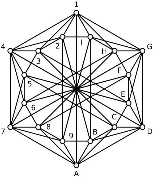
	$v_{1}$	$v_{2}$	$v_{3}$	$v_{4}$	$v_{5}$	$v_{6}$	$v_{7}$	$v_{8}$	$v_{9}$	$v_{A}$	$v_{B}$	$v_{C}$	$v_{D}$	$v_{E}$	$v_{F}$	$v_{G}$	$v_{H}$	$v_{I}$
$\rule{0.0pt}{9.10486pt}v_{i1}$	$1$	$0$	$0$	$0$	$1$	$1$	$\bar{1}$	$1$	$t$	$0$	$t$	$\bar{1}$	$1$	$1$	$t$	$0$	$0$	$0$
$v_{i2}$	$0$	$1$	$0$	$0$	$1$	$\bar{1}$	$1$	$1$	$0$	$t$	$0$	$1$	$1$	$\bar{1}$	$0$	$t$	$t$	$0$
$v_{i3}$	$0$	$0$	$1$	$0$	$0$	$t$	$t$	$0$	$1$	$\bar{1}$	$\bar{1}$	$0$	$t$	$0$	$\bar{1}$	$\bar{1}$	$1$	$1$
$v_{i4}$	$0$	$0$	$0$	$1$	$0$	$0$	$0$	$t$	$\bar{1}$	$\bar{1}$	$1$	$t$	$0$	$t$	$\bar{1}$	$1$	$\bar{1}$	$1$
$w_{i}$	$1$	$1$	$1$	$1$	$1$	$1$	$1$	$1$	$1$	$1$	$1$	$1$	$1$	$1$	$1$	$1$	$1$	$1$

Table 2: CEG-18. Each column $v_{i}$ corresponds to one observable represented by the projector $|v_{i}\rangle\langle v_{i}|$. The labels correspond to those in with Fig. 1. The rows $v_{ij}$ give the components of $|v_{i}\rangle$ (unnormalized). $\bar{1}=-1$ and $t=\sqrt{2}$. The last row contains the weights of the optimal SI-C witness of the form (1). The weights $w_{ij}$ in (1) can be chosen in any way that satisfies $w_{ij}\geq\max\{w_{i},w_{j}\}$. With these weights, $\alpha(G,\vec{w})=4$ and $\theta(G,\vec{w})=\frac{9}{2}$.

Figure 1: Graph of compatibility of CEG-18. Nodes represent observables and edges connect compatible observables. The labels refer to the observables in Table 2.

The last row of Table 2 provides the weights corresponding to the optimal SI-C witness of the form (1).

B.5 Proof that CEG-18 is unique up to unitary transformations

Suppose that you have the $L_{1},\ldots,L_{18}$ with the same relations of orthogonality as the vectors $v_{1},\ldots,v_{9},v_{A},\ldots,v_{I}$ in Table 2 and Fig. 1. Without loss of generality, we can assume that

$$\begin{split}&L_{1}=[\mathds{1}_{d},0,0,0],\;\;\;\;L_{2}=[0,\mathds{1}_{d},0,0],\\ &L_{3}=[0,0,\mathds{1}_{d},0],\;\;\;\;L_{4}=[0,0,0,\mathds{1}_{d}].\end{split}$$ (58)

Hereafter, for simplicity, we will use $\mathds{1}$ rather than $\mathds{1}_{d}$.

Without loss of generality, we can assume that

$$L_{5}=[\mathds{1},A,0,0].$$ (59)

Then, $L_{6}\perp L_{4}$ and $L_{6}\perp L_{5}$ imply

$$L_{6}=[\mathds{1},-(A^{-1})^{\dagger},B,0].$$ (60)

Similarly, $L_{7}\perp L_{4}$ and $L_{7}\perp L_{5}$ imply

$$L_{7}=[\mathds{1},-(A^{-1})^{\dagger},C,0].$$ (61)

Since $L_{7}\perp L_{6}$,

$$C=-[\mathds{1}+(AA^{\dagger})^{-1}](B^{-1})^{\dagger}.$$ (62)

From $L_{18}\perp L_{1}$ and $L_{18}\perp L_{2}$, we can assume

$$L_{18}=[0,0,\mathds{1},D].$$ (63)

Since $L_{17}\perp L_{1}$ and $L_{17}\perp L_{18}$,

$$L_{17}=[0,E,\mathds{1},-(D^{-1})^{\dagger}].$$ (64)

In addition, $L_{16}\perp L_{0}$ and $L_{16}\perp L_{18}$ imply

$$L_{16}=[0,F,\mathds{1},-(D^{-1})^{\dagger}].$$ (65)

Since $L_{17}\perp L_{16}$ and $L_{16}\perp L_{7}$,

$$F=[\mathds{1}+(DD^{\dagger})^{-1}](E^{-1})^{\dagger}=-B^{-1}(A+(A^{-1})^{\dagger}).$$ (66)

Hence

$$DD^{\dagger}=(B^{-1}AA^{\dagger}B)^{-1}.$$ (67)

The relation $L_{17}\perp L_{6}$ implies

$$E=B^{\dagger}A.$$ (68)

In addition, $L_{15}\perp L_{2}$, $L_{15}\perp L_{16}$, and $L_{15}\perp L_{17}$ imply

$$L_{15}=[\mathds{1},0,-(B^{-1})^{\dagger},-(B^{-1})^{\dagger}D],$$ (69)

$L_{8}\perp L_{3}$, $L_{8}\perp L_{6}$, and $L_{8}\perp L_{15}$ imply

$$L_{8}=[\mathds{1},A,0,B(D^{-1})^{\dagger}],$$ (70)

$L_{14}\perp L_{3}$, $L_{14}\perp L_{5}$, and $L_{14}\perp L_{16}$ imply

$$L_{14}=[\mathds{1},-(A^{-1})^{\dagger},0,-(A^{-1})^{\dagger}F^{\dagger}D),$$ (71)

$L_{13}\perp L_{4}$, $L_{13}\perp L_{14}$, and $L_{13}\perp L_{15}$ imply

$$L_{13}=[\mathds{1},A,B,0],$$ (72)

$L_{9}\perp L_{2}$, $L_{9}\perp L_{7}$, and $L_{9}\perp L_{18}$ imply

$$L_{9}=[\mathds{1},0,-(C^{-1})^{\dagger},(D^{-1}C^{-1})^{\dagger}],$$ (73)

$L_{10}\perp L_{1}$, $L_{10}\perp L_{7}$, and $L_{10}\perp L_{8}$ imply

$$L_{10}=[0,\mathds{1},(C^{\dagger}A)^{-1},-A(B^{\dagger})^{-1}D].$$ (74)

Since $L_{9}\perp L_{8}$, we have

$$C=-B(DD^{\dagger})^{-1}=-AA^{\dagger}B.$$ (75)

From $L_{10}\perp L_{9}$ and $L_{10}\perp L_{13}$,

$$C=-(A^{\dagger})^{-2}B,\;\;\;\;A=A^{\dagger}.$$ (76)

Therefore, we obtain that $A$ is hermitian and $A^{4}=\mathds{1}$. Hence, the eigenvalues of $A$ can only be $\pm 1$ and $A$ is automatically unitary. We still have some freedom to choose different $A$, $B$, and $D$ by applying a global unitary. We can choose $A=\mathds{1}$. Eq. (67) implies that $D$ is also unitary, we can also choose it to be $\mathds{1}$.

Then, by $L_{16}\perp L_{13}$, we obtain that $BB^{\dagger}=2\mathds{1}$. Hence, we can similarly set $B=\sqrt{2}\mathds{1}$. Consequently,

$$C=-\sqrt{2}\mathds{1},\;\;\;E=\sqrt{2}\mathds{1},\;\;\;F=-\sqrt{2}\mathds{1}.$$ (77)

$L_{12}\perp L_{3}$, $L_{12}\perp L_{5}$, and $L_{12}\perp L_{14}$ imply

$$L_{12}=[\mathds{1},-\mathds{1},0,-\sqrt{2}\mathds{1}].$$ (78)

$L_{11}\perp L_{10}$, $L_{11}\perp L_{12}$, and $L_{11}\perp L_{13}$ imply

$$L_{11}=[\sqrt{2}\mathds{1},0,-\mathds{1},\mathds{1}].$$ (79)

Therefore, up to a global unitary,

$$\Pi_{i}=\ket{v_{i}}\bra{v_{i}}\otimes\mathds{1},\forall i=1,\ldots,18,$$ (80)

where $|v_{i}\rangle$’s are the columns in Table 2.

	$v_{1}$	$v_{2}$	$v_{3}$	$v_{4}$	$v_{5}$	$v_{6}$	$v_{7}$	$v_{8}$	$v_{9}$	$v_{10}$	$v_{11}$	$v_{12}$	$v_{13}$	$v_{14}$	$v_{15}$	$v_{16}$	$v_{17}$	$v_{18}$	$v_{19}$	$v_{20}$	$v_{21}$	$v_{22}$	$v_{23}$	$v_{24}$
$\rule{0.0pt}{9.10486pt}v_{i1}$	$1$	$0$	$0$	$0$	$1$	$1$	$1$	$1$	$1$	$1$	$1$	$\bar{1}$	$1$	$1$	$0$	$0$	$1$	$1$	$0$	$0$	$1$	$1$	$0$	$0$
$v_{i2}$	$0$	$1$	$0$	$0$	$1$	$1$	$\bar{1}$	$\bar{1}$	$1$	$1$	$\bar{1}$	$1$	$1$	$\bar{1}$	$0$	$0$	$0$	$0$	$1$	$1$	$0$	$0$	$1$	$1$
$v_{i3}$	$0$	$0$	$1$	$0$	$1$	$\bar{1}$	$1$	$\bar{1}$	$1$	$\bar{1}$	$1$	$1$	$0$	$0$	$1$	$1$	$1$	$\bar{1}$	$0$	$0$	$0$	$0$	$1$	$\bar{1}$
$v_{i4}$	$0$	$0$	$0$	$1$	$1$	$\bar{1}$	$\bar{1}$	$1$	$\bar{1}$	$1$	$1$	$1$	$0$	$0$	$1$	$\bar{1}$	$0$	$0$	$1$	$\bar{1}$	$1$	$\bar{1}$	$0$	$0$
$w_{i}$	$1$	$1$	$1$	$1$	$1$	$1$	$1$	$1$	$1$	$1$	$1$	$1$	$1$	$1$	$1$	$1$	$1$	$1$	$1$	$1$	$1$	$1$	$1$	$1$

Table 3: Peres-24. Each column $v_{i}$ corresponds to one observable represented by the projector $|v_{i}\rangle\langle v_{i}|$. The rows $v_{ij}$ give the components of $|v_{i}\rangle$ (unnormalized). $\bar{1}=-1$. The last row contains the weights $w_{i}$ of the optimal SI-C witness of the form (1). The weights $w_{ij}$ in (1) can be chosen in any way that satisfies $w_{ij}\geq\max\{w_{i},w_{j}\}$. With these weights, $\alpha(G,\vec{w})=5$ and $Q(G,\vec{w})=\theta(G,\vec{w})=6$.

B.6 Peres-24 and its SI-C witness

Peres-24 is the set of $24$ rank-one projectors in $d=4$ shown in Table 3. It was introduced in [34]. Unlike BBC-21 and CEG-18, Peres-24 is not critical (in the sense of Zimba and Penrose [47]): some observables can be removed while still having a SI-C set. In turn, Peres-24 is a complete SI-C set.

The last row of Table 3 provides the weights corresponding to the optimal SI-C witness of the form (1). As shown in Table 3, Peres-24 is an egalitarian Lovász-optimum SI-C set.

B.7 Proof that Peres-24 is unique up to unitary transformations

Suppose that you have the projectors $\Pi_{1},\ldots,\Pi_{24}$, and, correspondingly, $L_{1},\ldots,L_{24}$ with the same relations of orthogonality as the vectors $v_{1},\ldots,v_{24}$ in Table 3. Without loss of generality, we can take $L_{1}=[\mathds{1}_{d},0,0,0]$, $L_{2}=[0,\mathds{1}_{d},0,0]$, $L_{3}=[0,0,\mathds{1}_{d},0]$, and $L_{4}=[0,0,0,\mathds{1}_{d}]$, where $\mathds{1}_{d}$ is the identity operator in the Hilbert space of dimension $d$. Hereafter, for simplicity, we will omit the subindex $d$, and simply write $\mathds{1}$.

Let us now consider the projectors $L_{13}$, $L_{14}$, $L_{15}$, and $L_{16}$. Since $L_{13}\perp L_{3}$, $L_{13}\perp L_{4}$, $L_{15}\perp L_{1}$, and $L_{15}\perp L_{2}$, by using Eq. (142), we can assume that

$$L_{13}=[\mathds{1},D,0,0],\;\;\;\;L_{15}=[0,0,\mathds{1},E],$$ (81)

where $D$ and $E$ are invertible matrices. Then, due to Eq. (143), $L_{14}\perp L_{3}$, $L_{14}\perp L_{4}$, and $L_{14}\perp L_{13}$ imply

$$L_{14}=[\mathds{1},-(D^{-1})^{\dagger},0,0].$$ (82)

Similarly, $L_{16}\perp L_{1}$, $L_{16}\perp L_{2}$, and $L_{16}\perp L_{15}$ imply

$$L_{16}=[0,0,\mathds{1},-(E^{-1})^{\dagger}].$$ (83)

Let us now consider the projectors $L_{17}$, $L_{18}$, $L_{19}$, and $L_{20}$. Since $L_{17}\perp L_{2}$, $L_{17}\perp L_{4}$, $L_{19}\perp L_{1}$, and $L_{19}\perp L_{3}$, by applying Eq. (142), we can take

$$L_{17}=[\mathds{1},0,F,0],\;\;\;\;L_{19}=[0,\mathds{1},0,G],$$ (84)

where $F$ and $G$ are invertible matrices. Then, $L_{18}\perp L_{2}$, $L_{18}\perp L_{4}$, and $L_{18}\perp L_{17}$ imply

$$L_{18}=[\mathds{1},0,-(F^{-1})^{\dagger},0].$$ (85)

Similarly, $L_{20}\perp L_{1}$, $L_{20}\perp L_{3}$, and $L_{20}\perp L_{19}$ imply

$$L_{20}=[0,\mathds{1},0,-(G^{-1})^{\dagger}].$$ (86)

Let us now consider the projectors $L_{5}$, $L_{6}$, $L_{7}$, and $L_{8}$. Then, $L_{5}\perp L_{14}$, $L_{5}\perp L_{16}$, and $L_{5}\perp L_{18}$ imply

$$L_{5}=[\mathds{1},D,F,FE].$$ (87)

Similarly, $L_{6}\perp L_{14}$, $L_{6}\perp L_{16}$, and $L_{6}\perp L_{17}$ imply

$$L_{6}=[\mathds{1},D,-(F^{-1})^{\dagger},-(F^{-1})^{\dagger}E].$$ (88)

Also, $L_{7}\perp L_{13}$, $L_{7}\perp L_{15}$, and $L_{7}\perp L_{18}$ imply

$$L_{7}=[\mathds{1},-(D^{-1})^{\dagger},F,-F(E^{-1})^{\dagger}].$$ (89)

Finally, $L_{8}\perp L_{13}$, $L_{8}\perp L_{15}$, and $L_{8}\perp L_{17}$ imply

$$L_{8}=[\mathds{1},-(D^{-1})^{\dagger},-(F^{-1})^{\dagger},(F^{-1})^{\dagger}(E^{-1})^{\dagger}].$$ (90)

From $L_{5}\perp L_{20}$ and $L_{6}\perp L_{19}$,

$$DG=FE,\;\;\;\;F^{\dagger}D=EG^{\dagger}.$$ (91)

Let us now consider the projectors $L_{9}$, $L_{10}$, $L_{11}$, and $L_{12}$. Then, $L_{9}\perp L_{14}$, $L_{9}\perp L_{15}$, and $L_{9}\perp L_{18}$ imply

$$L_{9}=[\mathds{1},D,F,-F(E^{-1})^{\dagger}].$$ (92)

Also, $L_{10}\perp L_{14}$, $L_{10}\perp L_{15}$, and $L_{10}\perp L_{17}$ imply

$$L_{10}=[\mathds{1},D,-(F^{-1})^{\dagger},(F^{-1})^{\dagger}(E^{-1})^{\dagger}].$$ (93)

Similarly, $L_{11}\perp L_{13}$, $L_{11}\perp L_{16}$, and $L_{11}\perp L_{18}$ imply

$$L_{11}=[\mathds{1},-(D^{-1})^{\dagger},F,FE].$$ (94)

Finally, $L_{12}\perp L_{13}$, $L_{12}\perp L_{16}$, and $L_{12}\perp L_{18}$ imply

$$L_{12}=[\mathds{1},-(D^{-1})^{\dagger},-(F^{-1})^{\dagger},-(F^{-1})^{\dagger}E].$$ (95)

From $L_{9}\perp L_{19}$ and $L_{10}\perp L_{20}$,

$$D=F(E^{-1})^{\dagger}G^{\dagger},\;\;\;\;D=(F^{-1})^{\dagger}EG^{-1}.$$ (96)

From Eqs. (91) and (96),

$$DD^{\dagger}=EE^{\dagger}=FF^{\dagger}=GG^{\dagger}=\mathds{1}.$$ (97)

We still have the freedom to apply a unitary on subspaces related to $L_{1}$, $L_{2}$, $L_{3}$, and $L_{4}$. Hence, we can set $D=E=F=\mathds{1}$. Then, we have also $G=\mathds{1}$ because of Eq. (91).

Finally, let us consider the projectors $L_{21}$, $L_{22}$, $L_{23}$, and $L_{24}$. Then, $L_{21}\perp L_{2}$, $L_{21}\perp L_{3}$, and $L_{21}\perp L_{6}$ imply

$$L_{21}=[\mathds{1},0,0,\mathds{1}].$$ (98)

Also $L_{22}\perp L_{2}$, $L_{22}\perp L_{3}$, and $L_{22}\perp L_{5}$ imply

$$L_{22}=[\mathds{1},0,0,-\mathds{1}].$$ (99)

Similarly, $L_{23}\perp L_{1}$, $L_{23}\perp L_{4}$, and $L_{23}\perp L_{6}$ imply

$$L_{23}=[0,\mathds{1},\mathds{1},0].$$ (100)

Finally, $L_{24}\perp L_{1}$, $L_{24}\perp L_{4}$, and $L_{24}\perp L_{5}$ imply

$$L_{24}=[0,\mathds{1},-\mathds{1},0].$$ (101)

Then, it easy to check that all the remaining orthogonality relations in Table 3 are satisfied.

Using that for $i\in V$ and $(j,t)\in\{1,\dots,c\}$ such that $(i,j)\notin E$ and $(i,t)\in E$, each rank-$k$ projector $\Pi_{i}$ that acts on $\mathbbm{C}^{d}$ can be decomposed as

$$\Pi_{i}=L_{i}^{\dagger}(L_{i}L_{i}^{\dagger})^{-1}L_{i},\;\;\;\;L_{i}=[B_{1i},B_{2i},\ldots,B_{ci}],$$ (102)

it is easy to see that Peres-24 can be written in the form $\Pi_{i}=|v_{i}\rangle\langle v_{i}|\otimes\mathds{1}$, where the $|v_{i}\rangle$’s are the columns in Table 3.

B.8 The magic square and its SI-C witness

Given 9 observables, $A$, $B$, $C$, $a$, $b$, $c$, $\alpha$, $\beta$, and $\gamma$, with possible outcomes $-1$ or $1$, the following inequality [5] holds for any NCHV theory:

$$\braket{ABC}+\braket{abc}+\braket{\alpha\beta\gamma}+\braket{Aa\alpha}+\braket{Bb\beta}-\braket{Cc\gamma}\overset{\rm NCHV}{\leqslant}4.$$ (103)

However, if we consider the following two-qubit observables:

$$\begin{bmatrix}A&B&C\\ a&b&c\\ \alpha&\beta&\gamma\end{bmatrix}=\begin{bmatrix}\sigma_{z}\otimes\mathds{1}&\mathds{1}\otimes\sigma_{z}&\sigma_{z}\otimes\sigma_{z}\\ \mathds{1}\otimes\sigma_{x}&\sigma_{x}\otimes\mathds{1}&\sigma_{x}\otimes\sigma_{x}\\ \sigma_{z}\otimes\sigma_{x}&\sigma_{x}\otimes\sigma_{z}&\sigma_{y}\otimes\sigma_{y}\end{bmatrix},$$ (104)

then the left-hand side of (103) is $6$, since, for any two-qubit state,

$$\braket{ABC}=\braket{abc}=\braket{Aa\alpha}=\braket{Bb\beta}=-\braket{Cc\gamma}=1.$$ (105)

The observables in (104) were introduced by Peres and Mermin [11, 12]. The right-hand side of (104) is usually referred to as the Peres-Mermin square or magic square.

The Peres-Mermin square is a SI-C set (although not of rank-one projectors) and inequality (103) is equally violated by any quantum state in $d=4$ [although it is not of the form (1)].

B.9 The relation between the magic square and Peres-24

The Peres-Mermin square is related to Peres-24 [34]. Each row or column in (104) contains compatible observables represented by operators whose product is $\mathds{1}$, except for the last column, which is $-\mathds{1}$. This implies that, according to QM, only four events can happen for every set of three compatible observables. If, e.g., $[-+-|ABC]$ denotes the event: the results $-1$, $1$, and $-1$ are obtained when $A$, $B$, and $C$ are measured, respectively, then only the following $24$ events can happen: $[+++|ABC]$, $[+--|ABC]$, $[-+-|ABC]$, $[--+|ABC]$, $[+++|abc]$, $[+--|abc]$, $[-+-|abc]$, $[--+|abc]$, $[+++|\alpha\beta\gamma]$, $[+--|\alpha\beta\gamma]$, $[-+-|\alpha\beta\gamma]$, $[--+|\alpha\beta\gamma]$, $[+++|Aa\alpha]$, $[+--|Aa\alpha]$, $[-+-|Aa\alpha]$, $[--+|Aa\alpha]$, $[+++|Bb\beta]$, $[+--|Bb\beta]$, $[-+-|Bb\beta]$, $[--+|Bb\beta]$, $[++-|Cc\gamma]$, $[+-+|Cc\gamma]$, $[-++|Cc\gamma]$, and $[---|Cc\gamma]$. Each of these events is represented by a projector, which is the eigenprojector of the corresponding Hermitian operators with the corresponding eigenvalues. The $24$ projectors thus defined have the same orthogonality relations as the $24$ projectors of Peres-24. The relation between the Peres-Mermin square and Peres-24 allows us to prove that the magic square is unique up to unitary transformations.

For any set $\{A,B,C,a,b,c,\alpha,\beta,\gamma\}$ with the same relations of joint measurability given in Eq. (104) and whose products fulfil the same relationships as those fulfilled by the observables in Eq. (104), we can obtain $24$ vectors with the same relations of orthogonality as those of Peres-24. Let us call $\{\Pi_{i}\}_{i=1}^{24}$ this set of rank-one projectors. As seen before, there is a unitary transformation $U$ such that $U(\Pi_{i})U^{\dagger}=|v_{i}\rangle\langle v_{i}|\otimes\mathds{1}:=\tilde{\Pi}_{i}$, where $|v_{i}\rangle$ are the columns in Table 3.

B.10 Proof that the magic square is unique up to unitary transformations

Since $A$, $B$, and $C$ are compatible, then

$$A^{+}B^{+}\succeq A^{+}B^{+}C^{+},$$ (106a)

$$A^{+}B^{-}\succeq A^{+}B^{-}C^{-},$$ (106b)

$$A^{-}B^{+}\succeq A^{-}B^{+}C^{-},$$ (106c)

$$A^{-}B^{-}\succeq A^{-}B^{-}C^{+},$$ (106d)

where $A^{+}$ and $A^{-}$ denote the projectors for the positive and negative eigenspaces of $A$, respectively. That is, $A=A^{+}-A^{-}$. Hence,

$$U(A^{+})U^{\dagger} =U(A^{+}B^{+}+A^{+}B^{-})U^{\dagger}$$

$$\succeq U(A^{+}B^{+}C^{+})U^{\dagger}+U(A^{+}B^{-}C^{-})U^{\dagger}$$

$$=U(\Pi_{1})U^{\dagger}+U(\Pi_{2})U^{\dagger}$$

$$=\tilde{\Pi}_{1}+\tilde{\Pi}_{2},$$ (107)

$$U(A^{-})U^{\dagger} =U(A^{-}B^{+}+A^{-}B^{-})U^{\dagger}$$

$$\succeq U(A^{-}B^{+}C^{-})U^{\dagger}+U(A^{-}B^{-}C^{+})U^{\dagger}$$

$$=U(\Pi_{3})U^{\dagger}+U(\Pi_{4})U^{\dagger}$$

$$=\tilde{\Pi}_{3}+\tilde{\Pi}_{4}.$$ (108)

In addition,

$$A^{+}+A^{-}=\mathds{1}$$ (109)

and

$$\tilde{\Pi}_{1}+\tilde{\Pi}_{2}+\tilde{\Pi}_{3}+\tilde{\Pi}_{4}=\mathds{1},$$ (110)

which implies

$$U(A^{+})U^{\dagger}=\tilde{\Pi}_{1}+\tilde{\Pi}_{2},\;\;\;\;U(A^{-})U^{\dagger}=\tilde{\Pi}_{3}+\tilde{\Pi}_{4}.$$ (111)

Consequently,

$$U(A)=U(A^{+})U^{\dagger}-U(A^{-})U^{\dagger}=\begin{bmatrix}1&&&\\ &1&&\\ &&\bar{1}&\\ &&&\bar{1}\end{bmatrix}\otimes\mathds{1}_{k},$$ (112)

where $k=D/4$. Similarly, other observables in the realization can be mapped with the same unitary $U$ into the ones in Eq. (104).

	$v_{1}$	$v_{2}$	$v_{3}$	$v_{4}$	$v_{5}$	$v_{6}$	$v_{7}$	$v_{8}$	$v_{9}$	$v_{10}$	$v_{11}$	$v_{12}$	$v_{13}$	$v_{14}$	$v_{15}$	$v_{16}$	$v_{17}$	$v_{18}$	$v_{19}$	$v_{20}$	$v_{21}$	$v_{22}$	$v_{23}$	$v_{24}$	$v_{25}$	$v_{26}$	$v_{27}$	$v_{28}$	$v_{29}$	$v_{30}$	$v_{31}$	$v_{32}$	$v_{33}$	$v_{34}$	$v_{35}$	$v_{36}$	$v_{37}$	$v_{38}$	$v_{39}$
$\rule{0.0pt}{9.10486pt}v_{i1}$	$1$	$0$	$0$	$0$	$1$	$1$	$1$	$1$	$1$	$1$	$1$	$1$	$1$	$1$	$0$	$0$	$1$	$1$	$0$	$0$	$1$	$1$	$0$	$0$	$0$	$0$	$0$	$0$	$0$	$0$	$0$	$0$	$0$	$0$	$0$	$0$	$0$	$0$	$0$
$v_{i2}$	$0$	$1$	$0$	$0$	$1$	$1$	$\bar{1}$	$\bar{1}$	$1$	$1$	$\bar{1}$	$\bar{1}$	$1$	$\bar{1}$	$0$	$0$	$0$	$0$	$1$	$1$	$0$	$0$	$1$	$1$	$0$	$1$	$1$	$1$	$1$	$1$	$1$	$1$	$1$	$0$	$0$	$0$	$0$	$1$	$1$
$v_{i3}$	$0$	$0$	$1$	$0$	$1$	$\bar{1}$	$1$	$\bar{1}$	$1$	$\bar{1}$	$1$	$\bar{1}$	$0$	$0$	$1$	$1$	$1$	$\bar{1}$	$0$	$0$	$0$	$0$	$1$	$\bar{1}$	$0$	$1$	$1$	$\bar{1}$	$\bar{1}$	$1$	$1$	$\bar{1}$	$\bar{1}$	$0$	$0$	$1$	$1$	$0$	$0$
$v_{i4}$	$0$	$0$	$0$	$1$	$1$	$\bar{1}$	$\bar{1}$	$1$	$\bar{1}$	$1$	$1$	$\bar{1}$	$0$	$0$	$1$	$\bar{1}$	$0$	$0$	$1$	$\bar{1}$	$1$	$\bar{1}$	$0$	$0$	$0$	$1$	$\bar{1}$	$1$	$\bar{1}$	$1$	$\bar{1}$	$1$	$\bar{1}$	$1$	$1$	$0$	$0$	$0$	$0$
$v_{i5}$	$0$	$0$	$0$	$0$	$0$	$0$	$0$	$0$	$0$	$0$	$0$	$0$	$0$	$0$	$0$	$0$	$0$	$0$	$0$	$0$	$0$	$0$	$0$	$0$	$1$	$1$	$\bar{1}$	$\bar{1}$	$1$	$\bar{1}$	$1$	$1$	$\bar{1}$	$1$	$\bar{1}$	$1$	$\bar{1}$	$1$	$\bar{1}$
$w_{i}$	$24$	$8$	$8$	$8$	$4$	$4$	$4$	$4$	$4$	$4$	$4$	$4$	$6$	$6$	$7$	$7$	$6$	$6$	$7$	$7$	$6$	$6$	$7$	$7$	$24$	$4$	$4$	$4$	$4$	$4$	$4$	$4$	$4$	$6$	$6$	$6$	$6$	$6$	$6$

Table 4: Peres-39. Each column $v_{i}$ corresponds to one observable represented by the projector $|v_{i}\rangle\langle v_{i}|$. The rows $v_{ij}$ give the components of $|v_{i}\rangle$ (unnormalized). $\bar{1}=-1$. The last row contains the weights $w_{i}$ of the optimal SI-C witness of the form (116). With these weights, $\alpha(G,\vec{w})=46$ and $Q(G,\vec{w})=\vartheta(G,\vec{w})=50$.

B.11 Peres-39 and its witness

One can obtain a KS set in $d=5$ by taking the $4$-dimensional vectors of Peres-24 and either appending or prepending $0$ to them [35]. That is, if we call $\{\ket{u_{i}}\}_{i=1}^{24}$ the set of vectors in Peres-24, then

$$\mathcal{V}=\{\ket{\mu_{i}}\}_{i=1}^{24}\cup\{\ket{\nu_{i}}\}_{i=1}^{24},$$ (113)

where

$$\bra{\mu_{i}}=(\bra{u_{i}},0),\;\;\;\;\bra{\nu_{i}}=(0,\bra{u_{i}}).$$ (114)

is a KS set in $d=5$. $\mathcal{V}$ only contains $39$ vectors, since

$$\ket{\mu_{2}} =\ket{\nu_{1}},\;\; \ket{\mu_{3}} =\ket{\nu_{2}},\;\; \ket{\mu_{4}} =\ket{\nu_{3}},$$

$$\ket{\mu_{15}} =\ket{\nu_{23}},\;\; \ket{\mu_{16}} =\ket{\nu_{24}},\;\; \ket{\mu_{19}} =\ket{\nu_{17}},$$

$$\ket{\mu_{20}} =\ket{\nu_{18}},\;\; \ket{\mu_{23}} =\ket{\nu_{13}},\;\; \ket{\mu_{24}} =\ket{\nu_{14}}.$$ (115)

The resulting set is shown in Table 4. Hereafter, we will call it Peres-39.

Let us consider the following witness:

$${\cal W}^{\prime}:=\sum_{C\in{\cal C}_{5}}\sum_{i\in C}P(\Pi_{i}=1)=\sum_{i=1}^{39}w_{i}P(\Pi_{i}=1)\leq\alpha(G_{39},w),$$ (116)

where $G_{39}$ is the graph of compatibility of Peres-39, ${\cal C}_{5}$ is the set of cliques of size $5$ in $G_{39}$, and $w_{i}$ is the frequency of $i$ in ${\cal C}$, which is shown in Table 4. Strictly speaking, ${\cal W}^{\prime}$ is not a SI-C witness like those in Eq. (1) in which every $\Pi_{i}$ is in several contexts. Probably, there is a proper SI-C witness of the form (1) for Peres-39, but we have not computational power to obtain it. Instead, we will assume that the projectors $\{\Pi_{i}\}$ in (116) provides a quantum realization of the graph of orthogonality corresponding to $G_{39}$. Under this assumption, inequality (116) holds.

For any state of $d=5$, $Q(G_{39},w)=\vartheta(G_{39},w)=|{\cal C}|$, which is the number of elements in ${\cal C}$ and therefore is also the algebraic maximum of ${\cal W}^{\prime}$. This shows that Peres-39 is an egalitarian Lovász-optimum SI-C set.

B.12 Proof that Peres-39 is unique up to unitary transformations

By construction, in Peres-39, $\{\ket{\mu}_{i}\}_{i=1}^{24}$ contains only vectors orthogonal to $(0,0,0,0,1)$. Hence, all the basis of size $5$ which contains $(0,0,0,0,1)$ are just all the basis of size $4$ which are all orthogonal to $(0,0,0,0,1)$, i.e., all the complete basis in the subspace spanned by $\{\ket{\mu}_{i}\}_{i=1}^{24}$.

Let us write Peres-39 as $\{P_{i}\}_{i=1}^{24}\cup\{Q_{i}\}_{i=1}^{24}$, where $P_{i}=Q_{j}$ if $\ket{\mu_{i}}=\ket{\nu_{j}}$. Then, $\{P_{i}\}_{i=1}^{24}$ is a realization of Peres-24 in the $4$-dimensional subspace spanned by $\{P_{i}\}_{i=1}^{24}$. Similarly, $\{Q_{i}\}_{i=1}^{24}$ is a realization of Peres-24 in the subspace spanned by $\{Q_{i}\}_{i=1}^{24}$. Then, we can apply that Peres-24 allows for FRC to each of them in their corresponding subspaces. Since the intersection of $\{P_{i}\}_{i=1}^{24},\{Q_{i}\}_{i=1}^{24}$ is not empty, all the projectors in the realization of Peres-39 have the same rank.

Without loss of generality, we can assume that

$$P_{i}=|\mu_{i}\rangle\langle\mu_{i}|\otimes\mathds{1}_{d/5},\;\;\forall i=1,\ldots,24.$$ (117)

In addition, $Q_{4}=|\nu_{4}\rangle\langle\nu_{4}|\otimes\mathds{1}_{d/5}$. Then, we can copy for $\{Q_{i}\}_{i=1}^{24}$ the proof we used for Peres-24. Since $Q_{i}$ is fixed already for $i=1,2,3,13,14,17,18,23,24$, we know that $D=F=\mathds{1}$ as in Eqs. (81) and (84) and, consequently, that

$$E=G,\;\;\;\;EG^{\dagger}=\mathds{1}.$$ (118)

Note that we still have the freedom to apply a local unitary to the subspace represented by $Q_{4}$. This implies that we can set $E=G=\mathds{1}$, which fix the whole realization up to unitary transformations. Direct computation shows $\{P_{i}\}_{i=1}^{24}\cup\{Q_{i}\}_{i=1}^{24}$ realizes all the orthogonality relations in $G_{39}$.

B.13 Proof that all the KS sets in $d\geq 6$ are unique up to unitary transformations

For any dimension $d\geqslant 4$, by patching $d-3$ copies of Peres-24 together (as we did in the construction leading to Peres-39), we can obtain a SI-C set in dimension $d$, which allows for FRC with respect to the witness (116) and the orthogonality relations encoded in this set.

We can prove this recursively. Let us assume that we can prove it for the $d$-dimensional case. In the $(d+1)$-dimensional SI-C set, all the vectors whose last element is $0$ constitute, by construction, a $d$-dimensional SI-C set. We denote it as $\mathcal{P}$. In addition, we denote $\mathcal{Q}$ the last added Peres-24 SI-C set. Hence, all the maximal cliques of size $d+1$ which contain $(0,\ldots,0,1)$ correspond to all the maximal cliques of size $d$ for the $d$-dimensional SI-C set $\mathcal{P}$. As we discussed in the FRC of Peres-39, the fact that all the maximal cliques of size $d+1$ are complete bases leads to the fact that all the maximal cliques of size $d$ in $\mathcal{P}$ are complete bases for the subspace spanned by $\mathcal{P}$. Consequently, $\mathcal{P}$ allows for FRC.

By construction, the set of the vectors living in the last $5$ dimensions is a Peres-39, whose intersection with $\mathcal{P}$ is a Peres-24 $\mathcal{P}^{\prime}$. After the FRC of $\mathcal{P}$, the Peres-24 $\mathcal{P}^{\prime}$ is fixed. Same as in the FRC of Peres-39, this fixes the last added Peres-24 $\mathcal{Q}$ up to unitary transformations. Summing up, we have shown that the $(d+1)$-dimensional SI-C set allows for FRC.

	$v_{1}$	$v_{2}$	$v_{3}$	$v_{4}$	$v_{5}$	$v_{6}$	$v_{7}$	$v_{8}$	$v_{9}$	$v_{A}$	$v_{B}$	$v_{C}$	$v_{D}$
$\rule{0.0pt}{9.10486pt}v_{i1}$	$1$	$0$	$0$	$0$	$0$	$1$	$1$	$1$	$1$	$1$	$1$	$\bar{1}$	$1$
$v_{i2}$	$0$	$1$	$0$	$1$	$1$	$0$	$0$	$1$	$\bar{1}$	$1$	$1$	$1$	$\bar{1}$
$v_{i3}$	$0$	$0$	$1$	$1$	$\bar{1}$	$1$	$\bar{1}$	$0$	$0$	$1$	$\bar{1}$	$1$	$1$
$w_{i}$	$3$	$3$	$3$	$3$	$3$	$3$	$3$	$3$	$3$	$2$	$2$	$2$	$2$

Table 5: YO-13. Each column $v_{i}$ corresponds to one observable represented by the projector $|v_{i}\rangle\langle v_{i}|$. The rows $v_{ij}$ give the components of $|v_{i}\rangle$ (unnormalized). $\bar{1}=-1$. The last row contains the weights $w_{i}$ of the optimal SI-C witness of the form (1). The weights $w_{ij}$ in (1) can be chosen in any way that satisfies $w_{ij}\geq\max\{w_{i},w_{j}\}$. With these weights, $\alpha(G,\vec{w})=11$ and, for any qutrit state, $Q(G,\vec{w})=\frac{35}{3}\approx 11.67$. However, $\vartheta(G,\vec{w})\approx 11.977641$.

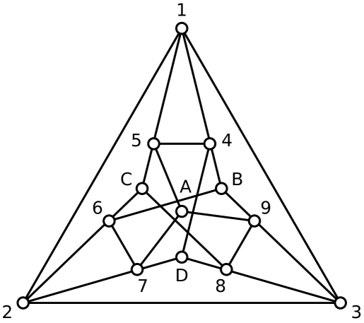
Figure 2: Graph of compatibility of YO-13. Nodes represent observables and edges connect compatible observables. The nodes are labeled as the subindexes in Table 5.

B.14 YO-13

YO-13 is the set of 13 rank-one projectors in $d=3$ shown in Table 5 and whose graph of compatibility is shown in Fig. 2. YO-13 was introduced in [7]. As shown in Table 5, YO-13 is an egalitarian SI-C set with respect to a contextuality witness of the form (1) and YO-13 is not Lovász-optimum. As proven in [36], YO-13 is the smallest SI-C set of rank-one projectors in QM (in any dimension). As it can be easily checked, YO-13 is not a KS set.

B.15 Proof that YO-13, with normalization constraints, is unique up to unitary transformations

YO-13 is unique up to unitary transformations if we assume the following normalization constraints:

$$p_{1}+p_{2}+p_{3}=1,$$

$$p_{1}+p_{4}+p_{5}=1,$$

$$p_{2}+p_{6}+p_{7}=1,$$

$$p_{3}+p_{8}+p_{9}=1,$$ (119)

where $p_{i}$ is the probability of obtaining the outcome $1$ when the projector $|v_{i}\rangle\langle v_{i}|$ is measured, with $v_{i}$ defined in Table. 5.

Following the same notation as before, without loss of generality, we can assume that

$$L_{1}=[\mathds{1}_{d},0,0],\;\;\;L_{2}=[0,\mathds{1}_{d},0],\;\;\;L_{3}=[0,0,\mathds{1}_{d}].$$ (120)

Hereafter, for simplicity, we will omit the subindex $d$. Since $L_{1}\perp L_{4}$ and $L_{1}\perp L_{5}$, we can assume that

$$L_{4}=[0,\mathds{1},A],\;\;\;\;L_{5}=[0,\mathds{1},A^{\prime}].$$ (121)

Then, since $L_{4}\perp L_{5}$,

$$A^{\prime}=-(A^{-1})^{\dagger}.$$ (122)

Similarly,

$$L_{6}=[\mathds{1},0,B],\;\;\;\;L_{7}=[\mathds{1},0,-(B^{-1})^{\dagger}],$$ (123)

$$L_{8}=[\mathds{1},C,0],\;\;\;\;L_{9}=[\mathds{1},-(C^{-1})^{\dagger},0].$$ (124)

Let us assume that

$$L_{A}=[\mathds{1},D,E],\;\;\;\;L_{B}=[\mathds{1},F,G],$$ (125)

$$L_{C}=[\mathds{1},H,I],\;\;\;\;L_{D}=[\mathds{1},J,K].$$ (126)

Then, $L_{A}\perp L_{7}$ and $L_{A}\perp L_{9}$ imply

$$D=C,\;\;\;\;E=B,$$ (127)

$L_{B}\perp L_{6}$ and $L_{B}\perp L_{9}$ imply

$$F=C,\;\;\;\;G=-(B^{-1})^{\dagger},$$ (128)

$L_{C}\perp L_{6}$ and $L_{C}\perp L_{8}$ imply

$$H=-(C^{-1})^{\dagger},\;\;\;\;I=-(B^{-1})^{\dagger},$$ (129)

$L_{D}\perp L_{7}$ and $L_{D}\perp L_{8}$ imply

$$J=-(C^{-1})^{\dagger},\;\;\;\;K=B.$$ (130)

In addition, $L_{5}\perp L_{A}$ and $L_{5}\perp L_{C}$ imply

$$D=-E(A^{\prime})^{\dagger},\;\;\;\;H=-I(A^{\prime})^{\dagger}.$$ (131)

This implies that,

$$B=CA,\;\;\;\;C=BA^{\dagger}.$$ (132)

Then, $L_{4}\perp L_{B}$ and $L_{4}\perp L_{D}$ imply

$$F=-GA^{\dagger},\;\;\;\;J=-KA^{\dagger}.$$ (133)

This implies that,

$$C^{-1}=AB^{\dagger},\;\;\;\;C^{\dagger}=AB^{-1}.$$ (134)

Hence,

$$AA^{\dagger}=BB^{\dagger}=\mathds{1}.$$ (135)

Since we still have the freedom to rotate the subspaces corresponding to $L_{2}$ and $L_{3}$, we can set $A=B=\mathds{1}$. Therefore,

$$C=D=E=F=K=\mathds{1},\;\;\;\;G=H=I=J=-\mathds{1}.$$ (136)

This implies that there is an isometry between $\{\Pi_{i}\}_{i}$ and ${2\ket{v_{i}}\bra{v_{i}}-\mathds{1}_{3}}_{i}$, where $\{v_{i}\}_{i3}$ are the vectors in Table. 5.

	$v_{1}$	$v_{2}$	$v_{3}$	$v_{4}$	$v_{5}$	$v_{6}$	$v_{7}$	$v_{8}$	$v_{9}$	$v_{10}$	$v_{11}$	$v_{12}$	$v_{13}$	$v_{14}$	$v_{15}$	$v_{16}$	$v_{17}$	$v_{18}$	$v_{19}$	$v_{20}$	$v_{21}$	$v_{22}$	$v_{23}$	$v_{24}$	$v_{25}$	$v_{26}$	$v_{27}$	$v_{28}$	$v_{29}$	$v_{30}$	$v_{31}$	$v_{32}$	$v_{33}$
$\rule{0.0pt}{9.10486pt}v_{i1}$	$1$	$0$	$0$	$0$	$0$	$1$	$1$	$1$	$1$	$0$	$0$	$\bar{1}$	$1$	$\bar{1}$	$1$	$0$	$0$	$t$	$t$	$t$	$t$	$\bar{1}$	$\bar{1}$	$1$	$1$	$\bar{1}$	$\bar{1}$	$1$	$1$	$t$	$t$	$t$	$t$
$v_{i2}$	$0$	$1$	$0$	$1$	$1$	$\bar{1}$	$1$	$0$	$0$	$\bar{1}$	$1$	$0$	$0$	$t$	$t$	$t$	$t$	$0$	$0$	$\bar{1}$	$1$	$\bar{1}$	$1$	$\bar{1}$	$1$	$t$	$t$	$t$	$t$	$\bar{1}$	$\bar{1}$	$1$	$1$
$v_{i3}$	$0$	$0$	$1$	$\bar{1}$	$1$	$0$	$0$	$\bar{1}$	$1$	$t$	$t$	$t$	$t$	$0$	$0$	$\bar{1}$	$1$	$\bar{1}$	$1$	$0$	$0$	$t$	$t$	$t$	$t$	$\bar{1}$	$1$	$\bar{1}$	$1$	$\bar{1}$	$1$	$\bar{1}$	$1$
$w_{i}$	$3$	$3$	$3$	$1$	$1$	$1$	$1$	$1$	$1$	$1$	$1$	$1$	$1$	$1$	$1$	$1$	$1$	$1$	$1$	$1$	$1$	$1$	$1$	$1$	$1$	$1$	$1$	$1$	$1$	$1$	$1$	$1$	$1$

Table 6: Peres-33. Each column $v_{i}$ corresponds to one observable represented by the projector $|v_{i}\rangle\langle v_{i}|$. The rows $v_{ij}$ give the components of $|v_{i}\rangle$ (unnormalized). $\bar{1}=-1$ and $t=\sqrt{2}$. The last row contains the weights $w_{i}$ of the optimal SI-C witness of the form (1), where the weights $w_{ij}$ in (1) can be chosen in any way that satisfies $w_{ij}\geq\max\{w_{i},w_{j}\}$. With these weights, $\alpha(G,\vec{w})=12$ and $Q(G,\vec{w})=\vartheta(G,\vec{w})=13$ for all qutrit states.

B.16 Peres-33 and its optimum contextuality witness

Peres-33 is the KS set of rank-one projectors in $d=3$ shown in Table 6. It was introduced in [34]. It is the KS set in $d=3$ with the smallest number of bases known ($16$).

B.17 Proof that Peres-33 is not unique up to unitary transformations

The existence of unitarily inequivalent orthogonality representations of the orthogonality graph of Peres-33 has already been proven in Refs. [48, 49]. For completeness, we provide another proof here.

As shown below, Peres-33 contains, induced, three copies of YO-13. Specifically, using the notation of Table 6, the three copies are

$$S_{1} =\{v_{1},v_{4},v_{5},v_{2},v_{3},v_{30},v_{33},v_{31},v_{32},v_{14},v_{13},v_{15},v_{12}\},$$ (137a)

$$S_{2} =\{v_{2},v_{8},v_{9},v_{1},v_{3},v_{26},v_{29},v_{27},v_{28},v_{20},v_{11},v_{21},v_{10}\},$$ (137b)

$$S_{3} =\{v_{3},v_{6},v_{7},v_{1},v_{2},v_{22},v_{25},v_{23},v_{24},v_{18},v_{17},v_{19},v_{16}\}.$$ (137c)

The graph of compatibility of each copy $S_{k}$ corresponds to the graph in Fig. 2, assuming that the ordering of the vectors in Eqs. (137) is the same used in Table 5. Notice that $S_{i}\cap S_{j}=(1,2,3):=S_{0}$ for $i\neq j$, but otherwise, the three sets are not tightly connected to each other.

A direct calculation shows that there is another realization of the graph of compatibility of Peres-33, where

$$\langle u_{i}|=\begin{cases}(v_{i1},v_{i2},v_{i3}),i\in S_{1}\\ (v_{i1},v_{i2},\mathbbm{i}v_{i3}),i\in S^{\prime}_{2}\\ (v_{i1},-\mathbbm{i}v_{i2},v_{i3}),i\in S^{\prime}_{3},\end{cases}$$ (138)

where $v_{ij}$ are the ones in Table 6 and $S^{\prime}_{2}=S_{2}\setminus S_{0}$, $S^{\prime}_{3}=S_{3}\setminus S_{0}$. However, $\{|v_{i}\rangle\}_{i=1}^{33}$ and $\{|u_{i}\rangle\}_{i=1}^{33}$ cannot be transformed to each other by either a unitary or an antiunitary transformation, since the set $\{|\langle u_{i}|u_{j}\rangle|\}$ is different from $\{|\langle v_{i}|v_{j}\rangle|\}$.

Appendix C Tools used in the proof of Result 2

Consider the situation in which we are given a set of black boxes, each of them supposedly implementing an ideal measurement of one of the elements of a SI-C set $\{\Pi_{i}\}$ with graph of compatibility $G$ (with vertex set $V$ and edge set $E$) and whose optimal noncontextuality inequality of the form (1) has weights $\{w_{i}\}$ given in the proof of Result 1.

Firstly, we consider the case with perfect orthogonality relations and the imperfectness is only in the violation.

Lemma 4.

If, for any quantum state,

$$P(\Pi_{i}=\Pi_{j}=1)=0$$ (139)

for any $(i,j)\in E$ and

$$\sum_{i\in V}w_{i}P(\Pi_{i}=1)>Q-\epsilon,$$ (140)

where $Q$ is $\frac{35}{3}$, $\frac{9}{2}$, $6$, and $10$, and $\epsilon$ is $0.13159$, $0.13397$, $0.17712$, and $0.20808$ for, respectively, BBC-21, CEG-18, Peres-24, and YO-13, and, only in the case of YO-13, for any quantum state satisfying

$$P(\Pi_{1}=1)+P(\Pi_{2}=1)+P(\Pi_{3}=1) =1,$$ (141a)

$$P(\Pi_{1}=1)+P(\Pi_{4}=1)+P(\Pi_{5}=1) =1,$$ (141b)

$$P(\Pi_{2}=1)+P(\Pi_{6}=1)+P(\Pi_{7}=1) =1,$$ (141c)

$$P(\Pi_{3}=1)+P(\Pi_{8}=1)+P(\Pi_{9}=1) =1,$$ (141d)

then,

• $\forall(i,j)\notin E$, $\mathrm{rank}(\Pi_{j}\Pi_{i}\Pi_{j})=\mathrm{rank}(\Pi_{j})$.

• $\forall i\in V$, rank of $\Pi_{i}$ is the same, say, $\mathrm{rank}(\Pi_{i})=k$.

• For $i\in V$ and $(j,t)\in\{1,\dots,c\}$ such that $(i,j)\notin E$ and $(i,t)\in E$, each rank-$k$ projector $\Pi_{i}$ that acts on $\mathbbm{C}^{d}$ can be decomposed as

  $$\Pi_{i}=L_{i}^{\dagger}(L_{i}L_{i}^{\dagger})^{-1}L_{i},\;\;\;\;L_{i}=[B_{1i},B_{2i},\ldots,B_{ci}],$$ (142)

  where $L_{i}$ are $d\times k$ matrices, $B_{ji}$ are $k\times k$ invertible matrices, $B_{ti}=\mathbb{O}$ and we can take $B_{ji}=\mathds{1}$ for any $j$. Moreover,

  $$\Pi_{i}\Pi_{t}=\mathbb{O}\implies L_{i}(L_{t})^{\dagger}=\mathbb{O}.$$ (143)

Proof.

The proof of (I) follows from SDP. Notice that $\Pi_{j}\Pi_{i}\Pi_{j}\preceq\Pi_{j}$. If there is a pair $(i,j)\not\in E$ such that $\mathrm{rank}(\Pi_{j}\Pi_{i}\Pi_{j})<\mathrm{rank}(\Pi_{j})$, then there is a unit vector $\ket{v}$ in the subspace represented by $\Pi_{j}$ that is orthogonal to the subspace spanned by the image of $\Pi_{j}\Pi_{i}\Pi_{j}$. This leads to the linear conditions

$$\bra{v}\Pi_{j}\ket{v}=1,\;\bra{v}\Pi_{j}\Pi_{i}\Pi_{j}\ket{v}=\bra{v}\Pi_{i}\ket{v}=0.$$ (144)

That is,

$$T_{jj}=1,\;\;\;\;T_{ii}=0,$$ (145)

where $T_{lk}=\bra{v}\Pi_{l}\Pi_{k}\ket{v}$. By definition, $T_{lk}$ is positive semidefinite. In addition, the orthogonal relations imply that

$$T_{kl}=0,\;\forall(k,l)\in E.$$ (146)

The quantum violation of state $\ket{v}$ is a linear function of $T_{kk}$ whose upper bound can be calculated through the SDP under the conditions $\Pi_{i}\Pi_{j}=0$ for any $(i,j)\in E$ and (144). It cannot always be smaller than $Q-\epsilon$ for all $(i,j)\not\in E$. Hence, if, for any quantum state, the violation is not smaller than $Q-\epsilon$, then $\mathrm{rank}(\Pi_{j}\Pi_{i}\Pi_{j})=\mathrm{rank}(\Pi_{j})$ for any $(i,j)\not\in E$.

Proof of (II). From (I), $\forall(i,j)\not\in E$,

$$\mathrm{rank}(\Pi_{i})\geq\mathrm{rank}(\Pi_{j}\Pi_{i}\Pi_{j})=\mathrm{rank}(\Pi_{j}),$$ (147)

which implies that $\mathrm{rank}(\Pi_{i})=\mathrm{rank}(\Pi_{j})$ for any $(i,j)\not\in E$. Since the complement of $G$ is connected, we conclude that the rank of all the projectors are same.

Proof of (III). Due to (I) and the existence of complete basis with $c$ projectors, we have the relation $d=ck$. Then, each rank-$k$ projector $\Pi_{i}$ can be decomposed as

$$\Pi_{i}=(L^{\prime}_{i})^{\dagger}L^{\prime}_{i},\;\;\;\;L^{\prime}_{i}=[B_{1i},B_{2i},\ldots,B_{ci}],$$ (148)

where $L^{\prime}_{i}$ are some $d\times k$ matrices and $B_{ji}$’s are some $k\times k$ matrices. In the scenarios we considered, we can always choose $\{\Pi_{j}\}_{j=1}^{c}$ to be the complete basis and take it to be the standard basis, that is,

$$L^{\prime}_{1}=[\mathds{1}_{k},0,\ldots,0],$$ (149a)

$$L^{\prime}_{2}=[0,\mathds{1}_{k},\ldots,0],$$ (149b)

$$\vdots$$

$$L^{\prime}_{c}=[0,0,\ldots,\mathds{1}_{k}].$$ (149c)

Using the above decomposition, we have

$$\Pi_{j}\Pi_{i}\Pi_{j}=B_{ji}^{\dagger}B_{ji}.$$ (150)

Due to (I) and Eq. (150), for $(i,j)\not\in E$, $j\in\{1,\ldots,c\}$, the rank of $B_{ji}$ should be $k$ and hence, this matrix $B_{ji}$ is invertible. While for $(i,t)\in E$ and $t\in\{1,\ldots,c\}$ the left-hand-side of Eq. (150) is zero and therefore $B_{ti}=\mathbb{O}$.
Using that $B_{ji}$’s are either invertible or zero-matrices, a straight-forward calculation shows that

$$\forall i,\ \Pi_{i}^{2}=\Pi_{i}\implies L^{\prime}_{i}(L^{\prime}_{i})^{\dagger}=\mathds{1}_{k}$$ (151)

and

$$\Pi_{i}\Pi_{t}=\mathbb{O}\implies L^{\prime}_{i}(L^{\prime}_{t})^{\dagger}=\mathbb{O}.$$ (152)

By taking $L_{i}=B_{ji}^{-1}L^{\prime}_{i}$ for some invertible $B_{ji}$ and by using Eq. (151), we can express $\Pi_{i}$ as

$$\Pi_{i} = (L^{\prime}_{i})^{\dagger}(L^{\prime}_{i}(L^{\prime}_{i})^{\dagger})^{-1}L^{\prime}_{i}$$ (153)

$$= L_{i}^{\dagger}(L_{i}L_{i}^{\dagger})^{-1}L_{i}.$$

Finally, notice that Eq. (152) implies $L_{i}L_{t}^{\dagger}=\mathbb{O}$. ∎

C.1 Robustness with imperfect orthogonality relations

To analyze the robustness when the orthogonality relations have not been exactly ensured, we introduce the following lemmas and one assumption.

Lemma 5.

For a given matrix $T\preceq\lambda_{1}\mathds{1}$ in $\mathcal{H}$, if $\braket{s}{T}{s}=\lambda_{1}$, $\forall\ket{s}\in S$, where $S$ is a linear basis of $\mathcal{H}$, we have $T=\lambda_{1}\mathds{1}$ in $\mathcal{H}$.

Proof.

Obviously, $\lambda_{1}$ should be the maximal eigenvalue of $T$. Consequently, $\braket{s}{T}{s}=\lambda_{1}$ implies that $\ket{s}\in E_{\lambda_{1}}$, where $E_{\lambda_{1}}$ is the eigenspace of $T$ for the eigenvalue $\lambda_{1}$. Hence, by assumption, $S\subseteq E_{\lambda_{1}}$. By definition, $\mathcal{H}=\operatorname{span}(S)$, which implies

$$\mathcal{H}\subseteq E_{\lambda_{1}}.$$ (154)

Thus, $E_{\lambda_{1}}=\mathcal{H}$. Equivalently, $T=\lambda_{1}\mathds{1}$. ∎

Lemma 6.

For any two projectors $\Pi_{1},\Pi_{2}$ from a given setting, if $\mathrm{rank}(\Pi_{1})>\mathrm{rank}(\Pi_{2})$, then $\exists\ket{s}\in\mathcal{S}$ s.t.

$$\braket{s}{\Pi_{1}}{s}=1,\;\;\;\;\braket{s}{\Pi_{2}}{s}=0.$$ (155)

Proof.

The condition $\mathrm{rank}(\Pi_{1})>\mathrm{rank}(\Pi_{2})$ implies that the intersection $S_{0}$ of the subspace s represented by $\Pi_{1}$ and $\mathds{1}-\Pi_{2}$ is not empty, denote $\Pi_{0}$ the projector onto subspace $S_{0}$. Von Neumann has proven that [50]

$$\Pi_{0}=\lim_{n\to\infty}[\Pi_{1}(\mathds{1}-\Pi_{2})]^{n},$$ (156)

where $\Pi_{i},i=0,1,2$ represent the actions of projection instead of matrices.

By definition, there should be at least one state $\ket{s_{0}}\in\mathcal{S}$ such that $\Pi_{0}\ket{s_{0}}\neq 0$, since $\Pi_{0}\neq 0$. Thus, by repeating the projection $\Pi_{1},\Pi_{2}$ with the initial state $\ket{s_{0}}$, we can finally obtain a state $\ket{s}$ such that $\braket{s}{\Pi_{0}}{s}=1$. By definition of $\Pi_{0}$, we know that $\Pi_{1}\succeq\Pi_{0},\Pi_{2}\succeq\Pi_{0}$. Hence, we have

$$\braket{s}{\Pi_{1}}{s}=\braket{s}{\mathds{1}-\Pi_{2}}{s}=1.$$ (157)

∎

Lemma 7.

For any two projectors $\Pi_{1}$ and $\Pi_{2}$ from a given setting, $\forall\epsilon>0$, $\exists\ket{s}\in\mathcal{S}$ such that

$$\braket{s}{\Pi_{1}\Pi_{2}\Pi_{1}}{s}\geq\lambda_{1}(\Pi_{1}\Pi_{2}\Pi_{1})-\epsilon,$$ (158)

where $\lambda_{1}(\cdot)$ is the maximal eigenvalue.

Proof.

If $\Pi_{1}\perp\Pi_{2}$, any choice of $\ket{s}$ gives the conclusion. Otherwise, $\lambda_{1}(\Pi_{1}\Pi_{2}\Pi_{1})>0$. In addition, there is a state $\ket{s}$ such that $\Pi_{1}\Pi_{2}\Pi_{1}\ket{s}\neq 0$. Denote by $\ket{s_{n}}$ the post-measurement state after the repetition, $n$times, of measurements $\Pi_{2}$ and $\Pi_{1}$, that is,

$$\ket{s_{n}}\propto(\Pi_{1}\Pi_{2}\Pi_{1})^{n}\ket{s}.$$ (159)

Since $\lim_{n\to\infty}(\lambda/\lambda_{1})^{n}=0$, for any eigenvalue $\lambda$ of $\Pi_{1}\Pi_{2}\Pi_{1}$ which is less than $\lambda_{1}$, we that

$$\left[\frac{\Pi_{1}\Pi_{2}\Pi_{1}}{\lambda_{1}(\Pi_{1}\Pi_{2}\Pi_{1})}\right]^{n}\to\Pi_{0},n\to\infty,$$ (160)

where $\Pi_{0}$ is the projector of the eigenspace of $\Pi_{1}\Pi_{2}\Pi_{1}$ with the maximal eigenvalue $\lambda_{1}$. Therefore,

$$\braket{s_{n}}{\Pi_{1}\Pi_{2}\Pi_{1}}{s_{n}}\to\lambda_{1}(\Pi_{1}\Pi_{2}\Pi_{1}),n\to\infty.$$ (161)

∎

For a given $c$-dimensional SI-C set which is considered here, and another realization of its orthogonality relations and quantum violation of a given witness with errors in experiment, we make the assumption of complete context for this realization.

Assumption 1 (Complete context).

There is a complete context, i.e., a context with $c$ projectors, in which the relations of mutual exclusivity are perfect.

This can be guaranteed if we have a device whose different outcomes correspond to different projectors in this complete context. With out loss of generality, we label this complete context with $\{1,2,\ldots,c\}$.

As we can see, the proof of self-test only relies on two conditions:

1. The relations of exclusivity hold, i.e., $\Pi_{i}\Pi_{j}=0$, $\forall i\sim j$.

2. Each projector $\Pi_{i}$ can be decomposed into block form on a complete basis (a complete context in the scenario). That is,

   $$\Pi_{i}=L_{i}^{\dagger}L_{i},\;\;\;L_{i}=[B_{1i},B_{2i},\ldots,B_{ci}],$$ (162)

   where $B_{ti}$ is square invertible if $i\not\sim t$, otherwise, $B_{ti}=0$.

In actual experiments, the first condition may not strictly hold due, i.e., to noise, so two mutually exclusive events of the ideal scenario may no be mutually exclusive. Furthermore, the second condition is linked to the first and to the violation of the SI-C inequality. If the first condition is valid, and the violation of the SI-C inequality is not too far from the violation in an ideal experiment, then the second condition is likewise true. As a result, we have FRC as we have shown before.

For a given $(\vartheta\pm\epsilon,\epsilon)$-SI-C realization, the relation of exclusivity $\Pi_{i}\Pi_{j}=0$ is $(\epsilon,1/2)$-robust $\forall i\sim j$. Since $\Pi_{i}\Pi_{j}\Pi_{i}=(\Pi_{j}\Pi_{i})^{\dagger}(\Pi_{j}\Pi_{i})$, the maximal singular value of $\Pi_{j}\Pi_{i}$ is upper bounded by $\sqrt{\epsilon}$. That is, the first condition holds up to $\mathcal{O}(\sqrt{\epsilon})$.

Now we show that in a $(\vartheta\pm\epsilon,\epsilon)$-realization, the second condition holds if $\epsilon<\min\{\epsilon_{\tau},\epsilon_{\nu}\}$, where $\epsilon_{\tau}$ and $\epsilon_{\nu}$ indicate the invertibility of the blocks $B_{ki}$ in the decomposition and the completeness of the basis for the decomposition.

Definition 16.

For a given graph $G$ and a set of weights $\{w_{i}\}$, the tolerance function $\tau_{ij}(\theta,\epsilon)$ is defined as follows:

$$\tau_{ij}(\theta,\epsilon):= \min X_{ij}$$

subject to $$\sum\nolimits_{k=1}^{n}w_{k}X_{kk}=\theta,$$

$$X_{kk}=X_{0k},\;\;\;1\leq k\leq n,$$

$$X_{ij}\geq 0,\;\;\;X_{00}=X_{0i}=1,$$

$$|X_{kt}|\leq\epsilon,\;\;\;k\sim t,$$

$$X\in\mathcal{S}_{+}^{1+n}.$$ (163)

For CEG-18 and Peres-24, $\tau_{ij}(\vartheta,0)$ is a strictly positive constant $\forall i\not\sim j$ in both cases. For YO-13, we reach the same conclusion with the extra assumption in Eq. (141). When $\epsilon$ is not so large in comparison with $\tau_{ij}(\vartheta,0)$, then the critical values of $\epsilon_{\tau}$ such that $\min_{i\not\sim j}\tau_{ij}(\vartheta\pm\epsilon,\epsilon)>0$ are given in Table 7.

For a given $(\vartheta\pm\epsilon,\epsilon)$-realization, $\tau_{ij}(\vartheta\pm\epsilon,\epsilon)>0$ implies that, for any state $|s\rangle$ such that $\langle s|\Pi_{i}|s\rangle=1$, we have $\langle s|\Pi_{i}\Pi_{j}\Pi_{i}|s\rangle>0$. Therefore, $\Pi_{i}\Pi_{j}\Pi_{i}$ is positive definite in the subspace corresponding to $\Pi_{i}$. Hence, $\mathrm{rank}(\Pi_{i}\Pi_{j}\Pi_{i})$ is no less than the dimension of this subspace, which is $\mathrm{rank}(\Pi_{i})$. On the other hand, $\mathrm{rank}(\Pi_{i}\Pi_{j}\Pi_{i})\leq\mathrm{rank}(\Pi_{i})$. Therefore,

$$\mathrm{rank}(\Pi_{i}\Pi_{j}\Pi_{i})=\mathrm{rank}(\Pi_{i}).$$ (164)

Hence, $\mathrm{rank}(\Pi_{j})\geq\mathrm{rank}(\Pi_{i})$. If $\tau_{ji}(\vartheta\pm\epsilon,\epsilon)>0$ is also true, then we have $\mathrm{rank}(\Pi_{j})=\mathrm{rank}(\Pi_{i})$. If the complement graph of the exclusivity $G$ is connected and $\tau_{ij}(\vartheta\pm\epsilon,\epsilon)>0$, $\forall i\not\sim j$, we know that all the projectors should be of the same rank. If $\epsilon<\epsilon_{\tau}/2$, there is $\tau_{0}>0$ such that $\tau_{ij}(\vartheta\pm\epsilon,\epsilon)>\tau_{0}$. This implies that the projection of $\Pi_{j}$ into the subspace spanned by $\Pi_{i}$ should be invertible and the inverse is bounded by $1/\tau_{0}$. In the case that $i=1,\ldots,c$, $\min\tau_{ij}(\vartheta\pm\epsilon,\epsilon)=\min\lambda_{\min}(B_{ti}^{\dagger}B_{ti})$. Hence, $\lambda_{\min}(B_{ti}^{\dagger}B_{ti})>\tau_{0}$ implies that $\lambda_{\max}[(B_{ti}^{-1})^{\dagger}B_{ti}^{-1}]\leq 1/\tau_{0}$. Therefore, the maximal singular value $\sigma_{\max}(B_{ti}^{-1})\leq 1/\sqrt{\tau_{0}}$.

Definition 17.

For a given graph $G$ and set of weights $\{w_{i}\}$, the completeness function $\nu(\theta,\epsilon)$ is defined as follows:

$$\nu(\theta,\epsilon):= \min\sum_{k=1}^{c}X_{0k}$$

subject to $$\sum\nolimits_{k=1}^{n}w_{k}X_{kk}=\theta,$$

$$X_{kk}=X_{0k},\;\;\;1\leq k\leq n,$$

$$X_{ij}\geq 0,\;\;\;X_{00}=1,$$

$$|X_{kt}|\leq\epsilon,\;\;\;k\sim t,$$

$$X\in\mathcal{S}_{+}^{1+n}.$$ (165)

For a $(\vartheta\pm\epsilon,\epsilon)$-realization, $\nu>0$ for any small enough $\epsilon$. This means that any state is not orthogonal to all the projectors in the context $\{1,2,\ldots,c\}$. Under the complete context assumption that all the projectors in this context are orthogonal to each other, we have, $\sum_{i=1}^{c}\Pi_{i}=\mathds{1}$. Consequentially, we have the block decomposition on this complete basis $\{\Pi_{1},\Pi_{2},\ldots,\Pi_{c}\}$. Since $B_{ti}^{\dagger}B_{ti}$ is the non-trivial part of $\Pi_{t}\Pi_{i}\Pi_{t}$ whose maximal (diagonal) element is upper bounded by $\epsilon$, $|B_{ti}|_{\max}\leq\sqrt{|B_{ti}^{\dagger}B_{ti}|_{\max}}\leq\sqrt{\epsilon}$ if $i\sim t$. Here $|M|_{\max}$ is the max norm of the matrix $M$.

In fact, rows of $L_{i}$ are a orthonormal basis of the subspace represented by $\Pi_{i}$. Then $\Pi_{i}\Pi_{j}\Pi_{i}\leq\epsilon\mathds{1}$ implies $L_{i}\Pi_{j}L_{i}^{\dagger}\leq\epsilon\mathds{1}$, which leads to

$$\sigma_{\max}(L_{i}L_{j}^{\dagger})\leq\sqrt{\epsilon},\ i\sim j,$$ (166)

Here we introduce the main idea of robustness analysis. As an example, we give the detailed analysis for YO-$13$ in the next section. The proof of self-testing in the ideal case implies that, the solution of Eq. (166) is unique if $\epsilon=0$. Since each $B_{ti}$ in $L_{i}$ there is invertible and the inverse is bounded, those facts lead to equations similar as in Eq. (97) but with error $O(\sqrt{\epsilon})$. Consequently, this results in the conclusion that all $\Pi_{i}$ is close to the ideal one up to $O(\sqrt{\epsilon})$. Note that, since a lot of substitution has been done in the proof of the self-testing in the ideal case, the constant in $O(\sqrt{\epsilon})$ depends on the number of equation in the proof of self-testing, i.e., the number of edges in the corresponding exclusivity graph. Apart from that, it depends on the upper bound of the inverse of $B_{ti}$ also for $i\not\sim t$, which in turn depends on the error $\epsilon$ as we discussed before. All in all, our conclusion is that the self-testing is $\sqrt{\epsilon}$-robust when the error $\epsilon$ is small enough as suggested in Table 7.

SI-C set	BBC-21	CEG-18	Peres-24	YO-13
$\epsilon_{\tau}$	0.00359	0.00557	0.00562	0.00296
$\epsilon_{\nu}$	0.00832	0.01527	0.01954	0.02325

Table 7: Critical values of $\epsilon_{\tau}$ and $\epsilon_{\nu}$ such that $\min\tau_{ij}(\vartheta\pm\epsilon_{\tau},\epsilon_{\tau})>0$ and $\nu(\vartheta\pm\epsilon_{\nu},\epsilon_{\nu})>0$.

C.2 Robustness analysis for YO-13

As we discussed before, when the error $\epsilon\leq\epsilon_{\tau}/2$ as shown in Table 7, we can still have the decomposition

$$\Pi_{i}=L_{i}L_{i}^{\dagger},\;\;\;\;L_{i}=[B_{1i},B_{2i},B_{3i}],$$ (167)

where $\sigma_{\max}(B_{ti})\leq\sqrt{\epsilon}$ if $t\sim i$, otherwise $B_{ti}$ is invertible and the inverse is bounded, i.e., $\sigma_{\max}(B_{ti}^{-1})\leq 1/\sqrt{\tau_{0}}$. Therefore, we can still, for example, change $L_{i}$ to $B_{ki}^{-1}L_{i}$, where $k\not\sim i$, to simplify the the procedure of proof. Consequently,

$$\sigma_{\max}(B_{ti})\leq\sqrt{\epsilon/\tau_{0}}\text{ if }t\sim i.$$ (168)

Without loss of generality, we assume that

$$L_{1}=[\mathds{1}_{d},0,0],\;\;\;L_{2}=[0,\mathds{1}_{d},0],\;\;\;L_{3}=[0,0,\mathds{1}_{d}].$$ (169)

For simplicity, in the following derivation, we will omit the subindex $d$.

Since $L_{1}\perp L_{4}$ and $L_{1}\perp L_{5}$ up to some error (for simplicity, hereafter we will omit ‘up to some error’),

$$L_{4}=[O(\sqrt{\epsilon}),\mathds{1},A],\;\;\;L_{5}=[O(\sqrt{\epsilon}),\mathds{1},A^{\prime}],$$ (170)

where $O(\sqrt{\epsilon})$ represents either a number or a matrix whose maximal singular value is not larger than $O(\sqrt{\epsilon})$. For brevity, hereafter we will denote $o=O(\sqrt{\epsilon})$. $L_{4}\perp L_{5}$ implies

$$\sigma_{\max}(AA^{\prime}+\mathds{1}+o)=o.$$ (171)

Therefore,

$$\sigma_{\max}(A^{\prime}+A^{-1})\leq O(\sqrt{\epsilon/\tau_{0}})=o.$$ (172)

In this sense, we denote $A^{\prime}=-A^{-1}+o$.

Similarly,

$$L_{6}=[\mathds{1},o,B],\;\;\;L_{7}=[\mathds{1},o,-(B^{-1})^{\dagger}+o],$$

$$L_{8}=[\mathds{1},C,o],\;\;\;L_{9}=[\mathds{1},-(C^{-1})^{\dagger}+o,o].$$ (173)

Let us assume that

$$L_{10}=[\mathds{1},D,E],\;\;\;L_{11}=[\mathds{1},F,G],$$

$$L_{12}=[\mathds{1},H,I],\;\;\;L_{13}=[\mathds{1},J,K].$$ (174)

Then, $L_{10}\perp L_{6}$ and $L_{10}\perp L_{8}$ imply

$$D=-(C^{-1})^{\dagger}+o,\;\;\;\;E=-(B^{-1})^{\dagger}+o,$$ (175)

$L_{11}\perp L_{7}$ and $L_{11}\perp L_{9}$ imply

$$F=C+o,\;\;\;\;G=B+o,$$ (176)

$L_{12}\perp L_{6}$ and $L_{12}\perp L_{9}$ imply

$$H=C+o,\;\;\;\;I=-(B^{-1})^{\dagger}+o,$$ (177)

$L_{13}\perp L_{7}$ and $L_{13}\perp L_{8}$ imply

$$J=-(C^{-1})^{\dagger}+o,\;\;\;\;K=B+o.$$ (178)

In addition, $L_{4}\perp L_{10}$ and $L_{4}\perp L_{11}$ imply

$$D=-EA^{\dagger}+o,\;\;\;\;F=-GA^{\dagger}+o.$$ (179)

Therefore,

$$(C^{-1})^{\dagger}=-(B^{-1})^{\dagger}A^{\dagger}+o,\;\;\;\;C=-BA^{\dagger}+o,$$ (180)

which implies

$$C=-BA^{-1}+o=-BA^{\dagger}+o.$$ (181)

Then, $L_{4}\perp L_{12}$ and $L_{5}\perp L_{13}$ imply

$$H=IA^{-1}+o,\;\;\;\;J=KA^{-1}+o.$$ (182)

This implies

$$C=-(B^{-1})^{\dagger}A^{-1}+o,\;\;\;\;-(C^{-1})^{\dagger}=BA^{-1}+o,$$ (183)

which implies

$$C=-(B^{-1})^{\dagger}A^{-1}+o=-(B^{-1})^{\dagger}A^{\dagger}+o.$$ (184)

Hence,

$$AA^{\dagger}=\mathds{1}+o,\;\;\;\;BB^{\dagger}=\mathds{1}+o.$$ (185)

Since we still have the freedom to rotate the subspaces corresponding to $L_{2}$ and $L_{3}$, we can set $A$ and $B$ to be Hermitian. Therefore, the square of any eigenvalue of $A$ and $B$ is $1+o$, which means that the eigenvalues of $A,B$ are either $1+o$ or $-1+o$. Without loss of generality, we assume they are all $-1+o$. Hence, $A=-\mathds{1}+o$ and $B=-\mathds{1}+o$. Consequently,

$$C,F,G,H,K=-\mathds{1}+o,\;\;\;\;D,E,I,J=\mathds{1}+o.$$ (186)

Then, by definition of $L_{i}$, we know that its difference between the ideal one is also $o$, i.e., $O(\sqrt{\epsilon})$. So do $L_{i}L_{i}^{\dagger}$ and its inverse since each element in $L_{i}$ is bounded.

The fact that

$$\Pi_{i}=L_{i}^{\dagger}(L_{i}L_{i}^{\dagger})^{-1}L_{i}$$ (187)

implies that $\Pi_{i}$ is also $O(\sqrt{\epsilon})$ close to the ideal one in the sense of maximal singular value.

Appendix D Tools used in the proof of Result 3

Given a complete KS set, we will consider a SI-C witness of the form

$${\cal W}_{KS}=\sum_{i}w_{i}\ P(\Pi_{i}=1)\leqslant\alpha(G,\vec{w}),$$ (188)

where $w_{i}$ is the number of bases in which projector $\Pi_{i}$ appears, and $\alpha(G,\vec{w})$ is the independence number of the orthogonality graph $G$ of the projectors $\{\Pi_{i}\}$. Let us denote the maximal cliques, each of which corresponds to a complete basis, by the subsets of the set of vertices $T_{x}\subset V$, wherein $x=1,\dots,m,$ and there are $m$ number of complete bases. Now the quantity

$$\sum_{i}w_{i}\ \Pi_{i}=\sum_{x}\left(\sum_{i\in T_{x}}\Pi_{i}\right)=m\mathds{1},$$ (189)

where we have used the fact that the sum of projectors in each of these maximal cliques is the identity. Hence, the quantum value of the witness (188) is $m$ for any state. Note that $m$ is strictly greater than $\alpha(G,\vec{w})$, which follows from the definition of the KS set. Furthermore, since the maximal value of $\sum_{i\in T_{x}}P(\Pi_{i}=1)$ is $1$, $m$ is the quantum upper bound. On the other hand, the witness (188) is maximally violated by a set of projectors $\{\Pi_{i}\}$ only when

$$\sum_{i\in T_{x}}\Pi_{i}=\mathds{1},\ \forall x.$$ (190)

Also, these projectors admit the orthogonality graph. Thus, any set of projectors providing the maximum violation of witness (188) must be a KS set according to the orthogonality graph $G$.

D.1 Concepts and previous results

Definition 18 (Bipartite game).

A bipartite game $G=(X\times Y,A\times B,W)$ is a game involving two players, Alice and Bob. In each round of the game, Alice receives an input $x\in X$ and provides an output $a\in A$, and Bob receives an input $y\in Y$ and provides an output $b\in B$. Alice and Bob win the round if the inputs and outputs satisfy a winning condition $W\subseteq(X\times Y)\times(A\times B)$.

Definition 19 (Wining strategy).

A winning strategy for a bipartite game $G=(X\times Y,A\times B,W)$ is a strategy according to which for every $(x,y)\in X\times Y$, Alice and Bob output $a$ and $b$, respectively, such that $(x,y,a,b)\in W$.

It is known (see, e.g., [20]) that, for any KS set, there exists a context-projector KS game with a quantum winning strategy and no classical winning strategy. Consider the graph of orthogonality $G$ of a complete KS set of projectors $\{\Pi_{i}\}$ that acts on $\mathbbm{C}^{d}$. That is, the graph in which each projector is represented by a vertex and orthogonal projectors are represented by adjacent vertices. A clique in $G$ represents a set of mutually orthogonal projectors. A maximal clique of $G$ is a clique that cannot be extended by including one more adjacent vertex. Let $T_{x}$ be the set of maximal cliques of $G$. $T_{x}$ has $|T_{x}|$ distinct elements and its elements can be denoted $\{T_{x,a}\}$, where $x$ indicates the clique number and $a=1,\ldots,|T_{x}|$ the element number in that clique. That is, $T_{x}:=\{T_{x,1},\ldots,T_{x,|T_{x}|}\}$. Suppose that there are $m$ different maximal cliques. That is, $x=1,\dots,m$. In terms of the graph $G$, Alice is given a maximal clique from the set of maximal cliques of $G$ and has to output one of the vertices in that clique, while Bob receives one of the vertices from that clique and outputs $0$ or $1$. Alice and Bob win the game if Alice outputs the vertex given to Bob and Bob outputs $1$, or Alice outputs a vertex different than the one given by Bob and Bob outputs $0$. Using the notation above, Alice receives $x\in\{1,\dots,m\}$ and outputs $a\in\{1,\dots,|T_{x}|\}$, while Bob receives $y\in\{1,\dots,n\}$ and outputs $b\in\{0,1\}$. The payoff function that they seek to maximize is given by

$$\mathcal{B}=\sum_{a,b,x,y}c_{a,b,x,y}\ p(a,b|x,y)$$ (191)

where

$$c_{a,b,x,y}=\begin{cases}1,\quad\text{ if }y\in T_{x},\ y\neq T_{x,a}\text{ and }b=0,\\ 1,\quad\text{ if }y\in T_{x},\ y=T_{x,a}\text{ and }b=1,\\ 0,\quad\;\text{otherwise.}\end{cases}$$ (192)

The following quantum strategy is a winning strategy. Alice and Bob share the maximally entangled state

$$\ket{\phi^{+}_{d}}=\frac{1}{\sqrt{d}}\sum^{d-1}_{i=0}|ii\rangle.$$ (193)

Alice measures the following observable $A_{x}$ for input $x$ that corresponds to the basis $T_{x}$,

$$A_{x}=\{\Pi^{*}_{T_{x,1}},\dots,\Pi^{*}_{T_{x,|T_{x}|}}\}.$$ (194)

And Bob measures

$$B_{y}=\{\mathds{1}-\Pi_{y},\Pi_{y}\}$$ (195)

for input $y$. Using the fact that $(A\otimes B)|\phi^{+}\rangle=(\mathds{1}\otimes BA^{T})|\phi^{+}\rangle$ for any operators $A,B$, we obtain the winning conditions for every pair of inputs.

To show that no winning classical strategy (without communication) exists, notice that the best classical (local) strategy can be assumed to be a deterministic one in which the parties assign $0$ or $1$ to Bob’s $n$ vertices. To win every round of the game, the assignment should be such that two orthogonal projectors cannot be assigned both $1$ since every pair of projectors belongs to at least one basis in a complete KS set. Moreover, only one projector is assigned $1$ in every context. Such an assignment is impossible for a generalized KS set by Definition 3.

D.2 Proof of Result 3

The implication that if a complete KS set cannot be certified with FRC then the corresponding context-projector KS game does not admit Bell self-testing is straight-forward. Here, we denote the uncharacterized KS set acting on $\mathbbm{C}^{D}$ by $\{\Pi_{i}\}$, and the reference KS set acting on $\mathbbm{C}^{d}$ by $\{\overline{\Pi}_{i}\}$. Let these two KS sets are not connected by unitary transformations, that is,

$$\nexists\ U,\quad U\Pi_{i}U^{\dagger}=\overline{\Pi}_{i}\otimes\mathds{1}\oplus\overline{\Pi}^{*}_{i}\otimes\mathds{1},\ \forall i.$$ (196)

Now, consider the following two realizations of a context-projector KS game where the local observables are made of $\{\Pi_{i}\}$ and $\{\overline{\Pi}_{i}\oplus\overline{\Pi}^{*}_{i}\}$ according to (194)-(195), and the shared states are $\ket{\phi^{+}_{D}}$ and $(1/2)\ket{\phi_{d}^{+}}\oplus\ket{\phi_{d}^{+}}$, respectively. Due to (196), there does not exist any local unitary on each side, using which the local measurements in a quantum winning strategy can be realized from the other one. Therefore, the context-projector KS game does not admit Bell self-testing.

To show the reverse implication, it is sufficient to show that in any quantum winning strategy, Bob’s measurements (195) defined by the POVMs $\{\mathds{1}-B_{y},B_{y}\}$ and Alice’s measurements $\{A^{a}_{x}\}$ should be projective and constitute a KS set. Subsequently, it follows that if there does not exist any unitary transformation between two quantum strategies, then the KS set does not enable FRC.

Let us denote by $\rho$ the state used in the quantum strategy, and $d_{A}$ and $d_{B}$ the local dimension of the reduced states. Without loss of generality, we can assume that the POVMs of Alice are in this $d_{A}$-dimensional Hilbert space, similar for the POVMs of Bob. Otherwise, we only need to consider the projection of them into the corresponding subspace.

Bob’s measurements. Let us denote $\rho_{x}^{a}={\rm tr}_{A}(\rho A_{x}^{a})$ the unnormalized state. Then, the fact that $\sum_{a}A_{x}^{a}=\mathds{1}$ implies

$$\sum_{a}{\rm tr}_{B}(\rho_{x}^{a})={\rm tr}_{B}\left(\sum_{a}\rho_{x}^{a}\right)={\rm tr}\left(\rho\sum_{a}A_{x}^{a}\right)=1.$$ (197)

From the winning conditions of the context-projector game, we know that

$$p(\bar{a},1|x,y)+\sum_{a\neq\bar{a}}p(a,0|x,y)=1,$$ (198)

where $y=T_{x,\bar{a}}$, which implies that

$${\rm tr}(\rho_{x}^{\bar{a}}B_{y})+\sum_{a\neq\bar{a}}{\rm tr}\left(\rho_{x}^{a}(\mathds{1}-B_{y})\right)=1.$$ (199)

We denote $S_{x,a}$ the subspace spanned by $\rho_{x}^{a}$, $\mathds{1}_{x,a}$ the identity operator in $S_{x,a}$, and $B|_{S}$ the limitation of the operator $B$ on the subspace $S$. By combining Eqs. (197) and (199), we obtain

$${\rm tr}(\rho_{x}^{\bar{a}}B_{y})={\rm tr}(\rho_{x}^{\bar{a}})+{\rm tr}\left(\sum_{a\neq\bar{a}}\rho_{x}^{a}B_{y}\right).$$ (200)

Since $B_{y}\preceq\mathds{1}$, it follows from Eq. (200) that

$$B_{y}|_{S_{x,\bar{a}}}=\mathds{1}_{x,\bar{a}},\ B_{y}|_{\tilde{S}_{x,\bar{a}}}=0,$$ (201)

where

$$\tilde{S}_{x,\bar{a}}=\oplus_{a\neq\bar{a}}S_{x,a}.$$ (202)

Therefore, $S_{x,a}\perp{S}_{x,\bar{a}}$ if $a\neq\bar{a}$. Moreover, since $\tilde{S}_{x,\bar{a}}\oplus S_{x,\bar{a}}$ is the full space of Bob’s local system, then

$$B_{y}=\mathds{1}_{x,\bar{a}}.$$ (203)

This leads to the orthogonality conditions $B_{y}B_{y^{\prime}}=0$ whenever $y\neq y^{\prime}$ and $y,y^{\prime}\in T_{x}$. In addition, due to the fact that $\sum_{a}\rho_{x}^{a}$ is of full rank, the normalization condition also holds. That is,

$$\sum_{y\in T_{x}}B_{y}=\sum_{a}\mathds{1}_{x,a}=\mathds{1}.$$ (204)

Alice’s measurements. Similarly, by denoting $\sigma_{y}={\rm tr}_{B}(\rho B_{y}),\bar{\sigma}_{y}={\rm tr}_{B}(\rho(\mathds{1}-B_{y}))$, we see that

$${\rm tr}(\sigma_{y})+{\rm tr}(\bar{\sigma}_{y})=1.$$ (205)

Eq. (199) implies that

$${\rm tr}(\sigma_{y}A_{x}^{\bar{a}})+\sum_{a\neq\bar{a}}{\rm tr}(\bar{\sigma}_{y}A_{x}^{a})=1,$$ (206)

which leads to

$${\rm tr}(\sigma_{y}A_{x}^{\bar{a}})={\rm tr}(\sigma_{y}),\;\;\;\;{\rm tr}(\bar{\sigma}_{y}A_{x}^{\bar{a}})=0.$$ (207)

Hence,

$$A_{x}^{\bar{a}}|_{S_{y}}=\mathds{1}_{y},\;\;\;\;A_{x}^{\bar{a}}|_{\tilde{S}_{y}}=0,$$ (208)

where $S_{y},\tilde{S}_{y}$ are the space spanned by $\sigma_{y},\bar{\sigma}_{y}$, respectively. We can also infer that $S_{y}\perp S_{y^{\prime}}\ \forall y,y^{\prime}\in T_{x},y\neq y^{\prime}$. Since $\sigma_{y}+\bar{\sigma}_{y}={\rm tr}_{B}(\rho)$ is of full rank, we know that

$$A_{x}^{\bar{a}}=\mathds{1}_{y}.$$ (209)

Subsequently, we have the orthogonality condition $\mathds{1}_{y_{1}}\mathds{1}_{y_{2}}=0$ whenever $y_{1}=T_{x,a_{1}},y_{2}=T_{x,a_{2}}$ and $a_{1}\neq a_{2}$, and the normalization condition

$$\sum_{a}A_{x}^{a}=\sum_{y\in T_{x}}\mathds{1}_{y}=\mathds{1}.$$ (210)

In total, Eqs. (203), (204), (209), and (210) imply that $\{B_{y}\}$ and $\{A_{x}^{\bar{a}}\}$ are two realizations of the KS set, and thus, if the local measurements of the quantum winning strategy cannot be Bell self-tested, then there exist inequivalent realizations of the KS set.

D.3 Bell self-testing of the maximally entangled state

If specific conditions are met by the complete KS set, it becomes possible to self-test the maximally entangled state. To simplify matters, here, we will not delve into the necessary and sufficient conditions. Instead, we will demonstrate that the maximally entangled state can be reliably self-tested if a complete KS set admits FRC and satisfies the following criteria: In one realization of the KS set, there exist two bases made of rank-one real projectors, $\{|i\rangle\!\langle i|\}_{i=1}^{d}$ and $\{|v_{i}\rangle\!\langle v_{i}|\}_{i=1}^{d}$, such that $\langle i|v_{j}\rangle\neq 0$ for all $i,j$. Note that, without loss of generality, we can consider one basis to be the computational basis.

To prove it, we suppose that the uncharacterized projectors $\{A_{x}^{\bar{a}}\}$ and $\{B_{y}\}$ act on $\mathbbm{C}^{d_{A}}$ and $\mathbbm{C}^{d_{B}}$, respectively, and the unknown shared state is $\rho$. Since the set of projectors admits Bell self-testing, there exist local unitaries $U_{A}$ and $U_{B}$ such that

$$U_{A}(A_{x}^{\bar{a}})U^{\dagger}_{A}=\overline{\Pi}_{y}\otimes\mathds{1}_{\frac{d_{A}}{d}},\ U_{B}(B_{y})U_{B}^{\dagger}=\overline{\Pi}_{y}\otimes\mathds{1}_{\frac{d_{B}}{d}},$$ (211)

wherein $\{\overline{\Pi}_{y}\}$ are the projectors in those two bases in the reference $d$-dimensional KS set. Let us denote the reduced state of $(U_{A}\otimes U_{B})(\rho)(U_{A}\otimes U_{B})^{\dagger}$ onto the subspace $\mathbbm{C}^{d}\otimes\mathbbm{C}^{d}$ by $\rho_{AB}$.

The winning conditions given by Eq. (198) implies

$$p(a,1|x,y)=0,\text{ if }y\neq T_{x,a}.$$ (212)

The relation must hold for any state $|\phi\rangle$ that belongs to the support of $\rho_{AB}$, that is,

$$\forall y\sim y^{\prime},\ (\overline{\Pi}_{y}\otimes\overline{\Pi}_{y^{\prime}})|\phi\rangle=0.$$ (213)

After substituting $|\phi\rangle=\sum_{i,j}c_{ij}|ij\rangle$ and the computational basis $\{|i\rangle\!\langle i|\}$ in Eq. (213), we obtain that

$$c_{ij}=0,\text{ for }i\neq j.$$ (214)

Therefore, we can express $\ket{\phi}$ as

$$|\phi\rangle=(\mathds{1}\otimes S)|\phi^{+}_{d}\rangle,$$ (215)

where $S$ is a diagonal matrix whose elements can be taken to be positive by exploiting the freedom of local unitary. Taking $y$ and $y^{\prime}$ from the other basis $\{|v_{i}\rangle\!\langle v_{i}|\}_{i=1}^{d}$, it follows from (212) that

$$(|v_{i}\rangle\!\langle v_{i}|\otimes|v_{j}\rangle\!\langle v_{j}|)(\mathds{1}\otimes S)|\phi^{+}_{d}\rangle=0.$$ (216)

Using the fact that $(A\otimes B)|\phi^{+}\rangle=(\mathds{1}\otimes BA^{T})|\phi^{+}\rangle$, we obtain

$$(\mathds{1}\otimes|v_{j}\rangle\!\langle v_{j}|S|v_{i}\rangle\!\langle v_{i}|)|\phi^{+}_{d}\rangle=0,$$ (217)

which implies

$$\langle v_{j}|S|v_{i}\rangle\ =0,\forall i\neq j.$$ (218)

This relation can be rephrased as

$$\langle j|U^{\dagger}SU|i\rangle\ =0,\forall i\neq j,$$ (219)

where $U$ is the unitary such that $|v_{i}\rangle=U|i\rangle$. Therefore, $U^{\dagger}SU$ is also diagonal. Furthermore, since unitary does not change the eigenvalues, there exists a permutation matrix $T$ such that $V=UT$ and

$$V^{\dagger}SV=S\Leftrightarrow[S,V]=0.$$ (220)

Finally, due to the fact that $\langle i|v_{j}\rangle\neq 0$ for all $i,j$, all the elements in $U$ are non-zero, and thus, all the elements in $V$ are also non-zero. Consequently, the commutation relation $[S,V]=0$ holds only if all the eigenvalues of $S$ should be the same, i.e., $S=\mathds{1}$. This means that $|\phi\rangle$ must be $|\phi^{+}_{d}\rangle$. This analysis holds for any state $\ket{\phi}$ that belongs to the support of $\rho_{AB}$. As a result, $\rho_{AB}=|\phi^{+}_{d}\rangle\langle\phi^{+}_{d}|$, which implies

$$(U_{A}\otimes U_{B})(\rho)(U_{A}\otimes U_{B})^{\dagger}=(|\phi^{+}_{d}\rangle\langle\phi^{+}_{d}|)\otimes\rho_{\text{aux}},$$ (221)

for some junk state $\rho_{\rm aux}$.