Strong Pairing Originated from an Emergent $\mathbb{Z}_{2}$ Berry Phase in $\mathbf{La}_{3}\mathbf{Ni}_{2}\mathbf{O}_{7}$

Abstract

The recent discovery of high-temperature superconductivity in $\mathrm{La}_{3}\mathrm{Ni}_{2}\mathrm{O}_{7}$ offers a fresh platform for exploring unconventional pairing mechanisms. Based on a single-orbital bilayer model with intralayer hopping $t_{\|}$ and interlayer super-exchange $J_{\perp}$, we investigate the impact of the on-site Hubbard interaction $U$ in the Ni-3d orbital on the binding strength of Cooper pairs. By extensive density matrix renormalization group calculations, we observe a remarkable enhancement in binding energy as much as $10$-$20$ times larger with $U/t_{\|}$ increasing from $0$ to $12$ at $J_{\perp}/t_{\|}\sim 1$. We demonstrate that such a substantial enhancement stems from a kinetic-energy-driven mechanism. Specifically, a $\mathbb{Z}_{2}$ Berry phase will emerge at large $U$ due to the Hilbert space restriction (Mottness), which strongly suppresses the mobility of single particle propagation as compared to $U=0$. However, the kinetic energy of the electrons (holes) can be greatly restored by forming an interlayer spin-singlet pairing, which naturally results in a superconducting state even for relatively small $J_{\perp}$. An effective hard-core bosonic model is further proposed to provide an estimate for the superconducting transition temperature at the mean-field level.

Introduction.— Ever since the revelation of high-temperature superconductivity (SC) in cuprates [1, 2, 3] – commonly recognized as a doped Mott insulator – the quest to understand the relationship between the pairing mechanism of unconventional SC and strong electron correlations has persisted as an enduring challenge [3, 4]. The recent experimental breakthrough [5, 6, 7, 8], revealing high-temperature superconductivity in pressurized single crystals of $\mathrm{La}_{3}\mathrm{Ni}_{2}\mathrm{O}_{7}$ (LNO), has heightened interest. With an observed maximum SC transition temperature $T_{c}$ reaching 80K under pressures exceeding 14GPa [5], LNO presents a new platform to delve into and scrutinize unconventional pairing mechanisms.

LNO features a layered structure wherein each unit cell incorporates two conductive $\mathrm{NiO}_{2}$ layers, paralleling the $\mathrm{CuO}_{2}$ layer found in cuprates. Insights drawn from Density-Functional-Theory (DFT) anchored first-principles evaluations suggest that the low-energy behaviors in LNO are dominated by two $e_{g}$ orbitals of $\mathrm{Ni}$, namely $3d_{x^{2}-y^{2}}$ and $3d_{z^{2}}$ with the filling $\nu\approx 1/4$ and $\nu\approx 1/2$, respectively [5, 9, 10, 11, 12, 13, 14]. When under pressure, the interlayer Ni-O-Ni bonding angle changes from $168^{\circ}$ to a straightened $180^{\circ}$, which significantly enhances the interlayer coupling. Furthermore, the pronounced Coulomb repulsion within the Ni-3d orbitals merits attention, aligning with the latest experimental data that posit LNO as nearing a Mott phase and exhibiting non-Fermi-liquid traits above $T_{c}$, marked by a linearly temperature-dependent resistivity that extends up to 300K [6, 8, 5].

Two prevalent theoretical starting points exist for describing the SC pairing mechanism in LNO. One relies on a weak coupling approach [10, 15, 16, 17, 18, 19], attributing the SC pairing to the instability of Fermi pockets with spin fluctuations as the pairing glue. Alternatively, the strong-coupling perspective [10, 15, 16, 20, 21, 22, 23, 24, 25, 26, 19] emphasizes the role of interlayer exchange between the $d_{z^{2}}$ orbitals within a unit cell. Regardless of the approach taken, many works point out that it is the spin exchange interaction, which is the residual effect of Coulomb repulsion, rather than the Coulomb repulsion (on-site Hubbard interaction) itself, to be considered as the key driver in the pairing mechanism. This focus may arise from a clear difference between LNO and cuprates: the doped hole density in the $d_{x^{2}-y^{2}}$ orbital for LNO ($\delta=2(1-\nu)\approx 0.5$), is significantly larger than in cuprates. In cuprate systems [1, 2], such high doping levels correspond to the “Fermi-liquid” phase, seen as the breakdown of the “Mottness”. As a result, one might initially consider the Coulomb repulsion in the $d_{x^{2}-y^{2}}$ orbital of LNO to be irrelevant. If that is the case, such high $T_{c}$ as observed in experimental data would necessitate a relatively dominant spin-exchange interaction to facilitate the formation of robust Copper pairs.

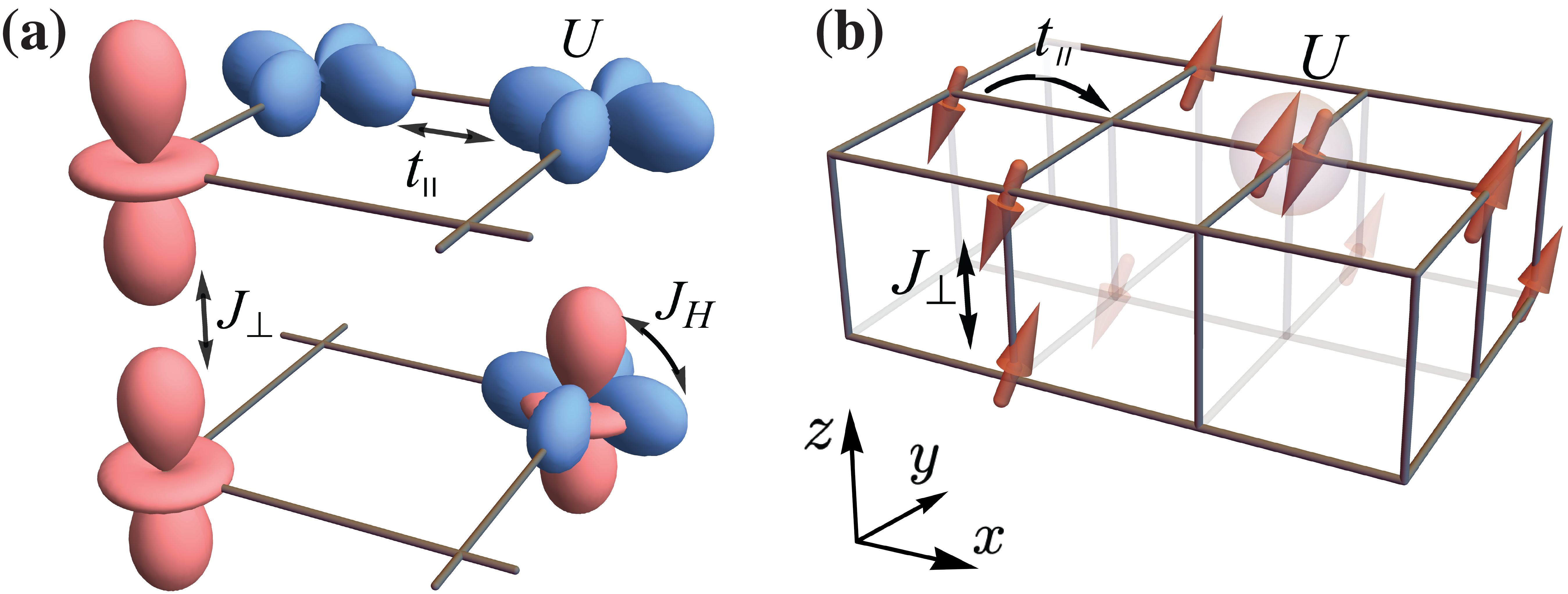
Figure 1: (a) Schematic representation of the low-lying two-orbital physics in LNO: the red $d_{z^{2}}$ orbital displays interlayer spin exchange coupling $J_{\perp}$, while the blue $d_{x^{2}-y^{2}}$ orbital features intralayer hopping term $t_{\|}$ as well as on-site Hubbard interaction $U$. The Hund’s coupling $J_{H}$ links these two orbitals. (b) Minimal model for $d_{z^{2}}$ orbital, applicable when $J_{H}$ is strong enough to align the spins between the $d_{x^{2}-y^{2}}$ and $d_{z^{2}}$ orbitals.

However, as we will show, the density matrix renormalization group (DMRG) results indicate that the on-site Hubbard interaction does indeed substantially enhance the pairing strength, particularly when the intermediate inter-layer spin exchange coupling is close to estimation from DFT calculations [5, 9, 10, 11, 12]. This numerical evidence offers a compelling hint that the Coulomb interaction itself still plays a significant role in the pairing mechanism. Based on this, we will further demonstrate that the motion of a single hole is severely restricted due to the accumulation of emergent $\mathbb{Z}_{2}$ Berry phases [illustrated in Fig. 3(a)], which arises from the restricted Hilbert space due to the strong on-site Hubbard interaction. Only the channel of inter-layer hole pairs on the background of inter-layer singlet spin pairs remains unvanished weight because the $\mathbb{Z}_{2}$ Berry phase can be fully canceled [shown in Fig. 3(b)]. This kinetic-energy-driven pairing mechanism originates directly from strong Coulomb repulsion, which is applicable across a wide range of hole doping concentrations and is not sensitive to other orbital specifics, such as particular inter-orbital couplings.

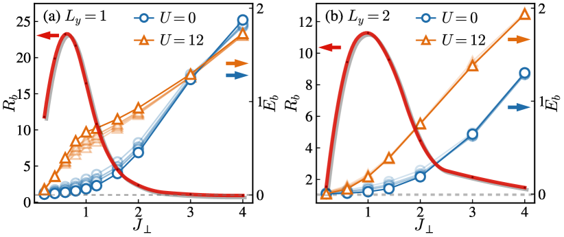
Figure 2: The binding energy $E_{b}$ for different on-site repulsion $U$ and the corresponding ratio $R_{b}$ as a function of interlayer coupling $J_{\perp}$ with $L_{y}=1,2$ for panel (a) and (b), respectively. The system length is $L_{x}=8,12,16,32$ for markers of decreasing transparency. The hole doping is fixed at $\delta=1/2$. The horizontal dashed lines mark $R_{b}=1$ and $E_{b}=0$.

Binding energy from Hubbard repulsion.— Start with the minimal model describing the $d_{x^{2}-y^{2}}$ orbital with filling $\nu\approx 1/4$, as specified by [cf. Fig. 1(b)]:

$$H_{t_{\|}\text{-}U\text{-}J_{\perp}} = -t_{\|}\sum_{\langle ij\rangle\alpha\sigma}\left(c_{i\alpha\sigma}^{\dagger}c_{j\alpha\sigma}+\text{ h.c.}\right)-\mu\sum_{i\alpha\sigma}n_{i\alpha\sigma}$$ (1)

$$+U\sum_{i\alpha}n_{i\alpha\uparrow}n_{i\alpha\downarrow}+J_{\perp}\sum_{i}\bm{S}_{i1}\cdot\bm{S}_{i2},$$

where $\sigma=\uparrow,\downarrow$ is the spin orientation, and $\alpha=1,2$ denotes the layer index. $\bm{S}_{i\alpha}$ and $n_{i\alpha\sigma}=c_{i\alpha\sigma}^{\dagger}c_{i\alpha\sigma}$ are the local SU(2) spin operator and electron number operator, respectively. Note that the $d_{x^{2}-y^{2}}$ orbital exhibits negligible interlayer single-particle tunneling, implying that the interlayer spin exchange coupling is expected to be ignored as well. However, one can interpret the in Eq. (1) as mediated through strong Hund’s coupling[shown in Fig. 1(a)], facilitated by interlayer spin exchange coupling in the $d_{z^{2}}$ orbital, which is nearly Mott localization due to $\nu\approx 1/2$.

Firstly, we investigate the strongly correlated effect in the bilayer $t_{\|}$-$U$-$J_{\perp}$ model in Eq. (1) using DMRG method on a bilayer lattice of size $L_{x}\times L_{y}$ with $L_{y}$ being the shorter side. The total number of sites is $N=L_{x}\times L_{y}\times L_{z}$ with $L_{z}=2$. We keep the bond dimension up to $5000$ with a typical truncation error $\epsilon\lesssim 10^{-7}$. The binding energy of holes is defined as

$$E_{b}=2E(N_{h}+1)-E(N_{h}+2)-E(N_{h}),$$ (2)

where $E(N_{h})$ denotes the ground state energy with the fixed number of doped holes $N_{h}=N\delta$. The total spin $S^{z}$ is fixed at $0$ and $1/2$ for even and odd numbers of holes respectively. Note that the binding energy has an overall linear dependence of $J_{\perp}$ since the Hamiltonian scales with $J_{\perp}$. Hence, we define a dimensionless ratio

$$R_{b}=\frac{E_{b}(U=12)}{E_{b}(U=0)},$$ (3)

to reflect the enhancement of binding energy caused by the Hubbard repulsion. The value of $R_{b}$ for different $J_{\perp}$ is depicted by the red lines in Fig. 2, which shows a significant enhancement in binding energy due to on-site repulsion $U$ in both cases of $L_{y}=1$ and $L_{y}=2$. Notably, this effect is most pronounced when the interlayer coupling $J_{\perp}$ is relatively small, specifically when $J_{\perp}\lesssim t_{\parallel}$, which is in line with the realistic values obtained through DFT calculations. Certainly, such a huge amplification of binding energy still necessitates the assistance of a finite interlayer coupling, albeit not excessively so. This is because at doping $\delta=1/2$, neither the Hubbard chain nor the two-leg Hubbard ladder is a quasi-one-dimensional superconducting state (as the Luther-Emery liquid), which is consistent with the vanishing binding energy at $J_{\perp}\rightarrow 0$ shown in Fig. 2. One is referred to Supplemental Material [27] for numerical evidences from more observables such as pair-pair correlators.

Therefore, when contemplating pairing mechanisms, strong Coulomb repulsion should itself be regarded as a non-negligible factor, rather than simply a contributor to spin-exchange interactions.

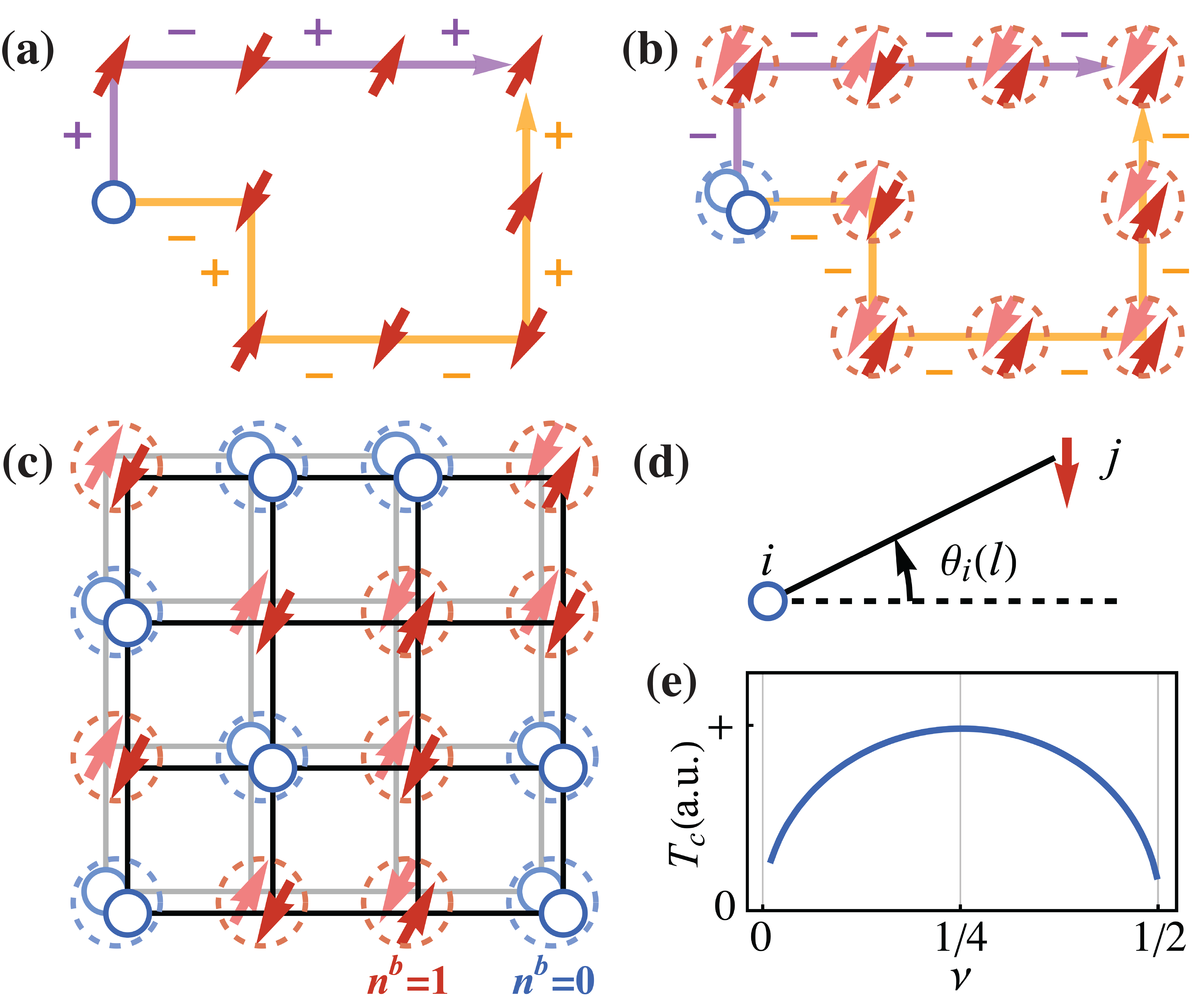
Figure 3: (a)-(b) Depiction of the $\mathbb{Z}_{2}$ Berry phase experienced by single holes in (a) and hole pairs set against the backdrop of spin-singlet pairs in (b). Dark (light) blue circles indicate holes in the 1st (2nd) layer, while dark (light) red arrows represent spins in the 1st (2nd) layer. (c) Schematic outline of the effective hard-core bosonic model, as given by Eq. (8): Spin-singlet pairs enclosed by red dashed circles correspond to $n^{b}_{i}=1$ state, states, and hole pairs enclosed by blue dashed circles correspond to $n^{b}_{i}=0$ states. (d) Graphic representation of the unitary transformation $e^{i\hat{\Theta}}$ as defined in Eq. (7) in the two-dimensional case. (e)Superconducting $T_{c}$ versus filling $\nu$ obtained by effective model Eq. (8) at the mean-field level, with $J_{\perp}=0.6t_{\|}$ and $J_{\|}=2J_{\perp}/3$.

Emergent $\mathbb{Z}_{2}$ Berry phases.— In the following, we consider the regime where $U\gg t_{\|}$, in which the states with double occupancy are energetically unfavorable and can be effectively projected out. The projection operator is denoted as $\hat{\mathcal{P}}$. This results in the $H_{t_{\|}\text{-}J_{\|}\text{-}J_{\perp}}$ model [28, 29, 30], derived from Eq. (1) as follows:

$$\begin{split}&H_{t_{\|}\text{-}J_{\|}\text{-}J_{\perp}}=-t_{\|}\sum_{\langle ij\rangle\alpha\sigma}\hat{\mathcal{P}}\left(c_{i\alpha\sigma}^{\dagger}c_{j\alpha\sigma}+\text{ h.c.}\right)\hat{\mathcal{P}}\\ &-\mu\sum_{i\alpha\sigma}n_{i\alpha\sigma}+J_{\|}\sum_{\langle ij\rangle\alpha}\bm{S}_{i\alpha}\cdot\bm{S}_{j\alpha}+J_{\perp}\sum_{i}\bm{S}_{i1}\cdot\bm{S}_{i2},\end{split}$$ (4)

where the intralayer coupling $J_{\|}$ denotes the intralayer spin exchange coupling. Based on DFT calculations [5, 9, 10, 11, 12], we find $J_{\perp}\approx 0.6t_{\|}$, $J_{\|}\approx 2J_{\perp}/3$, and the filling is $\nu\approx 1/4$. The Hilbert space is restricted by the no-double-occupancy constraint $\sum_{\sigma}n_{i\alpha\sigma}\leqslant 1$ at each site. This constraint, originating from the strong local Coulomb repulsion, introduces a non-trivial sign structure (refer to $\tau_{C}$) in the partition function $Z_{t_{\|}-J_{\|}-J_{\perp}}$:

$$Z_{t_{\|}\text{-}J_{\|}\text{-}J_{\perp}}\equiv\operatorname{Tr}e^{-\beta H_{t_{\|}\text{-}J_{\|}\text{-}J_{\perp}}}=\sum_{C}\tau_{C}W_{t_{\|}\text{-}J_{\|}\text{-}J_{\perp}}[C],$$ (5)

where $\beta$ is the inverse temperature, and $W_{t_{\|}\text{-}J_{\|}\text{-}J_{\perp}}[C]\geqslant 0$ denotes the non-negative weight corresponding to each closed loop $C$ of hole hopping paths on the square lattice. The sign factor $\tau_{C}$ associated with each closed loop $C$ is rigorously defined as follows [27]:

$$\tau_{C}\equiv(-1)^{N^{h}_{\mathrm{ex}}}\times(-1)^{N^{h}_{\downarrow}},$$ (6)

in which $N^{h}_{\mathrm{ex}}$ represents the total number of exchanges between identical holes, akin to the Fermi statistical sign structure found in doped semiconductors. Notably, the term $(-1)^{N^{h}_{\downarrow}}$ in Eq. (6) is identified as the phase-string [31, 32, 33], in which $N^{h}_{\downarrow}$ accounts for the total number of mutual exchanges between holes and down-spins. In other words, as illustrated in Fig. 3(a), the act of hole hopping can accumulate a $\mathbb{Z}_{2}$ Berry phase with its sign determined by the direction of the spin that is exchanged—positive for spin-up and negative for spin-down. It is crucial to emphasize that this emergent $\mathbb{Z}_{2}$ nature is an exclusive consequence of strong Coulomb repulsion and is not contingent on the specific details of the model. Consequently, this finding is broadly applicable to other strongly correlated systems, such as the single-layer $t$-$J$ model with extended coupling [33, 34], or the Hubbard model defined on arbitrary lattices [35, 36].

Therefore, the mobility of a single hole is significantly suppressed due to destructive interference effects among various [shown in Fig. 3(a)], as formulated in the path integral framework. This theoretical insight is corroborated by DMRG calculations, which show a rapid decay in the single-particle Green’s function $G_{\alpha\sigma}(r)=\langle c_{i,\alpha\sigma}^{\dagger}c_{j+r\hat{x},\alpha\sigma}\rangle$ upon turning on the Hubbard term $U$, as illustrated in Fig. 4(a) [27].

On the other hand, this $\mathbb{Z}_{2}$ frustration can be fully canceled when two holes from distinct layers pair and move together on a background of spin-singlet interlayer pairs, as depicted in Fig. 3(b). In such configurations, each exchange involving the two-hole composite and spin-singlet consistently contributes a negative sign, which ultimately cancels out upon completing a closed loop on a bipartite lattice. This phenomenon promotes pairing between interlayer charge (and spin) degrees of freedom, thereby steering the system towards a SC state.

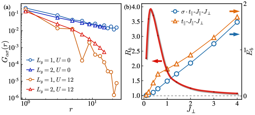
Figure 4: (a) The single-particle Green’s function $G_{\alpha\sigma}(r)$ for different on-site repulsion $U$ with $J_{\perp}/t_{\|}=0.6$ for $L_{y}=1$ and $J_{\perp}/t_{\|}=1.4$ for $L_{y}=2$. (b) The binding energy $E_{b}$ for the $t_{\|}$-$J_{\|}$-$J_{\perp}$ model and $\sigma\cdot t_{\|}$-$J_{\|}$-$J_{\perp}$ model and the corresponding ratio $R_{b}$ as a function of inter-layer coupling $J_{\perp}$ with $J_{\|}/t_{\|}=1/3$ and system length $L_{x}=32$. The hole doping is fixed at $\delta=1/2$. The horizontal dashed lines mark $R_{b}=1$ and $E_{b}=0$.

To more explicitly elucidate the physical implications of this unique correlation between hopping holes and background spins, as mediated by the emergent $\mathbb{Z}_{2}$ Berry phase, we can employ a unitary transformation [37, 38]

$$e^{i\hat{\Theta}}\equiv\exp\left(-i\sum_{i\alpha}n_{i\alpha}^{h}\hat{\Omega}_{i\alpha}\right),$$ (7)

on the original Hamiltonian Eq. (4). Here, $n_{i\alpha}^{h}=1-\sum_{\sigma}c_{i\alpha\sigma}^{\dagger}c_{i\alpha\sigma}$ denotes a local number of the hole at the site $i$ of layer $\alpha$. Additionally, $\hat{\Omega}_{i\alpha}$ accounts for the relative position between the hole $n_{i\alpha}^{h}$ and all other spins within the same layer $\alpha$.

To simplify our discussion, we initially focus on the one-dimensional limit, specifically a two-leg chain with $L_{y}=1$ as illustrated in Fig. 1(b). In this case, we define $\hat{\Omega}_{i\alpha}^{\text{1D}}=\pi\sum_{l>i}n_{l\alpha}^{\downarrow}$. Upon performing a unitary transformation, the original Hamiltonian would be transformed as $e^{-i\hat{\Theta}}H_{t_{\|}\text{-}J_{\|}\text{-}J_{\perp}}e^{i\hat{\Theta}}=H_{\sigma t_{\|}\text{-}J_{\|}\text{-}J_{\perp}}+H_{\text{string}}$, where $H_{\sigma t_{\|}\text{-}J_{\|}\text{-}J_{\perp}}$ is the same as $H_{t_{\|}\text{-}J_{\|}\text{-}J_{\perp}}$ in Eq. (4), except that the sign of hopping integral depends on the spin direction, i.e., $-t_{\|}c_{i\alpha\sigma}^{\dagger}c_{j\alpha\sigma}\rightarrow-\sigma t_{\|}c_{i\alpha\sigma}^{\dagger}c_{j\alpha\sigma}$, which explicit remove the sign frustration shown in Eq. (6) [27]. However, the cost needed to pay is the additional part $H_{\text{string}}=J_{\perp}/2\sum_{i}\left(\bm{S}_{i1}^{+}\bm{S}_{i2}^{-}+\bm{S}_{i1}^{-}\bm{S}_{i2}^{+}\right)\left(\Lambda_{i}^{h}-1\right)$, with the string term $\Lambda_{i}^{h}\equiv\exp\left[i\pi\sum_{l<i}\left(n_{l1}^{h}-n_{l2}^{h}\right)\right]$ characterizes the nonlocal phase shift effects arising from spatially separated holes on both chains (more details in Ref. 39 and SM [27]). Since the expectation value of transverse spin at each rung is given by $\langle\bm{S}_{i1}^{+}\bm{S}_{i2}^{-}+\bm{S}_{i1}^{-}\bm{S}_{i2}^{+}\rangle<0$ (denoted by $-g_{0}$), as ensured by short-range AFM correlation via the coupling $J_{\perp}$, one finds that two holes at the distinct chain with the coordinate $r_{\alpha=1}$ and $r_{\alpha=2}^{\prime}$ will generally acquire a linearly dependent pairing potential $V_{\text{string}}\sim J_{\perp}g_{0}\left|r_{\alpha=1}-r_{\alpha=2}^{\prime}\right|$. Crucially, such pairing potential can be validated by comparing the binding energy in the $t_{\|}$-$J_{\|}$-$J_{\perp}$ and $\sigma t_{\|}$-$J_{\|}$-$J_{\perp}$ models through DMRG calculations. The results in Fig. 4(b) unambiguously indicate stronger binding in the $t_{\|}$-$J_{\|}$-$J_{\perp}$ model, particularly around the experimental relevant regime where $J_{\perp}/t\sim 0.6$ [5, 9, 10, 11, 12].

Furthermore, all the above derivation can be extended to two-dimensional, i.e., restore $L_{y}\rightarrow\infty$ in Fig. 1(b), by setting $\hat{\Omega}_{i\alpha}^{\text{2D}}=\sum_{l\neq i}\theta_{i}(l)n_{l\alpha}^{\downarrow}$ in Eq. (7), which is depicted in Fig. 3(d). Here, $\theta_{i}(l)\equiv\pm\operatorname{Im}\ln\left(z_{i}-z_{l}\right)$ with $z_{i}$ denoting the complex coordinate of site $i$. Similarly, the interlayer spin-flip term can also induce a strong pairing potential $V_{\text{string}}\sim J_{\perp}g_{0}\left|r_{\alpha=1}-r_{\alpha=2}^{\prime}\right|^{2}$ between two holes at distinct layer [27]. It is noteworthy that the distinguishing feature of this additional pairing mechanism from traditional spin-exchange pairing lies in its string-like long-range interaction, which means that it does not necessarily require a very strong spin coupling $J_{\perp}$ to bind holes. Furthermore, while the hopping term in two dimensions under the unitary transformation Eq. (7) includes additional, more complex terms compared to the one-dimensional $\sigma t$ term, it is important to note that these complexities do not substantially affect our preceding arguments.

Effective Model.— Building on these physical implications, holes across distinct layers are inclined to form tightly bound 2e-charge bosons (blue dashed circles in Fig. 3(c)) due to a hidden confinement potential from the $\mathbb{Z}_{2}$ Berry phase in systems exhibiting short-range AFM correlations. At the same time, spins are predisposed to form singlet pairs across interlayers, resulting in neutral bosons with $S=0$ (red dashed circles in Fig. 3(c)), as a result of the interlayer AFM exchange coupling $J_{\perp}$.

Therefore, one can define the $b$-boson as the interlayer singlet pairs of bare electrons, with the correspondence $b_{i}=\frac{1}{\sqrt{2}}(c_{i1\uparrow}c_{i2\downarrow}-c_{i1\downarrow}c_{i2\uparrow})$. The local number of hardcore $b$-boson (local pairs) $\hat{n}_{i}^{b}=b_{i}^{\dagger}b_{i}$ cannot take the value larger than unity due to the no-double-occupancy-constraint of Eq. (4). Then, with the standard Brillouin-Wigner perturbation theory, the original Hamiltonian Eq. (4) can be reduced to the low-energy Hilbert subspace $\mathcal{H}=\bigotimes_{i}\text{span}\{|0\rangle_{c},b_{i}^{\dagger}|0\rangle_{c}\}$, thereby the effective Hamiltonian for hard-core boson is given by [27]:

$$H_{\text{eff}}=-w\sum_{\langle ij\rangle}\left(b_{i}^{\dagger}b_{j}+\text{h.c.}\right)-V\sum_{\langle ij\rangle}\hat{n}_{i}^{b}\hat{n}_{j}^{b}-\lambda\sum_{i}\hat{n}_{i}^{b}$$ (8)

where $w=8t_{\|}^{2}/3J_{\perp}$ denotes effective hopping term for boson, $V=J_{\|}^{2}/8J_{\perp}$ denotes a weak neighbouring attractive interaction with the strength $V\ll w$, as $t_{\|}\gg J_{\|}$ in Eq. (4), and $\lambda=3J_{\perp}/4+2\mu$ is the chemical potential associated with the fillings $\nu$.

The effective model $H_{\text{eff}}$ in Eq. (8) describes a single-layer hard-core Bose system with a weak nearest-neighbor attractive interaction, as shown in Fig. 3(c). In one dimensional scenario, $H_{\text{eff}}$ simplifies to a single chain and can be analytically solved using the bosonization method after applying the Jordan-Wigner transformation (cf. SM [27]). This results in a Luther-Emery liquid in the superconducting (SC) phase, characterized by an SC exponent $K_{\text{SC}}<1$, when the nearest-neighbor interaction is attractive, i.e., $V>0$.

In the two-dimensional context, the mean-field order parameter $\langle b_{i}\rangle=\sqrt{\rho_{s}}$ serves to decouple the effective Hamiltonian $H_{\text{eff}}$ in Eq. (8), reducing it to the independent local Hilbert space $\mathcal{H}$ [27]. For a giving filling $\nu$, the mean-field order parameter $\rho_{s}$ is self-consistently determined. Our findings indicate that the $b$-bosons enter a superfluid phase with $\rho_{s}\neq 0$ at zero temperature unless the occupancy number $2\nu$ is an integer. In fact, this phase corresponds to the SC state in the original fermionic system, marked by the condensation of Cooper pairs. Furthermore, at finite temperature, the coherence of $b$-bosons would be disrupted by the thermal fluctuation, and then undergo a Kosterlitz-Thouless(KT) transition to restore the charge $U(1)$ symmetry at the critical temperature $T_{c}$. As a result, the SC phase transition temperature can be estimated by the KT temperature [40]

$$T_{c}=\pi w\rho_{s}=\frac{8\pi t_{\|}^{2}}{3J_{\perp}}\rho_{s},$$ (9)

of which the filling dependence is shown in Fig. 3(e). Our results indicate that $T_{c}$ peaks precisely at $\nu=1/4$, aligning with the actual situation of the $d_{x^{2}-y^{2}}$ orbitals in LNO. In contrast, $T_{c}$ is drastically suppressed at $\nu=1/2$, a condition corresponding to the undoped featureless Mott insulator, also known as a symmetric mass generation (SMG) insulator [41, 42, 43, 44, 45].

Discussion.— In this work, the pairing mechanism in novel high-$T_{c}$ SC material $\mathrm{La}_{3}\mathrm{Ni}_{2}\mathrm{O}_{7}$ has been explored, in which a significant role of the Coulomb repulsion $U$ among $d$-orbital electrons has been revealed. Although a non-zero interlayer superexchange coupling $J_{\perp}$ is essential for the pairing, the binding energy is found to be strongly enhanced with $U$ tuned into the strong-coupling (Mott) limit as opposed to $U=0$. In the former regime (large $U$), the propagation of the single electron (hole) within each of the bilayer becomes severely frustrated due to the accumulation of a $\mathbb{Z}_{2}$ Berry phase (phase string). On the other hand, such $\mathbb{Z}_{2}$ phase frustration can be completely canceled out when two holes are paired up via $J_{\perp}$ such that the strong suppression of the kinetic energy can be effectively released. By contrast, artificially turning off this Berry phase, the binding is also suppressed even in the large $U$ case. It means that the pairing in the Mott regime is indeed substantially driven up by saving the kinetic energy [46, 47], with the magnitude of $\sim 10$-$20$ times bigger than simply by a bare $J_{\perp}\sim t_{\|}$ with $U=0$. The latter regime has been studied in other approaches  [10, 15, 16, 20, 21, 22, 23, 24, 25, 26, 19]. Although the latter mechanism may also yield a similar effective Hamiltonian $H_{\text{eff}}$ in Eq. (8) in the BEC limit [19], it generally requires an unrealistically large $J_{\perp}$, much exceeding the hopping term $t_{\|}$.

Moreover, at the high-temperature phase, the spin-singlet pairs are destroyed, leading to the strong $\mathbb{Z}_{2}$ Berry phase frustration that can be experienced by both single hole and hole pairs, resulting in a loss of coherence of the charge degrees of freedom in this phase. As discussed in the previous study [48], the scattering between holes and random phase (flux) can naturally give rise to a linear-$T$ dependence of electric resistivity, which is consistent with the experimental measurement in LNO [6, 8, 5].

Supplementary Materials for: “Strong Pairing Originated from an Emergent $\mathbb{Z}_{2}$ Berry Phase in $\mathbf{La}_{3}\mathbf{Ni}_{2}\mathbf{O}_{7}$”

In the supplementary materials that follow, we offer additional analytical and numerical results to reinforce the conclusions put forth in the main text. In Section I, we present a rigorous derivation of the sign structure referred to in Eq.(6) for both the $t_{\|}$-$J_{\|}$-$J$ model and the $\sigma t_{\|}$-$J_{\|}$-$J$ model. Section II offers a comprehensive derivation of the effective attraction interaction, denoted as $V_{\text{string}}$, for both one-dimensional and two-dimensional scenarios. In Section III, we delve into the derivation of the effective model $H_{\text{eff}}$ as described in Eq. (8), and subsequently explore its physical implications in both one-dimensional and two-dimensional cases. In Section IV, we show more numerical evidences on the enhancement of pairing strength from the on-site repulsion.

Appendix A I. The Exact Sign Structure of the $t_{\|}\text{-}J_{\|}\text{-}J_{\perp}$ Hamiltonian

In this section, we provide a rigorous proof for the partition function described in Eq.(5) and elaborate on the sign structure referenced in Eq.(6). We initiate our discussion with the slave-fermion formalism. In this context, the electron operator is represented as $c_{i\alpha\sigma}=f_{i\alpha}^{\dagger}b_{i\alpha\sigma}$, where $f_{i\alpha}^{\dagger}$ refers to the fermionic holon operator and $b_{i\alpha\sigma}$ to the bosonic spinon operator. These relations are governed by the constraint $f_{i\alpha}^{\dagger}f_{i\alpha}+\sum_{\sigma}b_{i\alpha\sigma}^{\dagger}b_{i\alpha\sigma}=1$. To shed light on the sign structure inherent in this model, we incorporate the Marshall sign into the $S_{z}$-spin representation. This is achieved through the substitution $b_{i\alpha\sigma}\rightarrow(-\sigma)^{i+\alpha}b_{i\alpha\sigma}$, which leads to

$$c_{i\alpha\sigma}=(-\sigma)^{i+\alpha}f_{i}^{\dagger}b_{i\alpha\sigma}.$$ (AS1)

Consequently, the $\sigma t_{\|}\text{-}J_{\|}\text{-}J_{\perp}$ model is transformed as follows:

$$H_{t_{\|}\text{-}J_{\|}\text{-}J_{\perp}}=-t_{\|}\left(P_{o\uparrow}^{\|}-P_{o\downarrow}^{\|}\right)-\frac{J_{\|}}{4}\left(Q^{\|}+P_{\uparrow\downarrow}^{\parallel}\right)-\frac{J_{\perp}}{4}\left(Q^{\perp}+P_{\uparrow\downarrow}^{\perp}\right),$$ (AS2)

where

$$P_{o\uparrow}^{\parallel} = \sum_{\langle ij\rangle\alpha}b_{i\alpha\uparrow}^{\dagger}b_{j\alpha\uparrow}f_{j}^{\dagger}f_{i}+\text{h.c.},\;\;\;\;\;\;\;\;\;\;\;\;P_{o\downarrow}^{\parallel}=\sum_{\langle ij\rangle\alpha}b_{i\alpha\downarrow}^{\dagger}b_{j\alpha\downarrow}f_{j}^{\dagger}f_{i}+\text{h.c.},$$ (AS3)

$$P^{\parallel}_{\uparrow\downarrow} = \sum_{\langle ij\rangle\alpha}b_{i\alpha\uparrow}^{\dagger}b_{j\alpha\downarrow}^{\dagger}b_{i\alpha\downarrow}b_{j\alpha\uparrow}+\text{h.c.},\;\;\;\;\;\;P^{\perp}_{\uparrow\downarrow}=\sum_{i}b_{i1\uparrow}^{\dagger}b_{i2\downarrow}^{\dagger}b_{i1\downarrow}b_{i2\uparrow}+\text{h.c.},$$ (AS4)

$$Q^{\parallel} = \sum_{\langle ij\rangle\alpha}\left(n_{i\uparrow}n_{j\downarrow}+n_{i\downarrow}n_{j\uparrow}\right),\;\;\;\;\;\;\;\;\;\;\;\;\;\;Q^{\perp}=\sum_{i}\left(n_{i1\uparrow}n_{i2\downarrow}+n_{i1\downarrow}n_{i2\uparrow}\right)$$ (AS5)

The operators $P_{o\sigma}^{\|}$, $P_{\uparrow\downarrow}^{\|}$, and $P_{\uparrow\downarrow}^{\perp}$ represent the intralayer hole-spin nearest-neighbor (NN) exchange, intralayer NN spin superexchange, and interlayer NN spin superexchange, respectively. The terms $Q^{\|}$ and $Q^{\perp}$ correspond to potential interactions between NN spins. By utilizing the high-temperature series expansion, we derive the partition function up to all orders [33]

$$Z_{t_{\|}\text{-}J_{\|}\text{-}J_{\perp}} = \operatorname{Tr}e^{-\beta H_{t_{\|}\text{-}J_{\|}\text{-}J_{\perp}}}=\operatorname{Tr}\sum_{n=0}^{\infty}\frac{\beta^{n}}{n!}\left(-H_{t_{\|}\text{-}J_{\|}\text{-}J_{\perp}}\right)^{n}$$ (AS6)

$$= \sum_{n=0}^{\infty}\frac{(J_{\perp}\beta/4)^{n}}{n!}\operatorname{Tr}\left[\sum\ldots\left(\frac{4t_{\|}}{J_{\perp}}P^{\|}_{o\uparrow}\right)\ldots\left(\frac{J_{\|}}{J_{\perp}}Q^{\|}\right)\ldots P^{\perp}_{\uparrow\downarrow}\ldots\left(-\frac{4t_{\|}}{J_{\perp}}P_{o\downarrow}^{\|}\right)\ldots\left(\frac{J_{\|}}{J_{\perp}}P_{\uparrow\downarrow}^{\|}\right)\ldots Q^{\perp}\ldots\right]_{n}$$

$$= \sum_{n=0}^{\infty}(-1)^{N_{\downarrow}^{h}}\frac{(J_{\perp}\beta/4)^{n}}{n!}\operatorname{Tr}\left[\sum\ldots\left(\frac{4t_{\|}}{J_{\perp}}P^{\|}_{o\uparrow}\right)\ldots\left(\frac{J_{\|}}{J_{\perp}}Q^{\|}\right)\ldots P^{\perp}_{\uparrow\downarrow}\ldots\left(\frac{4t_{\|}}{J_{\perp}}P_{o\downarrow}^{\|}\right)\ldots\left(\frac{J_{\|}}{J_{\perp}}P_{\uparrow\downarrow}^{\|}\right)\ldots Q^{\perp}\ldots\right]_{n}$$

with the underlying assumption that the NN hopping integral remains positive, signified by $t_{\|}>0$. The notation $[\sum\ldots]_{n}$ encompasses the summation over all $n$-block production. Owing to the trace, both starting and ending configurations of holes and spins must coincide, ensuring that all contributions to $Z_{t_{\|}\text{-}J_{\|}\text{-}J_{\perp}}$ are delineated by closed loops of holes and spins. Within this framework, $N_{\downarrow}^{h}$ quantifies the exchanges between down-spins and holes. Then, we insert a complete Ising basis with holes, given by $\sum_{\phi\left\{l_{h}\right\}}\left|\phi;\left\{l_{h}\right\}\right\rangle\left\langle\phi;\left\{l_{h}\right\}\right|=1$, between operators inside the trace. Here, $\phi$ specifies the spin configuration, while $\left\{l_{h}\right\}$ indicates the positions of the holes. Therefore, the partition function can be written as a compact expression:

$$Z_{t_{\|}\text{-}J_{\|}\text{-}J_{\perp}}=\sum_{C}\tau_{C}W_{t_{\|}\text{-}J_{\|}\text{-}J_{\perp}}[C],$$ (AS7)

with relevant sign information is encapsulated by:

$$\tau_{C}^{t_{\|}\text{-}J_{\|}\text{-}J_{\perp}}\equiv(-1)^{N_{\mathrm{ex}}^{h}}\times(-1)^{N_{\downarrow}^{h}},$$ (AS8)

which aligns with Eq. (6) presented in the main text. In this context, $N_{\mathrm{ex}}^{h}$ represents the number of hole exchanges arising from the fermionic statistics of the holon $f$. This sign structure is comprehensively defined across varying doping levels, temperatures, and finite sizes for the $t_{\|}\text{-}J_{\|}\text{-}J_{\perp}$ model. Additionally, the non-negative weight $W[C]$ for a closed loop $C$ emerges from a sequence of positive elements within the trace of Eq. (AS6).

Furthermore, by introducing the $\sigma t_{|}\text{-}J_{|}\text{-}J_{\perp}$ model, where the intrinsic spin exchange term remains unchanged, but the hopping term in Eq.(4) is substituted by:

$$H_{\sigma t_{\|}}=-t_{\|}\sum_{\langle ij\rangle}\sigma c_{i\sigma}^{\dagger}c_{j\sigma}+\text{h.c.},$$ (AS9)

in which an additional spin-dependent sign, $\sigma$, is integrated into the NN hopping term, nullifying the “$-$” sign preceding the $P_{o\downarrow}$. As a result, the $\sigma t_{|}\text{-}J_{|}\text{-}J_{\perp}$ model, under the representation of Eq. (AS1), can be rewritten as:

$$H_{\sigma t_{\|}\text{-}J_{\|}\text{-}J_{\perp}}=-t_{\|}\left(P_{o\uparrow}^{\|}+P_{o\downarrow}^{\|}\right)-\frac{J_{\|}}{4}\left(Q^{\|}+P_{\uparrow\downarrow}^{\|}\right)-\frac{J_{\perp}}{4}\left(Q^{\perp}+P_{\uparrow\downarrow}^{\perp}\right),$$ (AS10)

with the partition function under the high-temperature series expansion expressed as::

$$Z_{\sigma t_{\|}\text{-}J_{\|}\text{-}J_{\perp}}=\sum_{n=0}^{\infty}\frac{(J_{\perp}\beta/4)^{n}}{n!}\operatorname{Tr}\left[\sum\ldots\left(\frac{4t_{\|}}{J_{\perp}}P^{\|}_{o\uparrow}\right)\ldots\left(\frac{J_{\|}}{J_{\perp}}Q^{\|}\right)\ldots P^{\perp}_{\uparrow\downarrow}\ldots\left(\frac{4t_{\|}}{J_{\perp}}P_{o\downarrow}^{\|}\right)\ldots\left(\frac{J_{\|}}{J_{\perp}}P_{\uparrow\downarrow}^{\|}\right)\ldots Q^{\perp}\ldots\right]_{n}$$ (AS11)

As the result, the sign structure for $\sigma t_{\|}\text{-}J_{\|}\text{-}J_{\perp}$ model is given by:

$$\tau_{C}^{\sigma t_{\|}\text{-}J_{\|}\text{-}J_{\perp}}=(-1)^{N_{\mathrm{ex}}^{h}},$$ (AS12)

in which the nontrivial phase string sign $(-1)^{N_{\downarrow}^{h}}$ vanishes.

Figure AS1: (a) Illustration of a certain configuration for holes(marked by blue) and spins(marked by red). $H_{\text{string}}$ vanishes at the blue rung, while it remains finite at the orange rung. (b) Sketch of positions of holes and spins on a two-layer system, with lighter(darker) color labeling the objects on the first(second) layer.

Appendix B II. Effective Attraction Interaction $V_{\text{string}}$ Obtained by Eq. (7)

In this section, more derivation details about the effective attraction interaction $V_{\text{string}}$ in the main text will be discussed for both the one-dimensional and two-dimensional cases.

B.1 II.A. One Dimensional Case

In the one-dimensional context, upon employing a unitary transformation $e^{i\hat{\Theta}}\equiv\exp\left(-i\sum_{i\alpha}n_{i\alpha}^{h}\hat{\Omega}_{i\alpha}\right)$ with $\hat{\Omega}_{i\alpha}^{1\mathrm{D}}=\pi\sum_{l>i}n_{l\alpha}^{\downarrow}$, the hopping term in $t_{\|}$-$J_{\|}$-$J_{\perp}$ model is given by:

$$e^{-i\hat{\Theta}}c_{i\alpha\sigma}^{\dagger}c_{i+1\alpha\sigma}e^{i\hat{\Theta}} = \exp\left[-i\sum_{j,\alpha}n_{j\alpha}^{h}\pi\sum_{l>j}n_{l\alpha}^{\downarrow}\right]c_{i\alpha\sigma}^{\dagger}c_{i+1\alpha\sigma}\exp\left[i\sum_{k,\alpha}n_{k\alpha}^{h}\pi\sum_{l>k}n_{l\alpha}^{\downarrow}\right]$$ (BS13)

$$= \exp\left[-i\sum_{j=i,i+1}\sum_{\alpha}n_{j\alpha}^{h}\pi\sum_{l>j}n_{l\alpha}^{\downarrow}\right]c_{i\alpha\sigma}^{\dagger}c_{i+1\alpha\sigma}\exp\left[i\sum_{k\neq i,i+1}\sum_{\alpha}n_{k\alpha}^{h}\pi\sum_{l>k}n_{l\alpha}^{\downarrow}\right]$$ (BS14)

$$= c_{i\alpha\sigma}^{\dagger}c_{i+1\alpha\sigma}\exp\left[-i\pi n_{i+1\alpha}^{\downarrow}\right]$$ (BS15)

$$= \sigma c_{i\alpha,\sigma}^{\dagger}c_{i+1\alpha\sigma}.$$ (BS16)

Similarly, the spin exchange interaction transforms as:

$$e^{-i\hat{\Theta}}\bm{S}_{i1}^{z}\bm{S}_{i2}^{z}e^{i\hat{\Theta}}=\exp\left[-i\sum_{j,\alpha}n_{j\alpha}^{h}\pi\sum_{l>j}n_{l,\alpha}^{\downarrow}\right]c_{i1\uparrow}^{\dagger}c_{i1\downarrow}c_{i2\downarrow}^{\dagger}c_{i2\uparrow}\exp\left[i\sum_{k,\alpha}n_{k\alpha}^{h}\pi\sum_{l>k}n_{l\alpha}^{\downarrow}\right]=\bm{S}_{i1}^{z}\bm{S}_{i2}^{z},$$ (BS17)

as well as:

$$e^{-i\hat{\Theta}}\bm{S}_{i1}^{+}\bm{S}_{i2}^{-}e^{i\hat{\Theta}} = \exp\left[-i\sum_{j,\alpha}n_{j\alpha}^{h}\pi\sum_{l>j}n_{l\alpha}^{\downarrow}\right]c_{i1\uparrow}^{\dagger}c_{i1\downarrow}c_{i2\downarrow}^{\dagger}c_{i2\uparrow}\exp\left[i\sum_{k,\alpha}n_{k\alpha}^{h}\pi\sum_{l>k}n_{l\alpha}^{\downarrow}\right]$$ (BS18)

$$= \exp\left[-i\sum_{j<i,\alpha}n_{j\alpha}^{h}\pi\sum_{l>j}n_{l\alpha}^{\downarrow}\right]c_{i1\uparrow}^{\dagger}c_{i1\downarrow}c_{i2\downarrow}^{\dagger}c_{i2\uparrow}\exp\left[i\sum_{k<i,\alpha}n_{k\alpha}^{h}\pi\sum_{\downarrow>k}n_{l\alpha}^{\perp}\right]$$ (BS19)

$$= \bm{S}_{i1}^{+}\bm{S}_{i2}^{-}\exp\left[i\pi\sum_{l<i}\left(n_{l1}^{h}-n_{l2}^{h}\right)\right].$$ (BS20)

As the result, combining Eq. (BS13), Eq. (BS17) and Eq. (BS18), the total Hamltonian $t_{\|}$-$J_{\|}$-$J_{\perp}$ can be expressed as:

$$e^{-i\hat{\Theta}}H_{t_{\|}-J_{\|}-J_{\perp}}e^{i\hat{\Theta}}=H_{\sigma t_{\|}-J_{\|}-J_{\perp}}+H_{\text{string}}.$$ (BS21)

Here, $H_{\sigma t_{\|}-J_{\|}-J_{\perp}}$ and $H_{\text{string }}$ are defined as:

$$H_{\sigma t_{\|}-J_{\|}-J_{\perp}} = -t_{\|}\sum_{\langle ij\rangle\alpha\sigma}\left(\sigma c_{i\alpha\sigma}^{\dagger}c_{j\alpha\sigma}+\text{ h.c. }\right)-\mu\sum_{i\alpha\sigma}n_{i\alpha\sigma}+J_{\|}\sum_{\langle ij\rangle\alpha}\bm{S}_{i\alpha}\cdot\bm{S}_{j\alpha}+J_{\perp}\sum_{i}\bm{S}_{i1}\cdot\bm{S}_{i2}$$ (BS22)

$$H_{\text{string }} = \frac{J_{\perp}}{2}\sum_{i}\left(\bm{S}_{i1}^{+}\bm{S}_{i2}^{-}+\bm{S}_{i1}^{-}\bm{S}_{i2}^{+}\right)\left(\Lambda_{i}^{h}-1\right)$$ (BS23)

with $\Lambda_{i}^{h}=\exp\left[i\pi\sum_{l<i}\left(n_{l1}^{h}-n_{l2}^{h}\right)\right]$. Here, Eq. (BS22) is the $\sigma t_{\|^{-}}J_{\|^{-}}J_{\perp}$ model with only the fermionic statistic sign, as depicted in Eq. (AS12). Furthermore, given the expectation value of the transverse spin at each rung by $\langle\bm{S}_{i1}^{+}\bm{S}_{i2}^{-}+\bm{S}_{i1}^{-}\bm{S}_{i2}^{+}\rangle<0$ (denoted by $-g_{0}$), it becomes evident that Eq. (BS23) vanishes when hole pairs across the rung exist on a background where spins also establish interchain singlet pairing. Nonetheless, when these hole pairs are broken and the two holes are separated by some distance, every rung with spin singlet pairs located between these holes will contribute $J_{\perp}g_{0}/2$ (highlighted by orange shadows in Fig. AS1(a)). This results in an energy cost that depends linearly:

$$V_{\text{string }}\sim J_{\perp}g_{0}\left|r_{\alpha=1}-r_{\alpha=2}^{\prime}\right|,$$ (BS24)

where $r_{\alpha=1}$ and $r_{\alpha=2}^{\prime}$ denote the coordinates of the holes on chain 1 and chain 2, respectively.

B.2 II.B. Two Dimensional Case

In the two dimensional case, the unitary transformation can be generalized by setting $\hat{\Omega}_{i\alpha}^{2\mathrm{D}}=\sum_{l\neq i}\theta_{i}(l)n_{l\alpha}^{\downarrow}$. With this transformation, the spin exchange term evolves as:

$$e^{-i\hat{\Theta}}\bm{S}_{i1}^{+}\bm{S}_{i2}^{-}e^{i\hat{\Theta}}=\bm{S}_{i1}^{+}\bm{S}_{i2}^{-}\exp\left[i\sum_{l\neq i}\theta_{i}(l)\left(n_{l1}^{h}-n_{l2}^{h}\right)\right].$$ (BS25)

When spin singlets form across the two layers, i.e., $\left\langle S_{i1}^{+}S_{i2}^{-}\right\rangle<0$, the ensuing energy cost from this term can be expressed as:

$$V_{\text{string}} = \left\langle\frac{J_{\perp}}{2}\sum_{i}e^{-i\hat{\Theta}}\left(\bm{S}_{i1}^{+}\bm{S}_{i2}^{-}+\bm{S}_{i1}^{-}\bm{S}_{i2}^{+}\right)e^{i\hat{\Theta}}-\frac{J_{\perp}}{2}\sum_{i}\left(\bm{S}_{i1}^{+}\bm{S}_{i2}^{-}+\bm{S}_{i1}^{-}\bm{S}_{i2}^{+}\right)\right\rangle$$ (BS26)

$$= -J_{\perp}g_{0}\sum_{i}\cos\left[i\sum_{l\neq i}\theta_{i}(l)\left(n_{l1}^{h}-n_{l2}^{h}\right)\right]+\sum_{i}Jg_{0}$$ (BS27)

$$\approx \frac{J_{\perp}g_{0}}{2}\int_{0}^{\infty}rdr\int_{0}^{2\pi}d\theta\phi^{2}+E_{\text{core}}$$ (BS28)

$$\varpropto J_{\perp}g_{0}\ln R\left|r_{\alpha=1}-r_{\alpha=2}^{\prime}\right|^{2}+E_{\text{core }},$$ (BS29)

where $R$ is the sample size, and $E_{\text{core }}$ represents the ultraviolet energy in proximity to the hole pairs. In the last line of Eq. (BS26), the relation $\phi\simeq|r_{\alpha=1}-r_{\alpha=2}^{\prime}|\sin\theta/l$ is used, and the definition of $\phi$, $l$ and $\theta$ is illustrated in Fig. AS1(b). It is noteworthy that the string tension $\ln R$ in Eq. (BS26) approaches infinity as we tend towards the thermodynamic limit. However, the term $g_{0}\ln R$ aims to remain finite, thereby avoiding energy divergence.

Appendix C III. Effective Model $H_{\text{eff}}$ in Eq. (8)

In this section, more derivation about $H_{\text{eff}}$ in Eq. (8) will be given, and then we will discuss its physical implication using the one-dimensional Abelian bosonization approach and the two-dimensional mean-field theory, respectively.

From our preceding discussions, the local Hilbert space at the $i$th rung of the original double-layer system can be divided into two subspaces with distinct energy scale:

• low-energy sector $\mathcal{V}_{0}$:

  $$|00\rangle_{i} : E=0$$ (CS30)

  $$\frac{1}{\sqrt{2}}(|\uparrow\downarrow\rangle_{i}-|\downarrow\uparrow\rangle_{i}) : E=-\frac{3}{4}J_{\perp}$$ (CS31)

• high-energy sector $\mathcal{V}_{1}$:

  $$|\downarrow\downarrow\rangle_{i},\;\;\;\;|\uparrow\uparrow\rangle_{i},\;\;\;\;\frac{1}{\sqrt{2}}(|\uparrow\downarrow\rangle_{i}+|\downarrow\uparrow\rangle_{i}) : E=\frac{1}{4}J_{\perp}$$ (CS32)

  $$|\downarrow 0\rangle_{i},\;\;\;\;|\uparrow 0\rangle_{i},\;\;\;\;|0\downarrow\rangle_{i},\;\;\;\;|0\uparrow\rangle_{i} : E=V_{\text{string }}$$ (CS33)

Then, we can define projective operators $P$ onto the low-energy sector $\mathcal{V}_{0}$ as follow:

$$P=\prod_{i}\sum_{\alpha\in V_{0}}|\alpha\rangle\langle\alpha|,$$ (CS34)

and projective operators $Q$ onto the high-energy sector $\mathcal{V}_{1}$;

$$Q=1-P.$$ (CS35)

Applying the Brillouin-Wigner perturbation theory, the effective Hamiltonian is given by: $H_{\mathrm{eff}}(E)=PHP-PHQ(QHQ-E)^{-1}QHP$. At the zeroth order, it becomes:

$$PH_{\sigma t_{\|}-J_{\|}-J_{\perp}}P=-\frac{3}{4}J_{\perp}\sum_{i}n_{i}^{b}-2\mu\sum_{i}n_{i}^{b},$$ (CS36)

where $n_{i}^{b}=b_{i}^{\dagger}b_{i}$ denotes the local number operator for hard-core boson, with the correspondence $b_{i}=\frac{1}{\sqrt{2}}\left(c_{i1\uparrow}c_{i2\downarrow}-c_{i1\downarrow}c_{i2\uparrow}\right)$. For the hopping term, the second-order virtual process is expressed as:

$$PH_{t_{\|}}Q(E-QHQ)^{-1}QH_{t_{\|}}P=-\frac{8t_{\|}^{2}}{3J_{\perp}+4V_{\text{string}}}\left(b_{i}^{\dagger}b_{j}+h.c.\right).$$ (CS37)

Similarly, for the intralayer spin exchange interactions, the second-order virtual process is given by:

$$PH_{J_{\|}}Q(E-QHQ)^{-1}QH_{J_{\|}}P=-\frac{J_{\|}^{2}}{8J_{\perp}}n_{i}^{b}n_{j}^{b}.$$ (CS38)

As the result, combining Eq. (CS36),Eq. (CS37) and Eq. (CS38), the resulting effective Hamltonian is given by:

$$H_{\mathrm{eff}}=\sum_{i}-w\left(b_{i}^{\dagger}b_{j}+\text{ h.c. }\right)-V\hat{n}_{i}^{b}\hat{n}_{j}^{b}-\lambda\hat{n}_{i}^{b},$$ (CS39)

which is consitent of Eq. (8) in the main text. Here, $w\approx 8t_{\|}^{2}/3J_{\perp}$ denotes effective hopping term for boson, $V=J_{\|}^{2}/8J_{\perp}$ denotes a weak neighbouring attractive interaction and $\lambda=3J_{\perp}/4+2\mu$ is the chemical potential associated with the fillings $\nu$. Note that $V_{\text{string}}$ here becomes negligible when the separation distance is very short (only a lattice constant in this case).

C.1 III.A. One Dimensional Case: Bosonization

For the one-dimensional scenario, the effective Hamiltonian, denoted by Eq. (8), can be expressed as:

$$H[\psi]=-w\sum_{i}\left(\psi_{i}^{\dagger}\psi_{i+1}+\psi_{i+1}^{\dagger}\psi_{i}\right)-V\sum_{i}n_{i}^{b}n_{i+1}^{b}-\lambda\sum_{i}n_{i}^{b}$$ (CS40)

under the Jordan-Wigner transformation:

$$\psi_{i}=b_{i}\exp\left(-i\pi\sum_{l>i}n_{i}\right).$$ (CS41)

Upon employing standard Abelian bosonization, the relationship between the fermionic and bosonic fields is

$$\psi_{i}=\frac{\eta}{\sqrt{2\pi a}}e^{ik_{b}x}e^{-i\left(\phi_{b}-\theta_{b}\right)}+\frac{\bar{\eta}}{\sqrt{2\pi a}}e^{-ik_{b}x}e^{-i\left(-\phi_{b}-\theta_{b}\right)}.$$ (CS42)

Consequently, the fermionic Hamiltonian, denoted Eq. (CS40), transforms to:

$$H[\phi,\theta]=\frac{u_{b}}{2\pi}\int dx\left\{K_{b}\left[\partial_{x}\theta_{b}(x)\right]^{2}+\frac{1}{K_{b}}\left[\partial_{x}\phi_{b}(x)\right]^{2}\right\}-\frac{U}{\pi}\partial_{x}\phi_{b},$$ (CS43)

which illustrates the low-energy fluctuations of the pairing field, $\phi$, with the stiffness constant:

$$K_{b}=1+V\frac{2\sin^{2}k_{F}}{\pi u_{b}}>1,$$ (CS44)

where $k_{F}=2\pi\nu$ signifies the effective Fermi momentum. Additionally, the density-density correlation with the hole number operator, denoted by $n^{h}_{i}=1-\sum_{\alpha\sigma}n_{i\alpha\sigma}/2$, is:

$$\left\langle n^{h}_{i}n^{h}_{i+r}\right\rangle=\left\langle n_{i}^{b}n_{i+r}^{b}\right\rangle\sim\frac{2}{(2\pi)^{2}}|r|^{-2K_{b}}\cos\left(2k_{F}r\right),$$ (CS45)

where the expression for the density operator is given by $n_{x}^{b}=-\frac{1}{\pi}\partial_{x}\phi_{b}+\frac{1}{2\pi}\left[e^{i2k_{b}x}e^{-2i\phi_{b}}+\text{ h.c. }\right]$. As the result, from Eq. (CS45), we deduce that the charge density exponent is $K_{C}=2K_{b}$. Moreover, the singlet superconducting pairing correlation, $\left\langle b_{i}b_{i+r}^{\dagger}\right\rangle$ in the fermionic representation is:

$$\left\langle b_{i}b_{i+r}^{\dagger}\right\rangle=\left\langle\exp\left(-i\pi\sum_{l>i}\hat{n}_{l}\right)\psi_{i}\psi_{i+r}^{\dagger}\exp\left(+i\pi\sum_{l>i+r}\hat{n}_{l}\right)\right\rangle\sim e^{ik_{F}r}|r|^{-(1/2)K_{b}^{-1}},$$ (CS46)

so that $K_{SC}=\frac{1}{2}K_{b}^{-1}$. A key observation is that $K_{C}K_{SC}=1$, which characterizes a Luther-Emery liquid. Notably, for $V>0$ indicating an attractive interaction, $K_{b}>1$ from Eq. (CS44) implies a heightened SC instability with $K_{SC}<1$.

C.2 III.B. Two Dimensional Case: Mean-Field Theory

In the two-dimensional case, the Hilbert space for distinct sites can be decoupled using the mean field ansatz, $\left\langle b_{i}\right\rangle=\sqrt{\rho_{s}}$, when starting from the effective Hamiltonian Eq. (8). The resulting mean-field(MF) Hamiltonian becomes:

$$H_{\text{MF}}=\sum_{i}\left[-s\left(b_{i}^{\dagger}+b_{i}\right)-vn_{i}^{b}+\epsilon\right]$$ (CS47)

with

$$s=\frac{32}{3J_{\perp}}t_{\|}^{2}\sqrt{\rho_{s}},\;\;\;\;\;v=\frac{J_{\|}^{2}}{2J_{\perp}}\rho_{s}+\frac{3}{4}J_{\perp}+2\mu,\;\;\;\;\;\;\;\epsilon=\frac{32}{3J_{\perp}}t_{\|}^{2}\rho_{s}+\frac{J_{\|}^{2}}{4J_{\perp}}\rho_{s}^{2}.$$ (CS48)

By diagonalizing this two-dimensional on-site Hilbert space, we acquire the local ground state $|\text{GS}\rangle_{i}$ and its corresponding energy $E_{\text{GS}}(\rho_{s})$. Both $\rho_{s}$ and $\mu$ can be determined by minimizing $E_{\text{GS}}(\rho_{s})$ with respect to $\rho_{s}$, and preserving the filling condition: $\langle\text{GS}|n_{i}^{b}|\text{GS}\rangle=2\nu$.

C.3 IV. Additional numerical results and technical details

In Fig. 2 of the main text, the dimensionless ratio $R_{b}$ of binding energy is obtained by extrapolation from DMRG results via finite-size scaling with respect to $L_{x}$. The relation between the dimensionless ratio $R_{b}$ and system length $L_{x}$ is obtained by quadratic fitting $f(1/L_{x})=c+b/L_{x}+a/L_{x}^{2}$. The curve of the dimensionless ratio vs. the interlayer spin-exchange coupling is smoothed by the quadratic spline interpolation.

Figure CS2: The extrapolation of the dimensionless ratio $R_{b}$ vs. system length $L_{x}$ by quadratic fitting based on data at $L_{x}=8,12,16,32$ for $L_{y}=1$ in panel (a) and $L_{x}=8,12,16,24,32$ for $L_{y}=2$ in panel (b).

Figure CS3: The correlation length $\xi_{G}$ extracted from the single-particle Green’s function $G_{\alpha\sigma}(r)$ vs. interlayer exchange coupling $J_{\perp}$ for different on-site repulsion $U$ together with the inverse relative ratio $R_{G}^{-1}$. The system size is $64\times 1\times 2$ for panel (a) and $32\times 2\times 2$ for panel (b), respectively.

In Fig. 4 of the main text, we show that the single-particle Green’s function $G_{\alpha\sigma}(r)$ in systems with on-site repulsion $U=12$ decays exponentially for small $J_{\perp}$, while that with $U=0$ decays algebraically. We remark that $G_{\alpha\sigma}(r)$ is symmetric for different layer $\alpha$ and spin $\sigma$ so only the data for $G_{1\uparrow}(r)$ is depicted. Moreover, we can extract the correlation length $\xi_{G}$ by fitting $G_{\alpha\sigma}(r)\sim e^{-r/\xi_{G}}$. Although in certain cases the envelopes of $G_{\alpha\sigma}(r)$ may be closer to shapes of power-law decay, we can still extract the optimal parameter $\xi_{G}$ from the data of these finite-size systems to see its dependency on $J_{\perp}$ and $U$. As shown in Fig. CS3, the single-particle correlation length in systems with $U=12$ is generally shorter than that with $U=0$. The inverse of the dimensionless ratio $R_{G}=\xi_{G}(U=12)/\xi_{G}(U=0)$ is significantly large for $J_{\perp}\sim t_{\|}$. At $J_{\perp}\rightarrow 0$, both cases are quasi-long-ranged but as soon as we apply a small $J_{\perp}$, systems with $U=12$ open a single-particle gap while systems with $U=0$ still keep the single-particle channel gapless until $J_{\perp}$ is large enough. This further supports the perspective that the on-site repulsion $U$ strongly frustrates the single-particle motion in the presence of a small $J_{\perp}$ as discussed in the main text.

Figure CS4: The pair-pair correlator $P_{zz}(r)$ for different on-site repulsion $U$ with $J_{\perp}/t_{\|}=0.6$ for $L_{y}=1$ and $J_{\perp}/t_{\|}=1.4$ for $L_{y}=2$. The system size is $64\times 1\times 2$ and $32\times 2\times 2$, respectively.

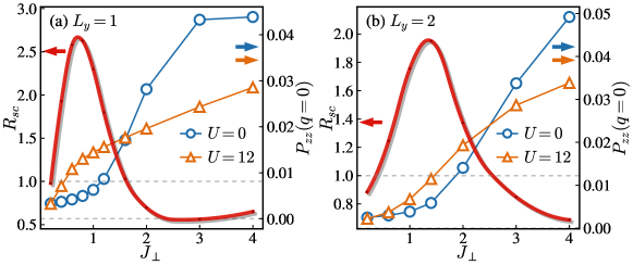
Figure CS5: The overall magnitude $P_{zz}(q=0)$ of the pair-pair correlator $P_{zz}(r)$ vs. interlayer exchange coupling $J_{\perp}$ for different on-site repulsion $U$ together with the relative ratio $R_{sc}$. The system size is $64\times 1\times 2$ for panel (a) and $32\times 2\times 2$ for panel (b), respectively.

In the following, we show some other correlators together with their relations with $J_{\perp}$ and $U$. The pair-pair correlators for singlets are defined as

$$P_{\alpha\beta}(r)=\langle\Delta_{i,\alpha}^{\dagger}\Delta_{j,\beta}\rangle,$$ (CS49)

respectively, where $|i-j|=r$ is the real-space distance between lattice site $i$ and $j$. Here we focus on the correlators along the $\hat{x}$ direction by taking $i=(x,y,\alpha)=(x,0,0)$ and $j=(x+r,0,0)$ and set the reference site at $x=L_{x}/4$. $\Delta_{i,\alpha}^{\dagger}=\frac{1}{\sqrt{2}}\sum_{\sigma}\sigma c_{i,\sigma}^{\dagger}c_{i+\alpha,-\sigma}^{\dagger}$ is the singlet pair creation operator defined at the bond between site $i$ and $i+\alpha$. $\alpha,\beta\in\{\hat{x},\hat{y},\hat{z}\}$ denote the bond orientation. The Fourier transform is $P_{\alpha\beta}(q)=\left|\sum_{r}P(r)e^{iqr}\right|/R$, the peak value of which can be regarded as the overall magnitude of the correlation. Fig. CS4 shows the typical behavior of the interlayer nearest-neighbor pair-pair correlator $P_{zz}(r)$. One can see that in spite that all of them are quasi-long-ranged, $P_{zz}(r)$ in systems with $U=12$ is larger than that with $U=0$ for both $L_{y}=1$ and $L_{y}=2$. Fig. CS5 depicts that the overall magnitude of $P_{zz}(r)$ in systems with $U=12$ is larger than that with $U=0$ around $J_{\perp}\sim t_{\|}$, as indicated by the peak of the dimensionless ratio $R_{sc}=P_{zz}(q=0,U=12)/P_{zz}(q=0,U=0)$.

We can also investigate the local pairing strength of holes through the holon-holon density correlator between interlayer nearest-neighbor sites

$$C_{h}(i)=\langle n^{h}_{i1}n^{h}_{i2}\rangle-\langle n^{h}_{i1}\rangle\langle n^{h}_{i2}\rangle,$$ (CS50)

where $n^{h}_{i\alpha}$ is the holon density at site $i$ and layer $\alpha$ defined by $n^{h}_{i\alpha}=(1-n_{i\alpha\uparrow})(1-n_{i\alpha\downarrow})$. We estimate the local pairing strength via the overall magnitude $\bar{C}_{h}$ by taking average over all sites, i.e., $\bar{C}_{h}=\sum_{i}C_{h}(i)/(L_{x}L_{y})$. As shown in Fig. CS6, $\bar{C}_{h}$ in systems with strong on-site repulsion $U=12$ is always larger than that with $U=0$, for both system widths $L_{y}=1$ and $L_{y}=2$. The relative ratio $R_{h}=\bar{C}_{h}(U=12)/\bar{C}_{h}(U=0)$ is also significantly large at $J_{\perp}\lesssim t_{\|}$. This implies that given a holon at site $i$ and layer $1$, it is more likely to find another holon at site $i$ and layer $2$ in systems with $U=12$ than those with $U=0$. This data provides additional evidences for the enhancement of interlayer pairing strength from the on-site repulsion, compensating for the deficiency that the binding energy shown in the main text mixes the contributions from interlayer and intralayer pairing.

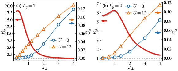
Figure CS6: The averaged interlayer nearest-neighbor holon-holon correlation $\bar{C}_{h}$ vs. interlayer exchange coupling $J_{\perp}$ for different on-site repulsion $U$ in systems of (a) $L_{y}=1$ and (b) $L_{y}=2$. The system length is fixed at $L_{x}=32$.