Statistical Aspects of X-ray Spectral Analysis

Let’s imagine that we have received an X-ray spectral file with corresponding auxiliary files (.arf and .rmf), known to come from an observation of a point source. We are told by our advisor to “fit the spectrum with a power law”. Section 1 explores what that means exactly. There are subtleties involved when inferring physically-meaningful information about a system from an X-ray spectrum, which can seem daunting to even experienced X-ray astronomers. This chapter provides a step-by-step introduction (Section 1) to performing X-ray spectral fitting in practice, and investigates the subtleties involved. Frequentist data analysis and Bayesian inference are discussed in Sections 2 and 3, respectively. Hands-on exercises are included for both. Section 4 and 5 cover more advanced concepts, such as a framework for inferring sample distributions. Further reading material for specialised and advanced topics is listed in Section 5.

To cover the essential concepts, the scope of this chapter is necessarily limited. Mathematical details on statistics can be found in the further reading section at the end (Section 5). The examples and discussion focus on the analysis of an isolated X-ray point source observed with focusing optics and a charge-coupled detector. From this case we hope the reader can apply the learned concepts to other situations. The hands-on exercises focus on two widely used X-ray spectral analysis packages, Sherpa and Xspec. However, the same analyses could be made with other packages as well.

1 The story of detected X-ray photon counts

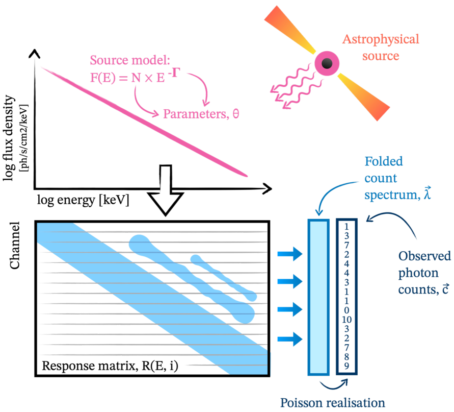
Figure 1: The X-ray measurement process and its linear approximation (eq. 1). The X-ray spectrum emitted by the astrophysical source (pink, $F(E)$) is modified by the instrument response (matrix), which encodes the energy-dependent response. The observed X-ray events are recorded in detector channels (horizontal lines). The spectral model $F(E)$ is forward folded through a response matrix $R$ to obtain a folded count spectrum $\vec{\lambda}$. The observed photon counts $\vec{c}$ are a Poisson realisation.

X-ray observations are typically based on photon counting, where each count has a reconstructed energy which is not trivially related to the original X-ray photon’s energy. As discussed in Fioretti & Bulgarelli, (2020), the process of collecting X-ray photon counts in the case of spectro-imaging detectors behind Wolter-type optics without pile-up can be linearly approximated. Then in a detector channel $i$, the expected number of detected count events is:

$$\lambda_{i} =\int_{0}^{\infty}R_{i}(E)\times F(E)\times\Delta t\,dE$$ (1)

$$\approx\sum_{j}R_{ij}\times A_{j}\times F_{j}\times\Delta t\times\Delta E_{j}$$ (2)

Here $E$ is the photon energy in keV, $\Delta t$ is the exposure time. The time-averaged spectral flux density of the source of radiation in units of erg/s/cm²/keV, $F(E)$ is represented by a vector $F_{j}$. The X-ray measurement process is shown in Figure 1.

The instrument response, $R$, can be separated into a row-wise normalised energy redistribution matrix $R_{ij}$ and a normalising area $A_{j}$, which carries the units of $\mathrm{cm}{{}^{2}}$ and describes the telescope’s sensitivity at that energy (see Figure 2). $R_{ij}$ is typically not invertible, so we cannot infer $F$ uniquely from the spectrum. Instead we need to forward-fold the measurement process to identify plausible physical spectra $F$ that match the observed data. The linear approximation is illustrated in Figure 1. Nevertheless, $R$ often has a diagonal band, which allows assigning the detector channels a nominal energy designation, which is helpful for interpretation and visualisation.

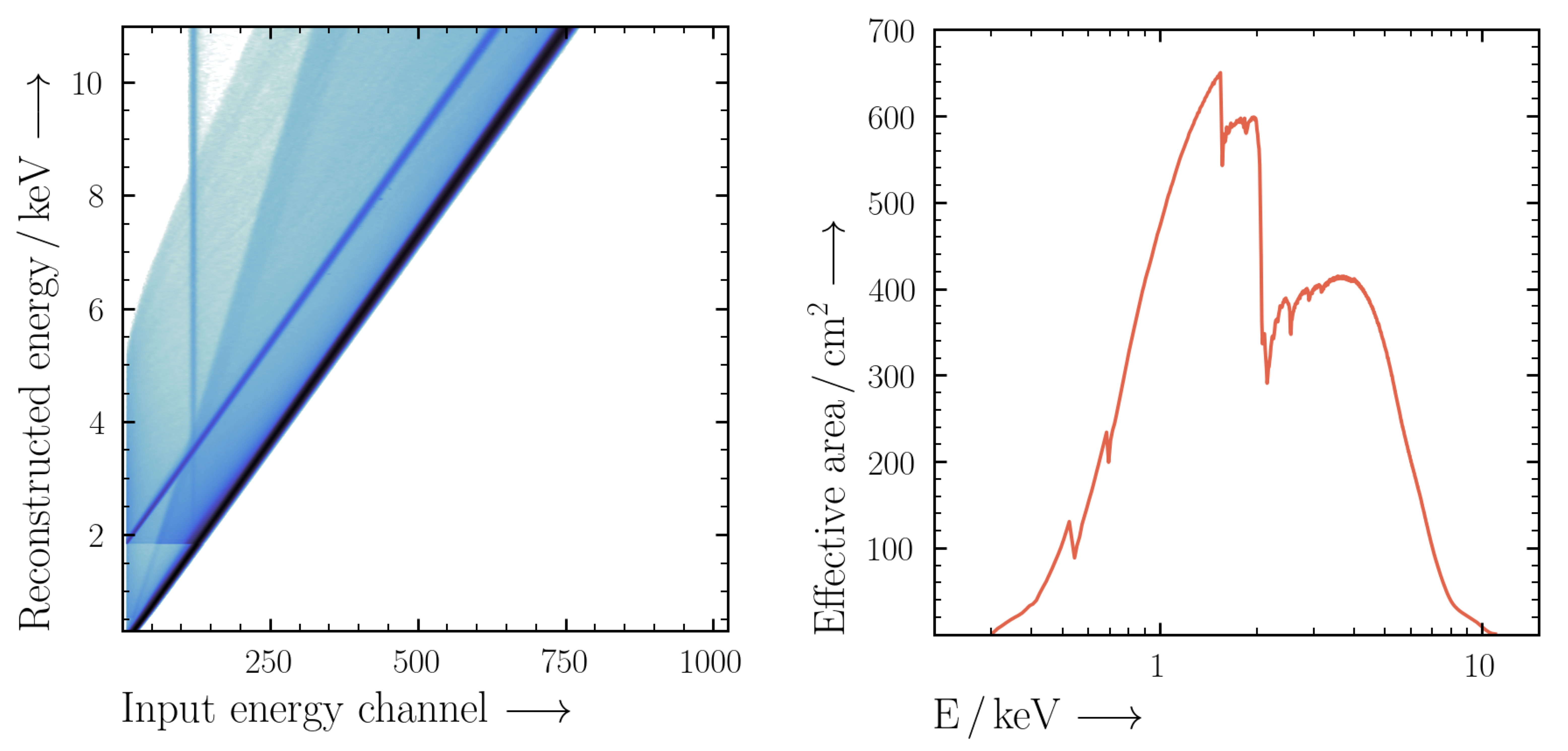
Figure 2: Response files for an X-ray spectrum. Left panel: An example energy redistribution matrix (.rmf file) for a Chandra/ACIS observation. A given energy channel detects a charge, which has a strong probability of having originated from a particular energy photon (the dark diagonal band). However, there is still a finite chance that the charge detected was excited by a photon of higher energy that triggered secondary photons. Right panel: The effective area (.arf file) for the same observation, describing the telescope’s sensitivity at particular energies. The strong absorption edges are caused by incoming photons interacting with the telescope mirrors.

Under the linear approximation, given an astrophysical source model ($F$), and an instrument model ($R$), we can predict the average number of photon counts detected, $\lambda_{i}$ in one detector energy channel. Say, for example, $\lambda_{i}=4.2$ counts are expected. Now if you look into your spectral fits file, you will see that the number of counts in each channel, $c_{i}$, is an integer number (0, 1, 2, etc), which describes how many photon events have been detected and assigned to a given energy channel. The number of counts assigned to each energy channel is therefore a stochastic realisation of the expected number $\lambda_{i}$, and can be described by a Poisson process:

$$c_{i}\sim\mathrm{Poisson}(\lambda_{i})$$ (3)

In words: $c_{i}$ is randomly sampled from a Poisson distribution with expectation $\lambda_{i}$. The Poisson probability to sample $c_{i}$ counts given an expected number of counts of $\lambda_{i}$ is (illustrated in Figure 3):

$$P_{\mathrm{Poisson}}(c_{i},\lambda_{i})=\frac{\lambda_{i}^{c_{i}}\times e^{-\lambda_{i}}}{c_{i}!}$$ (4)

The likelihood describes how frequently, under the assumed model $\lambda(R,F,...)$, we expect to see $c_{i}$ counts. This bears repeating: it describes the tendency of a given model to produce $c_{i}$ counts.

Figure 3: The Poisson and Gaussian probability distributions. There are six key differences: Poisson is defined over (1) non-negative (2) integer values, while the Gauss can be negative and is continuous. (3) The Gauss distribution is symmetric, while the Poisson is asymmetric. (4) At the low value end the Poisson distribution is steeper than the Gauss, while (5) at the high end, the Poisson is shallower than the Gauss. (6) The Gauss distribution has two parameters (mean and standard deviation), while the Poisson has one (expected number of counts).

This is convenient since we can now try to search for models which have a high probability of producing the data (i.e. counts) that we observe! But first there are a few things to tighten up.

1.1 Combining independent data

Since we have data in multiple energy channels (it is a spectrum, after all), we want to use them. Since the probabilities are independent, the probability of all data is the product of the individual ones:

$${\cal L}(\theta)=P(\overrightarrow{c},\overrightarrow{\lambda}(\theta))=\prod_{i}P(c_{i},\lambda_{i}(\theta))$$ (5)

Given the prediction $\lambda_{i}$ in each channel, which depends on the model parameters $\theta$, this likelihood ${\cal L}(\theta)$ gives us the probability over all data counts considered.

Eq. 5 also applies for simultaneously analysing multiple data sets. For example, when combining data from a low-energy instrument such as eROSITA with a high-energy instrument such as NuSTAR. In each considered detector channel the predictions are compared to the observed counts and the probabilities multiplied following eq. 5.

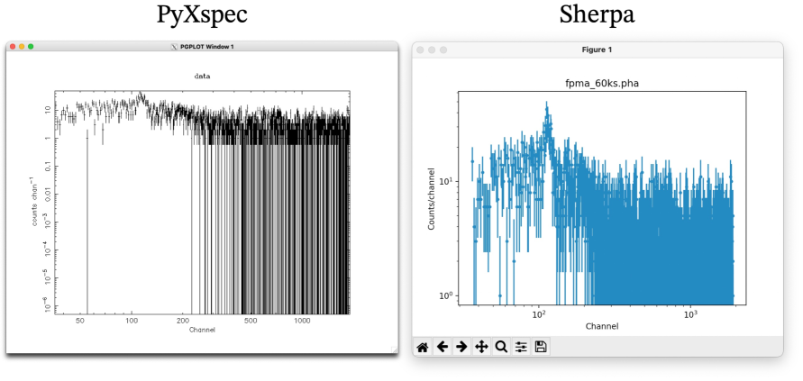
Figure 4: Detected channel vs. number of counts for Exercise 1 with PyXspec (left) and Sherpa (right). The error bars with long tails to the bottom are those with one count, where the error is estimated to be also 1, thus reaching down to zero. Data points corresponding to zero counts are missing altogether in this visualisation.

1.2 Understanding chi² and CStat

Now we have the machinery set up to calculate the probability of the process to make the observed data, given a source flux model and its parameters $\theta$. The natural next step is to try to find the model parameters that maximize this probability. It has become convention in computer science to build machinery that minimizes (cost) functions, which can be adopted by flipping the sign of a function to maximize. For numerical accuracy it is convenient to work in logarithms. Taken together, it has become standard practice to minimize the fit statistic $-2\times\log P(\theta)$.

For the Poisson likelihood (eq. 4), and dropping constants, we obtain the statistic:

$$\mathrm{``CStat"}=\sum_{i}c_{i}\log\lambda_{i}-\lambda_{i}$$ (6)

If one obtained instead channel data drawn from a Gaussian process,

$$d_{i}\sim\mathrm{Normal}(\lambda_{i},\sigma_{i})$$ (7)

then the likelihood is

$$P_{\mathrm{Normal}}(d_{i},\lambda_{i})=\frac{1}{\sqrt{2\pi}\sigma}\exp\left\{-\frac{1}{2}\left(\frac{d_{i}-\lambda_{i}}{\sigma}\right)^{2}\right\}$$ (8)

and the minimization statistic, following again $-2\times\log P(\theta)$, becomes:

$$``\chi^{2}"=\sum_{i}\left(\frac{d_{i}-\lambda_{i}}{\sigma_{i}}\right)^{2}$$ (9)

Here we see where the multiplication of two came from. It makes the form for the Gaussian case most convenient. The correspondence of $\chi^{2}$ and Gaussian probability density is illustrated in Figure 5.

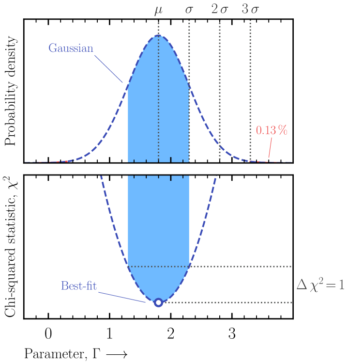
Figure 5: Relation between Gaussian distribution and fit statistic ‘$\chi^{2}$’. The Gaussian distribution has mean $\mu$ and standard deviation $\sigma$, whereas ‘$\chi^{2}$’ is twice the negative logarithm. The area within 1 sigma ($\Delta\chi^{2}<1$) and beyond $3\sigma$ is illustrated.

Thus saying “I use chi² statistics” is a short-hand for “I assume a Gaussian measurement model”, while “I use CStat” is shorthand for “I assume a Poisson count process”. The former has an additional uncertainty parameter for each channel, $\sigma_{i}$.

When should one employ C-Stat and at what point is $\chi^{2}$, with some $\sigma_{i}$, an appropriate approximation? The $\chi^{2}$ statistic leads to biased model parameter estimates, as illustrated in Figure 6. Poisson data were simulated from a powerlaw model $A\times i^{-\Gamma}$ where i is the channel index from 0 to 100, $A$ is the powerlaw amplitude and $\Gamma=1$ is the powerlaw index. Then, the model parameters were fit for by optimization. $\chi^{2}$ statistics are biased by over 5 per cent when using fewer than $\sim$40 counts, with the amplitude under- and the index over-estimated. This bias decreases towards higher counts. However, a systematic offset remains that is comparable to the statistical uncertainties and thus has a statistically significant impact at all counts (Humphrey et al.,, 2009).

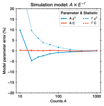
Figure 6: A $\chi^{2}$-based fit (blue curves) of a power-law under-estimate the amplitude (solid curve) and over-estimate the powerlaw index (dotted curve). C-stat (green) is unbiased. Based on Mighell, (1999).

In contrast, C-Stat is unbiased at all counts (Cash,, 1979). Figure 6 also shows that switching from C-Stat to $\chi^{2}$ when the spectrum has at least 30 counts causes a 5 per cent discontinuity in the estimated model parameters. Historically, faster computation time favoured $\chi^{2}$, however, today, computation is dominated by source models rather than the statistic. Fast computers and modern inference algorithms mean C-Stat can be used at all levels of count statistics. More information can be found in Wheaton et al., (1995); Nousek & Shue, (1989); Mighell, (1999) and the introduction of van Dyk et al., (2001).

1.3 Detector details, binning and grouping

When an X-ray hits a charge-coupled detector, an electron charge is deposited onto one or more pixels. These are then grouped into an event, and the electron charge estimated (see Fioretti & Bulgarelli, 2020 for more details). The charge is converted into an energy channel, on a binning that makes sense for the given instrument. The binning can sometimes be chosen by the user of the analysis pipeline, or modified after.

The binning is often rather fine, to not hinder any scientific investigations. However, the detector response sets some fundamental limits on how much information, even with high numbers of counts, can be extracted. Kaastra & Bleeker, (2016) proposed optimal binning of the spectrum based on the detector response. This typically reduces the computation time in parameter estimation, with essentially no loss of information. We recommend this procedure, which is implemented in ftgrouppha (included with HEASARC’s ftools; see exercise 3). While this re-binning method can be considered a good starting point, some fit statistics may require further, coarser re-binning to reach a minimal number of counts.

A further motivation to apply coarser binning is that the detector response is not perfectly describing the instrument behaviour. For example, detector edges or peaks may not be positioned perfectly. Such systematics can bias the spectral fit.

To reach the regime where $\chi^{2}$-based estimates are approximately valid (see Figure 6), further grouping of the detector channels can be applied as a data pre-processing step. Strategies include binning n-fold, adaptively by signal-to-noise ratio or minimum number of counts, by tools such as ftgrouppha and Sherpa. Broad energy bands (e.g., 0.5-2 keV, 2-10 keV, 15-195 keV) are an extreme case. In the process of such rebinning, spectral shape information is always lost. How much information is lost depends on the spectral model. In case of smooth continuum models, the impact may be less severe than for identifying narrow lines. Rebinning is unnecessary when Poisson statistics are used. Bins with zero counts are fine. However, see the next section for how handling background spectra change the situation.

In addition to the requirements for fitting, it can be difficult to visualise the shape of the observed spectrum without some level of binning. Therefore, separately from the statistical analysis, it is useful to rebin the data for visualisation purposes. Within Xspec, the setplot rebin command (Plot.setRebin() in PyXspec), combines adjacent bins to have some minimum significance, which can make it easier to interpret the shape of the data being fit. This command has no effect on the fitting.

1.4 Background spectra

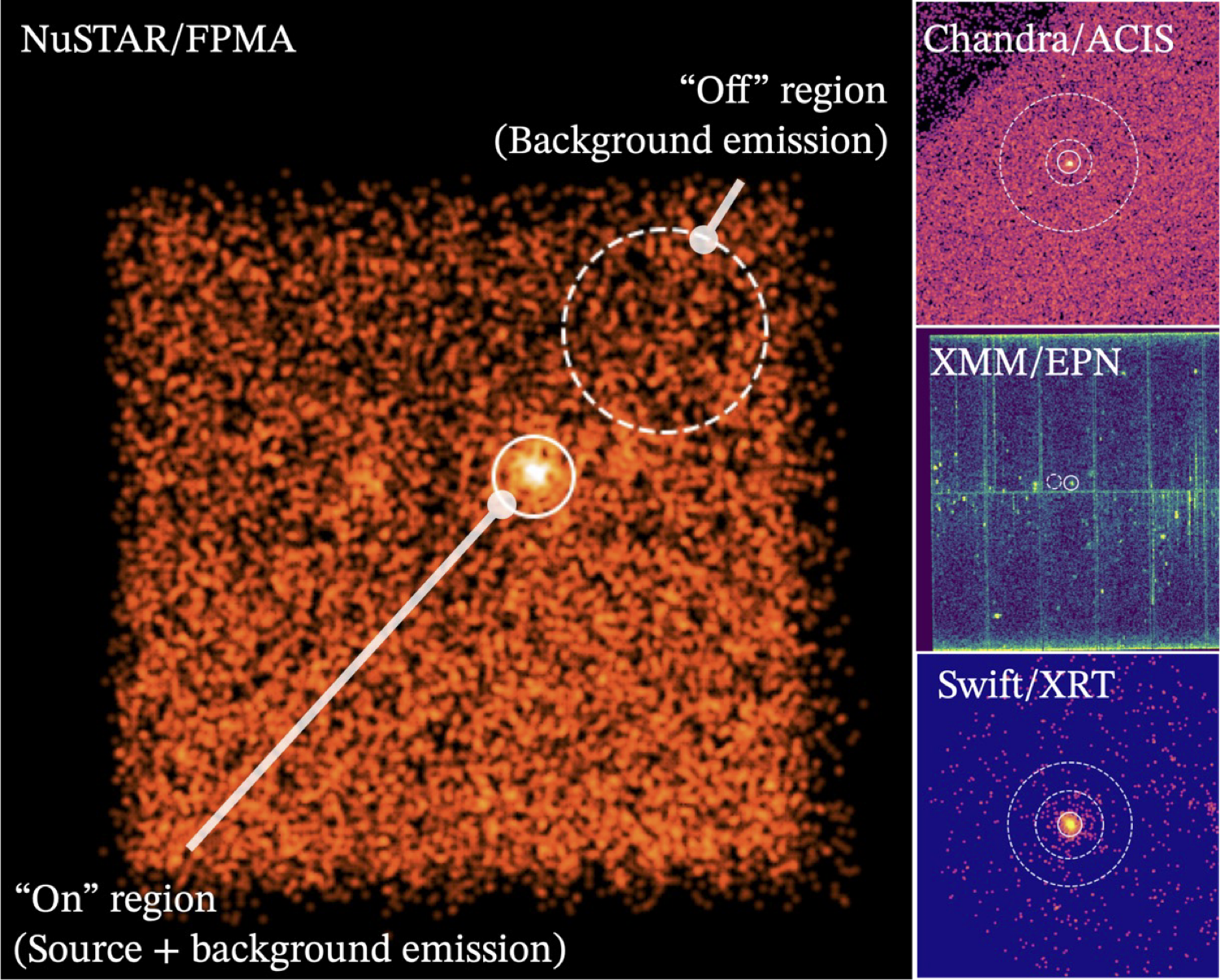
Figure 7: On and off region treatment. In the typically larger off/background region (dashed lines in each panel), only the background processes are assumed to contribute. In the on/source region (solid lines), both the background and source emission contribute. Examples are shown for NuSTAR/FPMA, Chandra/ACIS, XMM-Newton/EPN and Swift/XRT.

A special case of the combination of data is when one spectrum was taken in an “off” time or “background region”, where only background radiation processes are assumed to contribute, and another spectrum was taken in an “on” time or “source region”, where both the background and the source process of interest contribute. This is illustrated in Figure 7.

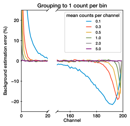
Figure 8: When binning the background to at least one count per group, the background level in the first (last) channels tend to be systematically over- (under-)estimated. This is caused by the rebinning adaptively changing the bin edges starting from the lowest filled channel and ending at the high end, which causes fluctuations of the bin edges and widths.

To use eq. 5 in this case, we have for the on region $\lambda_{i}^{\mathrm{on}}=\lambda_{\mathrm{src},i}+\lambda_{\mathrm{bkg},i}$ and for the off/background region $\lambda_{i}^{\mathrm{off}}=\lambda_{\mathrm{bkg},i}$. In the process of computing $\lambda$ from the flux, different areas and exposure times for the on and off regions may need to be considered.

In some cases, the background contribution to the observed counts is much smaller than the source contribution at all considered energy channels, and it can be ignored. Otherwise, a model for the background needs to be defined. These can be either non-parametric or parametric, and informed from other observations or solely based on the observation at hand.

Figure 9: Chandra example background spectrum. The spectrum is divided by exposure time and bin energy width. Still, the Poisson nature (non-negative integer values) is clearly visible. Two empirical background models of different complexity consisting of continuum and line shapes are plotted in blue and red. Taken from Buchner et al., (2014).

Figure 9 shows an example of an auxiliary background model fitted to a Chandra background. The model is an empirical mixture of power laws and Gaussians, without attempting to assign physical meaning to the components. For other examples of background modelling, see Wik et al., (2014) (physical model for NuSTAR) and Maggi et al., (2014) (semi-physical model for XMM-Newton). Defining such models can have the benefit of (1) propagating the background uncertainties and (2) taking into consideration that the background may not vary rapidly between detector channels. The latter is reasonable when there are no strong response edges or in the case of the cosmic particle background. Parametric background models can also be machine-learned by analysing large sets of archival observations (see Appendix of Simmonds et al.,, 2018), which do not necessitate physical knowledge of the background itself.

Sometimes we are not able to build a detailed model for the background. In that case, we could try to estimate the background contribution in each detector channel directly. A naive estimate with the channel counts of the background region would be $\lambda_{\mathrm{bkg,i}}^{\mathrm{off}}\approx b_{i}$. A less biased estimate can be obtained by maximum likelihood. Then we can add $\lambda_{\mathrm{bkg,i}}$ to the source count prediction. Taking into consideration differences in region definition, that is:

$$\lambda_{i}^{\mathrm{on}}=\lambda_{\mathrm{src},i}+\lambda_{\mathrm{bkg,i}}^{\mathrm{off}}\times\frac{A_{\mathrm{on}}}{A_{\mathrm{off}}}\times\frac{\Delta t_{\mathrm{on}}}{\Delta t_{\mathrm{off}}}$$ (10)

This profile likelihood (meaning the optimum for the nuisance parameter was determined) approach is called the WStat statistic (Wachter et al.,, 1979), and is a modification of CStat (Cash,, 1979). Instead of subtracting the background, which would not depart from Poisson statistics (Skellam statistics), WStat adds a background contribution to the source model in each channel.

Fitting with WStat has two complications: firstly, the uncertainty by not knowing $\lambda_{\mathrm{bkg,i}}^{\mathrm{off}}$ precisely is not propagated into the source flux estimate. Secondly, biases in the predicted source counts can occur if the background is not sampled with a sufficient number of counts, in a sufficient fraction of the background bins.

In such cases, some bins will have zero counts, the background will be underestimated and the source flux will be over-estimated. These issue are explored in a numerical study by Giacomo Vianello.

One way to rectify this problem is to adaptively bin the source spectrum such that the background spectrum bins contain a minimum number of counts. In general, data-dependent rebinning, and then estimating something from the same data, should be treated with caution. Indeed, rebinning to a minimum of 1 count per bin is often biased, as illustrated in Figure 8. The numerical study⁵ shows that grouping to a minimum of 5 bins seems to give an acceptably low bias. The grouping needs to be based on the counts in the background spectrum. The grouping needs to be stored in the source spectrum (see exercise 3), because the source spectrum binning determines how the background spectrum is treated, in e.g., Xspec. The discussed issues are relevant for WStat statistics, which is used by default in Xspec when the statistic is set to ”cstat” and a background is loaded.

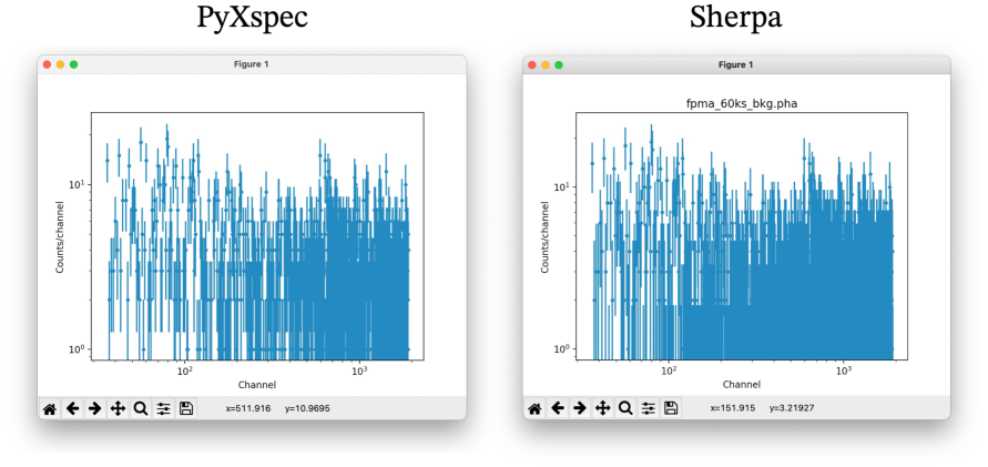
Figure 10: Detector channel vs. number of background counts for Exercise 2 with PyXspec (left) and Sherpa (right).

2 Frequentist data analysis

2.1 Fitting by minimization

Now we can stick these statistics into some off-the-shelf minimizer. These are general-purpose computer algorithms that begin from a user-provided parameter guess, and iteratively walk around the parameter space in such a way to minimize this “cost” function. Many minimizers exist, the most common in X-ray spectral fitting being the Levenberg-Marquardt algorithm, the Nelder-Mead simplex method and differential evolution. Of these, Levenberg-Marquardt considers the model gradient (which is however typically not available) to guess the next point assuming a locally quadratic landscape. The assumption is optimal for the case of $\chi^{2}$ (note eq. 9 is a quadratic polynomial), but not CStat. The simplex method evolves a group of points, always replacing the worst fit with a new linear combination of the remaining points, to wander towards the minimum, and is quite robust.

In complicated models, there may be multiple but distinct regions of the parameter space which provide comparable fit quality. Which of these local optima is found by the minimizer is partially determined by the initial guess and partially random. The properties above lead to the unsatisfying activity of repeatedly restarting the minimizer to another starting point, or strategies of scanning over one parameter while optimizing the remainder to escape such local optima and discover the global minimum in fit statistic. Fancier algorithms such as differential evolution try to mitigate this problem by maintaining a large population of points that searches the parameter space.

Whichever minimizing algorithm is employed, the algorithm iterates until a stopping criterion is reached. This is typically an estimate that any further refinements in the best-fit parameters only lead to improvements smaller than a threshold $\epsilon$.

At the end of the minimization process, we have the parameters $\hat{\theta}$ which most frequently produce the observed data. For example, if we fit a power law model $F=N\times(E/1\,\mathrm{keV})^{-\Gamma}\mathrm{erg/s/cm^{2}/keV}$ with two parameters, $\theta=(N,\Gamma)$, the minimizer may gleefully report: $\Gamma=1.26$! As physicists, this is not the end of our analysis because the next, and often more important, question is: which $\Gamma$ values are ruled out by the data?

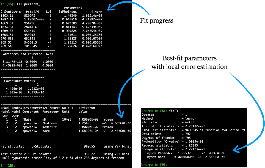
Figure 11: iPython output in PyXspec (left) and Sherpa (right) from the commands given in Exercise 4. A number of useful quantities are given in both, including the fit statistic value, number of degrees of freedom and corresponding parameter values. From the optimizer’s limited exploration, also a rough uncertainty estimate around the (locally) best fit is given.

2.2 Frequentist error analysis

To estimate uncertainties on our model parameters, let’s assume a few things are true. First, let’s assume the model is linear in its parameters. Secondly, let’s assume we are always far from boundaries of the parameter space. Thirdly, let’s assume we are in the high-data regime, i.e., that every spectral bin has many counts and all model parameters can be constrained well. In that (optimistic) case, considered by Wilks’ theorem (Wilks,, 1938), one can make a second-order Taylor expansion of the statistic, in other words, it falls off quadratically. This is akin to a Gaussian distribution. With this picture in mind, it makes sense to ask what the $1\sigma$-equivalent parameter range is. This can be estimated by the quadratic approximation that the minimizer already built internally and reports as errors (see Figure 11).

However, in many realistic cases, none of the three assumptions are fulfilled in X-ray astronomy. The approximation can be poor, most frequently producing under-estimated errors, for example because of non-linear degeneracies. Instead, it is common to scan the parameter space by varying each parameter in turn, while simultaneously optimizing the other parameters. This is called ”profiling the likelihood” and illustrated in Figure 5. Where the statistic has worsened by $\Delta=1$, the $1\sigma$ equivalent is reached, and this defines the $1\sigma$ confidence intervals. Equivalently $\Delta=2$ for $2\sigma$-equivalent confidence intervals.

Now, what precisely are confidence intervals supposed to describe and do they? If we assume that the optimal parameters obtained, $\hat{\theta}$, are the true parameters of the process out there in the Universe, and we generate many thousands of spectra that could have been observed, and for each of them the minimum was determined and a $1\sigma$ confidence interval constructed as described above, then the true value $\hat{\theta}$ is contained in $68\%$ of these confidence intervals. This is the definition of confidence intervals.

Since in many cases either the model is not linear, or we are not in the high-data regime or we are not away from the parameter boundaries, or we do not necessarily trust our minimizer to be perfect, this is not quite right. Therefore, we have to actually simulate a thousand spectra, fit them, and look how the confidence intervals actually behave. We could calibrate $\Delta$ so that the constructed confidence intervals contain the input value $68\%$ of the time. Then, we have the desired property without needing strong assumptions. This is a typical activity for observing proposals, where we want to convince a panel that with the obtained spectrum, no matter the random realisations, we can constrain some parameter of interest with high probability.

2.3 Model checking

We perform the above exercise and find $\Gamma=1.26\pm 0.1$. Beautiful! Then our advisor asks us to make a plot of the spectrum and the model fit. So we plot the observed counts $d_{i}$ against the model predicted counts $\lambda_{i}$. Our heart sinks: these look nothing alike! Our $\Gamma$ constraint is not meaningful.

This process is formalised in model checking, which tests whether the model could produce the observed data. Importantly, the model is considered in isolation, without alternatives.

The first approach is to consider a null hypothesis significance test, where either the model defined is true, or another (unspecified) model is true. We consider the data that could have been stochastically produced by our model, and look whether the data the telescope actually recorded are an implausibly infrequent outlier. We could generate thousands of Poisson counts from the model, and count what fraction of these realisations lie above the observed counts $c_{i}$, which is the p-value. In the case of a Poisson distribution, this can also be computed analytically:

$$p=\sum_{c_{i}^{\prime}=c_{i}}^{\infty}P_{\mathrm{Poisson}}(c_{i}^{\prime},\lambda_{i})$$ (11)

With the conversion between p-value and $\sigma$ from the Gaussian distribution (a common convention), we would call it a $3\sigma$ outlier if $p=0.1\%$. However, if the channel bins are fine, each bin may have little information to judge a model in this way. To address this, we could rebin channels together for this test (see rebinning above). One may be tempted to consider the cumulative count distribution, $C_{i}=\sum_{j=1}^{i}c_{j}$, with a Kolmogorov-Smirnov or Anderson-Darling test. However, since we determined $\hat{\theta}$ from the same data $c_{i}$ by optimization, its p-values are not valid (see https://asaip.psu.edu/Articles/beware-the-kolmogorov-smirnov-test/). Kaastra, (2017) analysed how the CStat may be used directly as a measure of the goodness of fit.

The second approach is to visualise the data and think about it. You can try various visualisations, such as grouping channels together to get a clearer impression of the deviations, residual plots, cumulative plots of $C_{i}$, etc. This will give you ideas of what could be wrong, and suggest alternative models to try. How to compare among multiple plausible models is explained below. Visualisations (and thinking) are highly recommended approaches. Not everything has to be a test.

For further reading on model checking and detection of components via reduced chi square, F-test and likelihood ratio tests, and their pitfalls, we refer the reader to Protassov et al., (2002); Andrae et al., (2010).

Figure 12: ‘Q – Q difference’ plot for the frequentist Levenberg-Marquardt fit of model1 from Exercise 6. Plotted on the y-axis is the difference between the cumulative ‘data’ counts (i.e. the cumulative source $+$ background counts) and the cumulative model (including the background) counts. The clearest feature in the plot is a large deficit of counts $\lesssim$ 6 keV. The cumulative has been normalised to unity. Cumulative-based plots have the benefit of not being dependent on binning for visual clarity, apart from the binning required for the fit itself.

2.4 Model comparison

Finally, we can consider the situation where two models of physical processes of equal a-priori plausibility are to be judged by the data. Is model A significantly better than model B? This is also a case of null hypothesis significance testing, if model A is the null hypothesis, and we want to reject model A in favour of the alternative hypothesis B. This has two possible outcomes: either the rejection is successful, in which case model B is picked because there was enough evidence for model B. Or the rejection is unsuccessful, in which case model A is kept, either because it is better or because there was not enough distinguishing evidence. Again, the null hypothesis significance test needs a confidence threshold, e.g., $p<1\%$. This sets how often we would erroneously prefer model B over model A even when model A was true (false positive rate, or type I error, see Table 1 and Figure 13).

In contrast, the false negative rate (type II error) is the erroneous preference of model A when model B was true. Ideally, one would like both errors to be small, but this depends on the model test (see Figure 14).

Output $\rightarrow$	Model A found	Model B found
True input $\downarrow$	(negative)	(positive)
Simpler model A (null)	true negative	false positive (type I error, $\alpha$)
Complex model B (alternative)	false negative (type II error, $\beta$)	true positive (power)

Table 1: Confusion matrix. Even if the simpler model A were always true (first row), the decision procedure under a certain threshold may falsely claim a detection of model B, giving a false positive. Alternatively, even if model B is actually true (second row), the data may not provide enough evidence to the decision procedure to prefer model B over model A, giving a false negative. These concepts apply to any method for making decisions, but have different names in different disciplines. The terms used by statisticians are in blue.

In the idealised situation considered above (linear model, high-data regime, away from the parameter bounds), which does not hold in X-ray astronomy, there are analytic statistical tests which consider the statistic difference ($\Delta\mathrm{CStat}=\mathrm{CStat}_{A}-\mathrm{CStat}_{B}$ or $\chi_{A}^{2}-\chi_{B}^{2}$) between the two models. These include the F-test and likelihood ratio test. Do not use these. Do not trust the results of these, because their assumptions are not valid for our data.

You can however build a reliable null hypothesis test from what we have already discussed: simulate 1,000 spectra from the null model (model A), fit each with both models, and compute the statistic difference $\Delta\mathrm{CStat}$. This gives you a distribution of $\Delta\mathrm{CStat}$ values expected if the null model was true. In rare cases, by chance, model B may be more prone to produce the observed data, $\Delta\mathrm{CStat}>0$. Reading off the $99\%$ quantile, we obtain a $\Delta\mathrm{CStat}$ threshold $\Delta\mathrm{CStat}_{\mathrm{crit}}$, which sets the type I error to $1\%$. This is a subtle point, but follows from the definitions: we have simulated under model A, and in 1% of cases this $\Delta\mathrm{CStat}_{\mathrm{crit}}$ is exceeded. In other words, if we apply our calibrated criterion $\Delta\mathrm{CStat}>\Delta\mathrm{CStat}_{\mathrm{crit}}$, and select model B, the purity of this process is 99%.

To obtain the power of our test to distinguish the models (1 - false negative rate), we would have to simulate under model B, and count the fraction of cases where we indeed select model B.

Figure 13: False positive (type I) error. Following Exercise 8.1 (and Table 1) to estimate the false positive (i.e. type I) error, we simulate from the simpler model 1 and re-fit with both model 1 and model 2. Here we plot the resulting distribution of $\Delta W_{n}$ = $W_{\rm model\,2}\,/\,n_{\rm model\,2}$ – $W_{\rm model\,1}\,/\,n_{\rm model\,1}$ from the simulations. The 99th quantile from the distribution is a value of 0.02 – thus if we choose this value of $\Delta W_{n}$ for our threshold, we would expect to select the more complex model 2 $\sim$ 1% of the time in the event that the null model 1 was correct.

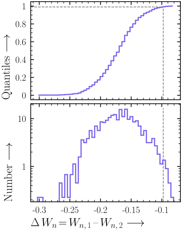
Figure 14: False-negative (type II) error. In contrast to Exercise 8.1, we now simulate from the more complex model 2 before re-fitting with both model 1 and model 2. Following the same prescription as in Figure 13, we plot the resulting distribution of $\Delta W_{n}$, and find the 99th quantile to be 0.098. Thus if we choose this to be our threshold, we would expect to preferentially select model 1 $\sim$ 1% of the time, when the more complex model 2 was correct. We can also say that at this $\Delta W_{n}$ threshold, the power is 99%.

2.5 Limitations so far

As you have seen above, analytic derivations make unreasonable approximations. By generating many simulated spectra and analysing them, it is however possible to get answers and be confident in our inference for excluding parameter values, and distinguishing models.

The frequentist approach describes the reliability of procedures to recover input values. In the process however, the best-fit value $\hat{\theta}$ was assumed to be the true value. What we would rather have, indeed, is a procedure which tells us what the true value out there in the Universe is, or at least a probability distribution over the true value. For example, we would like to make statements – starkly different to those possible with confidence intervals (re-read above) – such as:

• the true value of $\Gamma$ lies between 2.1 and 2.2 with 99% probability

• the true value of $\Gamma$ lies above 2.5 with 0.1% probability.

In other words, we are making statements of the integrated probability over some interval of a parameter, $\int_{a}^{b}P(\theta)\,d\theta$. By the way, when you set $a=b$ the integral becomes zero, because the probability to have exactly that value is infinitesimally small compared to all possible values; but we can live with that.

Probability distribution functions (PDFs) allow interesting ways to judge parameter ranges relative to each other. Unfortunately, there is no inference procedure that just produce these. The key reason is that to define $\int P(\theta)\,d\theta$ we assumed that we are integrating with equal weight over $\theta$. If we changed our definition of our power law model to be $N\times E^{-\log\gamma}$ instead of $N\times E^{-\Gamma}$, we would obtain the same optimal parameter $\log\gamma=\Gamma$, but $\int P(\Gamma)\,d\Gamma\neq\int P(\gamma)\,d\gamma=\int P(\Gamma)\,d\log\Gamma$.

Therefore, we need one more assumption to define probability distributions. Namely, we need to specify how “large” a region of the parameter space is relative to another region. This is known as the integration measure. In the context of the following it is also called a prior (ooooohhhh scary!). Beware if someone tells you they can, without assuming a prior make PDFs or statements like the above. There are assumptions hidden that define their prior, and they are unaware of what their inference procedure is actually doing.

Now we can introduce the mathematics of producing PDFs, namely Bayesian inference. Further below, we will combine the strengths of frequentist and Bayesian paradigms.

3 Bayesian inference

3.1 Terminology

Bayes’ theorem uses the likelihood function to update an auxiliary probability density, the prior PDF $P(\theta)$, to obtain a posterior PDF $P(\theta|D)$:

$$P(\theta|D)=\frac{P(D|\theta)P(\theta)}{P(D)}$$ (12)

This is a reordering of the terms in the law of conditional probability, with specific meanings assigned. The first term in the numerator is the likelihood, which specifies the frequency of producing a data set $D$ given assumed parameters $\theta$, ${\cal L}(\theta)=P(D|\theta)$ (specifically interpreted as ‘the probability of D given $\theta$’). The second term is the prior. Let’s call it $\pi$, so that not everything is called $P$, then we have:

$$P(\theta|D)=\frac{{\cal L}(\theta)\times\pi(\theta)}{Z}$$ (13)

The denominator normalises the posterior, $Z=\int{\cal L}(\theta)\times\pi(\theta)d\theta$, and is known as the Bayesian evidence. It is also known as the marginal likelihood, because the process of integrating away a variable $P(a)=\int P(a,b)\,da$ is called marginalisation.

3.2 Parameter estimation

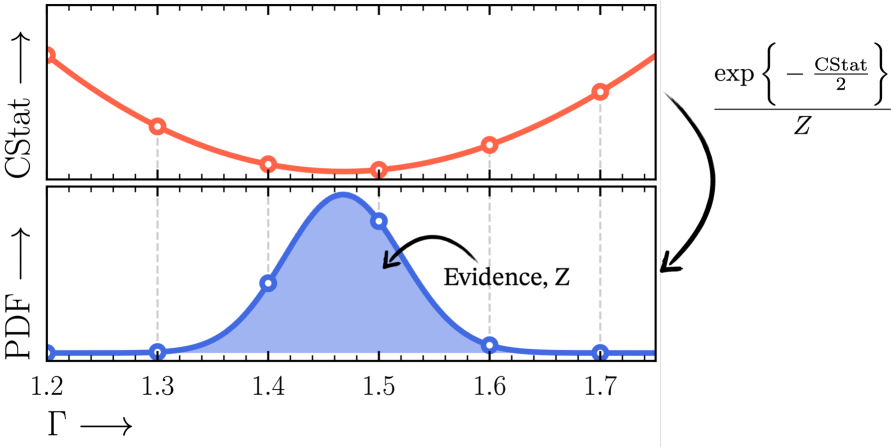
Figure 15: Bayesian inference on a grid. Stepping through the model parameter $\Gamma$, we obtain a CStat value at each grid point (red curve in the upper panel). Converting CStat to a probability ($\exp\left\{-\mathrm{CStat}/2\right\}/Z$) and normalising gives the posterior probability distribution (blue curve in the lower panel). The normalising constant is the Bayesian evidence, $Z$.

So if we make a grid in $\Gamma$, compute ${\cal L}(\Gamma)\times\pi(\Gamma)$ at each grid point and numerically integrate it, are we doing Bayesian parameter estimation? Yes. Almost everything else is numerical details. As shown in Figure 15, from a grid we can compute $Z$ with numerical integration, and then we can identify the grid intervals that contain 99% of the probability, or ask how much probability is above $\Gamma>2.5$. If we also had the normalisation as a second parameter, we would first marginalise it away and get the marginal posterior distribution of the $\Gamma$ parameter:

$$P(\Gamma|D)=\frac{\int\pi(\Gamma)\pi(N){\cal L}(\Gamma,N)\,dN}{\int\pi(\Gamma)\pi(N){\cal L}(\Gamma,N)\,dN\,d\Gamma}$$ (14)

3.3 Choosing priors

Specifying priors is a well-studied problem, and there are several approaches which can also be combined. One approach is to pick an informative prior from previous knowledge, for example from simulations, plausibility arguments or from previous studies. For example, we know today from surveys of Active Galactic Nuclei (AGN) in the local Universe, that the photon index describing the approximate intrinsic shape of the X-ray coronal spectrum is $\sim$1.8–2 with some scatter (e.g., Ricci et al., 2017). Thus a reasonable prior for X-ray spectral fitting of an AGN intrinsic (i.e. absorption-corrected) spectrum could be Gaussian distributed with mean 2 and 0.2 standard deviation.

Another approach is to define uninformative priors. Here, one considers all possible outcomes one can conceive before the experiment, and assigns them probabilities based on the principle of least surprise, the principle of maximum entropy, or such that rescaling does not change under reparameterization of the model. Skipping many technical details here, two special cases are common, which derive uniform priors in linear (for parameters with unknown offset, such as the location of an unknown Gaussian emission line) or logarithmic coordinates (such as the same Gaussian line’s dispersion and normalisation, or more generally other parameters of unknown scale).

It is good practice to try several priors that the author or readers may consider reasonable and test how sensitive the results of the study are to the assumption. In general, the posterior PDF depends on the prior, but in some situations it really does not. This is the case when the likelihood function is highly concentrated and forces the probability to go there. In this case, we say that the data are highly informative. Then, trying different priors gives the same result, as long as the prior has support where needed, i.e., the probability is not zero. How informative the data is is formalised with the ‘information gain’ or Kullback-Leibler divergence. It estimates how much the posterior changed (usually shrunk) compared to the prior distribution, typically measured in bits. For details and how to interpret the resulting numbers, see Buchner, 2022a and Figure 16.

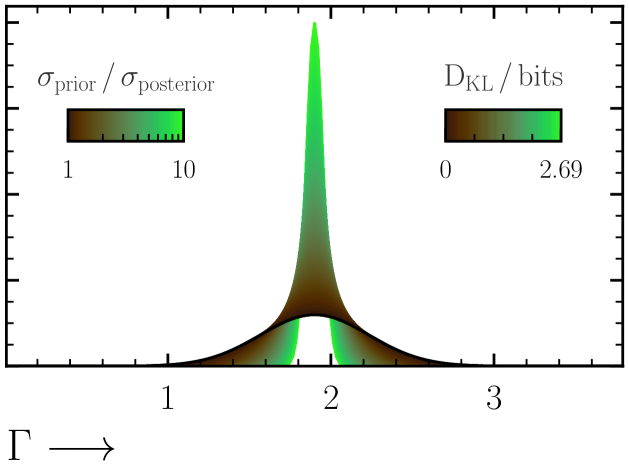
Figure 16: Measuring information gain with the Kullback-Leibler divergence. A Gaussian prior on some parameter, $\Gamma$ is assumed with fixed width, and the information gain is calculated for a series of posteriors with narrower widths than the original prior. For reference, 1 bit of information gain corresponds to a Gaussian shrinking its standard deviation by a factor of three (Buchner, 2022a, ).

3.4 Computation in multiple dimensions

With the necessary concepts of Bayesian inference, probability peaks in parameter spaces and information gain introduced, we now discuss computational issues that occur when models have many parameters. The number of model parameters, $d$, is the dimensionality of the space over which the PDF and its integration is defined. With increased parameter dimensions, uniform grids become exponentially costly to evaluate. The exponential behaviour arising from testing all parameter combinations is known as the curse of dimensionality. Smarter algorithms are needed. The most common of these is Markov Chain Monte Carlo (MCMC), and more recently Nested Sampling Monte Carlo. Here “Monte Carlo” refers to the use of random numbers to compute results. Both techniques estimate the posterior distribution, and produce several thousands of equally probable posterior samples, $\theta_{1},\theta_{2},...,\theta_{i}$, which can then be used by summation to perform the integrals mentioned above. Nested sampling additionally computes $Z$, which is useful for Bayesian model comparison (see Section 3.4.2).

3.4.1 Markov Chain Monte Carlo

Let’s first consider MCMC. We begin with a starting point $\theta_{i}$ with $i=1$, and an auxiliary proposal function, for example a narrow Gaussian distribution centred at our starting point. We draw a proposed point $\theta_{i}^{\prime}$ from the proposal function, and compare the posterior ratio of the two: $\alpha=\frac{{\cal L}(\theta^{\prime})\times\pi(\theta^{\prime})}{{\cal L}(\theta)\times\pi(\theta)}$ (Metropolis et al.,, 1953). If the posterior is higher at the proposed point $\theta^{\prime}$, i.e., $\alpha>1$, we set $\theta_{i+1}=\theta^{\prime}_{i}$. If it is lower, we still jump there $\theta_{i+1}=\theta^{\prime}_{i}$ with probability $\alpha$, and otherwise remain at the current point $\theta_{i+1}=\theta_{i}$. This Metropolis procedure creates a chain of points $\theta_{i}$ whose distribution converges, given infinite iterations, to the (unknown) posterior distribution.

Since computing time is finite, convergence is not guaranteed. There are several diagnostics that can be used to test whether a limited chain or several chains are problematic. Here we recommend in particular the $\hat{R}$ diagnostic (Gelman & Rubin,, 1992; Vehtari et al.,, 2019), which compares the scatter observed within chunks of the chain, to the scatter observed across multiple, independently run chains. Additionally, visual inspection of the parameters with iteration (i.e. a trace plot) can indicate chains that are stuck and thus not usable. For a modern environment for the analysis of MCMC, we recommend arviz.

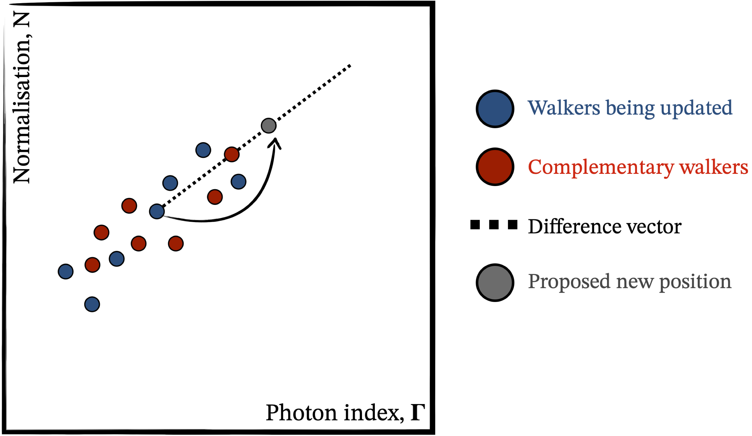
Figure 17: MCMC proposal of the affine-invariant ensemble sampler. Walkers are divided into two groups (blue and red). The blue walker paired with a red walker defines a difference vector (grey dashed), along which a new position (grey point) for the walker is proposed. The proposal is therefore oriented and scaled similar to how the walkers are already distributed. Affine transformations of the parameter space preserve the proposal.

How efficient an MCMC method is depends strongly on the proposal for the next point, or more generally the transition kernel. State-of-the-art techniques use Hamiltonian dynamics to move with high acceptance rates through the space. However, gradients of the models with respect to the parameters are necessary to achieve this, which are commonly not available in current packages. Instead, gradient-free MCMC algorithms include the popular Affine-Invariant Ensemble Sampler (AIES) from Goodman & Weare, (2010). Here, instead of a single point performing a guided random walk, a population of $K$ walkers is maintained. Half of the walkers are updated to a new random position, using information from the other half (see Figure 17). In particular, the difference vectors to a randomly paired walker is used to propose in that direction, with a random scale factor distributed around the AIES scale factor parameter $\gamma$. The proposal is accepted or rejected as described above. AIES proposes along lines, and the prior is encoded in the parameterization along which lines are drawn, or in the acceptance rule. In the case of AIES, each walker performs a guided random walk, and the random walks are interdependent because the walkers use each other as a proposal. Therefore, to diagnose the chains produced, multiple independent runs need to be performed and compared, to diagnose the runs with $\hat{R}$. See https://johannesbuchner.github.io/autoemcee/mcmc-ensemble-convergence.html for more technical details.

AIES can be well-behaved, and you should expect a few 100,000 model evaluations or more (especially for complex models) to convergence, which can be prohibitive for very slow models. AIES and in general all MCMC techniques can get stuck in local optima. For more details on MCMC and its use in X-ray spectral analysis, see van Dyk et al., (2001).

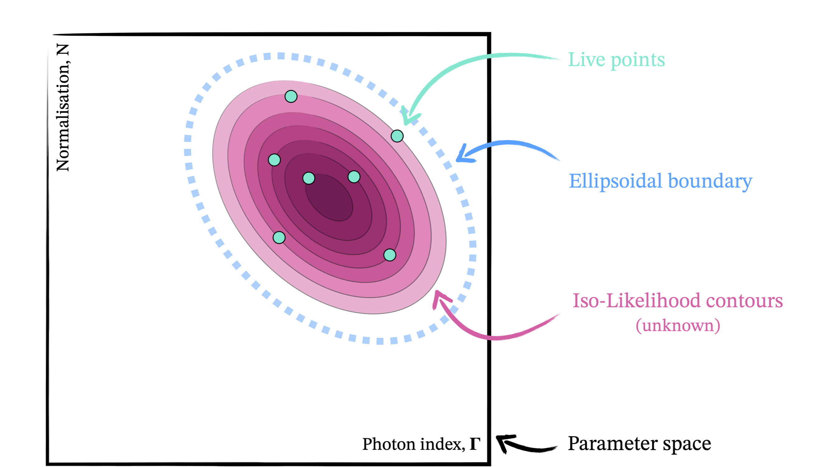
Figure 18: Ellipsoidal Nested Sampling method. The lowest likelihood live point is removed and a new sample is to be drawn, with the constraint to lie above the outer (dashed) live point contour line. However, this contour line is in general not known. Drawing from the entire prior space (black rectangle), and rejecting unsuitable points would be inefficient. Instead, an enlarged ellipsoid (blue solid line) around the existing live points (cyan circles) is constructed. Then points are proposed within the ellipsoid and accepted if above the likelihood threshold. This works very efficiently when the contours are approximately ellipsoidal.

3.4.2 Nested Sampling

Nested sampling Monte Carlo (Skilling,, 2004; Ashton et al.,, 2022) tackles the harder task of integrating the entire prior-defined parameter space. Initially, $K$ live points are sampled from the prior PDF, and are thus widely distributed across the parameter space. Most of these give very poor fits, with low likelihood ${\cal L}$. The worst (lowest likelihood) live point with ${\cal L}_{1}$ is then discarded, and a new live point sampled from the prior. However, only prior samples with ${\cal L}>{\cal L}_{1}$ are accepted as a replacement. This requirement causes approximately $1/K$ of the prior volume to be excluded. The procedure of discarding points and resampling them is repeated (nested sampling). At each iteration, the contribution to the evidence integral is estimated as $w_{i}={\cal L}_{i}V_{i}$, i.e., the likelihood weighted with the volume removed at iteration $i$, $V_{i}=\left(1-\frac{1}{K}\right)^{i}\frac{1}{K}$. The evidence is $Z_{i}\approx\sum_{i}w_{i}$, and the contribution of the live points is $Z_{\mathrm{live}}=\sum_{i}{\cal L}_{i}V_{i}$. Since each nested sampling iteration removes a poor fit and allows only better ones, after many iterations only very good fits remain. These are concentrated in a comparatively tiny volume, and have ultimately similar likelihoods, so that since $V\rightarrow 0$, $Z_{\mathrm{live}}\rightarrow 0$ and therefore $Z_{i}$ stabilizes and the iterating can be stopped. Posterior samples of equal weight are produced by randomly sampling the discarded points proportional to $w_{i}$.

The difficult task of drawing a new live point under the restriction that the likelihood must improve can be solved (see Buchner, 2021a, , for a review) by sampling in the neighbourhood of the live points. Figure 18 illustrates placing one ellipsoid around them and sampling from the ellipsoid, while rejecting proposals below the likelihood threshold (Mukherjee et al.,, 2006). Clustering into multiple ellipsoids can be even more efficient (Shaw et al.,, 2007; Feroz & Hobson,, 2008; Buchner,, 2016). When the number of model parameters becomes large, MCMC can be employed for this task inside nested sampling (Skilling,, 2004; Handley et al.,, 2015), known as step samplers. Both region sampling and step samplers are available through the Bayesian X-ray Analysis (BXA) package (Buchner, 2022b, ). For nested sampling, you should also expect a few 100,000 model evaluations or more until completion.

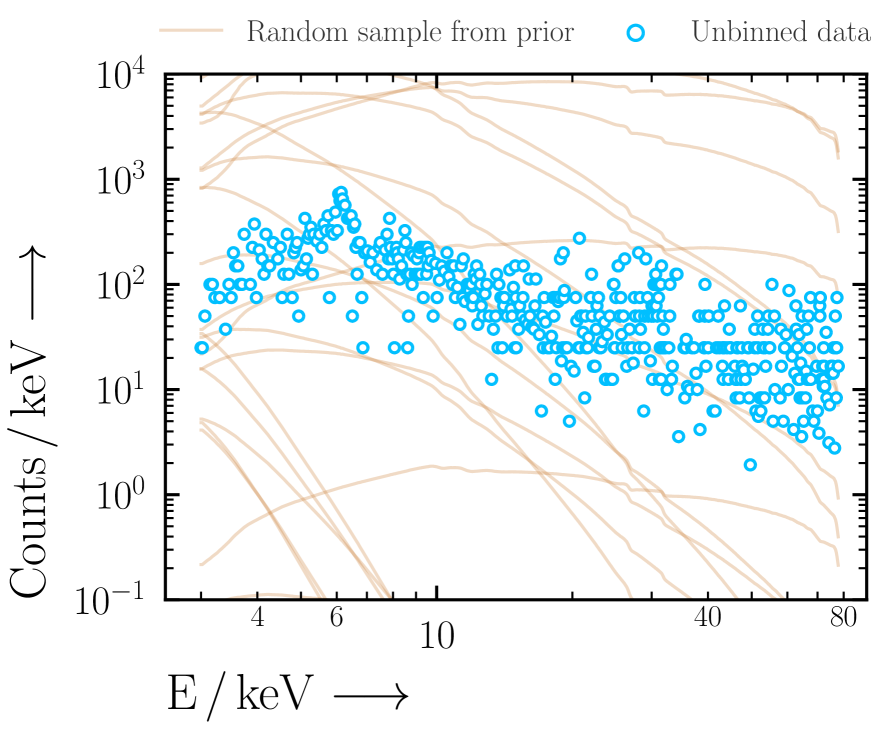
Figure 19: Prior predictive checks. Prior predictive checks are used to ensure the prior makes physical sense with regard to the data. By randomly sampling from the prior, we can see that the model is physically reasonable and is somewhat capable of producing the approximate shape of the data. The blue data points show the observed data.

3.5 Using posteriors

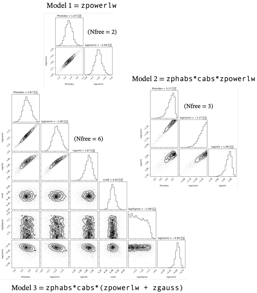
Figure 20: Corner plots created from the 3 models considered in this textbook chapter. The first two models use a redshifted power law – the first with free photon index and the second with additionally free normalisation. The second model considers an additional line-of-sight absorption component and the third considers an further redshifted Gaussian line. In all corner plots, marginal posterior probability distributions are in the diagonal and pair-wise conditional posterior distributions (for models with $>$ 1 free parameter) on the bottom left. The titles show median and $1\sigma$ equivalent quantiles of the distribution. The contours enclose 12, 39, 68 and 86 per cent of the posterior probability (see https://corner.readthedocs.io/en/latest/pages/sigmas/).

Exercise 9.2 illustrates how to obtain posteriors for the model parameters. Figure 20 shows corner plots, which include one-dimensional histograms of the posterior samples (in the diagonal of the corner plot), and two-dimensional histograms, also known as marginal posterior distributions and conditional posterior distributions, respectively. Each parameter constraint is summarized, using the quantiles corresponding to the median and 1-sigma equivalent of the marginal posterior distribution (i.e. 50, 16 and 84 percentiles). The fraction of posterior samples above or below a threshold can be used to probabilistically answer interesting questions about where the true (unknown) value lies, and where it does not (see 2.5).

But posteriors can do more than this. With the posterior $P(\theta|D)$, you can obtain uncertainties on any function that depends on $\theta$. Exercise 11 illustrates this by obtaining uncertainties on a line equivalent width from Gaussian line and powerlaw continuum parameter posteriors. For example, we can get a probabilistic prediction on the source model by computing:

$$F(E)=\int F(E|\theta)\times P(\theta|D)\,d\theta$$ (15)

This provides a view of the emission process occurring without folding through the instrument response $F(E|\theta)$ (the ‘unfolded’ model). With this, we can predict uncertainties on a flux in another energy band, perhaps observed by a future experiment. In practical terms, we take one posterior sample, compute something and obtain a prediction. Taking the ensemble of predictions over a large number of randomly-sampled posterior samples can be summarized with uncertainties, as illustrated in Figures 21 and 22.

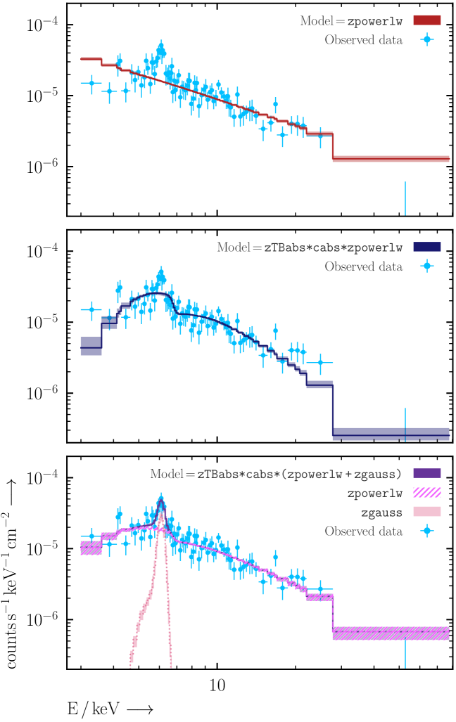
Figure 21: A plot of the folded model for each of model 1, 2 and 3. The posterior model range derived with BXA is shown as a shaded region on the model, together with the data points in each channel. The x-axis shows the nominal channel energy, and the y-values have been multiplied to correct for the bin width (keV), exposure time (s) and sensitive detector area (cm^-2). The last step lets the powerlaw source model (top panel) appear as an approximately straight line.

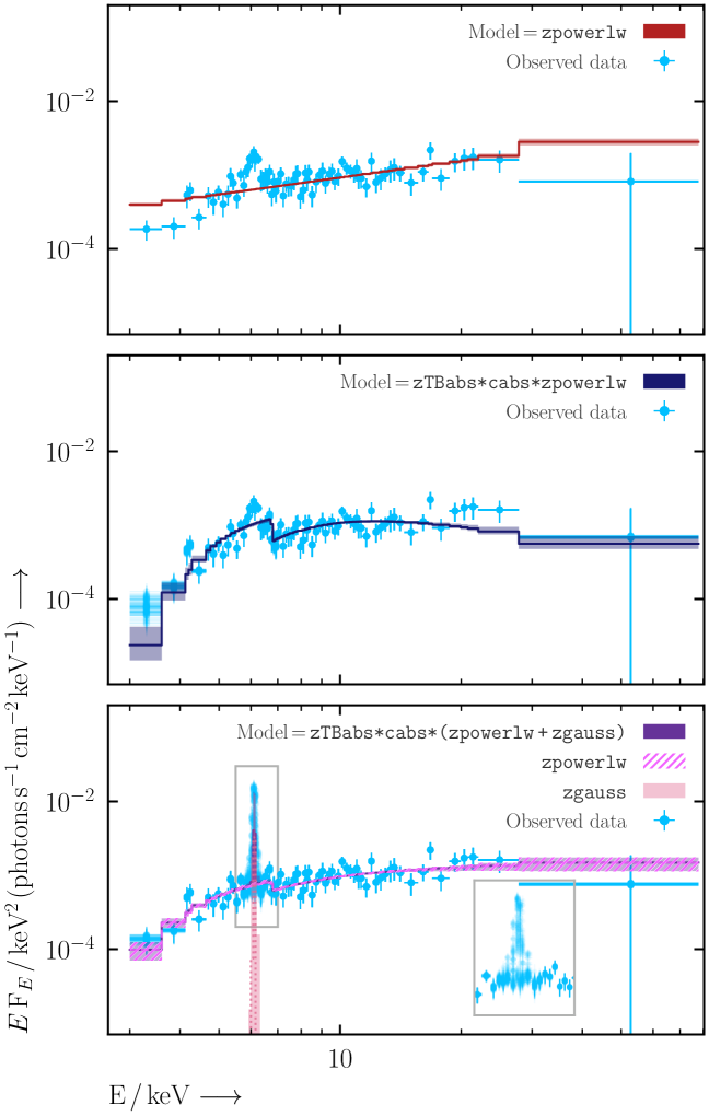
Figure 22: Flux density plots with model realisations drawn from the posteriors samples. The plotted ”data points” here depends on the data and the model, so here we show each posterior realisation of the ‘data’ in the plot. Introducing the narrow Gaussian feature in the third panel modifies the location of the data points. This highlights the possible issues in interpreting component strengths in unfolded units.

3.6 Model checking

Similar to the model checking section above, here we can take each $\theta$ with its associated probability and predict model counts $c_{i}^{\prime}$. Comparing the predicted model counts to the observed model counts, using for example $3\sigma$ intervals, is called posterior predictive checks (PPC).

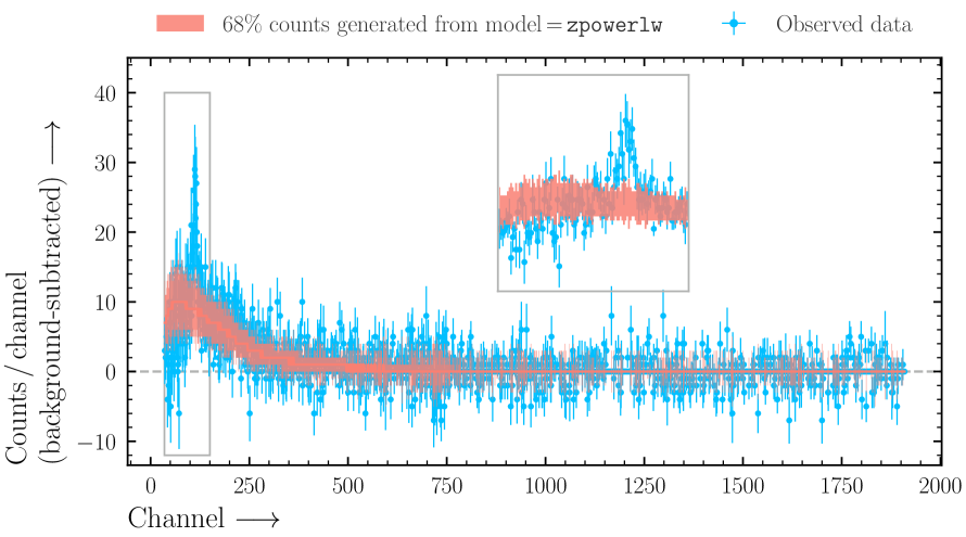
Figure 23: Model discovery with posterior predictive checks (PPC). The observed data is shown in linear counts vs. channel with red errorbars. A number of posterior rows were sampled many times from a simple power law fit and data was simulated using the same conditions as the observed data (i.e. the same exposure, response, background file). The result is shown with a red filled region. As seen in the inset, at low channel values, there appears to be a deficit and surplus in counts at channels $\sim$ 25 – 80 and 80 – 110, respectively as compared to the expected data if it were created from a power law.

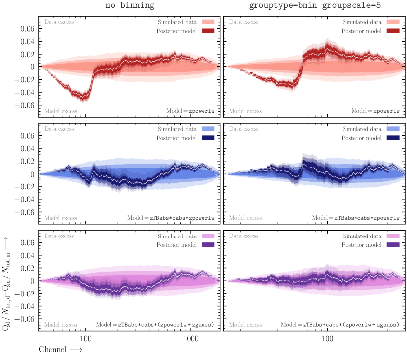
Figure 24: Q – Q difference $+$ posterior predictive checks. In each row, a different model is considered in the plane of energy vs. cumulative difference between the data and model counts (normalised by their totals, respectively). We consider two types of binning: no binning and background binning with 5 counts per background bin minimum on the left and right columns, respectively. In each panel, the horizontal shaded region shows the range that arises purely from fluctuations in the data, when simulated from the model being considered (lower right of each panel). The thin white line and darker, more irregular region then shows the resulting posterior found when fitting the model to the observed data only. In every panel, the shaded regions are separated by opacity with darker to lighter regions showing the 68%, 90% and 99% interquantile ranges. The over-estimation of the source model flux that arises from using Wstat on data that is insufficiently binned is visible in the unbinned (left column), with all model posterior ranges showing a model excess on average relative to the right column.

3.7 Model comparison

Bayes’ theorem can be applied once more: If we state the posterior of model i out of a set of competing models as

$$P(\theta|D,M_{i})=\frac{P(D|\theta,M_{i})P(\theta|M_{i})}{P(D|M_{i})}$$ (16)

then the Bayesian evidence looks like a likelihood $P(D|M_{i})$. Indeed, it is known as the total marginal likelihood, where all parameters have been marginalised out. Applying Bayes’ theorem once more we have:

$$P(M_{i}|D)=\frac{P(D|M_{i})P(M_{i})}{P(D)}$$ (17)

where $P(D)=\sum_{i}P(M_{i}|D)P(M_{i})$ normalises the set of models $\{M_{1},M_{2},\ldots\}$. What this means is that we can compute the relative probability of each model, $P(M_{i}|D)$, given computed model evidence values $Z_{i}=P(D|M_{i})$ and assumed model priors $P(M_{i})$. If we find $Z_{A}=10^{6}\times Z_{B}$ for example, then almost independent of the model priors, the resulting posterior model probability for model B will be close to zero, and hence model B is strongly disfavored.

In the case of comparing only two models, one can look at the probability ratios:

$$\underbrace{\frac{P(M_{A}|D)}{P(M_{B}|D)}}_{\mathrm{posterior~{}odds}}=\underbrace{\frac{P(M_{A})}{P(M_{B})}}_{\mathrm{prior~{}odds}}\times\underbrace{\frac{Z_{A}}{Z_{B}}}_{\mathrm{Bayes~{}factor}}$$ (18)

Bayesian model comparison allows weighing the probability of two or more models. It considers the entire parameter space, with weighting according to the prior. This has an interesting effect: Flexible models produce very diverse predictions that are excluded by the specific data and thus receive low likelihoods over most of the parameter space. This reduces the integral $Z$, since that is an average over the parameter space. Therefore, Bayesian model comparison prefers simpler models (Occam’s razor). Simpler is not defined by the number of parameters, but by the diversity of predictions of the model.

Bayesian inference gives relative probabilities. It does not make decisions. If we make a decision, for example, discarding the model with lower probability (e.g., $Z_{A}>Z_{B}$ in a priori equally probable models), we do not know the false positive rate and false negative rate of this decision process. However, we can apply the process as described in the frequentist ‘model comparison’ section (Section 2.4): Given our indicator $Z_{A}/Z_{B}$, simulate under the null model, identify a threshold corresponding to a desired false positive rate, and apply this with confidence. This has the benefit of interpretability of the result in a Bayesian sense and simultaneously a purity guarantee. The main drawback is that the computation of $Z$ for several hundred simulated spectra can take a long time. Nevertheless, Baronchelli et al., (2018) demonstrated such false positive and false negative computations with BXA for detecting relativistically broadened Fe K lines.

To overcome computational difficulties, approximation to the evidence integral have been proposed. This includes, in order of decreasing quality, the Laplace approximation, which considers the parameter uncertainties and the BIC (Bayesian information criterion), which only considers the maximum likelihood value. Both approximations break down close to the parameter boundaries, and with non-Gaussian posteriors.

The Akaike Information Criterion (AIC), and its variants (Deviance Information Criterion, Widely Applicable Information Criterion) are not based on Bayesian inference. Instead, they compare models based on the information lost when storing the model parameters instead of the data. Better models (with lower information criterion value), thus more completely describe the data. They are useful especially for comparing auxiliary, ad-hoc, empirical models that do not aim to describe the underlying physical process of interest.

4 Parameter distributions of a sample

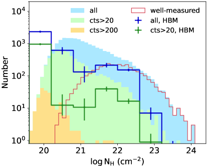
Figure 25: Hierarchical Bayesian Modelling in practice. The blue filled histogram shows the distribution of the median $N_{H}$ posteriors measured in 20,000 AGN. Even for sources with $\log N_{\mathrm{H}}=20$, the median is higher than 20 because of measurement uncertainties extending the posterior from 20 to 22 or 23, depending on the counts obtained. Considering only sources above some source count threshold, the distribution is more concentrated towards 20. The blue step histogram shows the result from the hierarchical Bayesian model (HBM), considering both the sample distribution and the measurement uncertainties of each source. This shows the sample distribution, subject to selection effects, not the distribution of the underlying population. From Liu et al., (2022) with permission from Teng Liu.

Finally, let’s say you have observed not just the spectrum of one source, but of several sources from a survey. You notice that each source has a slightly different $\Gamma$ (each measured with uncertainties). Now you want to determine the distribution of $\Gamma$ in this sample. A simple approach here would be to plot a histogram of the best-fit $\Gamma$ (optima), or the mean or medians of the posterior PDF. However, this does not consider the uncertainties. This is especially problematic when the uncertainties are diverse, which is usually the case.

Diverse uncertainties cause an interesting effect in such histograms. While the $\hat{\theta}$ estimator from sources with small error bars will be stable, those with large error bars dilute the histogram by their scatter. So the histogram shows the intrinsic dispersion of the sample convolved and broadened by dispersion due to statistical effects. A real-world example is shown in Figure 25. We would really like to separate out the measurement effect and obtain plausible sample distributions.

That is not trivial with the frequentist approach. In the Bayesian approach, this is addressed with hierarchical (or multi-level) models.

Let’s assume that the true sample distribution of $\theta$ is a Gaussian with mean $\mu$ and standard deviation $\sigma$. Then we can replace the prior $\pi(\theta)$ with this population model $G(\theta|\mu,\sigma)$ in eq. 12. We obtain an extended posterior which includes the population model parameters and the per-source parameters $\theta_{i}$:

$$P(\theta_{i},\mu,\sigma|D)\propto\prod_{i}{\cal L}(\theta_{i})\times G(\theta_{i}|\mu,\sigma)\times\pi(\mu,\sigma)$$ (19)

Now, we are analysing all objects simultaneously. Each object has free parameters, but at the same time these free parameters are linked by the Gaussian population distribution. Then, we can sample posteriors and obtain marginal posterior distributions for $\mu$ and $\sigma$ to learn about the true distribution. This marginalises over the uncertainties in each object.

How can this be implemented in X-ray spectral fitting packages? Not trivially, but a numerical approximation is possible. If per-source posteriors were obtained under flat priors in the parameter of interest, then the posterior of the population parameters can be approximated as:

$$P(\mu,\sigma|D)\propto\prod_{i}\sum_{j}G(\theta_{ij}|\mu,\sigma)\times\pi(\mu,\sigma)$$ (20)

Here, the per-source parameters $\theta_{i}$ have been marginalized out by averaging over the posterior samples, which are assumed to be of equal length across the objects. The PosteriorStacker package (Baronchelli et al.,, 2018) implements this numerical approach for inferring one-dimensional sample distributions, with a Gaussian population model and a more flexible histogram-like population model.

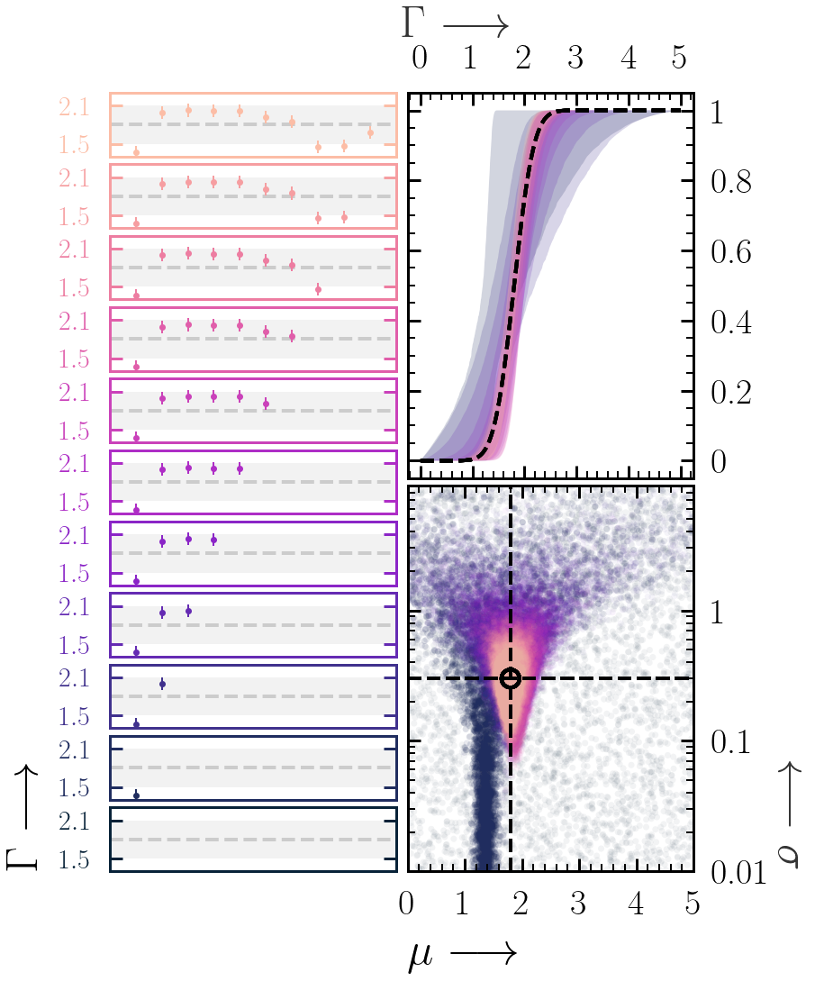
Figure 26: Behaviour of single-parameter Hierarchical Bayesian Model. A set of 0 to 10 sources is considered (left panels), for each source, a parameter $\Gamma$ was constrained (error bar). We seek to determine the true sample distribution. In this case, it is a Gaussian, with the mean and standard deviation illustrated with the dashed gray line and shade. For each panel with its color, one PosteriorStacker sample analysis was performed. For the assumed Gaussian sample distribution model, this constrains the mean and standard deviation parameters. Plausible distributions (top right panel), according to posterior samples (bottom right panel), are illustrated with corresponding colors. The truth is shown with a dashed black line.

Inferring population demographics, that is, correcting for selection effects when the sample was obtained is beyond the scope of this chapter. For the extension of hierarchical modelling to include sample selection effects see for example (Loredo,, 2004; Loredo & Hendry,, 2019).

5 Further information

Books on Statistics

• "Introduction to Probability" (Dimitri Bertsekas): covers basics: random variables, combinatorics, derived distributions, what is a PDF, how to work with them, expectation values

• "Probability and Statistics" (Morris H. DeGroot): covers classical approaches to hypothesis testing and frequentist analysis, so you can really understand, e.g., the classical tests, what p-values really are, why they are used and how and when they are useful.

• "Scientific Inference" (Simon Vaughan): basic probability theory, statistical thinking, model and data representation in computers, likelihood function, graphical summaries, basic Monte Carlo.

• "Data Analysis - A Bayesian Tutorial" (Sivia): building an intuition for how Bayesian statistics works

• "Bayesian data analysis" (Gelman): http://www.stat.columbia.edu/~gelman/book/

Links

• A living repository for the figures and exercises used in this Chapter https://github.com/pboorm/xray_spectral_fitting

• ‘Statistics in XSpec’ manual https://heasarc.gsfc.nasa.gov/xanadu/xspec/manual/XSappendixStatistics.html

• Astrostatistics Facebook group: https://www.facebook.com/groups/astro.r/

• XSpec group: https://www.facebook.com/groups/320119452570/

• International CHASC Astro-Statistics Collaboration: http://hea-www.harvard.edu/AstroStat/

• X-ray Spectral Fitting tutorial: http://peterboorman.com/tutorial_bxa.html

Software packages

• Sherpa/CIAO: https://cxc.harvard.edu/sherpa/

• XSpec/HEASoft: https://heasarc.gsfc.nasa.gov/lheasoft/

• BXA (Nested Sampling for XSpec or Sherpa): https://johannesbuchner.github.io/BXA/

• SPEX: https://www.sron.nl/astrophysics-spex

• ISIS: https://space.mit.edu/CXC/ISIS/

• 3ML: https://threeml.readthedocs.io/

References

- Andrae et al., (2010) Andrae, R., Schulze-Hartung, T., & Melchior, P. (2010). Dos and don’ts of reduced chi-squared. arXiv e-prints, (pp. arXiv:1012.3754).
- Ashton et al., (2022) Ashton, G., Bernstein, N., Buchner, J., Chen, X., Csányi, G., Fowlie, A., Feroz, F., Griffiths, M., Handley, W., Habeck, M., Higson, E., Hobson, M., Lasenby, A., Parkinson, D., Pártay, L. B., Pitkin, M., Schneider, D., Speagle, J. S., South, L., Veitch, J., Wacker, P., Wales, D. J., & Yallup, D. (2022). Nested sampling for physical scientists. arXiv e-prints, (pp. arXiv:2205.15570).
- Baronchelli et al., (2018) Baronchelli, L., Nandra, K., & Buchner, J. (2018). Relativistic reflection from accretion discs in the population of active galactic nuclei at z = 0.5-4. MNRAS, 480(2), 2377–2385.
- Buchner, (2016) Buchner, J. (2016). A statistical test for Nested Sampling algorithms. Statistics and Computing, 26(1-2), 383–392.
- (5) Buchner, J. (2021a). Nested Sampling Methods. arXiv e-prints, (pp. arXiv:2101.09675).
- (6) Buchner, J. (2021b). Nested Sampling Methods. arXiv e-prints, (pp. arXiv:2101.09675).
- (7) Buchner, J. (2022a). An Intuition for Physicists: Information Gain From Experiments. Research Notes of the American Astronomical Society, 6(5), 89.
- (8) Buchner, J. (2022b). Comparison of Step Samplers for Nested Sampling. arXiv e-prints, (pp. arXiv:2211.09426).
- Buchner et al., (2014) Buchner, J., Georgakakis, A., Nandra, K., Hsu, L., Rangel, C., Brightman, M., Merloni, A., Salvato, M., Donley, J., & Kocevski, D. (2014). X-ray spectral modelling of the AGN obscuring region in the CDFS: Bayesian model selection and catalogue. A&A, 564, A125.
- Cash, (1979) Cash, W. (1979). Parameter estimation in astronomy through application of the likelihood ratio. ApJ, 228, 939–947.
- Feroz & Hobson, (2008) Feroz, F. & Hobson, M. P. (2008). Multimodal nested sampling: an efficient and robust alternative to Markov Chain Monte Carlo methods for astronomical data analyses. MNRAS, 384, 449–463.
- Fioretti & Bulgarelli, (2020) Fioretti, V. & Bulgarelli, A. (2020). How to Detect X-Rays and Gamma-Rays from Space: Optics and Detectors; Data Reduction and Analysis. In Fundamental Concepts; Data Reduction and Analysis. Edited by Cosimo Bambi. ISBN: 978-981-15-6336-2. Springer (pp. 55–117).
- Gelman & Rubin, (1992) Gelman, A. & Rubin, D. B. (1992). A single series from the gibbs sampler provides a false sense of security. Bayesian statistics, 4, 625–631.
- Goodman & Weare, (2010) Goodman, J. & Weare, J. (2010). Ensemble samplers with affine invariance. Communications in Applied Mathematics and Computational Science, Vol. 5, No. 1, p. 65-80, 2010, 5, 65–80.
- Handley et al., (2015) Handley, W. J., Hobson, M. P., & Lasenby, A. N. (2015). POLYCHORD: nested sampling for cosmology. MNRAS, 450, L61–L65.
- Humphrey et al., (2009) Humphrey, P. J., Liu, W., & Buote, D. A. (2009). 2 and Poissonian Data: Biases Even in the High-Count Regime and How to Avoid Them. ApJ, 693(1), 822–829.
- Kaastra, (2017) Kaastra, J. S. (2017). On the use of C-stat in testing models for X-ray spectra. A&A, 605, A51.
- Kaastra & Bleeker, (2016) Kaastra, J. S. & Bleeker, J. A. M. (2016). Optimal binning of X-ray spectra and response matrix design. A&A, 587, A151.
- Liu et al., (2022) Liu, T., Buchner, J., Nandra, K., Merloni, A., Dwelly, T., Sanders, J. S., Salvato, M., Arcodia, R., Brusa, M., Wolf, J., Georgakakis, A., Boller, T., Krumpe, M., Lamer, G., Waddell, S., Urrutia, T., Schwope, A., Robrade, J., Wilms, J., Dauser, T., Comparat, J., Toba, Y., Ichikawa, K., Iwasawa, K., Shen, Y., & Medel, H. I. (2022). The eROSITA Final Equatorial-Depth Survey (eFEDS). The AGN catalog and its X-ray spectral properties. A&A, 661, A5.
- Loredo, (2004) Loredo, T. J. (2004). Accounting for Source Uncertainties in Analyses of Astronomical Survey Data. In R. Fischer, R. Preuss, & U. V. Toussaint (Ed.), American Institute of Physics Conference Series, volume 735 of American Institute of Physics Conference Series (pp. 195–206).
- Loredo & Hendry, (2019) Loredo, T. J. & Hendry, M. A. (2019). Multilevel and hierarchical Bayesian modeling of cosmic populations. arXiv e-prints, (pp. arXiv:1911.12337).
- Maggi et al., (2014) Maggi, P., Haberl, F., Kavanagh, P. J., Points, S. D., Dickel, J., Bozzetto, L. M., Sasaki, M., Chu, Y. H., Gruendl, R. A., Filipović, M. D., & Pietsch, W. (2014). Four new X-ray-selected supernova remnants in the Large Magellanic Cloud. A&A, 561, A76.
- Metropolis et al., (1953) Metropolis, N., Rosenbluth, A. W., Rosenbluth, M. N., Teller, A. H., & Teller, E. (1953). Equation of State Calculations by Fast Computing Machines. Journal of Chemical Physics, 21(6), 1087–1092.
- Mighell, (1999) Mighell, K. J. (1999). Parameter Estimation in Astronomy with Poisson-distributed Data. I.The 2γ Statistic. ApJ, 518(1), 380–393.
- Mukherjee et al., (2006) Mukherjee, P., Parkinson, D., & Liddle, A. R. (2006). A Nested Sampling Algorithm for Cosmological Model Selection. ApJ, 638, L51–L54.
- Nousek & Shue, (1989) Nousek, J. A. & Shue, D. R. (1989). Psi 2 and C Statistic Minimization for Low Count per Bin Data. ApJ, 342, 1207.
- Protassov et al., (2002) Protassov, R., van Dyk, D. A., Connors, A., Kashyap, V. L., & Siemiginowska, A. (2002). Statistics, Handle with Care: Detecting Multiple Model Components with the Likelihood Ratio Test. ApJ, 571, 545–559.
- Ricci et al., (2017) Ricci, C., Trakhtenbrot, B., Koss, M. J., Ueda, Y., Del Vecchio, I., Treister, E., Schawinski, K., Paltani, S., Oh, K., Lamperti, I., Berney, S., Gandhi, P., Ichikawa, K., Bauer, F. E., Ho, L. C., Asmus, D., Beckmann, V., Soldi, S., Baloković, M., Gehrels, N., & Markwardt, C. B. (2017). BAT AGN Spectroscopic Survey. V. X-Ray Properties of the Swift/BAT 70-month AGN Catalog. ApJS, 233(2), 17.
- Shaw et al., (2007) Shaw, J. R., Bridges, M., & Hobson, M. P. (2007). Efficient Bayesian inference for multimodal problems in cosmology. MNRAS, 378, 1365–1370.
- Simmonds et al., (2018) Simmonds, C., Buchner, J., Salvato, M., Hsu, L. T., & Bauer, F. E. (2018). XZ: Deriving redshifts from X-ray spectra of obscured AGN. A&A, 618, A66.
- Skilling, (2004) Skilling, J. (2004). Nested sampling. AIP Conference Proceedings, 735(1), 395.
- van Dyk et al., (2001) van Dyk, D. A., Connors, A., Kashyap, V. L., & Siemiginowska, A. (2001). Analysis of Energy Spectra with Low Photon Counts via Bayesian Posterior Simulation. ApJ, 548(1), 224–243.
- Vehtari et al., (2019) Vehtari, A., Gelman, A., Simpson, D., Carpenter, B., & Bürkner, P.-C. (2019). Rank-normalization, folding, and localization: An improved for assessing convergence of MCMC. arXiv e-prints, (pp. arXiv:1903.08008).
- Wachter et al., (1979) Wachter, K., Leach, R., & Kellogg, E. (1979). Parameter estimation in X-ray astronomy using maximum likelihood. ApJ, 230, 274–287.
- Wheaton et al., (1995) Wheaton, W. A., Dunklee, A. L., Jacobsen, A. S., Ling, J. C., Mahoney, W. A., & Radocinski, R. G. (1995). Multiparameter Linear Least-Squares Fitting to Poisson Data One Count at a Time. ApJ, 438, 322.
- Wik et al., (2014) Wik, D. R., Lehmer, B. D., Hornschemeier, A. E., Yukita, M., Ptak, A., Zezas, A., Antoniou, V., Argo, M. K., Bechtol, K., Boggs, S., Christensen, F., Craig, W., Hailey, C., Harrison, F., Krivonos, R., Maccarone, T. J., Stern, D., Venters, T., & Zhang, W. W. (2014). Spatially Resolving a Starburst Galaxy at Hard X-Ray Energies: NuSTAR, Chandra, and VLBA Observations of NGC 253. ApJ, 797(2), 79.
- Wilks, (1938) Wilks, S. (1938). The large-sample distribution of the likelihood ratio for testing composite hypotheses. The Annals of Mathematical Statistics, (pp. 60–62).