What are the parities of photon-ring images near a black hole?

Abstract

Light that grazes a black-hole event horizon can loop around one or more times before escaping again, resulting for distance observers in an infinite sequence of ever fainter and more delayed images near the black hole shadow. In the case of the M87 and Sgr A^∗ back holes, the first of these so-called photon-ring images have now been observed. A question then arises: are such images minima, maxima, or saddle-points in the sense of Fermat’s principle in gravitational lensing? or more briefly, the title question above. In the theory of lensing by weak gravitational fields, image parities are readily found by considering the time-delay surface (also called the Fermat potential or the arrival-time surface). In this work, we extend the notion of the time delay surface to strong gravitational fields and compute the surface for a Schwarzschild black hole. The time-delay surface is the difference of two wavefronts, one travelling forward from the source and one travelling backwards from the observer. Image parities are read off from the topography of the surface, exactly as in the weak-field regime, but the surface itself is more complicated. Of the images, furthest from the black hole and similar to the weak-field limit, are a minimum and a saddle point. The strong field repeats the pattern, corresponding to light taking one or more loops around the back hole. In between, there are steeply-rising walls in the time-delay surface, which can be interpreted as maxima and saddle points that are infinitely delayed and not observable — these correspond to light rays taking a U-turn around the black hole.

1 Introduction

One of the tests of Einstein’s theory of gravity is the deflection of light rays (also known as gravitational lensing) by matter distributions [1; 2; 3]. It was first recognised in the observation of stars behind the Sun during the famous 1919 eclipse [4] and, later, in the radio observation of a distant quasar lying behind a foreground galaxy and forming multiple images [5]. Since then, light deflection has been observed from individual stars in our Galaxy to distant galaxy clusters [6; 7] and became an integral part of the study of the Universe [8; 9].

In general, a weak-field approximation (where the spacetime can be decomposed into a background and a small perturbation on this background created by the lens [10]) is sufficient to study the conventional gravitational lensing from a star, galaxy, or galaxy cluster and explain all observed properties of the lensed images [11]. However, a weak field approximation breaks down very close to a neutron star or a black hole, where light rays experience very strong gravitational fields. The existence of such objects (neutron stars and black holes) has been confirmed by different methods (for example, using x-ray binaries [12]; gravitational wave observations [13; 14]; astrometric microlensing [15]) and even black-hole shadows have been imaged for the supermassive black holes at the centre of the nearby galaxy M87 [16; 17; 18; 19] and our own Galaxy [20; 21; 22].

In the strong gravitational field near a black hole, instead of using the conventional lens equation derived using a weak-field approximation, one needs to solve the geodesic equation to determine the path of light rays. The simplest case to study light propagation in a strong gravitational field is lensing by a Schwarzschild black hole [23] (also see [24]), a classic topic in the literature. An analytical solution for the deflection angle near Schwarzschild black hole can be derived in terms of elliptic integral [25; 26; 27]. [28] and [29] obtained (approximate) gravitational lens equation applicable in strong gravitational field near the Schwarzschild black hole and discussed the presence of the infinite sequence of (increasingly de-magnified) lensed images of a background source (also known as relativistic images). Using a different formalism, [30] derived an exact lens equation for Schwarzschild black hole. Going beyond lensing by Schwarzschild black hole, similar analyses have also been performed for Kerr(-Newman) and more exotic black holes [e.g., 31; 32; 33; 34; 35].

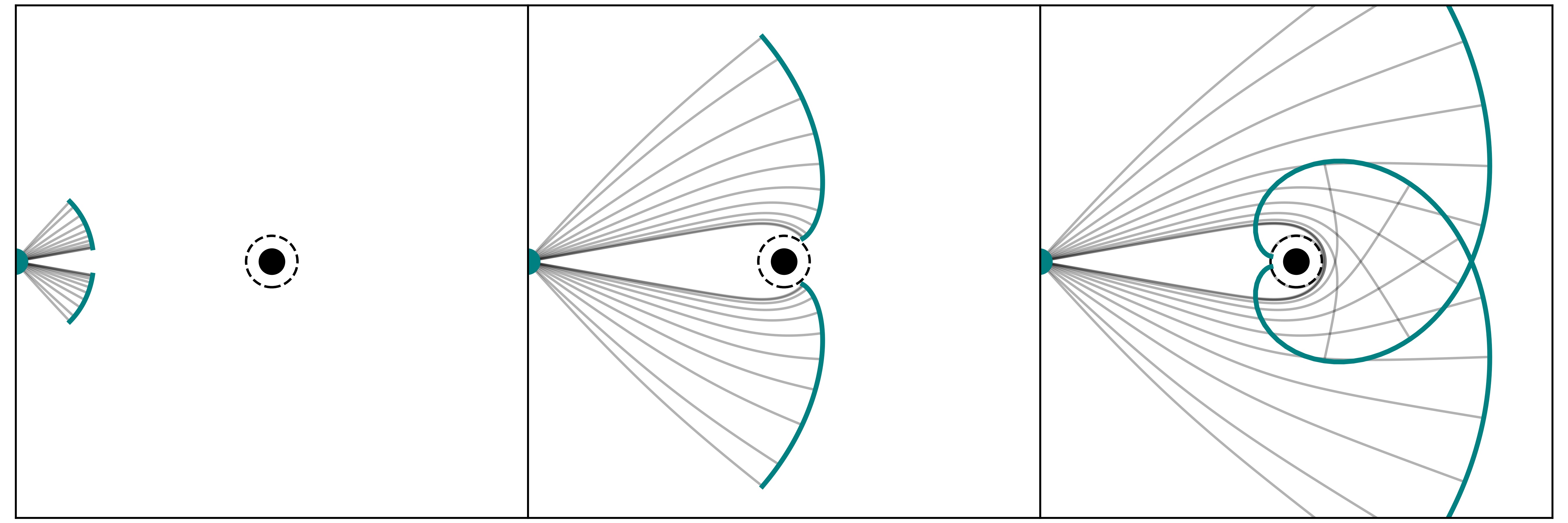
Figure 1: Wavefront propagation near a Schwarzschild black hole lens. The black dot in each panel represents the black hole position. The black dashed circle around the black hole marks the photon sphere ($r=3M$). The green dot represents the source position, and grey curves represent the light rays emitted from the source. The equal time surfaces (or wavefronts) for these rays are shown by the green curves. The left, middle, and right panels represent the wavefront for three different time values (in increasing order), respectively. In each panel, the gap in the middle of the wavefront corresponds to rays which fall inside the black hole.

A very instructive way to describe gravitational lensing is thinking in terms of wavefronts emitted from the source instead of individual light rays. The wavefront method was first used in gravitational lensing to estimate the time delay between multiple images for point mass and axially symmetric lenses to determine the Hubble constant [36; 37; 38]. For a given lens system (made of source, lens, and observer), a wavefront emitted from the source gets deformed and develops crossings as it crosses the lens and moves forward [e.g., 39]. A pedagogical introduction to wavefronts in gravitational lensing is presented in [40; 41]. The use of the wavefront method in the strong gravitational field was first discussed in [42] to construct caustic structure near a Kerr black hole. Later, the wavefront method was used in [43; 44; 45] to further understand the light propagation near Kerr black hole and in other (more exotic) spacetimes [e.g., 46].

In the contemporary literature on lensing in the weak field limit, the time delay surface is a fundamental quantity which can be used to describe the various properties of the lensed images like position, magnification, and parity [47]. For strong fields, there is a general formulation of Fermat’s principle [48], but the weak-field time-delay surface has not been generalised. There is, however, an elegant construction using wavefronts [40; 41], which can be adapted. In our current work, we use wavefronts to compute time delay surfaces near the Schwarzschild black hole for axially and non-axially symmetric cases. Since the images are essentially extrema points of the time delay surface, we can infer that even in the strong gravitational field, the lensed images should be either minima or maxima, or saddle-point. However, to determine the exact order in which these different types of images will appear is not obvious. In addition, a Schwarzschild black hole is a singular lens. This can lead to tears in the time delay surface similar to the point mass lens in weak field limit and make the overall geometry of the time delay surface very complex near the black hole. Hence, an explicit construction of time delay surface near the black hole is necessary to address the above issues.

The current work is organised as follows. In Section 2, we briefly discuss the light propagation and wavefronts near the Schwarzschild black hole. In Section 3, we construct the time delay surface for axis-symmetric case (i.e., when the source lies on the optical axis, a line joining the observer and lens) and discuss the parity of the lensed images near the Schwarzschild black hole. In Section 4, similarly, we construct the time delay surface and determine the parities for an off-axis source. Section 5, discusses the formation of infinitely delayed images in between different pairs of observed images. We conclude our work in Section 6. Throughout this work, we use the natural unit system, ($c=1,\>G=1$), unless mentioned otherwise.

2 Light paths past a Schwarzschild lens

The trajectory of photons passing near the Schwarzschild black hole are determined by the following equations,

$${dr\over dt} =\left(1-\frac{2M}{r}\right)\sqrt{1-\frac{b^{3}}{b-2M}{r-2M\over r^{3}}},$$ (1)

$${d\phi\over dt} =\left(1-\frac{2M}{r}\right){1\over r^{2}}\sqrt{{b^{3}\over b-2M}},$$

where $r=b$ is the distance of close approach and $(t,r,\phi)$ are the spacetime coordinates in the plane where the light travels (i.e., $\theta=\pi/2$). We refer readers to Appendix A describing a method to derive the above equations and Appendix B for various limiting cases of the above equations.

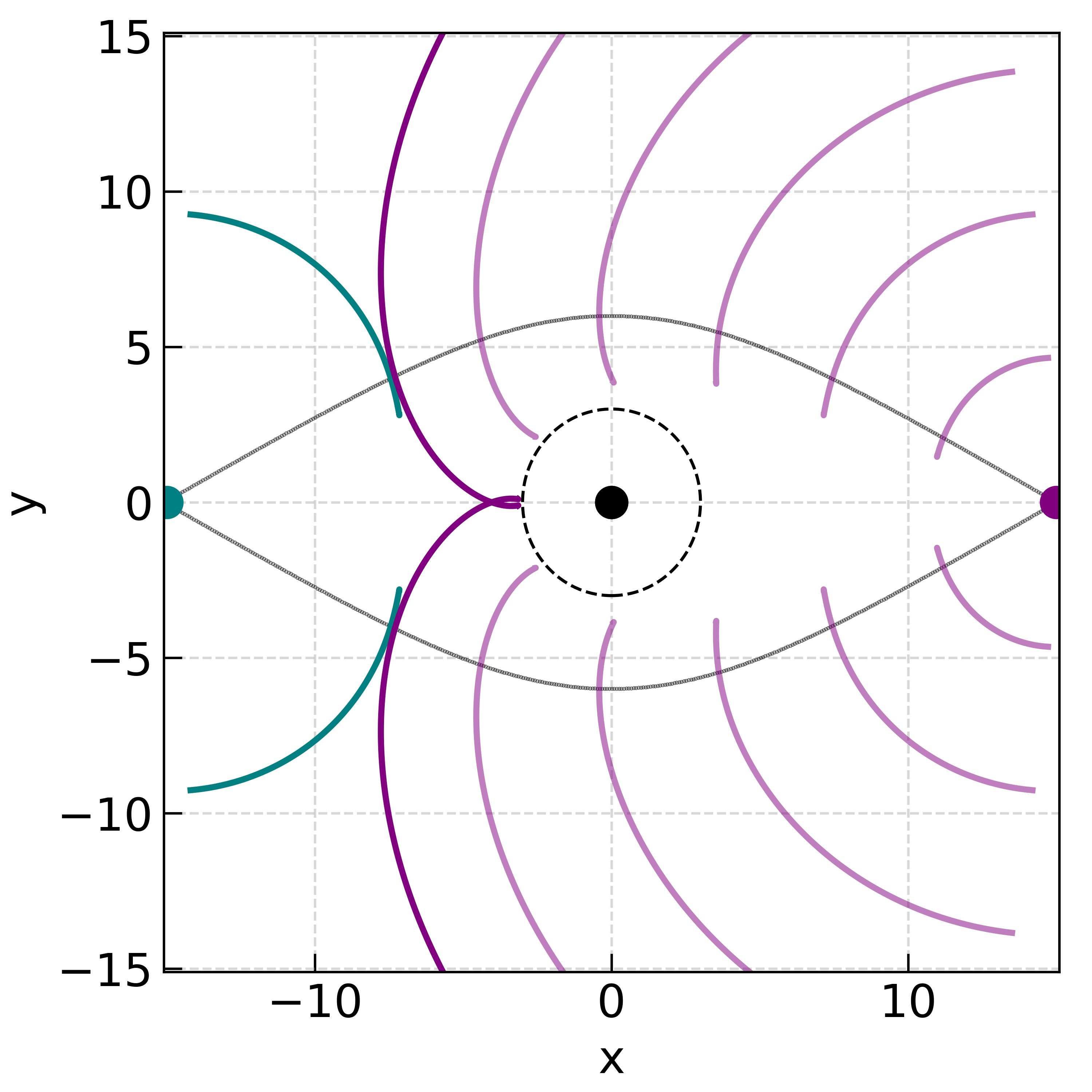
Figure 2: Wavefront propagation near a Schwarzschild black hole in the axially symmetric case. The green, black and purple dots represent the position of the source, lens, and observer, respectively. The green curves represent the wavefront emitted by the source. The purple curves represent a wavefront emitted from the observer at different time instances. The lensed images correspond to points on the purple and green wavefronts where their normal vector agree with each other. These points are essentially the points in the figure where purple and green wavefronts touch each other. The grey curves represent the corresponding rays emitted from the source and reach to the observer.

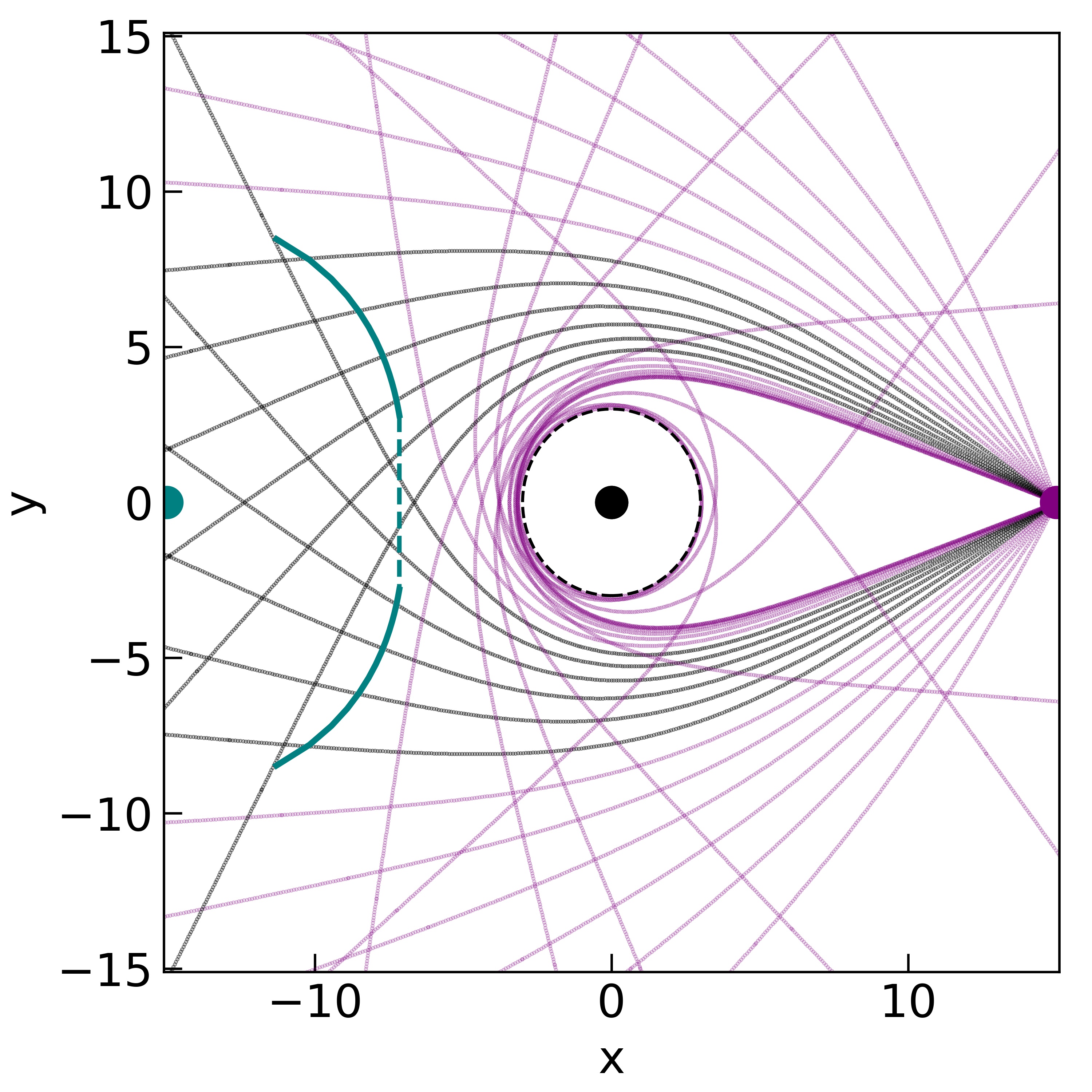
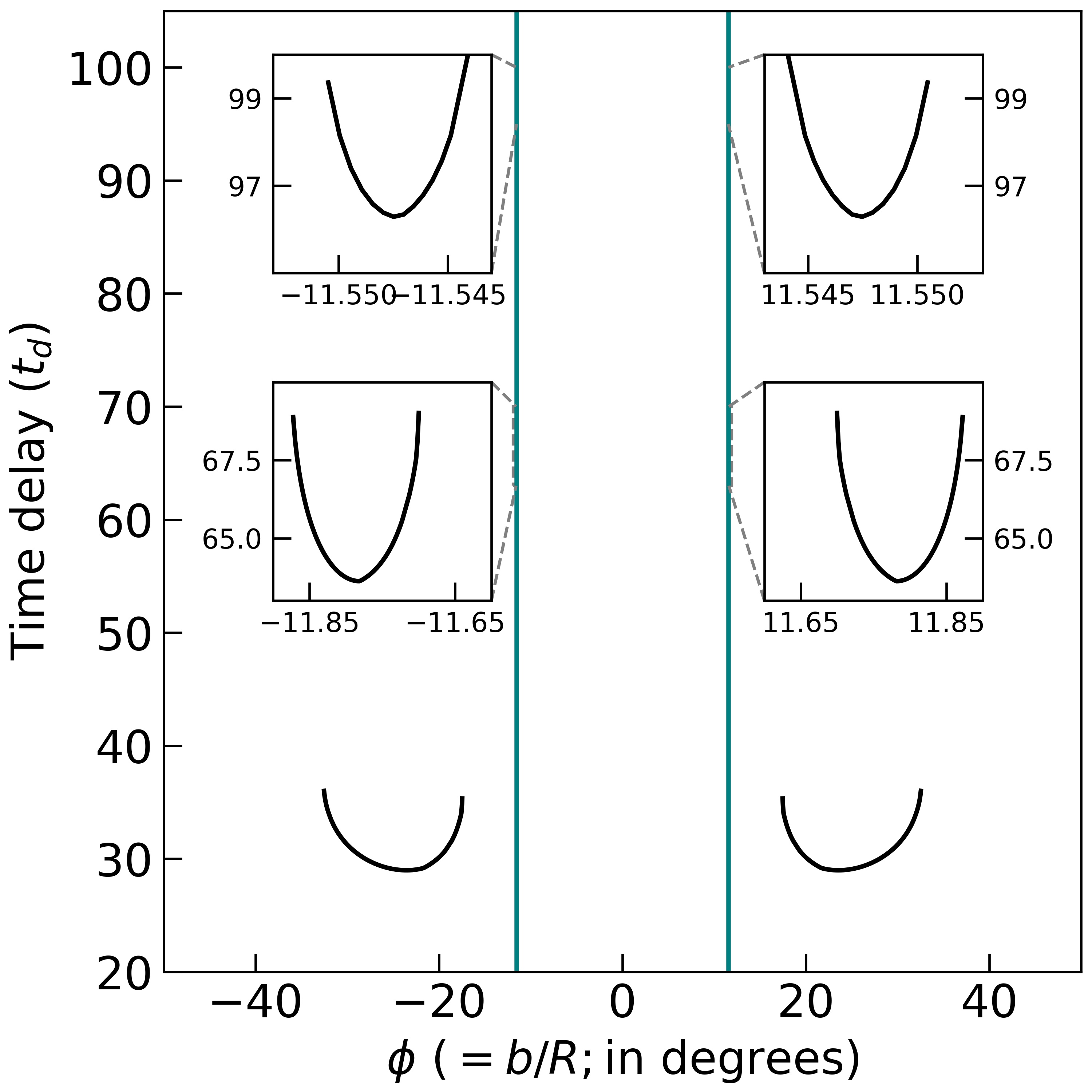
Figure 3: Construction of a time delay surface near a Schwarzschild black hole for the axially symmetric case. Left panel: The green, black, and purple dots at (-15, 0), (0,0), and (0,15) represent the position of source, Schwarzschild black hole, and observer, respectively. The black dashed line represents the photon sphere ($r=3$) around the black hole. The green curve represents the wavefront emitted by the source. The grey (purple) curves mark the rays emitted from the observer, which (do not) cross the green wavefront. Right panel: Time delay ($t_{d}$; in units of $GM/c^{3}$) as a function of angle of closest approach ($\phi$; in degrees) with respect to the observer. The green vertical lines mark the angle corresponding to the photon sphere. The black curves represent the slices of time delay surface near primary, secondary, and tertiary images as we go from small to large time delays. For time delays near the secondary and tertiary images, we show zoom-in plots since the images form very close to the photon sphere.

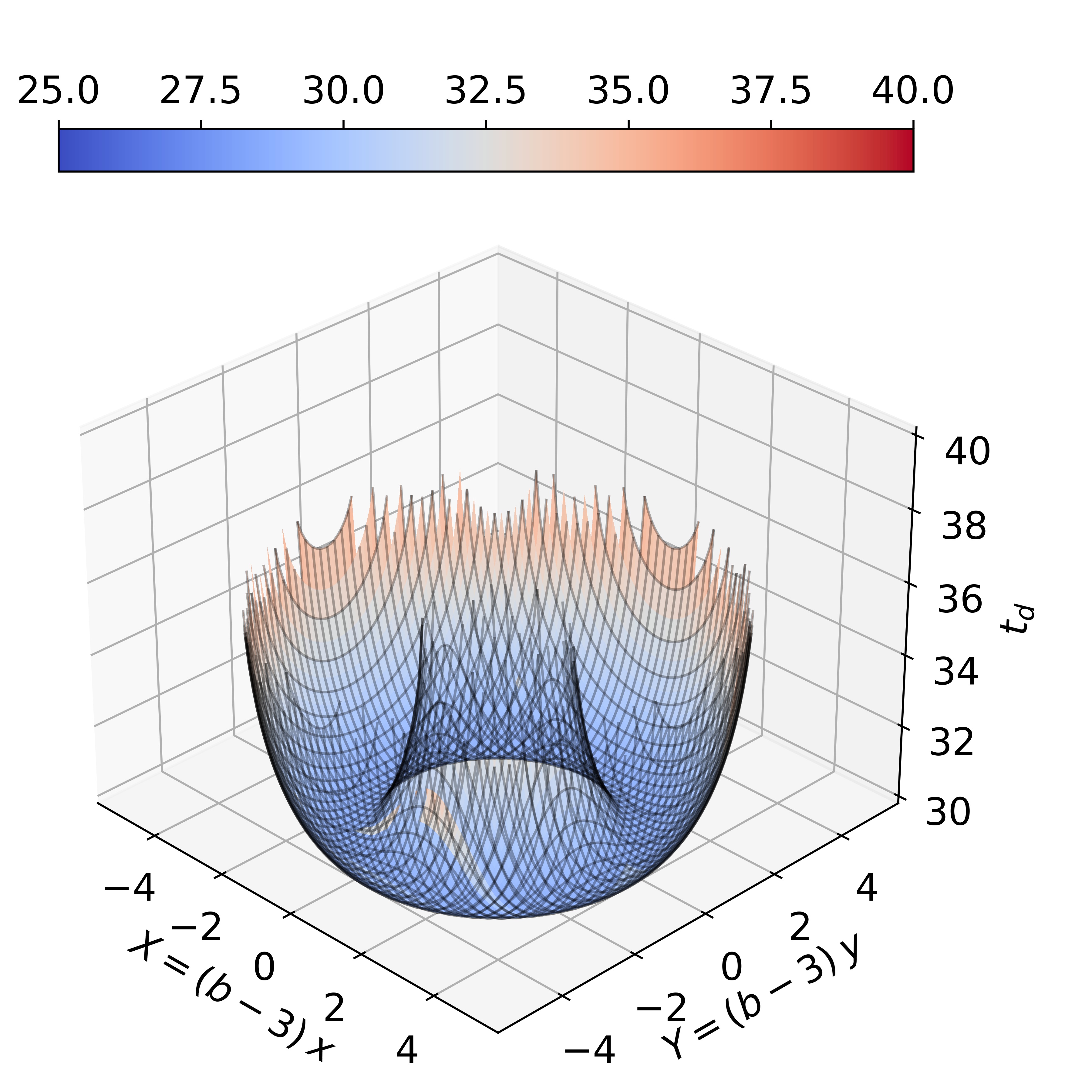
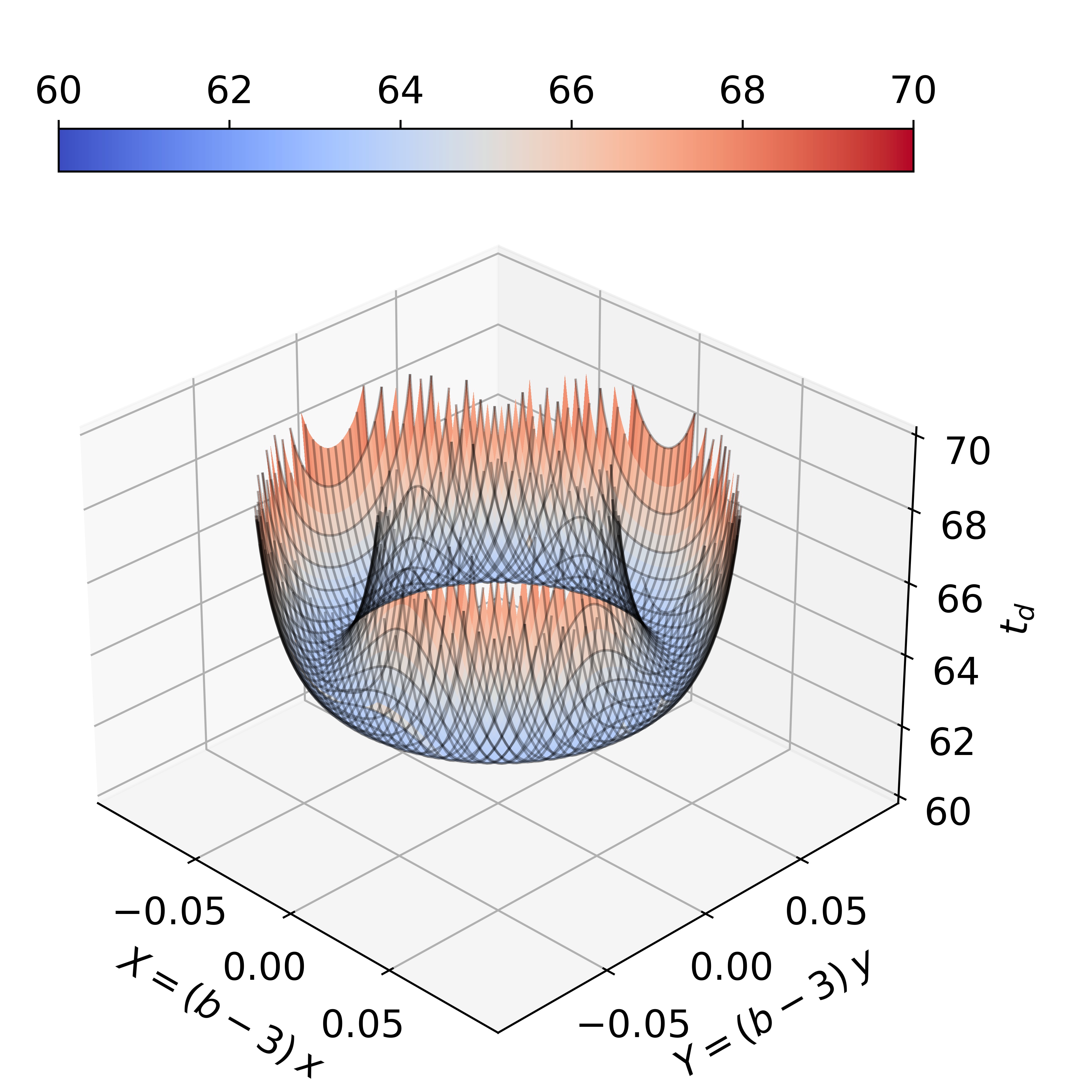
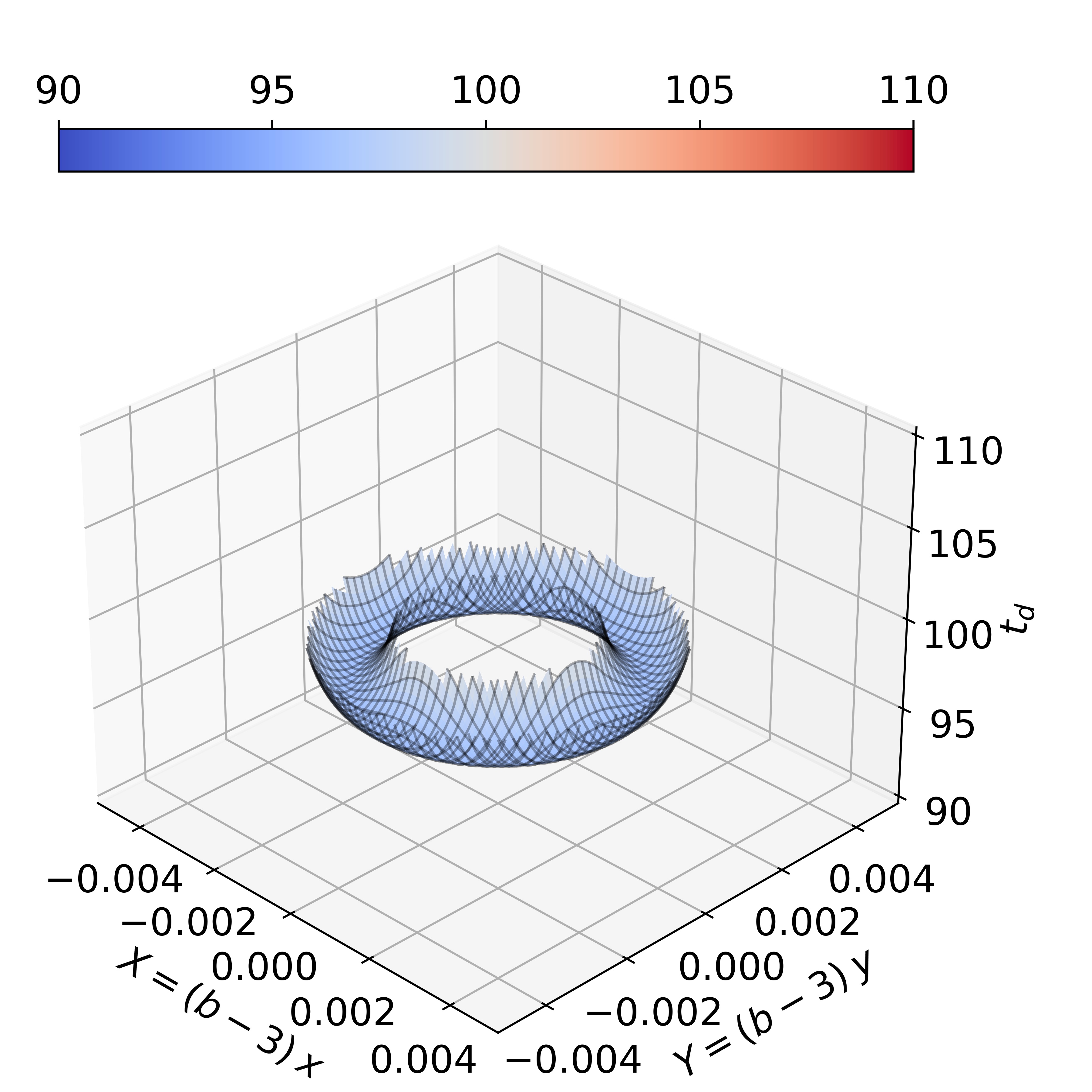
Figure 4: Time delay surface near primary/secondary/tertiary ring in the left/middle/right panel for axially symmetric case. The horizontal axes represent the spatial axes of the lens with respect to the observer (also equivalent to observer sky) and vertical axis represents the time delay values (in units of $GM/c^{3}$). In each panel, the $X$- and $Y$-axis have been transformed to remove the region inside the photon sphere.

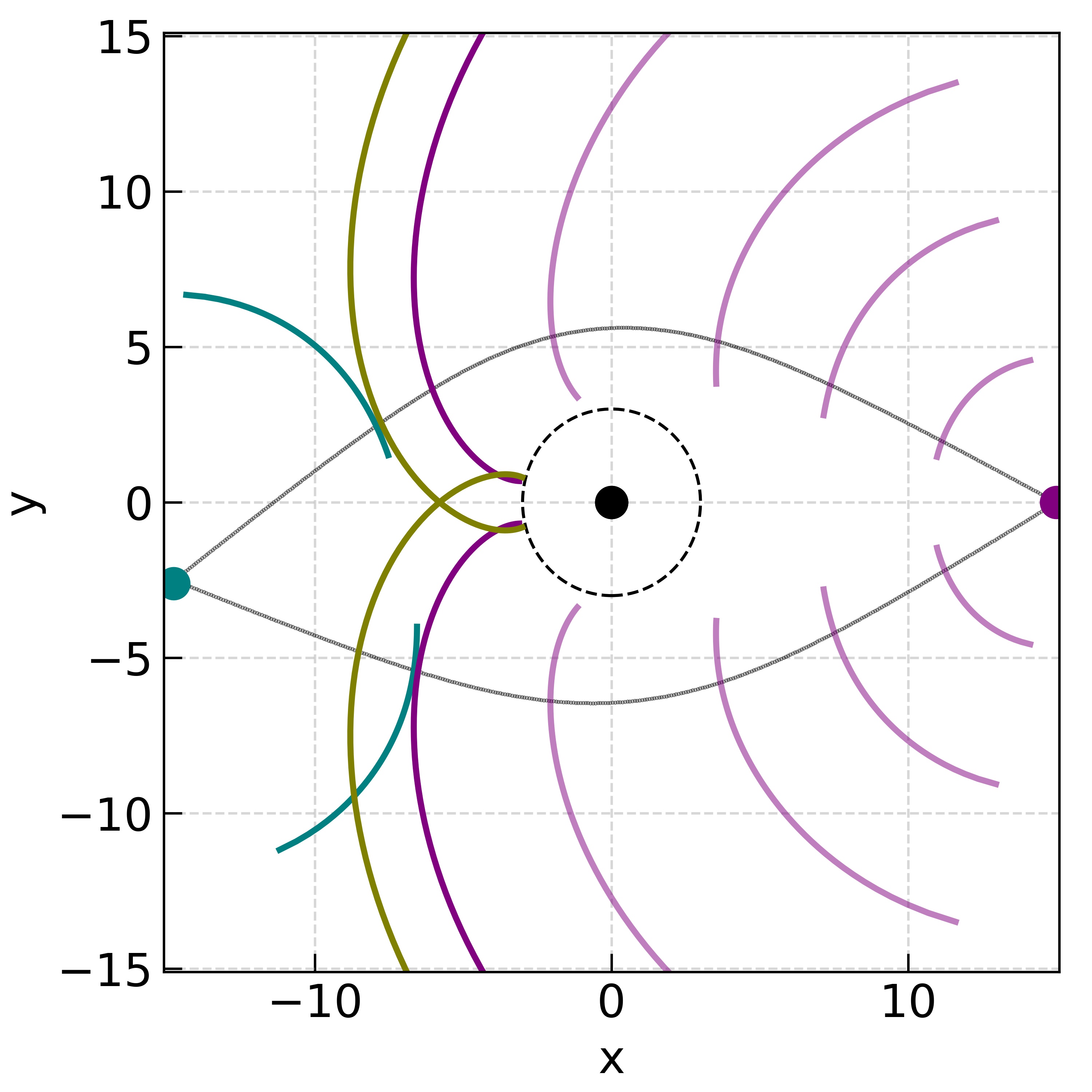
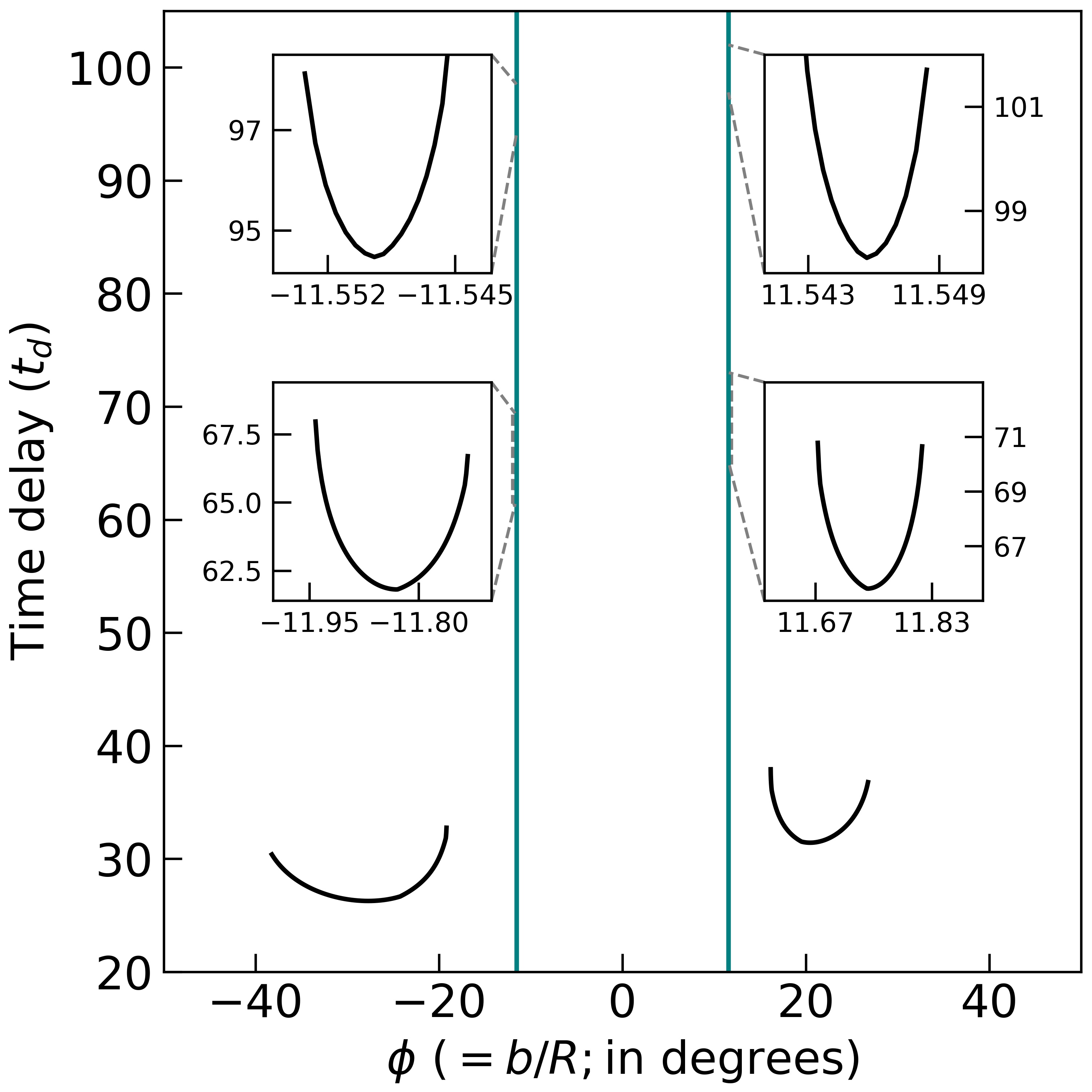
Figure 5: Wavefront propagation near a Schwarzschild black hole in the off-axis case. Left panel: The green, black and purple dots represent the position of the source, lens, and observer, respectively. The green curves represent the wavefront emitted by the source. The purple and olive curves represent a wavefront emitted from the observer at different time instances. The lensed images correspond to the points on purple/olive and green wavefronts where their normal vector agree with each other. These points are essentially the points in the figure where purple/olive and green wavefronts touch each other. The grey curves represent the corresponding rays emitted from the source and reach to the observer. Right panel: Time delay ($t_{d}$; in units of $GM/c^{3}$) as a function of angle of closest approach ($\phi$; in degrees) with respect to the observer for off-axis case. The green vertical lines mark the angle corresponding to the photon sphere. The black curves represent the slices of time delay surface near the primary, secondary, and tertiary images as we go from small to large time delays. For time delay surface near secondary and tertiary images, we show zoom-in plots since the images form very close to the photon sphere.

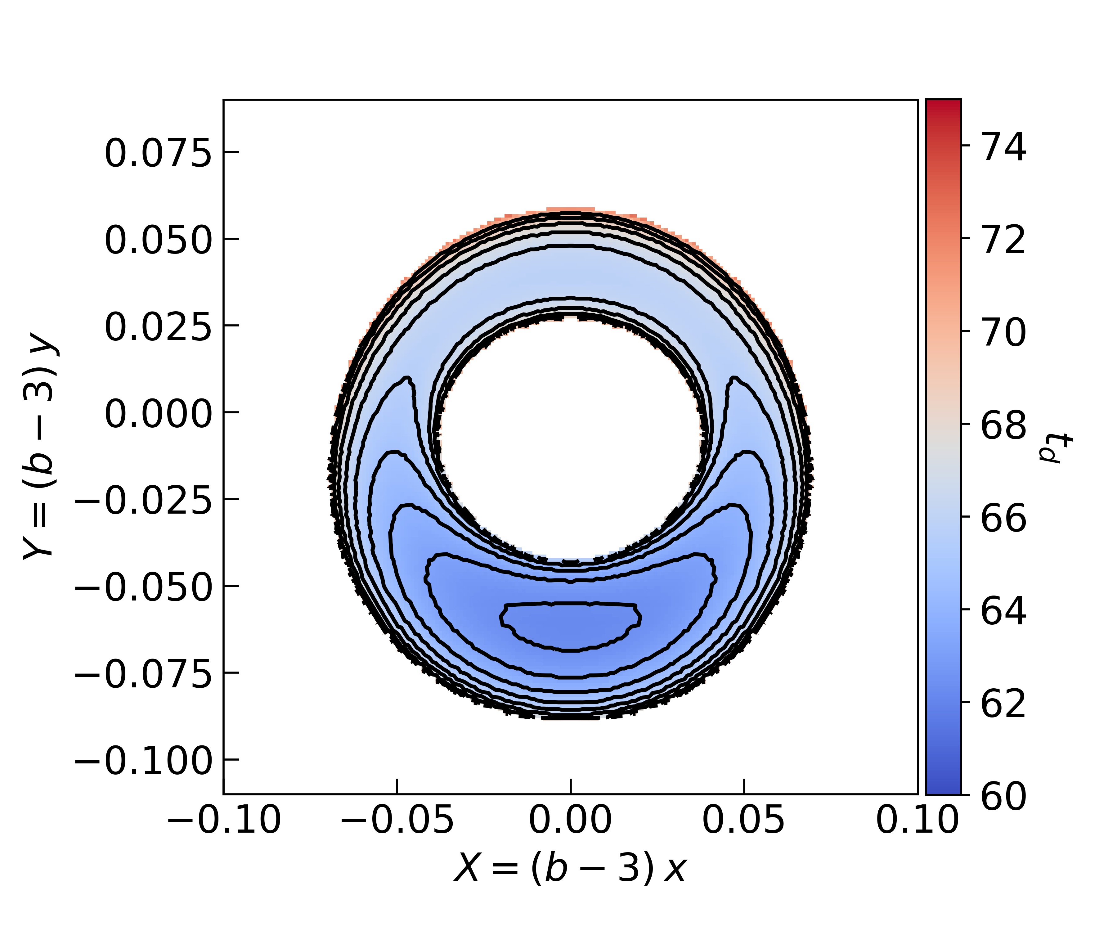
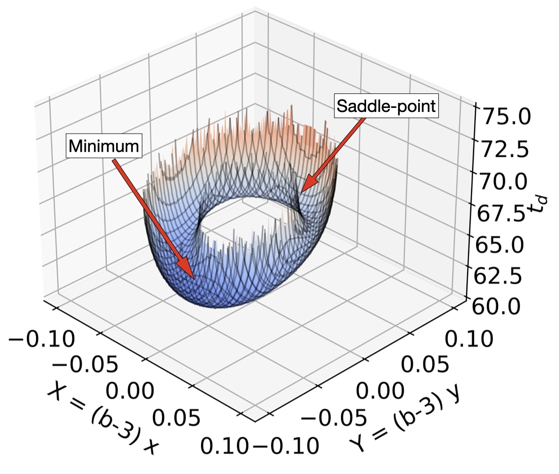
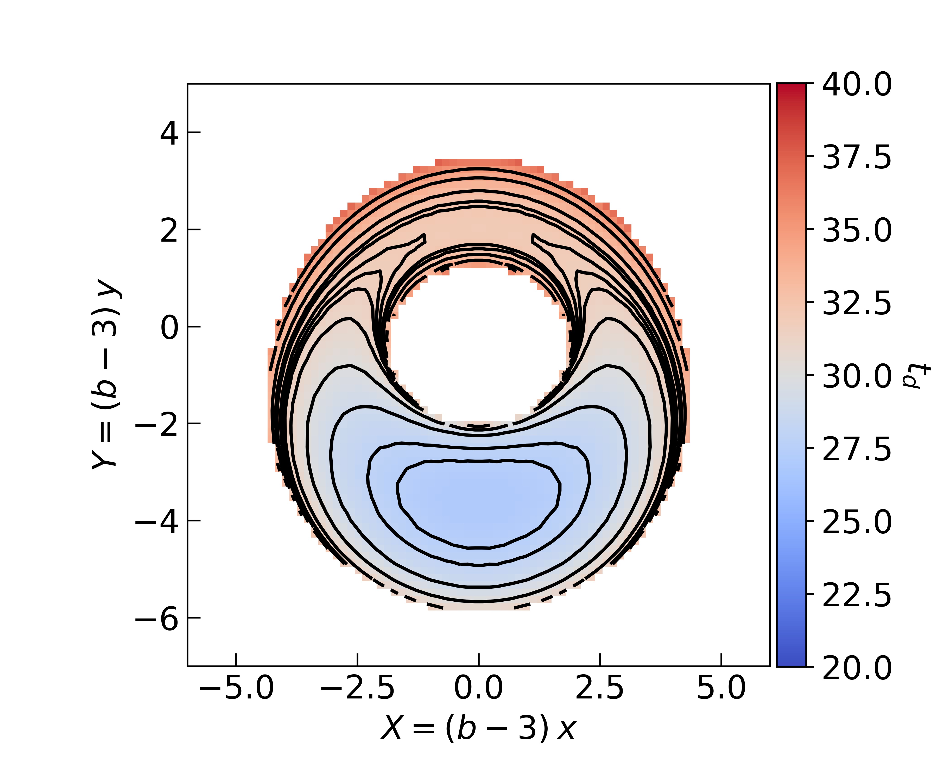
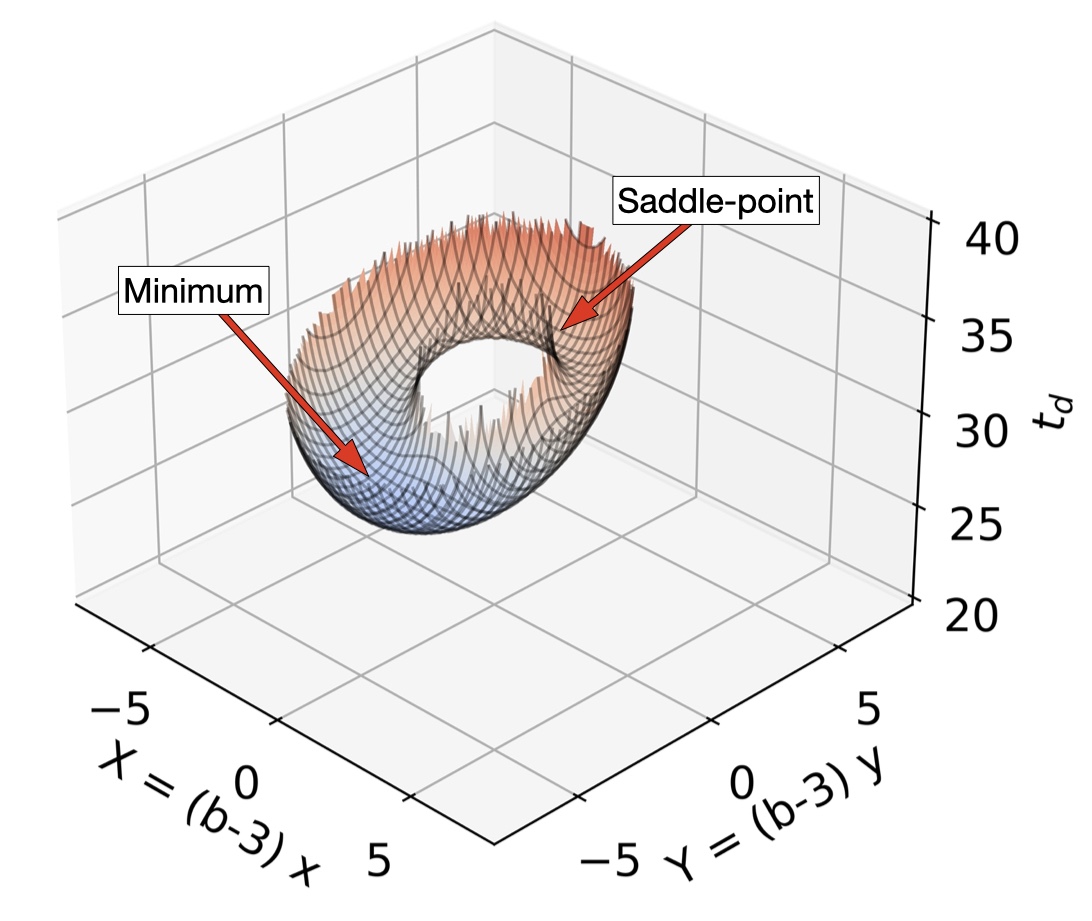
Figure 6: Time delay surface near primary and secondary image pairs for the off-axis case. The left column represents the time delay contours in 2D, whereas the right column represents the same plot in 3D. In the right column, red arrows mark the positions of minima and saddle-points on the 3D time delay surface. The bottom and top rows correspond to the primary and secondary image pairs respectively. In each panel, the X- and Y-axis are transformed to remove the region inside the photon sphere.

In our current work, to determine the path of light rays in the strong field and trace wavefronts originated from the source at $(t,r,\phi)=(0,R,\pi)$, we solve Equation (1) numerically while choosing a range of $b$ values. To numerically solve the coupled differential Equation (1), we use odeint from SciPy [49]. An example of light rays and wavefront propagation near the Schwarzschild black hole is shown in Figure 1. In each panel, the black dot represents the black hole, and the dashed circle around it marks the photon sphere ($r=3M$). The source is represented by the green dot and light rays emitted from the source are represented by the grey curves. The corresponding equal time surfaces (or wavefronts) for three different time values (in increasing order) are shown by green curves in the three panels from left to right. The break in the middle of the wavefront corresponds to the light rays which fall inside the black hole ($b<3M$). From Figure 1, we can see that the rays passing closer to the black hole are deflected more strongly compared to far away rays. Due to the large deflection close to the black hole, we observe part of the wavefront going around the black hole corresponding to the rays which loop around the black hole.

3 Axially symmetric case

In this section, we consider wavefronts for an axially symmetric configuration, i.e., the source, lens, and observer lie in a straight line (the optical axis).

To construct the time delay surface in our current work, we use forward and backward propagating wavefronts emitted by the source and observer, respectively, as described in [40; 41]. Figure 2 depicts the basic idea of using the wavefronts to locate the lensed image positions and construct the time delay surface. The green, black, and purple dots mark the positions of the source, black hole, and observer, respectively. We start by marking a forward propagating wavefront at a certain time as shown by the green curve. After that, we track a backward propagating wavefront emitted from the observer (shown by the purple curves at different times) and determine the time when it crosses the forward propagating wavefront. When purple and green wavefronts touch each other such that their normal vectors agree with each other, they correspond to the path of light rays emitted from the source and observed by the observer. This is further highlighted by the grey curves in Figure 2.

To indicate the crossing points of the forward and backward propagating wavefronts, we trace the individual rays corresponding to the backward wavefront as shown by purple and grey curves in the left panel of Figure 3. Grey (purple) curves mark the rays which (do not) cross the forward propagating wavefront. Whether a ray will cross the forward propagating wavefront or not will depends on the time at which we mark the forward propagating wavefront. In addition, the exact number of times a ray crosses the forward wavefront will also depend on the temporal position of the forward wavefront. If the forward wavefront is yet to cross the black hole, we can only get at most two crossings for a given ray. However, once it crosses the black hole, we can have many crossings (in principle) since a ray can loop around the black hole many times. We stop the forward wavefront before it crosses the black hole and only need the time corresponding to the first crossing for each ray.

For the axially symmetric case, time delay as a function of the emission direction $\phi$ for a given ray is shown in the right panel of Figure 3 (assuming $M=1$). The green vertical lines mark the $\phi$-values corresponding to the photon sphere ($r=3M$). Any photon emitted at an angle smaller than this will fall inside the black hole. The black U-shaped curves show the slices (at $y=0$) of a 3D time-delay surface near the primary, secondary, and tertiary images as we go from small to large time delay values. Since the secondary/tertiary images are formed when the light rays do one/two loops around the black hole, they form very close to the photon sphere, as can also be seen from the left panel. Due to the axial symmetry, in this case, we will observe (Einstein) ring formations for the primary/secondary/tertiary image, and all of these images are minima. In Figure 3, we also see that U-shaped curves for global minima seem to end around $\pm 40^{\circ}$ abruptly. Such a break is not physical and results from the fact that we do not have enough rays that can be used to determine the time delay surface at large angles. In principle, the curves will continue to go up (to infinity) as we go to larger angles.

This ring formation and parity of images can be seen clearly in the 3D plot of the time delay surface as shown in Figure 4. The $x$ and $y$ axes represent the spatial axes and $z$ axis shows the time delay values. The spatial axes are re-scaled such that $(X,Y)=(b-3)\left(x,y\right)$ to omit the $r<3M$ region. The left, middle, and right panels show the time delay surface near primary, secondary, and tertiary images, respectively. In each panel, the ring formation is obvious, as are the corresponding types of images (global minima for primary ring and local minima for secondary and tertiary rings).

From the right panel of Figure 3, we can see that the time delay surface near primary, secondary, and tertiary rings is not joined together, and there are gaps between them. This gap corresponds to rays that go behind the observer. A few such rays (in purple) can be seen in the left panel of Figure 3. Since the deflection will be continuous as we move closer to the black hole, there will always be a part of the forward wavefront between different order of images that will never reach the observer. We discuss this further in Section 5.

4 Off-axis case

The spherically symmetric nature of the Schwarzschild metric leads to the formation of rings when the source lies on the optical axis. However, once we move the source away from the optical axis, light rays emitted from the source and travelling from one side of the black hole will reach the observer earlier compared to the other side, and the ring formation will break into two separate images. Breaking of the Einstein ring into two distinct images can also be understood from the fact that light rays travel in constant $\theta$ planes around the Schwarzschild black hole due to its spherically symmetric nature. Hence, in the axis-symmetric case, there are infinite planes (for every $\theta$ value) containing the source, black hole, and observer such that a light ray emitted from the source can be observed by the source in any of these planes. Once we move the source away from the optical axis, there is only one plane that contains the source, black hole, and observer. Hence, light rays emitted from the source and travelling only in this plane can reach the observer. Within this plane, there are only two paths that connect the source and observer, leaving us with two images of the source. An example of this is shown in Figure 5. Here, we move the source (shown by a green dot) to a negative $y$ value. The forward (backward) propagating wavefront is shown in green (purple) color. We plot multiple temporal positions of the backward wavefront. The olive wavefront also shows the backward propagating wavefront at a larger time value than the purple colored wavefronts. Since we moved the source to the negative $y$ axis, the negative-$y$ part of the forward wavefront (lower half) will reach the observer first, implying that image on negative $\phi$ values will be observed first by the observer. This can also be seen from the fact that the lower half part of the green wavefront touches the last purple wavefront, whereas the upper half of the green wavefront touches the olive wavefront (which is drawn for a larger time). The light ray paths corresponding to the primary lensed images are shown by the grey curves. The breaking of ring in two different images can be more clearly seen in right panel of Figure 5 where we again plot time delay ($t_{d}$) as a function of angle of closest approach ($\phi$) for different rays as we observe that images formed on $\phi<0$ has smaller time delay values compared to the corresponding counterparts on $\phi>0$. Similar to Figure 4, we observe that the U-shaped curves corresponding to primary images abruptly end near $\pm 40^{\circ}$. Again, this is not physical and is a result of the fact that we do not have enough rays to draw the curves at these angles; otherwise, they would continue to go up to infinity. Another obvious yet important observation is the fact that in each (primary/secondary/tertiary) pair of lensed images, the image arriving later forms closer to the black hole.

Here, we can again ask for the parity of each of these images, but the $\phi-t_{d}$ plot shown in the left panel is not sufficient to determine the parity of these images since it only shows a 1D slice along $y$-axis of the full 3D time delay surface. Hence, we construct 2D as well as 3D time delay surface plots near the primary and secondary images, as shown in Figure 6. The 2D contour plots for primary and secondary images are shown in the bottom and top panel of the left column, respectively. The corresponding 3D plots are shown in the right column. From the left and right columns, we can clearly observe that the primary as well as secondary pair of images consist of one minima and one saddle-point. That said, it can be hard to locate the position of minima and saddle-points in the 3D plots (right panel), so we have explicitly pointed out their positions by red-coloured arrows. Due to the spherical symmetry of the lens, we expect to see the same image types even for higher-order images. To plot the time delay surface, we again use the same change of axes, $(X,Y)=(b-3)\left(x,y\right)$, and omit the $r<3M$ region. Similar to the axis-symmetric case, we again observe a gap in the time delay surface between primary and secondary images.

5 The “Home” and “Away” Images

In both of the above cases (axially symmetric and off-axis), we observed gaps in the time delay surface between each order of lensed images as seen from left panels in Figure 3 and 5. As mentioned briefly in Section 3, these gaps correspond to the part of the backward propagating wavefront that goes behind the observer and never crosses the forward wavefront. Or, from the forward wavefront perspective, part of the wavefront that loops around the black hole and goes behind the source itself. Since the deflection angle is continuously increasing as we move closer to the black hole, there will always be a part of the forward (backwards) propagating wavefront that will go behind the source (observer). We remark that in standard lensing theory, singular lenses such as a point mass, which do not explicitly invoke black holes, also have similar gaps in time delay surface, which can be considered as the infinitely time delayed maxima forming at the position of the point lens [e.g., 50] assuming that the time delay surface is continuous.

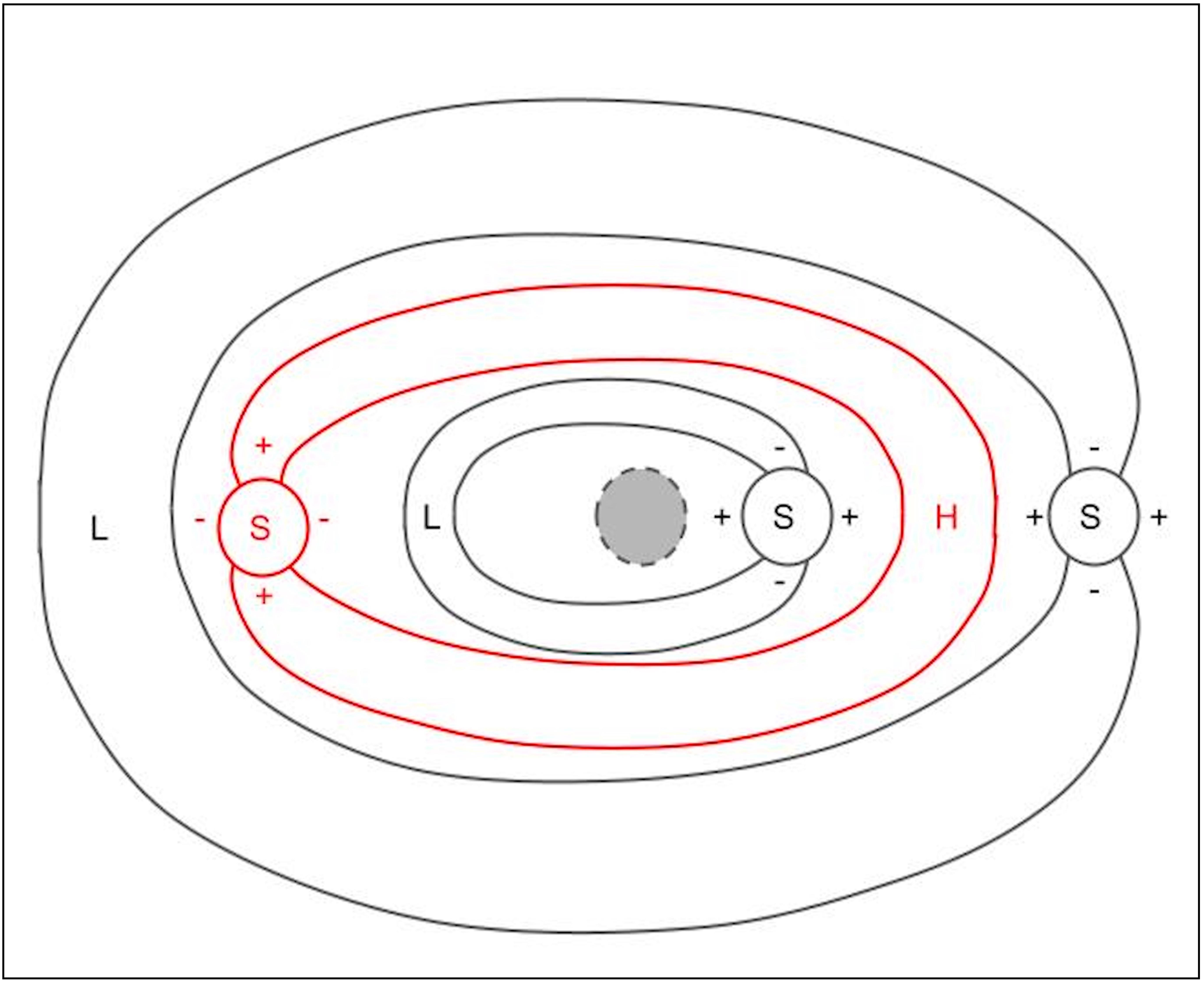
Figure 7: A schematic representation of the time-delay surface topology near a Schwarzschild black hole for the off-axis case[extending Figures 5.7 and 5.8 in ref. 11]. The position of the black hole is shown by the gray shaded region encircled by dashed curve at the centre of the plot. “L”, “S”, and “H” denote the position of minima, saddle-point, and maxima, respectively. The ‘+’ and ‘-’ signs around saddle-points indicate the directions in which time delay values are increasing and decreasing compared to time delay values at the saddle-points, respectively. The image positions in black, marks the position of observed images (or “home” images) where image positions in red mark the infinitely delayed images (or “away” images) which we expect to form in gaps between the home images. Here we only show the first two orders of home images and one set of away images, but the same topology is expected even for the higher-order images.

Near a Schwarzschild black hole, we can again ask the question, assuming that the time delay surface is continuous, do we expect additional images to form in these gaps between observed images? To answer this question, we need to determine the time delay surface topography near the black hole. A schematic surface is shown in Figure 7 for the off-axis case. The position of the black hole is shown by the grey shaded region inside the dashed circle. Here, the type of images are marked by “L”, “S”, and “H” for minima (or low), saddle-point, and maxima (or high), respectively. The black markers show what we may call “Home” image positions, i.e., images observed by the observer. On the left side of the black hole, we see the formation of two such minima, whereas on the right side, we see the formation of two such saddle-points. These correspond to the first two orders of images (primary and secondary) shown in Figure 6. In between these home minima (saddle-points), we show the formation of an infinitely delayed saddle-point (maxima) shown in red, which we call “Away” images since they never reach the observer. Although here we only show the topography near primary and secondary home images, we expect the same for further higher-order images due to the spherical symmetry of the lens. Since the proposed images in gaps are not observed, the above topology makes the time delay surface continuous. In addition, in the above topology, one (global) maxima will also form at the position of the black hole ($r<3M$). Doing so, in addition to making the time delay surface continuous, also satisfies the odd image theorem [51]. In addition, if we move the source also on the observer side (or observer on the source side) of the black hole by changing the sign of the x-coordinate, then the earlier home images become away images and earlier away images become home images.

6 Conclusions

The formation of multiple images through gravitational lensing is now a commonplace in astronomy and has a well-developed theoretical formalism to interpret the observables. This formalism assumes weak gravitational fields, and consequently small deflections, which do not apply to the multiple images formed near a black hole, such as observed near the M87 black hole. Can the existing formalism be generalised to these strong-field applications?

In this work we show that the key element of the weak-field formalism does generalise rather simply. This element is the abstract construction known variously as the time-delay surface, the arrival-time surface, or the Fermat potential. Lensed images form at the zero-gradient locations of the surface (maxima, minima, and saddle-points), and higher derivatives give various properties of images, such as the apparent handedness or parity. In the weak-field formalism, the time delay surface is conventionally given by the sum of two contributions, one geometrical and one gravitational, to the light travel time. In strong fields, it is not clear how to identify two such separate contributions. However, an alternative definition of the time-delay surface, as the difference between a forward and a backward wavefront, can be applied to any static spacetime. We compute the time-delay surface near a Schwarzschild black hole and study its properties.

Concretely, we use crossings of forward and backward propagating wavefronts from the source and observer, respectively, to construct the time delay surface and determine the image types. In the axially symmetric case (having the source, lens centre, and observer on the same line), we observe ring formation corresponding to a minimal valley on time delay surface for primary (1st order), secondary (2nd order), and tertiary (3rd order) images. Moving the source away from the optical axis causes the ring to break into two separate images, one minimum and one saddle-point. We again show this by constructing the time delay surface near the primary as well as secondary images. The pattern will continue since near a Schwarzschild black hole there is an infinite sequence of images with continuously decreasing magnification factors (see Appendix C) as we move towards higher order in the sequence.

In between each ring (or pair of lensed images), we find steeply rising walls in the time delay surface. These walls are a result of the fact that near the black hole light rays can loop around the black hole and between each order of images there will be a certain fraction of rays emitted from the source that will never reach the observer and go behind the source itself. Between a pair of walls we can think of two images, one saddle and one maximum, both infinitely delayed and therefore not visible. We name these away images, as distinct from the observable home images. A final image, infinitely demagnified and infinitely delayed, will form within the photon sphere ($r<3M$). The odd-image theorem remains valid. To an observer on the same side of the black hole as the source, home and away images get swapped, as do minima and maxima.

This work has been limited to a Schwarzschild black hole, for which we have mainly offered heuristic arguments from examining the numerical results on the time-delay surface. Formulating the image properties more precisely in terms of the surface is desirable, but it is not obvious how to proceed. The time-delay surface for a Kerr black hole, which would be more representative of the observations, would be interesting to compute, though significantly more complicated than the Schwarzschild case.

Appendix A Null geodesics in Schwarzschild spacetime

Lensing by a Schwarzschild black hole is a classical topic in the literature and there are several ways of computing light paths. One elegant approach is to treat $\frac{1}{2}g^{\mu\nu}p_{\mu}p_{\nu}$ as a Hamiltonian $(\mathcal{H})$ in four dimensions with canonical momentum $p_{\mu}\left(=\partial\mathcal{H}/\partial\dot{\mu}\right)$ being a new abstract vector and the affine parameter as the independent variable [e.g., 27].

The Schwarzschild metric itself is an exact static, spherically symmetric solution of Einstein’s field equations in vacuum[23]. Because of spherical symmetry, geodesics will be confined to a plane, and hence it is sufficient to consider the spacetime slice $(t,r,\phi)$. Omitting factors of $G$ and $c$ the metric can be written as

$$ds^{2}=-\left(1-\frac{2M}{r}\right)dt^{2}+\left(1-\frac{2M}{r}\right)^{-1}dr^{2}+r^{2}d\theta^{2}+r^{2}\sin^{2}\theta\>d\phi^{2},$$ (2)

where $M$ is the mass of the black hole. This metric leads us to

$$2\mathcal{H}=-\left(1-\frac{2M}{r}\right)^{-1}p_{t}^{2}+\left(1-\frac{2M}{r}\right)p_{r}^{2}+{p_{\phi}^{2}\over r^{2}},$$ (3)

with $\mathcal{H}=0$ for null geodesics (i.e., light rays). Solving Hamilton’s equations give

$$\dot{t} =-\left(1-\frac{2M}{r}\right)^{-1}p_{t},$$ (4)

$$\dot{r} =\left(1-\frac{2M}{r}\right)p_{r},$$

$$\dot{\phi} ={p_{\phi}\over r^{2}}.$$

We can derive the constants of motion using the equations,

$$\dot{p}_{t} =0\quad\Rightarrow\quad\left(1-\frac{2M}{r}\right)\dot{t}=E\>({\rm constant}),$$ (5)

$$\dot{p}_{\phi} =0\quad\Rightarrow\quad r^{2}\dot{\phi}=L\>({\rm constant}).$$

For light rays, $E$ and $L$ are equivalent to the energy and angular momentum of the ray. The constant value of $p_{t}\>(=E)$ is arbitrary, and we can choose it to be -1 by rescaling the affine parameter. There is a non-trivial equation for $p_{r}$, but since $\mathcal{H}=0$ for light rays, we can simply eliminate $p_{r}$ to get

$$\dot{r}=\sqrt{1-\frac{p_{\phi}^{2}}{r^{2}}\left(1-\frac{2M}{r}\right)}.$$ (6)

The square root implies $r\geq b$, where $r=b$ represents the closest approach, which is defined by

$$p_{\phi}^{2}={b^{3}\over b-2M}.$$ (7)

Putting $r=b$ is equivalent to setting $\dot{r}=0$ and $p_{r}=0$, which are the conditions that a circular orbit will have and leads to $r=3M$ (i.e., a photon sphere). With the above, Hamilton’s equations (4) now reduce to

$${dr\over dt} =\left(1-\frac{2M}{r}\right)\dot{r},$$ (8)

$${d\phi\over dt} =\left(1-\frac{2M}{r}\right){p_{\phi}\over r^{2}},$$

determining the trajectory of rays emitted by the source and passing near the black hole. Eq. (1) in the main text is simply Eqs. (6–8) collected together.

The differential equations (8) can be easily integrated numerically, starting from $r=b$ and any initial $\phi$. Some care is needed, however, because $dr/dt$ is not well-behaved at $r=b$. We can change variable to $w$, where

$$r=b+w^{2}\qquad$$ (9)

which transforms the $r$ equation to

$$\frac{dw}{dt}=\left(1-\frac{M}{b+w^{2}}\right)\frac{\dot{r}}{2w}$$ (10)

which is well-behaved at $w=0$ (that is, $r=b$) because

$$\frac{\dot{r}^{2}}{(2w)^{2}}=\frac{b-3}{2(b-2)}+O(w^{2})$$ (11)

This last quantity, it turns out, can actually be expressed as

$$\sum_{n=0}^{\infty}\left(\frac{-1}{b}\right)^{n+1}\frac{(n+2)(n+3-b)}{4(b-2)}\;v^{2n}$$ (12)

but only the $w\rightarrow 0$ limit is needed.

Appendix B Limiting cases

The above equations have three interesting limiting cases for different $b$ values,

1. $b\gg M$: This case corresponds to the weak field approximation. Even in the weak field regime, we have conventional terms like, “strong lensing” and “weak lensing”. In weak field limit, strong lensing refers to the case where we observe formation of multiple images.

2. $b\ll R$: we have a small lens, which behaves as a deflector of straight light paths.

3. $b\rightarrow 3M$: A photon does multiple orbits around the black hole before going away. If $b<3M$ the photon falls into the black hole.

The standard astrophysical scenario satisfies the first two limits, i.e., $R\gg b\gg M$. In such a case, to determine the total deflection angle, it is useful to write $\phi$ as a function of $r$,

$${d\phi\over dr}={1\over r^{2}}{1\over\sqrt{{b-2M\over b^{3}}-{r^{3}\over r-2M}}}.$$ (13)

The total deflection angle experienced by a light ray emitted from a source at $(r,\phi)=(R,\pi)$ is

$$\phi=\pi-2\int_{b}^{R}{dr\over r^{2}\sqrt{{b-2M\over b^{3}}-{r^{3}\over r-2M}}}.$$ (14)

Here, we introduce a change of variable, $u={R-r\over R-b}{b\over r}$ such that

$$\phi=\pi-2\int_{0}^{1}{du\over\sqrt{1-u^{2}-\frac{2M}{b}(1-u^{3})+\frac{2b}{R}(1-u)}}.$$ (15)

Binomial expansion to first order in $M/b$ and $b/R$ leads to

$$\phi=\pi-2\int_{0}^{1}{1\over\sqrt{1-u^{2}}}\left(1+{1+u+u^{2}\over 1+u}{M\over b}\right.\left.-{1\over 1+u}{b\over R}\right).$$ (16)

Solving the above integral after substituting $u=\cos w$ leads to,

$$\phi\simeq 2\frac{b}{R}-\frac{4M}{b},$$ (17)

which is essentially a straight line with an extra deflection of $4M/b$.

On the other hand, in the strong field limit ($b\rightarrow 3M$) with $R\rightarrow\infty$, we replace $b$ by $3M(1+\epsilon)$ and introduce a change of variable such that

$$r=3M\frac{1+\epsilon}{1-v}.$$ (18)

Since, in such a case, the integral in Equation (14) will be dominated by contribution near $v=0$, we have

$$\phi\simeq\pi+2\int_{0}^{1}\frac{dv}{\sqrt{v^{2}+\frac{2}{3}\epsilon}},$$ (19)

leading to

$$\phi\simeq 2\ln(\epsilon)+\dots$$ (20)

Appendix C Magnification

To calculate magnification, we need to set up a correspondence between lensed and unlensed rays. One could argue for different ways of doing so, but one reasonable definition for an unlensed ray is to require it to have the same value of $p_{\phi}$ as the lensed ray. The unlensed ray travels in a Euclidean line to some $\bar{\phi}$ (say). From the geometry it is easy to see that (i) the unlensed ray makes an angle ${\textstyle\frac{1}{2}}\bar{\phi}$ with the $x$ axis, and (ii) the closest approach of this ray to the origin is $R\sin{\textstyle\frac{1}{2}}\bar{\phi}$. Since for $M=0$ the closest approach is simply $p_{\phi}$ we have

$$\sin{\textstyle\frac{1}{2}}\bar{\phi}=\frac{p_{\phi}}{R}$$ (21)

In other words, the unlensed ray is a line from $(R,\pi)$ to $(R,R\bar{\phi})$, where $\bar{\phi}$ is given by (21). The derivative $\mathchoice{\partial{\bar{\phi}}\over\partial{\phi}}{\partial{\bar{\phi}}/\partial{\phi}}{\partial{\bar{\phi}}/\partial{\phi}}{\partial{\bar{\phi}}/\partial{\phi}}$ is a possible definition of magnification in the $\phi$ direction.

More interesting, however, is the ratio of lensed and unlensed solid angles, since it corresponds to light flux. Going to three dimensions, and considering the solid angles within $\phi$ and $\bar{\phi}$ we have

$$\Omega=4\pi\,\sin^{2}\!{\textstyle\frac{1}{2}}\phi\qquad\bar{\Omega}=4\pi\,\frac{p_{\phi}^{2}}{R^{2}}$$ (22)

The solid-angle magnification (sometimes called amplification) is

$$A\equiv\mathchoice{\partial{\bar{\Omega}}\over\partial{\Omega}}{\partial{\bar{\Omega}}/\partial{\Omega}}{\partial{\bar{\Omega}}/\partial{\Omega}}{\partial{\bar{\Omega}}/\partial{\Omega}}=\frac{4}{R^{2}}\,\frac{p_{\phi}}{\sin\phi}\,\mathchoice{d{p_{\phi}}\over d{\phi}}{d{p_{\phi}}/d{\phi}}{d{p_{\phi}}/d{\phi}}{d{p_{\phi}}/d{\phi}}$$ (23)

The amplification becomes singular at $\phi=0$. The regime of $|\bar{\phi}|$ small and $|\phi|$ large corresponds to strong-field lensing. The curve is nearly flat, indicating very faint images, but there are tiny step-like features at multiples of $180^{\circ}$. The regime $|\phi|$ large and $\bar{\phi}\simeq\phi$ is where the light is always far from the lens. Here the slope is close to unity — but must be slightly less than unity to compensate for the steep regions.

Let us now consider limiting forms of the amplification (23).

For the most-deflected part of the wavefront, we take the $b\rightarrow 3M$ limit, corresponding to Eq. (20). This gives

$$A=\frac{\epsilon}{R^{2}\sin\phi}\;\mathchoice{d{p_{\phi}^{2}}\over d{\epsilon}}{d{p_{\phi}^{2}}/d{\epsilon}}{d{p_{\phi}^{2}}/d{\epsilon}}{d{p_{\phi}^{2}}/d{\epsilon}}\propto{e^{-|\phi|}\over\sin\phi}$$ (24)

Thus, the flux in the later images falls off quickly.

For small angles, we have

$$A=\frac{\bar{\phi}}{\phi}\;\mathchoice{d{\bar{\phi}}\over d{\phi}}{d{\bar{\phi}}/d{\phi}}{d{\bar{\phi}}/d{\phi}}{d{\bar{\phi}}/d{\phi}}$$ (25)

From the lens equation (17) we have

$$\phi=\bar{\phi}-(2\phi_{E})/\bar{\phi}$$ (26)

where we have defined

$$\phi_{E}\equiv\frac{2M}{R}$$ (27)

the conventionally definition of the Einstein radius for the case of observer-lens and lens-source distances both equal to $R$. For the flux we get

$$A=\left(1-(2\phi_{E}/\bar{\phi})^{4}\right)^{-1}$$ (28)

Now, from the form of (26) it is clear that there will be two values of $\bar{\phi}$, one each greater and less in magnitude than $2\phi_{E}$. Hence, for small angles, there is always one image with amplification greater than unity. This is the flux-conservation paradox. Its resolution depends on precisely how the amplification is defined — recall that the definition (21) is not unique — but basically, the answer is that at large angles the amplification dips very slightly below unity[54].

References

- Einstein [1911] A. Einstein, Annalen der Physik 340, 898 (1911).
- Einstein [1916] A. Einstein, Annalen der Physik 354, 769 (1916).
- Einstein [1936] A. Einstein, Science 84, 506 (1936).
- Dyson et al. [1920] F. W. Dyson, A. S. Eddington, and C. Davidson, Philosophical Transactions of the Royal Society of London Series A 220, 291 (1920).
- Walsh et al. [1979] D. Walsh, R. F. Carswell, and R. J. Weymann, Nature 279, 381 (1979).
- Lynds and Petrosian [1986] R. Lynds and V. Petrosian, in Bulletin of the American Astronomical Society, Vol. 18 (1986) p. 1014.
- Soucail et al. [1987] G. Soucail, B. Fort, Y. Mellier, and J. P. Picat, A&A 172, L14 (1987).
- Blandford and Narayan [1992] R. D. Blandford and R. Narayan, ARAA 30, 311 (1992).
- Bartelmann [2010] M. Bartelmann, Classical and Quantum Gravity 27, 233001 (2010), arXiv:1010.3829 [astro-ph.CO] .
- Perlick [2010] V. Perlick, arXiv e-prints , arXiv:1010.3416 (2010), arXiv:1010.3416 [gr-qc] .
- Schneider et al. [1992] P. Schneider, J. Ehlers, and E. E. Falco, Gravitational Lenses (1992).
- Corral-Santana et al. [2016] J. M. Corral-Santana, J. Casares, T. Muñoz-Darias, F. E. Bauer, I. G. Martínez-Pais, and D. M. Russell, A&A 587, A61 (2016), arXiv:1510.08869 [astro-ph.HE] .
- Abbott et al. [2016] B. P. Abbott et al., Phys Rev D 93, 122003 (2016), arXiv:1602.03839 [gr-qc] .
- Abbott et al. [2018] B. P. Abbott et al., Phys. Rev. Lett. 121, 161101 (2018), arXiv:1805.11581 [gr-qc] .
- Sahu et al. [2022] K. C. Sahu et al., ApJ 933, 83 (2022), arXiv:2201.13296 [astro-ph.SR] .
- Collaboration [2019a] E. H. T. Collaboration, ApJL 875, L1 (2019a).
- Collaboration [2019b] E. H. T. Collaboration, ApJL 875, L2 (2019b).
- Collaboration [2019c] E. H. T. Collaboration, ApJL 875, L3 (2019c).
- Collaboration [2019d] E. H. T. Collaboration, ApJL 875, L4 (2019d).
- Collaboration [2022a] E. H. T. Collaboration, ApJL 930, L12 (2022a).
- Collaboration [2022b] E. H. T. Collaboration, ApJL 930, L13 (2022b).
- Collaboration [2022c] E. H. T. Collaboration, ApJL 930, L14 (2022c).
- Schwarzschild [1916] K. Schwarzschild, Sitzungsberichte der Königlich Preussischen Akademie der Wissenschaften , 189 (1916).
- Schwarzschild [1999] K. Schwarzschild, arXiv e-prints , physics/9905030 (1999), arXiv:physics/9905030 [physics.hist-ph] .
- Darwin [1959] C. Darwin, Royal Society of London Proceedings Series A 249, 180 (1959).
- Ohanian [1987] H. Ohanian, AJP 55, 428 (1987).
- Chandrasekhar [1983] S. Chandrasekhar, The mathematical theory of black holes (Oxford/New York, Clarendon Press/Oxford University Press (International Series of Monographs on Physics. Volume 69), 663 p., 1983).
- Virbhadra and Ellis [2000] K. S. Virbhadra and G. F. R. Ellis, Phys Rev D 62, 084003 (2000), arXiv:astro-ph/9904193 [astro-ph] .
- Bozza et al. [2001] V. Bozza, S. Capozziello, G. Iovane, and G. Scarpetta, General Relativity and Gravitation 33, 1535 (2001), arXiv:gr-qc/0102068 [gr-qc] .
- Frittelli et al. [2000] S. Frittelli, T. P. Kling, and E. T. Newman, Phys Rev D 61, 064021 (2000), arXiv:gr-qc/0001037 [gr-qc] .
- Bozza [2002] V. Bozza, Phys Rev D 66, 103001 (2002), arXiv:gr-qc/0208075 [gr-qc] .
- Bozza [2003] V. Bozza, Phys Rev D 67, 103006 (2003), arXiv:gr-qc/0210109 [gr-qc] .
- Aazami et al. [2011] A. B. Aazami, C. R. Keeton, and A. O. Petters, Journal of Mathematical Physics 52, 092502 (2011), arXiv:1102.4300 [astro-ph.CO] .
- Gralla and Lupsasca [2020] S. E. Gralla and A. Lupsasca, Phys Rev D 101, 044031 (2020), arXiv:1910.12873 [gr-qc] .
- Hsieh et al. [2021] T. Hsieh, D.-S. Lee, and C.-Y. Lin, Phys Rev D 103, 104063 (2021), arXiv:2101.09008 [gr-qc] .
- Refsdal [1964a] S. Refsdal, MNRAS 128, 295 (1964a).
- Refsdal [1964b] S. Refsdal, MNRAS 128, 307 (1964b).
- Refsdal [1966] S. Refsdal, MNRAS 132, 101 (1966).
- Frittelli and Petters [2002] S. Frittelli and A. O. Petters, Journal of Mathematical Physics 43, 5578 (2002), arXiv:astro-ph/0208135 [astro-ph] .
- Nityananda [1990a] R. Nityananda, Current Science 59, 1044 (1990a).
- Nityananda [1990b] R. Nityananda, in Gravitational Lensing, edited by Y. Mellier, B. Fort, and G. Soucail (Springer Berlin Heidelberg, Berlin, Heidelberg, 1990) pp. 1–12.
- Rauch and Blandford [1994] K. P. Rauch and R. D. Blandford, ApJ 421, 46 (1994).
- Frutos-Alfaro [2012] F. Frutos-Alfaro, Journal of Modern Physics 3, 1882 (2012), arXiv:1412.8068 [gr-qc] .
- Yang and Casals [2014] H. Yang and M. Casals, Phys Rev D 90, 023014 (2014), arXiv:1404.0722 [gr-qc] .
- Kling et al. [2019] T. P. Kling, E. Grotzke, K. Roebuck, and H. Waite, General Relativity and Gravitation 51, 32 (2019).
- Kling et al. [2018] T. P. Kling, K. Roebuck, and E. Grotzke, General Relativity and Gravitation 50, 7 (2018).
- Blandford and Narayan [1986] R. Blandford and R. Narayan, ApJ 310, 568 (1986).
- Nityananda and Samuel [1992] R. Nityananda and J. Samuel, Phys Rev D 45, 3862 (1992).
- Virtanen et al. [2020] P. Virtanen et al., Nature Methods 17, 261 (2020).
- Mollerach and Roulet [2002] S. Mollerach and E. Roulet, Gravitational Lensing and Microlensing (2002).
- Burke [1981] W. L. Burke, ApJL 244, L1 (1981).
- Harris et al. [2020] C. R. Harris et al., Nature 585, 357 (2020), arXiv:2006.10256 [cs.MS] .
- Hunter [2007] J. D. Hunter, Computing in Science and Engineering 9, 90 (2007).
- Wucknitz [2008] O. Wucknitz, MNRAS 386, 230 (2008), arXiv:0801.3758 .