Classification of dynamical Lie algebras for translation-invariant 2-local spin systems in one dimension

Abstract

Much is understood about $1$-dimensional spin chains in terms of entanglement properties, physical phases, and integrability. However, the Lie algebraic properties of the Hamiltonians describing these systems remain largely unexplored. In this work, we provide a classification of all Lie algebras generated by translation-invariant $2$-local spin chain Hamiltonians, or so-called dynamical Lie algebras. We consider chains with open and periodic boundary conditions and find $17$ unique dynamical Lie algebras. Our classification covers some well-known models such as the transverse-field Ising model and the Heisenberg chain, and we also find more exotic classes of Hamiltonians that cannot be identified easily. In addition to the closed and open spin chains, we consider systems with a fully connected topology, which may be relevant for quantum machine learning approaches. We discuss the practical implications of our work in the context of quantum control, variational quantum computing, and the spin chain literature.

I Introduction

Mathematical classifications of the fundamental symmetries of physical systems date back to the work of Wigner, who proposed three symmetry classes of non-interacting fermionic Hamiltonians depending on their time-reversal and spin-rotation properties [1]. Three decades later Dyson would mathematically solidify this theory and connect the spectral properties of these different types of Hamiltonians with random matrix theory [2] (see [3] for a modern treatment). It would take another thirty years before Altland and Zinbauer extended these results to ten symmetry classes [4], each of which correspond to a symmetric space in Cartan’s original classification of these spaces [5, 6]. Further extensions of these results were made in recent years with regards to topological phases of matter [7, 8, 9].

The above mathematical classifications of quantum physics rest on the powerful theory of Lie groups, which provides a framework for describing the continuous symmetries and transformations that characterize the behavior of quantum systems. The study of Lie groups, and by extension physical symmetries, can often be simplified by considering the corresponding Lie algebra of the group. The commutation relations of operators in the Lie algebra capture the essential features of the underlying symmetries and can be used to analyze the spectrum, eigenstates, and dynamics of quantum systems.

A Hamiltonian of a finite-dimensional system can be understood as ($i$ times) an element of some Lie algebra $\mathfrak{g}\subseteq\mathfrak{su}(N)$. Here, $\mathfrak{su}(N)$ is the vector space of all skew-Hermitian $N\times N$ matrices equipped with the standard commutator. Typically, a Hamiltonian is described by a linear combination of terms that correspond to a certain physical interaction. These individual terms can be used to generate a Lie algebra, which is called the Hamiltonian algebra or dynamical Lie algebra (DLA) [10, 11, 12, 13, 14], which is intricately linked to the dynamics of quantum systems.

Since each DLA is a subalgebra of $\mathfrak{su}(N)$, a classification of DLAs can be phrased as a classification of all subalgebras of $\mathfrak{su}(N)$. Such a classification is intractable, except when specific constraints are placed on the subalgebras one considers. For example, in the original works of Killing and Cartan, all simple Lie algebras were classified [15]; similarly, Dynkin provided a classification of the maximal subalgebras of simple Lie algebras [16, 17]. We follow a different approach: instead of adding algebraic constraints such as simplicity or maximality, we make use of the fact that any Lie algebra can be described by a set of generators, and we consider the Lie algebras that arise by using the terms of specific Hamiltonians as the generators. In contrast with the previously-mentioned classifications of [1, 2, 4], this approach contains interacting quantum many-body systems.

Specifically, we consider the class of Hamiltonians that correspond to $1$-dimensional $2$-local spin chains, and provide a classification of the Lie algebras that are generated under commutation by the terms of the Hamiltonian. Much about these systems is well-understood, from their entanglement properties [18], their phases [19] and their integrability [20, 21]. However, to the best of our knowledge, the Lie algebraic properties of these Hamiltonians have not yet been explored in full. It is thus reasonable to ask, given our comprehensive knowledge of the physics governing these systems, what more can be learned from the Lie algebra? In short, our classification has bearing on areas of quantum control, variational quantum computing, and quantum dynamics and thermodynamics.

In quantum control, the DLA of a dynamical quantum system can be related to the set of reachable states of that system. In particular, DLAs can be used to define a notion of controllability of a quantum system [22, 23, 24], which is highly relevant when it comes to designing unitary operations for quantum simulators and quantum computers. One is typically interested in Hamiltonians that can generate an arbitrary unitary operator, while the existence of symmetries can inhibit the control of a physical system [25].

For variational quantum computing, one is not interested in representing the whole unitary group, but in using a parameterized subgroup in order to generate a state that maximizes a given objective function. Understanding what subgroup a particular quantum circuit parameterizes can give insight into its representational power. For example, one can connect the dimension of the DLA to a phenomenon called overparameterization [26, 27, 28, 29]. Additionally, DLAs can be used to understand barren plateaus [30] — flat areas in the cost landscape of a variational quantum algorithm that hinder optimization [31, 32]. Finally, a recent work uses knowledge of the DLA to perform efficient classical simulations of several quantum algorithms [33].

Finally, one can use the knowledge of the DLA to provide insights into the dynamics and thermodynamics. For example, one can construct constant-depth quantum circuits for the dynamical simulation of a specific quantum system [34, 35, 36, 37], or state preparation via adiabatic state preparation [35, 37], or implement Hartree–Fock [38]. The dimension of the DLA is directly related to the quantum circuit depth needed to capture the full dynamics [34]. Thermodynamic properties are in part encoded in the commutant of the DLA, i.e., in the conserved charges [39]. Non-Abelian commutants lead to non-trivial quantum effects in thermodynamics, which affects thermalization properties among others.

The paper is structured as follows. We end the introduction with a summary of our main mathematical results. Then, in Sect. II, we establish our notation and introduce the necessary mathematical preliminaries. We discuss the method of our classification in Sect. III and present the main results in Sect. IV. Finally, we discuss the implications of our results in Sect. V. In the Supplemental Materials (abbreviated SM), we first review preliminaries on Pauli strings and Lie algebras and then present the full details of the proofs of the main results.

I.1 Summary of the main results

Here, we give a brief summary of our main results, which include the classification of all DLAs generated by 2-local spin Hamiltonians of length $n$ in one dimension. Recall that a Lie algebra can be constructed by a set of generators so that it is closed under linear combinations and under the Lie bracket. In our case, the Lie bracket is the standard commutator $[A,B]=AB-BA$. We now choose the generators of our Lie algebra to be ($i$ times) the terms of any 2-local spin chain Hamiltonian. Since a Hamiltonian is always a Hermitian operator, we can understand it as ($i$ times) an element of the Lie algebra $\mathfrak{u}(2^{n})$. Therefore, we can limit ourselves to the study of DLAs that are subalgebras of $\mathfrak{u}(2^{n})$, for which we have the following useful fact. Although this result is known (see e.g. [25, 40]), for completeness, we provide its proof and review the necessary definitions in SM II.

Proposition I.1.

A DLA must be either Abelian, $\mathfrak{su}(N^{\prime})$, $\mathfrak{so}(N^{\prime})$, $\mathfrak{sp}(N^{\prime\prime})$ $($with $N^{\prime}\leq 2^{n}$, $N^{\prime\prime}\leq 2^{n-1})$, an exceptional compact simple Lie algebra, or a direct sum of such Lie algebras. Indeed, any subalgebra of $\mathfrak{u}(N)$ is either Abelian or a direct sum of compact simple Lie algebras and a center.

Note that all simple Lie algebras over the complex and real numbers have been classified by Killing and Cartan [41]. The above proposition forms the backbone of our classification, as we know that any DLA generated by our class of Hamiltonians must be of the described form.

To obtain the classification, we first calculate all DLAs of the power set of Hamiltonians for a $2$-site system, and identify the unique sets of generators. Then we identify the orbits under the symmetries of the Pauli group and the swap of the two sites, thus reducing the number of unique Lie algebras to $27$. Next, we find several isomorphisms between some of the sets of generators, reducing the set of unique structures even further. Finally, we determine how these Lie algebras scale with system size as the number of spins grows beyond $2$ sites. In this final step, we take the topology of the spin chain into account, since the Lie algebra will behave differently for open or periodic boundary conditions of the chain. The following is our main result.

Result I.1 (Classification of spin chain DLAs).

We provide a classification of all dynamical Lie algebras of $2$-local spin Hamiltonians in one dimension. For both open and closed spin chains, there are $17$ unique Lie algebras that can be generated by a spin chain Hamiltonian.

The formal statement of this result is presented in the main text with Theorems IV.1 and IV.2 along with a sketch of the proof. The dimension of a DLA can be related to the trainability of variational quantum circuits, and may therefore be of high interest. Since we know the dimensions of all simple Lie algebras, a direct corollary of our result is the following.

Result I.2 (Dimension scaling of DLAs).

The dimension of any dynamical Lie algebra of a $2$-local spin chain Hamiltonian of length $n$ will scale as either $O(4^{n})$, $O(n^{2})$ or $O(n)$.

To illustrate this, we plot the dimensions of the open DLAs in our classification in Figure 1.

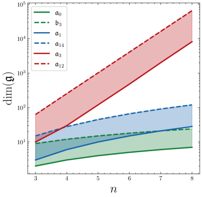
Figure 1: Scaling of the DLAs of spin chains with open boundary conditions. The exponentially scaling DLAs are denoted in red, the quadratically scaling ones in blue, and the linearly scaling algebras are denoted in green. The full and dashed line denote the smallest and largest scaling algebra in our classification, respectively.

Our proof technique also applies to the case of a permutation-invariant graph, where each site is interacting with every other site via at most 2-local interactions; in other words, all-to-all connected. We therefore also include this topology in our classification.

Result I.3 (Classification of permutation invariant DLAs).

We provide a classification of all dynamical Lie algebras of $2$-local permutation-invariant spin Hamiltonians. There are $8$ unique Lie algebras that can be generated by such a spin chain Hamiltonian.

We present the formal statement of this result in Theorem IV.3. Similarly to Result I.2, we find DLAs with linear, quadratic and exponentially scaling dimensions.

In addition to the classification of unique Lie algebraic structures, we also provide an explicit list of Hamiltonians that generate them in Table S.I. Some of the models in our classification correspond to well-known models such as the transverse-field Ising model or the Heisenberg model, whereas other Hamiltonians are perhaps not realizable in nature. However, some of these more exotic models may be of interest due to their properties. For instance, we find a class of Hamiltonians with globally non-commuting charges, which are known to be of interest in quantum thermodynamics [39, 42].

II Background

II.1 Glossary

We summarize the main choices of notation and nomenclature used throughout the paper in the following list.

• Lie algebras.

• Sets, usually generating sets for Lie algebras.

• The Lie algebra generated by a set $\mathcal{G}$.

• $\mathfrak{a}$ and $\mathfrak{b}$ are isomorphic as Lie algebras.

• $\mathcal{A}$ and $\mathcal{B}$ are equivalent under the symmetry group $S_{3}\times\mathbb{Z}_{2}$ .

• $\mathcal{A}$ and $\mathcal{B}$ are equal as sets.

• The set of $n$-qubit Pauli strings $\{I,X,Y,Z\}^{\otimes n}$.

• The action of the corresponding Pauli matrix on the $j$-th qubit in the spin chain.

• The set of all linear combinations of elements of $\mathcal{A}$ with real coefficients.

• A shortcut for taking the real span and multiplying by the imaginary unit $i$. Takes Hermitian matrices to skew-Hermitian.

II.2 Preliminaries

We assume knowledge of finite-dimensional Lie algebras (for a formal treatment, see e.g. Refs. [6, 41]), but will review some essential concepts here. A Lie algebra $\mathfrak{g}$ is a vector space equipped with a Lie bracket $[\cdot,\cdot]\colon\mathfrak{g}\times\mathfrak{g}\to\mathfrak{g}$ satisfying certain axioms (which are reviewed in SM II). The Lie bracket defines the adjoint endomorphism $\mathrm{ad}_{a}\colon\mathfrak{g}\to\mathfrak{g}$ where $\mathrm{ad}_{a}(b)=[a,b]$. For our purposes, the Lie bracket is the standard commutator of linear operators on a complex vector space: $[a,b]=ab-ba$. Due to the Lie-correspondence, we can associate a Lie group $G$ with a Lie algebra $\mathfrak{g}$ via the exponential map $G=e^{\mathfrak{g}}$.

Consider a set of generators $\mathcal{A}=\{a_{1},a_{2},\ldots,a_{M}\}$ with $a_{k}\in\mathfrak{g}$. We first define the nested commutator,

$$\mathrm{ad}_{a_{i_{1}}}\cdots\mathrm{ad}_{a_{i_{r}}}(a_{j})=[a_{i_{1}},[a_{i_{2}},[\cdots[a_{i_{r}},a_{j}]\cdots]]],$$ (1)

which is just $a_{j}$ in the special case $r=0$. The linear span of all nested commutators

$$\langle\mathcal{A}\rangle_{\mathrm{Lie}}:=\mathrm{span}\bigl{\{}\mathrm{ad}_{a_{i_{1}}}\cdots\mathrm{ad}_{a_{i_{r}}}(a_{j})\,\big{|}\,a_{i_{1}},\dots,a_{i_{r}},a_{j}\in\mathcal{A}\bigr{\}}$$

is then called a dynamical Lie algebra (DLA) [40, 10]. This is the minimal (under inclusion) subalgebra of $\mathfrak{g}$ that contains the set $\mathcal{A}$. The depth $r$ of the nested commutator is finite and will depend on the size of the DLA, which we typically do not know beforehand. In practice, the DLA of a given set of generators $\mathcal{A}$ can be obtained recursively with Algorithm 1.

Input: Set of generators $\mathcal{A}$

for $a_{i}\in\mathcal{A}$ do

       for $a_{j}\in\mathcal{A}$ do

             $a_{k}=[a_{i},a_{j}]$

             if $a_{k}\notin\mathcal{A}$ and $a_{k}\neq 0$ then

                   $\mathcal{A}\leftarrow\mathcal{A}\cup\{a_{k}\}$

                  

            

       end for

      

end for

$\langle\mathcal{A}\rangle_{\mathrm{Lie}}\leftarrow\mathrm{span}\{\mathcal{A}\}$

Algorithm 1 Calculating the DLA

II.3 Translation-invariant 2-local spin systems in one dimension

Due to Proposition I.1, we know what form the subalgebras of $\mathfrak{su}(N)$ must take. Our goal is to find which of these direct sums of simple or Abelian Lie algebras can be generated by a physically inspired set of generators.

In particular, we are interested in the subalgebras of $\mathfrak{su}(2^{n})$ that are generated by the terms of $1$-dimensional $2$-local Hamiltonians with translation-invariant structure, i.e., the type of the interactions between qubits is the same, but interaction strength may vary. We consider a spin system with a complex Hilbert space $(\mathbb{C}{{}^{2}})^{\otimes n}$ and a Hamiltonian $H$, which is a Hermitian operator on $(\mathbb{C}{{}^{2}})^{\otimes n}$ of the form

$$H=\sum_{k=1}^{n-1}\sum_{a\otimes a^{\prime}\in\mathcal{A}}a_{k}\otimes a^{\prime}_{k+1},$$ (2)

where

$$a_{k}\otimes a^{\prime}_{k+1} :=I^{\otimes(k-1)}\otimes a\otimes a^{\prime}\otimes I^{\otimes(n-k-1)},$$ (3)

with $a\otimes a^{\prime}\in\mathcal{A}$ and $I$ is the $2\times 2$ identity matrix. We consider $a,a^{\prime}\in\mathcal{P}_{1}:=\{I,X,Y,Z\}$ (Pauli matrices), and one of $a,a^{\prime}$ should be different from $I$.

The generating set $\mathcal{A}\subseteq\mathcal{P}_{2}:=\mathcal{P}_{1}^{\otimes 2}$ defines a specific set of $2$-local operators that make up the Hamiltonian $H$; in the parlance of quantum computing and physics, this is a $2$-local Hamiltonian corresponding to a spin chain. Note that physical models come with coefficients in front of each $a_{k}\otimes a^{\prime}_{k+1}$ term. The values of these coefficients determine the resulting physics and the corresponding phases of matter. Here, we are only concerned with the algebraic properties of the Hamiltonian $H$ on the Lie algebra level, and we will not consider any spectral properties of $H$.

Continuing, we note that Pauli matrices $i\mathcal{P}_{1}\setminus\{iI\}$ form a basis of $\mathfrak{su}(2)$, and the tensor products $i\mathcal{P}_{2}\setminus\{iI^{\otimes 2}\}$ form a basis of $\mathfrak{su}(4)$. Hence, $\mathrm{span}(\mathcal{A})\subseteq\mathfrak{su}(4)$ (recall that $\mathrm{span}=i\,\mathrm{span}_{\mathbb{R}}$). In the following, we will suppress the tensor product between Pauli operators and identities for clarity, and we denote $a\otimes a^{\prime}=aa^{\prime}$. We now give some examples to illustrate how several well-known spin chains can be written in this notation.

Example II.1.

Transverse-field Ising model (TFIM). The set of generators of the TFIM in one dimension with open boundary conditions is given by

$$\mathcal{A}_{\mathrm{TFIM}}:=\{ZZ,XI\},$$

which results in the Hamiltonian

$$H_{\mathrm{TFIM}}=\sum_{i=1}^{n-1}Z_{i}Z_{i+1}+X_{i}.$$

Example II.2.

Heisenberg chain. For the $1$-dimensional Heisenberg chain with open boundary conditions, the generators are given by

$$\mathcal{A}_{\mathrm{Heis}}:=\{XX,YY,ZZ\},$$

which results in the Hamiltonian

$$H_{\mathrm{Heis}}=\sum_{i=1}^{n-1}X_{i}X_{i+1}+Y_{i}Y_{i+1}+Z_{i}Z_{i+1}.$$

Example II.3.

Spinless fermionic Gaussian state. A free fermion Hamiltonian chain in one dimension with periodic boundary conditions can be built from the generators on two sites:

$$c_{1}^{\dagger}c_{2}^{\dagger},c_{1}^{\dagger}c_{1}^{\phantom{\dagger}},c_{2}^{\dagger}c_{2}^{\phantom{\dagger}},c_{1}^{\dagger}c_{2}^{\phantom{\dagger}},c_{2}^{\dagger}c_{1}^{\phantom{\dagger}},c_{1}^{\phantom{}}c_{2}^{\phantom{\dagger}},$$

where $c^{\dagger}$ and $c^{\phantom{\dagger}}$ are fermionic raising and lowering operators, respectively. The corresponding Hamiltonian is

$$H_{\mathrm{FF}}=\sum_{i=1}^{n-1}c^{\dagger}_{i}c^{\dagger}_{i+1}+c^{\dagger}_{i}c_{i+1}+c_{i}c^{\dagger}_{i+1}+c_{i}c_{i+1}.$$

The fermionic raising and lowering operators may be translated to Pauli string form via a number of transformations. If we use the common Jordan–Wigner transformation, the resulting set of generators is

$$\mathcal{A}_{\mathrm{FF}}:=\left\{XX,ZI,IZ,YY,XY,YX\right\}.$$

The terms in the Hamiltonian generate a Lie algebra $\langle\mathcal{A}\rangle_{\mathrm{Lie}}=\mathfrak{a}$ that is a subalgebra of $\mathfrak{su}(4)$. We now investigate the structure of these algebras as we add terms that have been translated by one site. Starting from a subalgebra $\mathfrak{a}\subseteq\mathfrak{su}(4)$, let $\mathfrak{a}(n)$ be the subalgebra of $\mathfrak{su}(2^{n})$ generated by the set

$$\bigcup_{1\leq k\leq n-1}I^{\otimes(k-1)}\otimes\mathfrak{a}\otimes I^{\otimes(n-k-1)}.$$

In particular, $\mathfrak{a}(2)=\mathfrak{a}$. By construction, we have a Lie algebra embedding $\mathfrak{a}(n)\hookrightarrow\mathfrak{a}(n+1)$, given by appending $I$ to the last qubit (see Figure 2).

Example II.4.

Consider the generating set $\mathcal{A}=\{{XY}\}$ on $2$ qubits. The DLA is given by

$$\langle\mathcal{A}\rangle_{\mathrm{Lie}}=\mathrm{span}\{XY\},$$

which is an Abelian Lie algebra isomorphic to $\mathfrak{u}(1)$. Constructing the generators of $\mathfrak{a}(3)$ according to the procedure above gives

$$\mathfrak{a}(3)=\langle XYI,IXY\rangle_{\mathrm{Lie}}=\mathrm{span}\{{XYI,IXY,XZY}\}.$$

It is easy to confirm that $\mathfrak{a}(3)\cong\mathfrak{so}(3)$. We see that in going from $n=2$ to $n=3$ we have $\mathfrak{u}(1)\to\mathfrak{so}(3)$.

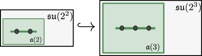
Figure 2: Growing a Lie algebra by adding a site to the chain.

The above example illustrates that the algebraic structure of a DLA can change as we increase the system size. Additionally, when we extend the number of sites to $n>2$, we need to take into account what happens at the edge of the chain. For $1$-dimensional systems, this leads to two cases: open boundary conditions (operators on a line) and periodic boundary conditions (operators on a circle). We will denote the resulting DLAs of these two cases with $\mathfrak{g}$ and $\mathfrak{g}^{\circ}$, respectively. Additionally, we distinguish between Hamiltonians generated by Pauli strings that consist of two Pauli operators both different from $I$ (e.g. $\{XY,XZ\}$) and Hamiltonians generated by Pauli strings that include the identity (e.g. $\{IX,ZI,XX\}$). We denote the Lie algebras generated by the former as $\mathfrak{a}$ and the Lie algebras generated by the latter as $\mathfrak{b}$.

III Method

We can now state the central question of our work. Given a Hamiltonian of the form (2), we seek a classification of all DLAs generated by the terms of the Hamiltonian, for $n\geq 3$ with both open and periodic boundary conditions.

III.1 The power sets

First, for the generators of $\mathfrak{a}$-type Lie algebras, we note that there are 9 Pauli strings that consist of two Pauli operators. Hence, the power set of the possible generators $\mathcal{A}$ contains $2^{9}-1=511$ elements. Similarly, for the $\mathfrak{b}$-type Lie algebras, there are 15 Pauli strings, which results in a power set of $2^{15}-1=32767$ possible sets of generators. Clearly, the sets of generators of the $\mathfrak{a}$-type are included in the $\mathfrak{b}$-type power set. We thus only report the $\mathfrak{b}$-type Lie algebras that are not also $\mathfrak{a}$-types. There is a third class of Lie algebras, the $\mathfrak{c}$-type Lie algebras, which are an edge case where the generators contain only Pauli strings of the form $a\otimes I$, but not the corresponding term $I\otimes a$. The structure of these Lie algebras is captured by the $\mathfrak{b}$-type Lie algebras, except for a small boundary effect at the last site in the chain. We therefore exclude the $\mathfrak{c}$-type Lie algebras from our classification.

We proceed by going through all sets of generators $\mathcal{A}$ (of either $\mathfrak{a}$ or $\mathfrak{b}$-type) and use Algorithm 1 to perform the nested commutators in (1). We then store only the unique subalgebras generated by this procedure, and we obtain only $127$ and $19$ generating sets for $\mathfrak{a}$-type and $\mathfrak{b}$-type, respectively. Since the largest power set we consider has only $32767$ elements, this procedure can be performed numerically with ease. We provide the code to reproduce this at [43].

Example III.1.

Consider the generating sets:

$$\mathcal{A}_{1} =\{XY,XZ\},$$

$$\mathcal{A}_{2} =\{IX,XY\}.$$

Note that $\mathcal{A}_{1}$ is of $\mathfrak{a}$-type and $\mathcal{A}_{2}$ is of $\mathfrak{c}$-type. After running Algorithm 1, we find:

$$\langle\mathcal{A}_{1}\rangle_{\mathrm{Lie}} =\mathrm{span}\{XY,XZ,IX\},$$

$$\langle\mathcal{A}_{2}\rangle_{\mathrm{Lie}} =\mathrm{span}\{IX,XY,XY\}.$$

We see that $\mathcal{A}_{1}$ and $\mathcal{A}_{2}$ generate the same Lie algebra; hence, this Lie algebra is counted among the $\mathfrak{a}$-type Lie algebras.

Example III.2.

Consider the generating sets of $\mathfrak{a}$-type:

$$\mathcal{A}_{1} =\{XX,YY\},$$

$$\mathcal{A}_{2} =\{XX,YX\}.$$

After running Algorithm 1, we find:

$$\langle\mathcal{A}_{1}\rangle_{\mathrm{Lie}} =\mathrm{span}\{XX,YY\},$$

$$\langle\mathcal{A}_{2}\rangle_{\mathrm{Lie}} =\mathrm{span}\{XX,YX,ZX\}.$$

Hence, $\mathcal{A}_{1}$ and $\mathcal{A}_{2}$ generate distinct Lie algebras, both of $\mathfrak{a}$-type.

Example III.3.

The set of $\mathfrak{b}$-type

$$\mathcal{A}=\{XY,XI,IX\}$$

generates the Lie algebra

$$\langle\mathcal{A}\rangle_{\mathrm{Lie}}=\mathrm{span}\{XY,XZ,XI,IX\}.$$

If we try to generate it from the $\mathfrak{a}$-type subset $\{XY,XZ\}$, we find the strictly smaller subalgebra

$$\langle XY,XZ\rangle_{\mathrm{Lie}}=\mathrm{span}\{XY,XZ,IX\}.$$

III.2 Symmetries of the power sets

There are certain symmetries that can be exploited to reduce the number of subalgebras of $\mathfrak{su}(4)$ in the above power sets. To start, we note that the Pauli matrices satisfy the following algebraic relations:

$$[\sigma^{\alpha},\sigma^{\beta}]=2i\sum_{\gamma=1}^{3}\epsilon_{\alpha\beta\gamma}\sigma^{\gamma},$$

where $\epsilon_{\alpha\beta\gamma}$ is the Levi-Civita tensor and $\alpha,\beta,\gamma\in\{1,2,3\}$, respectively (see SM I for more details). We will ignore the factor $2i$, since we only care about the linear span of nested commutators. Note that the above relation is independent of how we assign $X,Y,Z$ to $\sigma^{\alpha}$. In other words, we can relabel the Paulis and retain the algebraic structure of the subalgebras, which together with ignoring the prefactors formally corresponds to an $S_{3}$ permutation symmetry.

In addition to relabelling, we consider the exchange of location of the two Pauli terms, since the order of such terms is an arbitrary choice that does not impact the structure of the resulting Lie algebras. This location exchange corresponds to a $\mathbb{Z}_{2}$ symmetry. Hence, the symmetry group of the Pauli algebra for $n=2$ is $S_{3}\times\mathbb{Z}_{2}$. Subalgebras of $\mathfrak{su}(4)$ that are in the same orbit of this symmetry group are considered equivalent, which allows us to reduce the number of subalgebras significantly.

Example III.4.

We have that $\{XX,YZ\}\equiv\{YY,ZX\}$ under relabeling $X\to Y\to Z\to X$. On the other hand, $\{XX,YZ\}$ and $\{XX,YY\}$ are not equivalent.

In order to determine the orbits of the symmetry group $S_{3}\times\mathbb{Z}_{2}$ on the set of subalgebras of $\mathfrak{su}(4)$, we introduce their invariants $s,p,e,d$, defined as follows. These enumerate the number of single Paulis (such as $XI$) in the basis of the Lie algebra, the number of single Pauli pairs (such as $XI,IX$), the number of double equal Paulis (such as $XX$) and the number of double different Paulis (such as $XY$), respectively. Since all these quantities are invariant under the action of the symmetry group, two subalgebras are not equivalent if they have different invariant.

Example III.5.

Consider the following bases of subalgebras and their invariants:

$$\mathcal{A}_{1} =\{ZZ,YX,XY\}\to(0,0,1,2),$$

$$\mathcal{A}_{2} =\{XX,YZ,ZY\}\to(0,0,1,2),$$

$$\mathcal{A}_{3} =\{YY,ZX,XZ\}\to(0,0,1,2).$$

We see that $\mathcal{A}_{1}\equiv\mathcal{A}_{2}$ under $Z\rightleftharpoons X$. Similarly, $\mathcal{A}_{2}\equiv\mathcal{A}_{3}$ under $X\rightleftharpoons Y$ and $\mathcal{A}_{3}\equiv\mathcal{A}_{1}$ under $Y\rightleftharpoons Z$.

Example III.6.

Consider the following bases of subalgebras and their invariants:

$$\mathcal{A}_{1} =\{XX,XZ,IY\}\to(1,0,1,1),$$

$$\mathcal{A}_{2} =\{XY,XZ,IX\}\to(1,0,0,2).$$

We see that $\mathcal{A}_{1}\not\equiv\mathcal{A}_{2}$, since they have different invariants.

Example III.7.

Even though the two bases

$$\mathcal{A}_{1} =\{XY,YX\}\to(0,0,0,2),$$

$$\mathcal{A}_{2} =\{XY,YZ\}\to(0,0,0,2)$$

have the same invariants, they are not equivalent under the symmetry group $S_{3}\times\mathbb{Z}_{2}$.

Carrying out this procedure exhaustively for the $127$ and $19$ subalgebras of $\mathfrak{a}$-type and $\mathfrak{b}$-type gives us $23$ and $5$ inequivalent Lie algebras, respectively. We denote these subalgebras by $\mathfrak{a}_{k}$ $(0\leq k\leq 22)$ and $\mathfrak{b}_{l}$ $(0\leq l\leq 4)$. For the full list of invariants, see Table S.I in the Supplemental Materials. In particular, it turns out that the only case in which the invariants $(s,p,e,d)$ cannot distinguish inequivalent subalgebras is that presented in Example III.7.

By Proposition I.1, we can identify these subalgebras by inspection with direct sums of simple Lie algebras plus a center.

Example III.8.

The set

$$\mathcal{A}=\{XX,YY,ZZ,ZY\}$$

generates the Lie algebra

$$\mathfrak{a}_{20}:=\langle\mathcal{A}\rangle_{\mathrm{Lie}}=\mathrm{span}\{XX,YY,ZZ,YZ,ZY,XI,IX\}$$

$$=\mathrm{span}\{YY+ZZ,YZ+ZY,XI+IX\}$$

$$\oplus\mathrm{span}\{YY-ZZ,YZ-ZY,XI-IX\}\oplus\mathrm{span}\{XX\}$$

$$\cong\mathfrak{su}(2)\oplus\mathfrak{su}(2)\oplus\mathfrak{u}(1).$$

At this point, we have reduced the number of possible Hamiltonians in our class significantly by taking into account the symmetries of the Pauli group. As a final step, we now generate all $\mathfrak{a}_{k}(n)$, $\mathfrak{b}_{k}(n)$, $\mathfrak{a}^{\circ}_{k}(n)$ and $\mathfrak{b}_{k}^{\circ}(n)$ up to $n=8$. With knowledge of the structure of the Lie algebras for $3\leq n\leq 8$, we can construct formal proofs to determine them for all $n\geq 3$, which is discussed in the next section.

IV Results

IV.1 Main theorem

We state the main theorem of our work below, and tabulate the generators of the Lie algebras of our classification in Table 1.

Theorem IV.1 (Classification of DLAs).

The complete list of dynamical Lie algebras of translation-invariant $2$-local Hamiltonians in one dimension of length $n\geq 3$ is:

$$\mathfrak{a}_{0}(n) \cong\mathfrak{u}(1)^{\oplus(n-1)},$$

$$\mathfrak{a}_{1}(n) \cong\mathfrak{so}(n),$$

$$\mathfrak{a}_{2}(n) \cong\mathfrak{a}_{4}(n)\cong\mathfrak{so}(n)\oplus\mathfrak{so}(n),$$

$$\mathfrak{a}_{3}(n) \cong\begin{cases}\mathfrak{so}(2^{n-2})^{\oplus 4},&n\equiv 0\;\mathrm{mod}\;8,\\ \mathfrak{so}(2^{n-1}),&n\equiv\pm 1\;\mathrm{mod}\;8,\\ \mathfrak{su}(2^{n-2})^{\oplus 2},&n\equiv\pm 2\;\mathrm{mod}\;8,\\ \mathfrak{sp}(2^{n-2}),&n\equiv\pm 3\;\mathrm{mod}\;8,\\ \mathfrak{sp}(2^{n-3})^{\oplus 4},&n\equiv 4\;\mathrm{mod}\;8,\end{cases}$$

$$\mathfrak{a}_{5}(n) \cong\begin{cases}\mathfrak{so}(2^{n-2})^{\oplus 4},&n\equiv 0\;\mathrm{mod}\;6,\\ \mathfrak{so}(2^{n-1}),&n\equiv\pm 1\;\mathrm{mod}\;6,\\ \mathfrak{su}(2^{n-2})^{\oplus 2},&n\equiv\pm 2\;\mathrm{mod}\;6,\\ \mathfrak{sp}(2^{n-2}),&n\equiv 3\;\mathrm{mod}\;6,\end{cases}$$

$$\mathfrak{a}_{6}(n) \cong\mathfrak{a}_{7}(n)\cong\mathfrak{a}_{10}(n)$$

$$\cong\begin{cases}\mathfrak{su}(2^{n-1}),&n\;\;\mathrm{odd},\\ \mathfrak{su}(2^{n-2})^{\oplus 4},&n\geq 4\;\;\mathrm{even},\end{cases}$$

$$\mathfrak{a}_{8}(n) \cong\mathfrak{so}(2n-1),$$

$$\mathfrak{a}_{9}(n) \cong\mathfrak{sp}(2^{n-2}),$$

$$\mathfrak{a}_{11}(n) =\mathfrak{a}_{16}(n)=\mathfrak{so}(2^{n}),\quad n\geq 4,$$

$$\mathfrak{a}_{k}(n) =\mathfrak{su}(2^{n}),\;\;k=12,17,18,19,21,22,\;n\geq 4,$$

$$\mathfrak{a}_{13}(n) =\mathfrak{a}_{20}(n)\cong\mathfrak{a}_{15}(n)\cong\mathfrak{su}(2^{n-1})^{\oplus 2},$$

$$\mathfrak{a}_{14}(n) \cong\mathfrak{so}(2n),$$

$$\mathfrak{b}_{0}(n) \cong\mathfrak{u}(1)^{\oplus n},$$

$$\mathfrak{b}_{1}(n) \cong\mathfrak{u}(1)^{\oplus(2n-1)},$$

$$\mathfrak{b}_{2}(n) \cong\mathfrak{sp}(2^{n-2})\oplus\mathfrak{u}(1),$$

$$\mathfrak{b}_{3}(n) \cong\mathfrak{su}(2)^{\oplus n},$$

$$\mathfrak{b}_{4}(n) \cong\mathfrak{su}(2^{n-1})\oplus\mathfrak{su}(2^{n-1})\oplus\mathfrak{u}(1).$$

Label	Generating set	Model
$\mathfrak{a}_{0}$	$XX$	Ising model
$\mathfrak{a}_{1}$	$XY$	Kitaev chain
$\mathfrak{a}_{2}$	$XY,YX$	Massless free fermion +
		magnetic field
$\mathfrak{a}_{3}$	$XX,YZ$	Kitaev chain + Coulomb
$\mathfrak{a}_{4}$	$XX,YY$	XY-model
$\mathfrak{a}_{5}$	$XY,YZ$
$\mathfrak{a}_{6}$	$XX,YZ,ZY$	Massless free fermion +
		magnetic field + Coulomb
$\mathfrak{a}_{7}$	$XX,YY,ZZ$	Heisenberg chain
$\mathfrak{a}_{8}$	$XX,XZ$	Ising model + transverse field
$\mathfrak{a}_{9}$	$XY,XZ$	Kitaev chain + longitudinal field
$\mathfrak{a}_{10}$	$XY,YZ,ZX$	Heisenberg
$\mathfrak{a}_{11}$	$XY,YX,YZ$	XY-model + longitudinal field
$\mathfrak{a}_{12}$	$XX,XY,YZ$
$\mathfrak{a}_{13}$	$XX,YY,YZ$	XY-model + longitudinal field
$\mathfrak{a}_{14}$	$XX,YY,XY$	XY-model + transverse field
$\mathfrak{a}_{15}$	$XX,XY,XZ$	Ising model + arbitrary field
$\mathfrak{a}_{16}$	$XY,YX,YZ,ZY$	Kitaev chain + longitudinal field
$\mathfrak{a}_{17}$	$XX,XY,ZX$	Ising model + arbitrary field
$\mathfrak{a}_{18}$	$XX,XZ,YY,ZY$	XY-model + arbitrary field
$\mathfrak{a}_{19}$	$XX,XY,ZX,YZ$
$\mathfrak{a}_{20}$	$XX,YY,ZZ,ZY$	Heisenberg chain + magnetic field
$\mathfrak{a}_{21}$	$XX,YY,XY,ZX$	XY-model + arbitrary field
$\mathfrak{a}_{22}$	$XX,XY,XZ,YX$	Ising model + arbitrary field
$\mathfrak{b}_{0}$	$XI,IX$	Uncoupled spins
$\mathfrak{b}_{1}$	$XX,XI,IX$	Ising model
$\mathfrak{b}_{2}$	$XY,XI,IX$	Kitaev chain + longitudinal field
$\mathfrak{b}_{3}$	$XI,YI,IX,IY$	Uncoupled spins
$\mathfrak{b}_{4}$	$XX,XY,XZ,XI,$ $IX,IY,IZ$	Ising model + arbitrary field

Table 1: List of generators of the DLAs in Theorem IV.1 and corresponding conventional spin models.

The following corollary immediately follows from Theorem IV.1 and knowledge of the dimensions of $\mathfrak{su}$, $\mathfrak{so}$ and $\mathfrak{sp}$ (see (A9)).

Corollary IV.1 (Dimension scaling of DLAs).

The dimension of all non-trivial DLAs of translation-invariant $2$-local Hamiltonians of length $n$ will scale as either $O(4^{n})$, $O(n^{2})$ or $O(n)$.

We thus see that the DLAs can be separated in three classes based on the scaling of their dimensions.

IV.2 Sketch of the proof

The complete proof of Theorem IV.1 is presented in the Supplemental Materials. Here is a brief sketch of the proof; we refer to SM I for a more detailed outline. We divide the set of Lie algebras $\mathfrak{a}_{k}(n)$, $\mathfrak{b}_{l}(n)$ into three classes: linear, quadratic, and exponential, according to the anticipated growth of their dimension. The linear class consists of $\mathfrak{a}_{0}(n)$ and $\mathfrak{b}_{l}(n)$ with $l=0,1,3$, and their treatment is obvious. The quadratic class contains $\mathfrak{a}_{k}(n)$ with $k=1,2,4,8,14$. These Lie algebras are determined by using the frustration graphs of their generators in SM III. For the exponential class, we first observe that $\mathfrak{b}_{2}(n)=\mathfrak{a}_{9}(n)\oplus\mathrm{span}\{X_{1}\}$ and $\mathfrak{b}_{4}(n)=\mathfrak{a}_{15}(n)\oplus\mathrm{span}\{X_{1}\}$. Next, we identify the cases when $\mathfrak{a}_{k}(n)=\mathfrak{su}(2^{n})$; see SM IV for details. We also find isomorphisms that are obtained by relabeling of the Pauli matrices among some of the algebras (SM II).

The strategy in the remaining exponential cases is as follows.

1. For each of our Lie subalgebras $\mathfrak{s}=\mathfrak{a}_{k}(n)\subseteq\mathfrak{su}(2^{n})$, we find its stabilizer $\mathrm{St}(\mathfrak{s})$, which is defined as the set of all Pauli strings $\in\mathcal{P}_{n}$ that commute with every element of $\mathfrak{s}$. This can be done explicitly, because the stabilizer is determined only from the generators of $\mathfrak{s}$ (see Proposition C.3).

2. By definition, $\mathfrak{s}$ commutes with all elements of its stabilizer $\mathrm{St}(\mathfrak{s})$; hence, it is contained in the centralizer of $\mathrm{St}(\mathfrak{s})$ in $\mathfrak{su}(2^{n})$, which we denote $\mathfrak{su}(2^{n})^{\mathrm{St}(\mathfrak{s})}$. We can reduce the Lie subalgebra $\mathfrak{su}(2^{n})^{\mathrm{St}(\mathfrak{s})}$ further by factoring all elements of the center of $\mathrm{St}(\mathfrak{s})$, which will become central in it, because we have shown that $\mathfrak{s}$ has a trivial center (Lemma C.11). This results in a Lie algebra denoted $\mathfrak{g}_{k}(n)$ when $\mathfrak{s}=\mathfrak{a}_{k}(n)$.

3. By the above construction, we have $\mathfrak{a}_{k}(n)\subseteq\mathfrak{g}_{k}(n)$. In the case of associative algebras, we would get equality due to (a finite-dimensional version of) von Neumann’s Double Commutant Theorem (see e.g. [44], Theorem 6.2.5). However, in the Lie case, we might have a strict inclusion. We improve the upper bounds for $\mathfrak{a}_{k}(n)$ by finding involutions $\theta_{k}$ of $\mathfrak{g}_{k}(n)$ such that all elements of $\mathfrak{a}_{k}(n)$ are fixed under $\theta_{k}$. The last condition can be checked only on the generators of $\mathfrak{a}_{k}(n)$ (see SM V).

4. We prove by induction on $n$ that the upper bound is exact, that is $\mathfrak{a}_{k}(n)=\mathfrak{g}_{k}(n)^{\theta_{k}}$ (see SM VI). First we note that both $\mathfrak{a}_{k}(n)$ and $\mathfrak{g}_{k}(n)^{\theta_{k}}$ are linearly spanned by the Pauli strings contained in them. We start with an arbitrary Pauli string $a\in i\mathcal{P}_{n}\cap\mathfrak{g}_{k}(n)^{\theta_{k}}$ and want to show that it is in $\mathfrak{a}_{k}(n)$. The main idea is to use suitable commutators of $a$ with elements of $\mathfrak{a}_{k}(n)$ to produce a Pauli string $b\in i\mathcal{P}_{n}\cap\mathfrak{g}_{k}(n)^{\theta_{k}}$ with $I$ in one of its positions. Erasing the $I$ in $b$ gives an element of $\mathfrak{g}_{k}(n-1)^{\theta_{k}}$, which by induction is in $\mathfrak{a}_{k}(n-1)$.

5. Finally, we identify the Lie algebras $\mathfrak{g}_{k}(n)^{\theta_{k}}$ with those from Theorem IV.1 (see SM VII). This is accomplished by applying in each case a suitable unitary transformation that brings the stabilizer $\mathrm{St}(\mathfrak{s})$ to a more convenient form (cf. SM III).

IV.3 Example: $\mathfrak{a}_{9}(n)$

Consider the example of $\mathfrak{a}_{9}=\langle XY,XZ\rangle_{\mathrm{Lie}}$, which produces the subalgebra $\mathfrak{a}_{9}(n)\subseteq\mathfrak{su}(2^{n})$ generated by:

$$X_{1}Y_{2},X_{1}Z_{2},X_{2}Y_{3},X_{2}Z_{3},\dots,X_{n-1}Y_{n},X_{n-1}Z_{n}.$$ (4)

Let us sketch the above steps in the strategy of the proof of Theorem IV.1 in the case $\mathfrak{s}=\mathfrak{a}_{9}(n)$.

1. The stabilizer $\mathrm{St}(\mathfrak{s})$ is the set of all Pauli strings $P\in\mathcal{P}_{n}$ such that $[a,P]=0$ for every $a\in\mathfrak{s}$. It is enough to check this for all $a$ in the list of generators (4), which means that the substring of $P$ in positions $j,j+1$ commutes with $XY$ and $XZ$ for all $1\leq j\leq n-1$. By inspection, we find $\mathrm{St}(XY,XZ)=\{II,XI,YX,ZX\}$, so these are the only possible such substrings of $P$. This gives $\mathrm{St}(\mathfrak{s})=\{I^{\otimes n},X_{1},Y_{1}X_{2},Z_{1}X_{2}\}$.

2. The centralizer $\mathfrak{su}(2^{n})^{\mathrm{St}(\mathfrak{s})}$ is the set of all $a\in\mathfrak{su}(2^{n})$ such that $[a,P]=0$ for every $P\in\mathrm{St}(\mathfrak{s})$; hence it contains $\mathfrak{s}$. As the center of $\mathrm{St}(\mathfrak{s})$ is trivial, we have $\mathfrak{g}_{9}(n)=\mathfrak{su}(2^{n})^{\mathrm{St}(\mathfrak{s})}$. To illustrate this last step, we mention that $\mathrm{St}(\mathfrak{a}_{15}(n))=\{I^{\otimes n},X_{1}\}$. In this case, $X_{1}\in\mathfrak{su}(2^{n})^{X_{1}}$ is central and we have to quotient by it to obtain $\mathfrak{g}_{15}(n)=\mathfrak{su}(2^{n})^{X_{1}}/\mathrm{span}\{X_{1}\}$.

3. We saw above that $\mathfrak{s}\subseteq\mathfrak{g}_{9}(n)$. Now we find an involution $\theta_{9}$ of $\mathfrak{g}_{9}(n)$ such that $\mathfrak{s}\subseteq\mathfrak{g}_{9}(n)^{\theta_{9}}$, the set of fixed points under $\theta_{9}$. Since $\theta_{9}$ respects the Lie brackets, it is enough to check $\theta_{9}(a)=a$ only for the generators (4). Explicitly, we let $\theta_{9}(a)=-Q_{9}a^{T}Q_{9}$ where $Q_{9}=IYZZ\cdots Z$.

4. We prove by induction on $n$ that $\mathfrak{a}_{9}(n)=\mathfrak{g}_{9}(n)^{\theta_{9}}$. To show that any $a\in i\mathcal{P}_{n}\cap\mathfrak{g}_{9}(n)^{\theta_{9}}$ with $n\geq 4$ is in $\mathfrak{a}_{9}(n)$, we first take suitable commutators of $a$ with the generators (4) to produce $b\in i\mathcal{P}_{n}\cap\mathfrak{g}_{k}(n)^{\theta_{k}}$ that has $I$ in some position $j\geq 3$. Erasing the $I$ gives an element $c\in\mathfrak{g}_{9}(n-1)^{\theta_{9}}$, which by induction is in $\mathfrak{a}_{9}(n-1)$. Inserting $I$ back in $j$-th place in $c$ gives that $b\in\mathfrak{a}_{9}(n)$.

5. As $\mathrm{St}(\mathfrak{s})\cong\{I^{\otimes n},X_{1},Y_{1},Z_{1}\}$, we can simplify $\mathfrak{g}_{9}(n)^{\theta_{9}}$ by applying a unitary transformation $a\mapsto UaU^{\dagger}$ that takes $\mathrm{St}(\mathfrak{s})$ to $\{I^{\otimes n},X_{1},Y_{1},Z_{1}\}$. Explicitly, we take $U=e^{i\frac{\pi}{4}X_{1}X_{2}}$. Then $\mathfrak{g}_{9}(n)\cong\mathfrak{su}(2^{n})^{\{X_{1},Y_{1},Z_{1}\}}=I\otimes\mathfrak{su}(2^{n-1})\cong\mathfrak{su}(2^{n-1})$. The involution $\theta_{9}(a)=-Q_{9}a^{T}Q_{9}$ gets transformed to $-\tilde{Q}_{9}a^{T}\tilde{Q}_{9}$, where $\tilde{Q}_{9}=UQ_{9}U^{T}$ in this case happens to be $=Q_{9}$. Restricted to $\mathfrak{su}(2^{n-1})$, this gives the involution $-Qa^{T}Q$ with $Q=YZZ\cdots Z$, whose fixed points are $\cong\mathfrak{sp}(2^{n-2})$ because $Q^{T}=-Q$.

We conclude that $\mathfrak{a}_{9}(n)\cong\mathfrak{sp}(2^{n-2})$.

IV.4 Periodic boundary conditions

For the periodic case, we have the same sets of generators as in Theorem IV.1, but we need to adapt our proof strategy, because, unlike the open case, the periodic Lie algebras $\mathfrak{a}_{k}^{\circ}(n)$ are not generated inductively from $\mathfrak{a}_{k}^{\circ}(n-1)$. Instead, we use that $\mathfrak{a}_{k}^{\circ}(n)$ is generated from $\mathfrak{a}_{k}(n)$ and its cyclic shifts, and we utilize the explicit description $\mathfrak{a}_{k}(n)=\mathfrak{g}_{k}(n)^{\theta_{k}}$ (see Part 4. in Sect. IV.2, and for more details SM VI).

Theorem IV.2 (Classification of Periodic DLAs).

The complete list of dynamical Lie algebras of translation-invariant periodic $2$-local Hamiltonians in one dimension of length $n\geq 3$ is:

$$\mathfrak{a}_{0}^{\circ}(n) \cong\mathfrak{u}(1)^{\oplus n},$$

$$\mathfrak{a}_{1}^{\circ}(n) \cong\mathfrak{so}(n)^{\oplus 2},$$

$$\mathfrak{a}_{2}^{\circ}(n) \cong\mathfrak{so}(n)^{\oplus 4},$$

$$\mathfrak{a}_{3}^{\circ}(n) =\begin{cases}\mathfrak{a}_{13}(n),&n\;\;\mathrm{odd},\\ \mathfrak{a}_{3}(n),&n\equiv 0\mod 4,\\ \mathfrak{a}_{6}(n),&n\equiv 2\mod 4,\end{cases}$$

$$\cong\begin{cases}\mathfrak{su}(2^{n-1})^{\oplus 2},&n\;\;\mathrm{odd},\\ \mathfrak{so}(2^{n-2})^{\oplus 4},&n\equiv 0\mod 8,\\ \mathfrak{sp}(2^{n-3})^{\oplus 4},&n\equiv 4\mod 8,\\ \mathfrak{su}(2^{n-2})^{\oplus 4},&n\equiv 2\mod 4,\end{cases}$$

$$\mathfrak{a}_{4}^{\circ}(n) \cong\begin{cases}\mathfrak{so}(2n),\quad\;\;n\;\;\mathrm{odd},\\ \mathfrak{so}(n)^{\oplus 4},\quad n\;\mathrm{even},\end{cases}$$

$$\mathfrak{a}_{5}^{\circ}(n) =\begin{cases}\mathfrak{a}_{16}(n),&n\equiv\pm 1\mod 3,\\ \mathfrak{a}_{5}(n),&n\equiv 0\mod 3,\end{cases}$$

$$\cong\begin{cases}\mathfrak{so}(2^{n}),&n\equiv\pm 1\mod 3,\\ \mathfrak{so}(2^{n-2})^{\oplus 4},&n\equiv 0\mod 6,\\ \mathfrak{sp}(2^{n-2}),&n\equiv 3\mod 6,\end{cases}$$

$$\mathfrak{a}_{6}^{\circ}(n) =\begin{cases}\mathfrak{a}_{13}(n)\cong\mathfrak{su}(2^{n-1})^{\oplus 2},&n\;\;\mathrm{odd},\\ \mathfrak{a}_{6}(n)\cong\mathfrak{su}(2^{n-2})^{\oplus 4},&n\;\;\mathrm{even},\end{cases}$$

$$\mathfrak{a}_{k}^{\circ}(n) =\mathfrak{a}_{k}(n),\quad k=7,13,16,20,$$

$$\mathfrak{a}_{8}^{\circ}(n) \cong\mathfrak{so}(2n)^{\oplus 2},$$

$$\mathfrak{a}_{9}^{\circ}(n) \cong\mathfrak{so}(2^{n}),\quad n\geq 4,$$

$$\mathfrak{a}_{10}^{\circ}(n) =\begin{cases}\mathfrak{su}(2^{n}),&n\equiv\pm 1\mod 3,\\ \mathfrak{a}_{10}(n),&n\equiv 0\mod 3,\end{cases}$$

$$\cong\begin{cases}\mathfrak{su}(2^{n}),&n\equiv\pm 1\mod 3,\\ \mathfrak{su}(2^{n-2})^{\oplus 4},&n\equiv 0\mod 6,\\ \mathfrak{su}(2^{n-1}),&n\equiv 3\mod 6,\end{cases}$$

$$\mathfrak{a}_{11}^{\circ}(n) =\mathfrak{so}(2^{n}),\quad n\geq 4,$$

$$\mathfrak{a}_{k}^{\circ}(n) =\mathfrak{su}(2^{n}),\;\;k=12,15,17,18,19,21,22,$$

$$\mathfrak{a}_{14}^{\circ}(n) \cong\mathfrak{so}(2n)^{\oplus 2},$$

$$\mathfrak{b}_{0}^{\circ}(n) =\mathfrak{b}_{0}(n)\cong\mathfrak{u}(1)^{\oplus n},$$

$$\mathfrak{b}_{1}^{\circ}(n) \cong\mathfrak{u}(1)^{\oplus 2n},$$

$$\mathfrak{b}_{2}^{\circ}(n) \cong\mathfrak{so}(2^{n}),\quad n\geq 4,$$

$$\mathfrak{b}_{3}^{\circ}(n) =\mathfrak{b}_{3}(n)\cong\mathfrak{su}(2)^{\oplus n},$$

$$\mathfrak{b}_{4}^{\circ}(n) =\mathfrak{su}(2^{n}).$$

The proof of this theorem is given in SM VIII.

IV.5 Permutation-invariant subalgebras

The strategies employed for periodic boundary conditions can also be used to classify the DLAs in the case when the Hamiltonian is defined on a permutation-invariant graph. Now each spin is connected to each other spin via $2$-local interactions given by Pauli strings. We denote the resulting DLAs by $\mathfrak{g}^{\pi}$. As this is not the main focus of our work, we simply state the result here and provide the details in the Supplemental Materials.

Theorem IV.3 (Classification of Permutation Invariant DLAs).

The complete list of dynamical Lie algebras of permutation-invariant $2$-site Hamiltonians in one dimension of length $n\geq 3$ is:

$$\mathfrak{a}_{k}^{\pi}(n) =\mathfrak{a}_{k}(n),\qquad k=7,16,20,22,$$

$$\mathfrak{a}_{0}^{\pi}(n) \cong\mathfrak{u}(1)^{\oplus n(n-1)/2},$$

$$\mathfrak{a}_{2}^{\pi}(n) =\mathfrak{so}(2^{n})^{Z\cdots Z}\cong\mathfrak{so}(2^{n-1})^{\oplus 2},$$

$$\mathfrak{a}_{4}^{\pi}(n) =\mathfrak{a}_{7}(n)\cong\begin{cases}\mathfrak{su}(2^{n-1}),&n\;\;\mathrm{odd},\\ \mathfrak{su}(2^{n-2})^{\oplus 4},&n\geq 4\;\;\mathrm{even},\end{cases}$$

$$\mathfrak{a}_{6}^{\pi}(n) =\mathfrak{a}_{20}(n)\cong\mathfrak{a}_{14}^{\pi}(n)\cong\mathfrak{su}(2^{n-1})^{\oplus 2},$$

$$\mathfrak{b}_{0}^{\pi}(n) =\mathfrak{b}_{0}(n)\cong\mathfrak{u}(1)^{\oplus n},$$

$$\mathfrak{b}_{1}^{\pi}(n) \cong\mathfrak{u}(1)^{\oplus n(n+1)/2},$$

$$\mathfrak{b}_{3}^{\pi}(n) =\mathfrak{b}_{3}(n)\cong\mathfrak{su}(2)^{\oplus n}.$$

The proof of this theorem is given in SM IV.5.

V Discussion

In the previous section, we classified all DLAs of $2$-local spin chain Hamiltonians in one dimension. In this section, we discuss the importance of this classification for various fields in physics.

V.1 Relevance for quantum control

In quantum control, one is interested in performing a specific unitary evolution. This can be achieved by controlling some physical system described by a Hamiltonian $H$, parameterized by controls $\lambda(t)\in\mathbb{R}$ at each time step,

$$H=\sum_{k=1}^{|\mathcal{A}|}\lambda_{k}(t)a_{k},$$

where $\mathcal{A}$ is now any set of operators $a_{k}$ that can be physically implemented. The set of unitaries that can be realized after a certain time $T\geq 0$ is then determined by the Schrödinger equation in the Heisenberg picture (after setting $\hbar=1$):

$$\frac{dU}{dt}=-iH(\lambda(t))\,U(t),\qquad U(0)=I.$$

If the set of unitaries that can be reached after time $T$ is the full unitary group, the system is said to be (operator) controllable [40]. This is a desirable property when one is interested in building a quantum computer with a universal gate set.

To test whether a system is controllable, one determines the DLA $\langle\mathcal{A}\rangle_{\mathrm{Lie}}$ and checks if it equals $\mathfrak{su}(2^{n})$. The conditions for complete controllability are known [22], and it is in principle easy to create a controllable system since any real simple Lie algebra can be generated from $2$ elements [45]. If the DLA is a proper subalgebra of $\mathfrak{su}(2^{n})$, we say that the system is uncontrollable. Note that this includes simple Lie algebras like $\mathfrak{so}$ and $\mathfrak{sp}$ [23]. Uncontrollable systems can arise when there are conserved quantities or symmetries in the physical system one is trying to control. Note that, due to Proposition I.1, the DLA must split into a direct sum of simple Lie algebras and a center. If all simple summands in this decomposition are of the form $\mathfrak{su}$, then we say that the system is subspace controllable [40].

We can contextualize our classification in terms of these definitions. For example, we know that $\mathfrak{a}_{12}(n)$ will produce a controllable quantum system for $n\geq 4$ since this DLA is equal to $\mathfrak{su}(2^{n})$. Similarly, since $\mathfrak{a}_{1}(n)\cong\mathfrak{so}(n)$, we know that it is uncontrollable. Finally, there are many examples of uncontrollable systems that consist of direct sums of $\mathfrak{su}$ blocks; hence are subspace controllable. For instance, $\mathfrak{a}_{3}^{\circ}(n)$ for odd $n$ produces a DLA of the form $\mathfrak{su}(2^{n-1})^{\oplus 2}$.

In addition to the notion of controllability of spin systems, we can ask what other types of systems we can simulate with our spin chains, e.g., fermionic or bosonic systems. This question was originally explored for Hamiltonians on cubic lattices with translation symmetry [46, 47]. In particular, the dynamics of quadratic fermionic Hamiltonians is described by DLAs of the $\mathfrak{so}(2n)$ or $\mathfrak{so}(2n+1)$ type, which show up in our classification as $\mathfrak{a}_{14}(n)$ and $\mathfrak{a}_{8}(n)$. Similarly, the dynamics of a bosonic quadratic Hamiltonian with $n$ modes is related to a symplectic DLA [25], which we can identify with $\mathfrak{a}_{5}(n)$ for $n\equiv 3$ mod $6$. Finally, one can consider composite systems and explore which subgroups of $\mathrm{SU}(N)$ can generated in this manner [48].

V.2 Relevance for variational quantum computing

A quantum circuit can be described as a product of unitaries $U=\prod_{k}U_{k}$. Typically, the quantum circuit $U$ acts on a multi-qubit state, whereas the gates $U_{k}$ only act on single or two qubit subsystems, i.e., we can write $U_{k}=e^{a_{k}}$ where $a_{k}$ is a $1$- or $2$-local operator. For a set of generators $\mathcal{A}=\{a_{k}\}$ with a corresponding DLA $\mathfrak{a}=\langle\mathcal{A}\rangle_{\mathrm{Lie}}$, we have that

$$e^{\mathfrak{a}}=\bigl{\{}e^{a_{k_{1}}t_{1}}e^{a_{k_{2}}t_{2}}\cdots e^{a_{k_{r}}t_{r}}\,\big{|}\,t_{i}\in\mathbb{R},\;a_{k_{i}}\in\mathcal{A}\bigr{\}}.$$ (5)

In other words, any element in the Lie group $e^{\mathfrak{a}}$ generated by the DLA can be reached by a finite product of unitaries in that group (see [40], Corollary 3.2.6). In quantum computing, if $e^{\mathfrak{a}}=\mathrm{SU}(2^{n})$, then the gate set $\{e^{a_{k}}\}$ is called universal [49]. It is known that almost any combination of unitaries is universal [50, 51]. However, we can make specific choices for the generators $\{a_{k}\}$ that correspond to a non-universal gate set, which instead will generate a proper subgroup of $\mathrm{SU}(2^{n})$. This is especially relevant for a class of quantum algorithms called variational quantum algorithms [52, 53].

If limited to $1$-dimensional topology, the generators in our classification will produce a circuit that is an element of the Lie group $e^{\mathfrak{a}}$. This notion can be used to construct specific quantum algorithms that always act within a subgroup of $\mathrm{SU}(2^{n})$. Here, one considers a circuit that consists of parameterized gates,

$$U(\boldsymbol{\theta})=U_{1}(\theta_{1})U_{2}(\theta_{2})\cdots U_{K}(\theta_{K}).$$

The gate parameters $\boldsymbol{\theta}=(\theta_{1},\dots,\theta_{K})$ are real parameters that are optimized with a classical optimization routine to minimize a scalar cost function. A widely used example of such an optimization is the Variational Quantum Eigensolver algorithm (VQE) [54], which has a cost function given by

$$C(\boldsymbol{\theta})=\mathrm{Tr}\bigl{[}U(\boldsymbol{\theta})\rho_{0}U^{\dagger}(\boldsymbol{\theta})H_{c}\bigr{]},$$ (6)

where $H_{c}$ is a Hermitian operator and $\rho_{0}=|\psi_{0}\rangle\langle\psi_{0}|$ is the initial state of the system. Crucial to the success of this algorithms is the choice of a circuit ansatz $U(\boldsymbol{\theta})$ and the properties of the cost function (6).

V.2.1 VQE ansätze

A large class of variational circuits consist of $L$ repeating layers of unitary blocks [55, 56, 57, 58, 59, 34, 60, 61, 62], each with its own set of parameters:

$$U(\boldsymbol{\theta})=\prod_{l=1}^{L}\left(\prod_{k=1}^{K}U_{k}\bigl{(}\theta_{k}^{(l)}\bigr{)}\right).$$

In this section, we will give some examples of these circuits and how our classification relates to them.

Example V.1.

Hamiltonian Variational Ansatz. The Hamiltonian Variational Ansatz circuit is obtained by Trotterizing the exponential of a Hamiltonian [57, 58]. Consider the Hamiltonian $H_{XY}=\sum_{i=1}^{n-1}X_{i}Y_{i+1}$, which has $\mathfrak{a}_{1}(n)$ as its DLA. Exponentiation of $H$ and the application of the Trotter–Suziki formula then gives:

$$U(\boldsymbol{\theta})=\prod_{l=1}^{L}\left(\prod_{\mathrm{even}\>k}e^{i\theta_{k}^{(l)}X_{k}Y_{k+1}}\prod_{\mathrm{odd}\>k}e^{i\theta_{k}^{(l)}X_{k}Y_{k+1}}\right),$$

where we grouped the odd and even terms together due to the structure imposed by the 1- and 2-qubit gates available on the quantum computer. Due to (5) and the knowledge that $\mathfrak{a}_{1}(n)\cong\mathfrak{so}(n)$, we know that the above circuit must be a parameterization of a unitary operator $U(\boldsymbol{\theta})\in\mathrm{SO}(n)$.

Similarly, we can take the DLA $\mathfrak{a}_{9}(n)$ with generators $\{XY,XZ\}$, which gives a circuit within $\mathrm{Sp}(2^{n-2})$:

$$U(\boldsymbol{\theta},\boldsymbol{\phi})= \prod_{l=1}^{L}\Biggl{(}\prod_{\mathrm{even}\>k}e^{i\theta_{k}^{(l)}X_{k}Y_{k+1}}\prod_{\mathrm{odd}\>k}e^{i\theta_{k}^{(l)}X_{k}Y_{k+1}}$$

$$\times\prod_{\mathrm{even}\>k}e^{i\phi_{k}^{(l)}X_{k}Z_{k+1}}\prod_{\mathrm{odd}\>k}e^{i\phi_{k}^{(l)}X_{k}Z_{k+1}}\Biggr{)}.$$

We illustrate these circuits schematically in Figure 3.

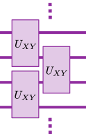
(a) $\mathfrak{a}_{1}(n)$

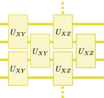
(b) $\mathfrak{a}_{9}(n)$

Figure 3: (a) Hamiltonian Variational Ansatz circuit for the Hamiltonian $H_{XY}=\sum_{i=1}^{n-1}X_{i}Y_{i+1}$, which parameterizes an element of the group $\mathrm{SO}(n)$. (b) Variational ansatz that parameterizes a unitary in $\mathrm{Sp}(2^{n-2})$ via products of unitaries generated by terms in $\mathfrak{a}_{9}(n)$.

We note that these types of brick-layer circuits also show up in the condensed matter physics literature on measurement-induced entanglement phase transitions [63, 64, 65], hence our classification may be of use in that context as well.

Example V.2.

Adapt-VQE. In ADAPT-VQE, one dynamically grows the circuit using a predetermined operator pool, so that each gate lowers the cost function by the largest amount [66]. This class of dynamical circuit ansätze can be understood as a Riemannian gradient flow over a specific subgroup [67]. This heuristic is popular in quantum chemistry for circuit design, where specific operator pools are considered that are tailored to fermionic Hamiltonians [68, 69, 70]. The operator pool can be seen as a set of generators, with a corresponding DLA. In the context of our classification, we can thus determine the resulting subgroup of the dynamically grown circuit ansatz based on the generators in the operator pool.

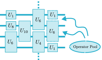
Figure 4: ADAPT-VQE circuit growing heuristic. We consider a generator pool in our classification and dynamically grow the circuit.

Example V.3.

Permutation-invariant circuits. Instead of a $1$-dimensional topology, one can consider a Hamiltonian with a fully connected topology (see Figure 5):

$$H=\sum_{1\leq i\neq j\leq n}A_{i}B_{j}.$$

This topology is common in ion trap quantum computers [71] and also shows up in the context of quantum Boltzmann machines [72, 73], which are the quantum equivalent of the Sherrington–Kirkpatrick model with tunable parameters [74]. Closely related are the so-called permutation-equivariant circuits, which consist of parameterized blocks of unitaries that are permutation invariant [75]. These circuit ansätze were shown to be powerful quantum machine learning models for permutation-invariant data sets. Our classification of permutation-invariant $2$-site Hamiltonians in one dimension thus provides a classification of DLAs for these types of ansätze.

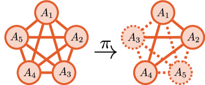
Figure 5: Permutation-invariant topology. Permuting sites leaves the Hamiltonian invariant.

V.2.2 Barren plateaus

A hurdle in minimizing a cost function of the form (6) are so-called barren plateaus [31], which are flat areas in the cost landscape of a variational quantum algorithm. When barren plateaus are present, the variance of gradients with respect to the gate parameters will decay, on average, exponentially as a function of system size. Hence, obtaining accurate estimates quickly becomes intractable due to the large number of shots required. There is a variety of different setups in which barren plateaus occur [29, 31, 32, 76, 77, 78, 79]. To mitigate this problem, several recent works are aimed at finding ways to avoid the regions where optimization is hard [80, 81, 82, 83, 84, 85, 86].

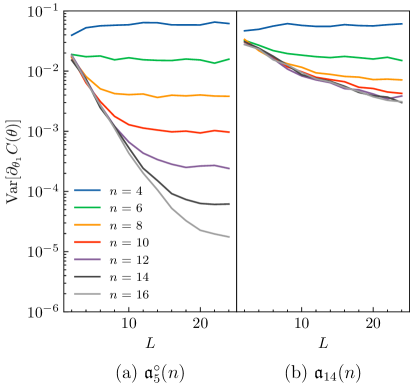
Figure 6: Barren plateaus in variational quantum circuits. We calculate the variance of $1000$ randomly initialized circuits with $\boldsymbol{\theta}$ sampled uniformly in $[0,\pi]$. (a) The Lie algebra $\mathfrak{a}_{5}^{\circ}(n)$ is isomorphic to $\mathfrak{so}(2^{n})$, $\mathfrak{so}(2^{n-2})^{\oplus 4}$ or $\mathfrak{sp}(2^{n-2})$ depending on $n$; hence we expect exponentially decaying gradients for all $n$. This is confirmed in the figure above, since for a linear increase in $n$, we see an order of magnitude decrease in the gradient variances. (b) Since $\mathfrak{a}_{14}(n)\cong\mathfrak{so}(2n)$, we find polynomially decaying gradients as a function of system size.

The relevance of our classification for barren plateaus stems from the conjecture of [30], which states that the variance of the gradients of gate parameters is inversely proportional to the dimension of the DLA $\mathfrak{g}$ of the circuit:

$$\mathrm{Var}[\partial_{k}C(\boldsymbol{\theta})]\in O\left(\frac{1}{\mathrm{poly}(\dim\mathfrak{g})}\right).$$

There are some subtleties involved in this conjecture, such as the locality of the cost function and the choice of initial state, which are discussed in [30]. In the common case where $H_{c}\in i\mathfrak{g}$, an exact formula for the variance was obtained independently in Refs. [87, 88], which in particular refines and proves the above conjecture. This formula was interpreted in Ref. [88] in terms of the $\mathfrak{g}$-purity [89, 90] of the initial state $\rho_{0}$ and the observable $H_{c}$, underscoring again the crucial role of the DLA.

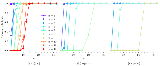
(a)

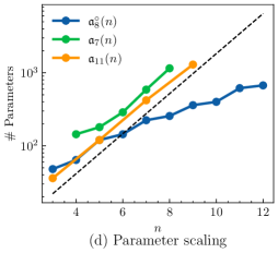
(b)

Figure 7: Overparameterization of variational quantum circuits. We plot the success probability of reaching a state with $|E_{0}-C(\boldsymbol{\theta})|<5\times 10^{-4}$ as a function of the circuit depth $L$, where $E_{0}$ is the lowest energy of the cost Hamiltonian $H_{c}$. These results were obtained by averaging $100$ random instances for each $L$ and $N$. The error bars indicate one standard deviation $\sigma$. A single random instance consists of $3000$ optimization steps of the Adam optimizer [91] with learning rate $\eta=10^{-2}$. A handful of instances converge to solutions that are further than $5\sigma$ from the mean and these outliers are therefore not included in the final plot. (a) The TFIM on a ring has DLA $\mathfrak{a}_{8}^{\circ}(n)\cong\mathfrak{so}(2n)^{\oplus 2}$, whose dimension scales quadratically. We see that for a moderate circuit depth, the probability of success goes to 1. (b) Since the DLA $\mathfrak{a}_{11}(n)\cong\mathfrak{so}(2^{n})$, we expect that overparameterization occurs at depths that are exponential in the system size. Although this is not immediately clear in here, we see in (d) that the number of parameters indeed scales exponentially in $n$. (c) For the Heisenberg chain, which has an exponentially-scaling DLA $\mathfrak{a}_{7}(n)$, the choice of initial state $\rho_{0}=|0\rangle\langle 0|^{\otimes n}$ prevents overparameterization from occurring for odd $n$. (d) If we set the threshold for overparameterization to be a success probability of $0.99$, we can plot the required number of parameters to reach this threshold. We see that $\mathfrak{a}_{11}(n)$ and $\mathfrak{a}_{7}(n)$ require an exponentially scaling number of parameters, whereas $\mathfrak{a}_{8}^{\circ}(n)$ only requires a polynomial number. The dashed line is a guiding line that indicates $O(4^{n})$ scaling.

As an illustration, we compare the barren plateau behavior for two of our Lie algebras, $\mathfrak{a}_{5}^{\circ}(n)$ and $\mathfrak{a}_{14}(n)$, whose dimensions scale exponentially and polynomially with $n$, respectively. We consider the cost function (6) with $H_{c}=Z_{1}Z_{2}$ and $\rho_{0}=|0\rangle\langle 0|^{\otimes n}$. The circuit ansatz $U(\boldsymbol{\theta})$ consists of unitaries generated by generators in our classification. To observe the barren plateau effect, we take the derivative of the cost function with respect to the first parameter in the first layer of the circuit, $\theta_{1}^{(1)}$. In Figure 6, we then observe the expected gradient decay as a function of the system size for an exponentially scaling DLA and a polynomially scaling DLA. In particular, in Figure 6(a) we consider the circuit generated by $H=\sum_{i=1}^{n-1}X_{i}Y_{i+1}+Y_{i}Z_{i+1}$ with periodic boundary conditions, whose DLA $\mathfrak{a}_{5}^{\circ}(n)$ is isomorphic to $\mathfrak{so}(2^{n})$, $\mathfrak{so}(2^{n-2})^{\oplus 4}$ or $\mathfrak{sp}(2^{n-2})$ depending on $n$ (see Theorem IV.2). Since $\dim\mathfrak{a}_{5}^{\circ}(n)=O(4^{n})$, we expect the gradients to decay exponentially. Similarly, in Figure 6(b) we consider the circuit generated by $\mathfrak{a}_{14}(n)\cong\mathfrak{so}(2n)$, which is described by the Hamiltonian $H=\sum_{i=1}^{n-1}X_{i}X_{i+1}+Y_{i}Y_{i+1}+X_{i}Y_{i+1}$. Here, we have $\dim\mathfrak{a}_{14}(n)=O(n^{2})$; hence, we expect the decay of gradients to be polynomial with respect to the system size.

According to Corollary IV.1, the only circuits free from barren plateaus generated by Hamiltonians in our classification, which are not composed of only $1$-qubit gates, have to be composed of $\mathfrak{so}(n)$-type, since these are the only polynomially scaling DLAs in our classification.

V.2.3 Overparameterization

Modern neural networks used in deep learning tend to have many more parameters than available data points, but are both easy to optimize and generalize well to unseen data in practice [92]. This phenomenon is known as overparameterization. In variational quantum computing, a similar effect has been observed [26, 27, 93], where deep variational quantum circuits tend to have favorable optimization properties. Recent works that have made progress in theoretically understanding this effect in quantum circuits can be connected to the DLA generated by the circuit ansätze used [29, 28]. In particular, in [29], the dimension of the DLA can be used to analyze the Hessian around the global minimum of a typical variational quantum eigensolver cost function [54]. Additionally, the authors find that the critical number of parameters needed to overparameterize a variational quantum circuit can be directly linked to the dimension of the associated DLA. In [28], the authors study the optimization dynamics of overparameterized quantum circuit as perturbations of Riemannian gradient flows [94]. The size of the DLA (defined as the effective dimension in [28]) allows one to bound the number of parameters required to reach the overparameterization regime.

Corollary IV.1 tells us that for quantum circuits constructed from the generators of $1$-dimensional spin chains, there are only DLAs whose dimension scales as $O(n)$, $O(n^{2})$ and $O(4^{n})$. Consequently, the linearly and quadratically scaling DLAs are expected to overparameterize with a non-exponential number of parameters. Additionally, the quadratically scaling DLAs in our classification correspond to free fermion models, whose dynamics can be simulated efficiently if $\rho_{0}$ is an eigenstate of $H_{c}$. However, choosing $\rho_{0}$ to be an arbitrary quantum state will still be intractable to simulate classically.

As discussed in [28], a requirement for overparameterzation is that the initial state has non-vanishing overlap with the ground state. Similarly, in [95], it is shown that choosing the initial state in the right symmetry sector is crucial for the quality of the optimization. We highlight this importance in one of the numerical examples, where we choose an initial state that prevents overparameterization from occurring for an odd number of sites.

In Figure 7, we illustrate the overparametrization phenomenon for three examples in our classification. In particular, in Figure 7(a), we consider the TFIM on a ring, which is given by the Hamiltonian $H_{c}=\sum_{i=1}^{n-1}Z_{i}Z_{i+1}+X_{i+1}$. The corresponding DLA is given by $\mathfrak{a}_{8}^{\circ}(n)\cong\mathfrak{so}(2n)^{\oplus 2}$, whose dimension scales quadratically in $n$. We take the Hamiltonian Variational Ansatz of $H_{c}$ on even and odd qubits as a circuit ansatz, and take the initial state to be $\rho_{0}=|+\rangle\langle+|^{\otimes n}$. We observe that the cost landscape quickly becomes favorable, resulting in almost guaranteed convergence to the lowest energy state.

In Figure 7(b), we take the DLA $\mathfrak{a}_{11}(n)\cong\mathfrak{so}(2^{n})$, and a Hamiltonian $H_{c}\in\mathfrak{so}(2^{n})$ given by a random orthogonal $2^{n}\times 2^{n}$ matrix. The circuit consists of unitaries generated by the generators of $\mathfrak{a}_{11}$ on even and odd qubits, and we take $\rho_{0}=|0\rangle\langle 0|^{\otimes n}$. It now takes much deeper circuits to reach the same success probabilities as in Figure 7(a), which is due to the exponential scaling of the DLA.

Finally, in Figure 7(c), we consider $\mathfrak{a}_{7}(n)$, which corresponds to the Heisenberg chain with $H_{c}=\sum_{i=1}^{n-1}X_{i}X_{i+1}+Y_{i}Y_{i+1}+Z_{i}Z_{i+1}$. The circuit is again the Hamiltonian Variational Ansatz of $H_{c}$, and $\rho_{0}=|0\rangle\langle 0|^{\otimes n}$. This choice of an initial state only works for an odd number $n$ of qubits, while it fails to produce the overparameterization phenomenon for even $n$, leading to a success probability of $0$ (not plotted). Instead, for even $n$, the optimization of deep circuits gets stuck in a local minimum. We still observe the exponential scaling of the number of parameters, in accordance with the scaling of the dimension of $\mathfrak{a}_{7}(n)$, which is $O(4^{n})$.

V.3 Relevance for spin systems

Our classification of Lie algebras arising in one dimension has significant bearing on a number of areas of physics and quantum simulation. The most direct connection is that we have established a set of models, some of which are traditional spin models [96, 97] studied in physics, while others are new (cf. Table S.II). The integrability [19, 98, 20], dynamical Lie algebra, and symmetry of $1$-dimensional spin systems remains an active area of research, and our result provides a database of models where desired properties can be selected or different hypotheses tested.

For example, models such as the XXZ chain and the TFIM model arise quite naturally from nearest-neighbor weight-$2$ Pauli strings, and are represented in our Lie algebras as $\mathfrak{a}_{7}(n)$ and $\mathfrak{a}_{8}(n)$, respectively. A key difference between these two models is that the TFIM is trivially integrable [98], while the XXZ model is more complex. This is reflected in the corresponding Lie algebras as well, as $\mathfrak{a}_{8}(n)\cong\mathfrak{so}(2n-1)$ (which scales polynomially in the number of qubits), and $\mathfrak{a}_{7}(n)\cong\mathfrak{su}(2^{n-1})$ (which scales exponentially). Interestingly, the number of polynomially-scaling algebras is relatively small ($\mathfrak{a}_{1},\mathfrak{a}_{2},\mathfrak{a}_{4},\mathfrak{a}_{8},\mathfrak{a}_{14},\mathfrak{a}^{\circ}_{1},\mathfrak{a}^{\circ}_{2},\mathfrak{a}^{\circ}_{4},\mathfrak{a}^{\circ}_{8},\mathfrak{a}^{\circ}_{14}$), and they are all of the $\mathfrak{so}$ type. The limited size of these algebras has been used to construct short- and/or fixed-depth circuits for state preparation [38] and time evolution [99, 100, 34, 35, 36] circuits.

The polynomially scaling algebras in principle come with a “maximal set of independent commuting quantum operators” [101], which enables the integration in the first place. Unfortunately, our method does not capture these because the conserved quantities are not single Pauli strings. However, global symmetries are preserved for some of the models; these include $\mathbb{Z}_{2}$ (spin flip), $\mathrm{SU}(2)$ (global spin rotation) and $\mathrm{U}(1)$ (global phase rotation).

One particular property of note is the presence of non-commuting charges—that is, elements of the stabilizer that do not commute. These are found in $\mathfrak{a}_{8}(n),\mathfrak{a}_{9}(n)$ for all $n$, and in $\mathfrak{a}_{2}(n){-}\mathfrak{a}_{7}(n),\mathfrak{a}_{10}(n)$ for odd $n$ only. Non-commuting charges give rise to a wide range of quantum effects in thermodynamics (see Ref. [39] for a review). Notably, the presence of non-commuting charges complicates questions regarding thermalization. Depending on the context, they either help thermalization (e.g. by increasing entanglement entropy [102]) or hinder it (e.g. by invalidating the Eigenstate Thermalization Hypothesis [103]). Although these effects have been primarily observed when the non-commuting charges are extensive, and the ones discussed here are intensive, our framework could be extended to the former as well. Perhaps more interestingly within the context of quantum computing, non-commuting charges couple the dynamics between different irreducible representations of the charges, severely limiting the unitaries that can be implemented [104].

A final point is the appearance of symplectic Lie algebras, which are not as common as the orthogonal or unitary types. Here they appear from an AIII Cartan decomposition of a larger Lie algebra; in applications, they come up in the preparation of bosonic quantum states [47], photonics [105] and Clifford circuits/error correction [106].

VI Conclusion

We have provided a classification of the dynamical Lie algebras (DLA) of $2$-local spin systems with open, periodic or permutation invariant topology in one dimension, and have discussed the relevance of this result in a variety of contexts. We have discovered several new examples beyond the standard Ising and Heisenberg models; thus increasing dramatically the number of explicit Hamiltonians available for theoretical investigations. It would be interesting to study in more detail the thermodynamic properties of these new Hamiltonians, and in particular to determine all of their symmetries, including the extensive non-commuting charges. We hope that our classification can be used to inspire new quantum algorithms and allow researchers to identify the circuits that they use in practice with the Lie algebras in our classification. Moreover, the methods that we have developed can be used to identify the DLA even in cases that fall outside of our classification.

One possible extension of our results would be to consider other topologies, such as $2$- and $3$-dimensional graphs. The challenge is that the number of possible Hamiltonians might become intractable. We would have to add more constraints to the Hamiltonians we consider, in order to reduce the size of the power set, or come up with alternative approaches to enumerate all unique DLAs.

Another future direction would be to consider other types of systems. For example, instead of spin systems, we could consider fermionic or bosonic Hamiltonians. Such a classification already exists for nearest-neighbor interactions on cubic lattices [47, 107], so this question would have to be explored in the context of non-cubic graphs.

Author Contributions

The project was conceived by RW and BNB. Computer calculations and numerical simulations were performed by RW, with some assistance from AFK. Mathematical theorems were derived by BNB with the assistance of EK. The main part of the manuscript was written mostly by RW, while the Supplemental Materials were written by BNB. The figures were made by RW, and the tables by AFK and EK (except Table S.I by BNB). All authors contributed to reviewing and editing the manuscript.

Data Availability

Data generated and analyzed during the current study are available at [43].

Competing Interests

The authors declare no competing interests.

Supplemental Material

A Preliminaries on Pauli strings and $\mathfrak{su}(2^{n})$

Length-$n$ Pauli strings, when multiplied with the imaginary unit $i$, form a natural basis for the Lie algebra $\mathfrak{u}(2^{n})$ of skew-Hermitian matrices. Because of this and their other remarkable properties, Pauli strings have been excessively used in this and many other works. In this section, we review the notation and basic properties of Pauli strings, the Lie algebra $\mathfrak{su}(2^{n})$, and its subalgebras $\mathfrak{so}(2^{n})$ and $\mathfrak{sp}(2^{n-1})$. We also discuss involutions of Lie algebras, and particularly of $\mathfrak{su}(2^{n})$.

I Pauli strings

Throughout the paper, we work with the Pauli matrices

$$\sigma_{0}=I=\begin{pmatrix}1&0\\ 0&1\end{pmatrix},\qquad\sigma_{1}=X=\begin{pmatrix}0&1\\ 1&0\end{pmatrix},\qquad\sigma_{2}=Y=\begin{pmatrix}0&-i\\ i&0\end{pmatrix},\qquad\sigma_{3}=Z=\begin{pmatrix}1&0\\ 0&-1\end{pmatrix},$$

including the identity matrix $I$, which form a basis for the real vector space of $2\times 2$ Hermitian matrices. We will denote by $A^{T}$ the transpose of a matrix, and by $A^{\dagger}$ its Hermitian conjugate (which is obtained from $A^{T}$ by taking complex conjugates of all entries). Thus, $A^{\dagger}=A$ for all $A\in\mathcal{P}_{1}:=\{I,X,Y,Z\}$. On the other hand, we have

$$Y^{T}=-Y,\qquad A^{T}=A\quad\text{for}\quad A=I,X,Z.$$

Fix a positive number $n$. Length-$n$ Pauli strings are tensor products of $n$ Pauli matrices of the form

$$a=A^{1}\otimes A^{2}\otimes\dots\otimes A^{n},\qquad A^{j}\in\mathcal{P}_{1}$$ (A1)

(where the superscripts are indices not powers). We denote the set of all such Pauli strings by $\mathcal{P}_{n}:=\{I,X,Y,Z\}^{\otimes n}$. Every $a\in\mathcal{P}_{n}$ is a linear operator on the Hilbert space $(\mathbb{C}^{2})^{\otimes n}$ of $n$ qubits, so $a$ can be represented as a matrix of size $2^{n}\times 2^{n}$ (by the Kronecker product). In particular, $I^{\otimes n}$ is the $2^{n}\times 2^{n}$ identity matrix. The Hermitian conjugate and transpose of a Pauli string are done componentwise:

$$a^{\dagger} =(A^{1})^{\dagger}\otimes(A^{2})^{\dagger}\otimes\dots\otimes(A^{n})^{\dagger}=a,$$

$$a^{T} =(A^{1})^{T}\otimes(A^{2})^{T}\otimes\dots\otimes(A^{n})^{T}=(-1)^{\#\{A^{j}=Y\}}a.$$

All Pauli strings are Hermitian, and $\mathcal{P}_{n}$ is a basis (over $\mathbb{R}$) of the vector space of $2^{n}\times 2^{n}$ Hermitian matrices.

To shorten the notation, we will often omit the tensor product signs in Pauli strings, so (A1) will be written as $a=A^{1}A^{2}\cdots A^{n}$. For example, we will write

$$XX=X\otimes X,\qquad XY=X\otimes Y,\qquad Z\cdots Z=Z^{\otimes n},\quad\text{etc.}$$

For $A\in\mathcal{P}_{1}$ and $1\leq j\leq n$, we will denote by

$$A_{j}:=I^{\otimes(j-1)}\otimes A\otimes I^{\otimes(n-j)}$$ (A2)

the linear operator $A$ acting on the $j$-th qubit. For example, for $n=3$,

$$X_{1}=XII=X\otimes I\otimes I,\qquad Z_{2}=IZI=I\otimes Z\otimes I,\qquad X_{1}Z_{2}Y_{3}=XZY=X\otimes Z\otimes Y,\quad\text{etc.}$$

With this notation, we distinguish

$$A_{1}A_{2}\cdots A_{n}=AA\cdots A=A\otimes A\otimes\cdots\otimes A=A^{\otimes n}$$

from (A1), where in the latter the tensor factors $A^{1},\dots,A^{n}$ are allowed to be different.

When there is a danger to confuse the tensor product and the matrix product, we will use $\cdot$ for the product of matrices. We have:

$$X\cdot Y=iZ=-Y\cdot X,\qquad Y\cdot Z=iX=-Z\cdot Y,\qquad Z\cdot X=iY=-X\cdot Z,$$

and each Pauli matrix squares to the identity:

$$X\cdot X=Y\cdot Y=Z\cdot Z=I.$$

The matrix product of Pauli strings is done componentwise:

$$(A^{1}\otimes\dots\otimes A^{n})\cdot(B^{1}\otimes\dots\otimes B^{n})=(A^{1}\cdot B^{1})\otimes\dots\otimes(A^{n}\cdot B^{n}).$$

From here, it is easy to deduce the following important properties of Pauli strings.

Lemma A.1.

For any $a,b\in\mathcal{P}_{n}$, we have $a\cdot a=I^{\otimes n}$ and $a\cdot b=\pm b\cdot a$. Hence, any two Pauli strings either commute or anticommute.

Notice that the product of two Pauli strings is again a Pauli string, up to a multiple of $\pm 1,\pm i$. Thus, the set $\{\pm a,\pm ia\,|\,a\in\mathcal{P}_{n}\}$ is a group under the matrix product, called the Pauli group. The following corollary of Lemma A.1 will be useful in the future.

Corollary A.1.

For any $a,b\in\mathcal{P}_{n}$, if $[a,b]:=a\cdot b-b\cdot a\neq 0$, then $[a,[a,b]]=4b$.

Proof.

When $[a,b]\neq 0$, we have $[a,b]=2a\cdot b$ and $[a,[a,b]]=4a\cdot a\cdot b=4b$. ∎

Another important consequence of Lemma A.1 is Euler’s formula

$$e^{i\theta a}=(\cos\theta)I^{\otimes n}+i(\sin\theta)a,\qquad a\in\mathcal{P}_{n},\;\;\theta\in\mathbb{R}.$$ (A3)

A useful special case is $\theta=\pi/2$; then

$$e^{i\frac{\pi}{2}a}=ia,\qquad a\in\mathcal{P}_{n}.$$ (A4)

Note that any $a\in\mathcal{P}_{n}$ is Hermitian (i.e., $a^{\dagger}=a$), $ia$ is skew-Hermitian (i.e., $(ia)^{\dagger}=-ia$), and $U=e^{i\theta a}$ is unitary (i.e., $UU^{\dagger}=I^{\otimes n}$). In the following, we will use the following corollary of Euler’s formulas (A3), (A4).

Corollary A.2.

For any anticommuting $a,b\in\mathcal{P}_{n}$ and a real number $\theta$, we have

$$e^{i\theta a}\cdot b=b\cdot e^{-i\theta a}.$$ (A5)

In particular,

$$e^{i\frac{\pi}{4}a}\,b\,e^{-i\frac{\pi}{4}a}=ia\cdot b.$$ (A6)

II The Lie algebras $\mathfrak{su}(N)$, $\mathfrak{so}(N)$, and $\mathfrak{sp}(N)$

The purpose of this subsection is to review some standard terminology concerning Lie algebras, especially $\mathfrak{su}(N)$, $\mathfrak{so}(N)$, and $\mathfrak{sp}(N)$. We fix a positive integer $N$; later we will have $N=2^{n}$ where $n$ is the number of qubits.

The set $\mathbb{C}^{N\times N}$ of $N\times N$ matrices with complex entries is a vector space over $\mathbb{C}$, as matrices can be added or multiplied by complex scalars. Then $\mathbb{C}^{N\times N}$ is an associative algebra under the matrix product $ab$, i.e., $ab$ is bilinear (depends linearly on both $a$ or $b$) and associative: $a(bc)=(ab)c$. Under the commutator bracket $[a,b]=ab-ba$, we get a complex Lie algebra denoted as $\mathfrak{gl}(N,\mathbb{C})$.

In general, a Lie algebra is defined as a vector space $\mathfrak{g}$ (over $\mathbb{C}$), equipped with a bilinear operation $[a,b]\in\mathfrak{g}$ for $a,b\in\mathfrak{g}$, which satisfies the following skew-symmetry and Jacobi identity:

$$[a,b]=-[b,a],\qquad[a,[b,c]]=[[a,b],c]+[b,[a,c]].$$

It is convenient to use the notation $\mathrm{ad}_{a}(b):=[a,b]$ for $a,b\in\mathfrak{g}$. Then $\mathrm{ad}_{a}$ is a linear operator on $\mathfrak{g}$ for every $a\in\mathfrak{g}$. A trivial example of a Lie algebra is any vector space $\mathfrak{g}$ with the zero bracket $[a,b]=0$ for all $a,b\in\mathfrak{g}$; such Lie algebras are called Abelian.

A subalgebra $\mathfrak{s}$ of a Lie algebra $\mathfrak{g}$ is a subspace (i.e., closed under vector addition and scalar multiplication), which is also closed under the bracket: $a,b\in\mathfrak{s}$ $\Rightarrow$ $[a,b]\in\mathfrak{s}$. For example, the set $\mathfrak{sl}(N,\mathbb{C})$ of all $N\times N$ complex matrices with trace $0$ is a subalgebra of $\mathfrak{gl}(N,\mathbb{C})$; hence, it is itself a Lie algebra. Recall that an ideal in a Lie algebra $\mathfrak{g}$ is a subspace $\mathfrak{s}$ such that $a\in\mathfrak{g}$, $b\in\mathfrak{s}$ $\Rightarrow$ $[a,b]\in\mathfrak{s}$. For example, both $\mathfrak{sl}(N,\mathbb{C})$ and $\mathbb{C}I_{N}$ (where $I_{N}$ is the $N\times N$ identity matrix) are ideals of $\mathfrak{gl}(N,\mathbb{C})$, and

$$\mathfrak{gl}(N,\mathbb{C})=\mathfrak{sl}(N,\mathbb{C})\oplus\mathbb{C}I_{N}$$

is a direct sum of not just subspaces but of commuting subalgebras and ideals. When we write a direct sum of Lie algebras, we will always mean that the summands are subalgebras that commute with each other. The space $\mathbb{C}I_{N}$ is the center $Z(\mathfrak{g})$ of $\mathfrak{g}=\mathfrak{gl}(N,\mathbb{C})$, i.e., the set of all $c\in\mathfrak{g}$ such that $[c,a]=0$ for all $a\in\mathfrak{g}$.

The Lie algebra $\mathfrak{sl}(N,\mathbb{C})$ is simple, which means that it is not Abelian and has no ideals other than the trivial $\{0\}$ and the whole algebra. Other examples of simple Lie algebras over $\mathbb{C}$ are provided by the orthogonal Lie algebras $\mathfrak{so}(N,\mathbb{C})$ and the symplectic Lie algebras $\mathfrak{sp}(2N,\mathbb{C})$. Let us recall that $\mathfrak{so}(N,\mathbb{C})$ is defined as the set of all complex skew-symmetric matrices (i.e., such that $a^{T}=-a$), and it is a subalgebra of $\mathfrak{sl}(N,\mathbb{C})$. Consider the $2N\times 2N$ matrix

$$J_{2N}:=\begin{pmatrix}0&I_{N}\\ -I_{N}&0\end{pmatrix}.$$

Then $\mathfrak{sp}(2N,\mathbb{C})$ is defined as the set of all $a\in\mathfrak{gl}(2N,\mathbb{C})$ such that $a^{T}J_{2N}=-J_{2N}a$; this is a subalgebra of $\mathfrak{sl}(2N,\mathbb{C})$.

In this paper, we will work with Lie algebras over $\mathbb{R}$. The set of all skew-Hermitian matrices (i.e., satisfying $a^{\dagger}=-a$) is a real vector space, and is closed under the commutator; hence, it is a real Lie algebra, denoted $\mathfrak{u}(N)$. Imposing that the trace of the matrix is $0$, we get the Lie algebra $\mathfrak{su}(N)$. If a matrix has real entries, then it is skew-Hermitian if and only if it is skew-symmetric. Thus, we have the subalgebra

$$\mathfrak{so}(N):=\mathfrak{so}(N,\mathbb{R})=\bigl{\{}a\in\mathfrak{su}(N)\,\big{|}\,a^{T}=-a\bigr{\}}\subset\mathfrak{su}(N).$$ (A7)

On the other hand, the Lie algebra of real symplectic matrices $\mathfrak{sp}(2N,\mathbb{R})$ is not a subalgebra of $\mathfrak{su}(2N)$. Instead of it, the relevant subalgebra is

$$\mathfrak{sp}(N):=\mathfrak{sp}(2N,\mathbb{C})\cap\mathfrak{su}(2N)=\bigl{\{}a\in\mathfrak{su}(2N)\,\big{|}\,a^{T}J_{2N}=-J_{2N}a\bigr{\}}\subset\mathfrak{su}(2N).$$ (A8)

The Lie algebras $\mathfrak{su}(N)$, $\mathfrak{so}(N)$, $\mathfrak{sp}(N)$ are simple and compact (they are Lie algebras of compact Lie groups). Their dimensions over $\mathbb{R}$ are given by:

$$\dim\mathfrak{su}(N)=N^{2}-1,\qquad\dim\mathfrak{so}(N)=\frac{1}{2}N(N-1),\qquad\dim\mathfrak{sp}(N)=N(2N+1).$$ (A9)

It is known (see e.g. [25, 40]) that any subalgebra of $\mathfrak{u}(N)$ is either Abelian or a direct sum of a center (which could be $\{0\}$) and Lie algebras isomorphic to one of $\mathfrak{su}$, $\mathfrak{so}$, $\mathfrak{sp}$ or to one of five exceptional compact simple Lie algebras (cf. Proposition I.1). For completeness, we provide the proof of this important fact here.

Proposition A.1.

Any subalgebra of $\mathfrak{u}(N)$ is either Abelian or a direct sum of compact simple Lie algebras and a center.

Proof.

First, recall that the trace form $(a,b)=\mathrm{Tr}[ab]$ is negative definite on $\mathfrak{u}(N)$. Indeed, one can see that

$$\mathrm{Tr}[H^{2}]=\sum_{j=1}^{N}\lambda_{j}^{2}>0$$

for any nonzero Hermitian matrix $H\in i\mathfrak{u}(N)$ with eigenvalues $\lambda_{1},\dots,\lambda_{N}$, because all $\lambda_{j}$ are real. Second, the trace form $(\cdot,\cdot)$ is bilinear, symmetric and invariant; the latter meaning that

$$([a,b],c)=-(b,[a,c]),\qquad a,b,c\in\mathfrak{u}(N).$$

All of these follow easily from the properties of the trace.

Now let $\mathfrak{g}$ be a subalgebra of $\mathfrak{u}(N)$. Then the same proof as in [108], Corollary 4.25, shows that $\mathfrak{g}$ is reductive, i.e., it is a direct sum of simple or Abelian ideals. Indeed, for any ideal $\mathfrak{s}$ of $\mathfrak{g}$, we have an orthogonal direct sum

$$\mathfrak{g}=\mathfrak{s}\oplus\mathfrak{s}^{\perp},$$

due to the definiteness of the trace form. Furthermore, the invariance of the trace form implies that $\mathfrak{s}^{\perp}$ is itself an ideal of $\mathfrak{g}$. As both $\mathfrak{s}$ and $\mathfrak{s}^{\perp}$ are ideals, they must commute: $[\mathfrak{s},\mathfrak{s}^{\perp}]\subseteq\mathfrak{s}\cap\mathfrak{s}^{\perp}=\{0\}$. Thus, $\mathfrak{g}$ is a direct sum of commuting ideals. Suppose that $\dim\mathfrak{s}>1$ and $\mathfrak{s}$ is not simple as a Lie algebra. Then $\mathfrak{s}$ has a nonzero proper ideal $\mathfrak{t}$. From $[\mathfrak{t},\mathfrak{s}]\subseteq\mathfrak{t}$ and $[\mathfrak{t},\mathfrak{s}^{\perp}]=\{0\}$, we get that $[\mathfrak{t},\mathfrak{g}]\subseteq\mathfrak{t}$, so $\mathfrak{t}$ is an ideal of $\mathfrak{g}$. Hence, we can proceed by induction on $\dim\mathfrak{g}$ and break $\mathfrak{g}$ into a direct sum of commuting ideals, each of which is either simple or $1$-dimensional (Abelian).

Finally, we note that any simple subalgebra $\mathfrak{g}$ of $\mathfrak{u}(N)$ is compact, i.e., the Lie group $e^{\mathfrak{g}}$ is compact as a closed subgroup of the compact Lie group $\mathrm{U}(N)$ (see e.g. [108], Proposition 4.27, whose proof still applies). The classification of all compact simple Lie algebras is due to Cartan, and can be found in standard textbooks; for example in [108], Chapter VI. ∎

Let now $N=2^{n}$ where $n$ is the number of qubits. Then a basis for $\mathfrak{u}(2^{n})$ is given by $i\mathcal{P}_{n}$ (see Sect. I). To get a basis for $\mathfrak{su}(2^{n})$, we just have to remove $iI^{\otimes n}$, since $I^{\otimes n}=I_{N}$ is the identity matrix. A basis for $\mathfrak{so}(2^{n})$ consists of all $ia$ where $a\in\mathcal{P}_{n}$ is a Pauli string containing an odd number of $Y$’s. Finally, to describe the subalgebra $\mathfrak{sp}(2^{n-1})\subset\mathfrak{su}(2^{n})$, we observe that

$$Y_{1}=Y\otimes I^{\otimes(n-1)}=-i\begin{pmatrix}0&I_{\frac{N}{2}}\\ -I_{\frac{N}{2}}&0\end{pmatrix}=-iJ_{N}.$$

Therefore,

$$\mathfrak{sp}(2^{n-1})=\bigl{\{}a\in\mathfrak{su}(2^{n})\,\big{|}\,a^{T}\cdot Y_{1}=-Y_{1}\cdot a\bigr{\}}.$$ (A10)

The following definition plays a crucial role throughout the paper.

Definition A.1.

For a Lie algebra $\mathfrak{g}$ and a subset $\mathcal{A}\subset\mathfrak{g}$, we define $\langle\mathcal{A}\rangle_{\mathrm{Lie}}$ to be the minimal (under inclusion) subalgebra of $\mathfrak{g}$ that contains $\mathcal{A}$. We say that $\langle\mathcal{A}\rangle_{\mathrm{Lie}}$ is the subalgebra generated by $\mathcal{A}$, and that $\mathcal{A}$ is a set of generators of $\langle\mathcal{A}\rangle_{\mathrm{Lie}}$. In the case when $\mathcal{A}\subset\mathcal{P}_{n}$ is a set of Pauli strings, we will slightly abuse the notation and write $\langle\mathcal{A}\rangle_{\mathrm{Lie}}$ for the subalgebra of $\mathfrak{su}(2^{n})$ generated by the subset $i\mathcal{A}\subset\mathfrak{su}(2^{n})$.

More explicitly, it follows from the Jacobi identity that $\langle\mathcal{A}\rangle_{\mathrm{Lie}}$ is the set of all linear combinations of all nested commutators of the form

$$\mathrm{ad}_{a_{1}}\mathrm{ad}_{a_{2}}\cdots\mathrm{ad}_{a_{r}}(a_{r+1})=[a_{1},[a_{2},[\cdots[a_{r},a_{r+1}]\cdots]]],\qquad a_{j}\in\mathcal{A},\;\;r\geq 0,$$ (A11)

where $r=0$ corresponds to an empty commutator $=a_{1}$. The following simple observation will be useful.

Lemma A.2.

For any subset $\mathcal{A}\subset\mathcal{P}_{n}$, the Lie algebra $\langle\mathcal{A}\rangle_{\mathrm{Lie}}\subseteq\mathfrak{su}(2^{n})$ generated by $i\mathcal{A}$ has a basis consisting of Pauli strings times $i$. In other words,

$$\langle\mathcal{A}\rangle_{\mathrm{Lie}}=\mathrm{span}_{\mathbb{R}}\bigl{(}i\mathcal{P}_{n}\cap\langle\mathcal{A}\rangle_{\mathrm{Lie}}\bigr{)}.$$

Proof.

By definition, $\langle\mathcal{A}\rangle_{\mathrm{Lie}}$ is linearly spanned over $\mathbb{R}$ by all elements of the form (A11) with $a_{j}\in i\mathcal{A}\subset i\mathcal{P}_{n}$. All such elements are scalar multiples of Pauli strings, i.e., lie in $i\mathbb{R}\mathcal{P}_{n}$. From any spanning set, one can choose a subset that forms a basis. ∎

III Involutions of $\mathfrak{su}(2^{n})$

In this subsection, we explain how we can describe subalgebras of $\mathfrak{su}(2^{n})$ as fixed points of involutions. We start more generally by recalling that an isomorphism from a Lie algebra $\mathfrak{g}$ to another Lie algebra $\mathfrak{g}_{1}$ is an invertible linear transformation $\varphi\colon\mathfrak{g}\to\mathfrak{g}_{1}$ that is compatible with the bracket, i.e., $\varphi([a,b])=[\varphi(a),\varphi(b)]$ for all $a,b\in\mathfrak{g}$. We write $\mathfrak{g}\cong\mathfrak{g}_{1}$ to indicate that $\mathfrak{g}$ is isomorphic to $\mathfrak{g}_{1}$. An automorphism of $\mathfrak{g}$ is an isomorphism $\varphi\colon\mathfrak{g}\to\mathfrak{g}$. The set of fixed points of $\varphi$ is defined as:

$$\mathfrak{g}^{\varphi}=\bigl{\{}a\in\mathfrak{g}\,\big{|}\,\varphi(a)=a\bigr{\}}.$$ (A12)

It is easy to check that $\mathfrak{g}^{\varphi}$ is a subalgebra of $\mathfrak{g}$, called the fixed-point subalgebra. An involution on $\mathfrak{g}$ is an automorphism $\theta\colon\mathfrak{g}\to\mathfrak{g}$ with the property that $\theta(\theta(a))=a$ for all $a\in\mathfrak{g}$, i.e., $\theta^{-1}=\theta$.

Later, we will need to understand how, for an involution $\theta$, the fixed-point subalgebra $\mathfrak{g}^{\theta}$ transforms under another automorphism $\varphi$ of $\mathfrak{g}$. The answer is given in the following lemma.

Lemma A.3.

Let $\varphi$ be an automorphism of a Lie algebra $\mathfrak{g}$, and $\theta$ be an involution of $\mathfrak{g}$. Then $\varphi\theta\varphi^{-1}$ is an involution of $\mathfrak{g}$, and we have $\varphi(\mathfrak{g}^{\theta})=\mathfrak{g}^{\varphi\theta\varphi^{-1}}$.

Proof.

Note that $\varphi\theta\varphi^{-1}$ is an automorphism of $\mathfrak{g}$, since the composition of isomorphisms is again an isomorphism. It is an involution of $\mathfrak{g}$, because $(\varphi\theta\varphi^{-1})^{-1}=\varphi\theta^{-1}\varphi^{-1}=\varphi\theta\varphi^{-1}$. To check the claim about the fixed points, suppose that $a\in\mathfrak{g}^{\theta}$, i.e., $\theta(a)=a$. Then

$$(\varphi\theta\varphi^{-1})\varphi(a)=\varphi(\theta(a))=\varphi(a)\;\;\Rightarrow\;\;\varphi(a)\in\mathfrak{g}^{\varphi\theta\varphi^{-1}}.$$

Conversely, if $b\in\mathfrak{g}^{\varphi\theta\varphi^{-1}}$, then the above calculation shows that $a=\varphi^{-1}(b)\in\mathfrak{g}^{\theta}$. ∎

Now we will discuss how to construct automorphisms and involutions of $\mathfrak{su}(N)$.

Lemma A.4.

Suppose that $U$ and $Q$ are unitary $N\times N$ matrices, and $Q^{T}=\pm Q$. Then the formulas

$$\varphi(a)=UaU^{\dagger},\qquad\theta(a)=-Qa^{T}Q^{\dagger},\qquad a\in\mathfrak{su}(N),$$

define an automorphism $\varphi$ and an involution $\theta$ of $\mathfrak{su}(N)$. Moreover, we have

$$(\varphi\theta\varphi^{-1})(a)=-(UQU^{T})a^{T}(UQU^{T})^{\dagger},\qquad a\in\mathfrak{su}(N).$$

Proof.

First, note that $\varphi$ is invertible with $\varphi^{-1}(a)=U^{\dagger}aU$. It is clear that $\varphi([a,b])=[\varphi(a),\varphi(b)]$, because

$$\varphi(a)\varphi(b)=UaU^{\dagger}UbU^{\dagger}=UabU^{\dagger}=\varphi(ab)$$

for any two matrices $a,b$. (This means that $\varphi$ is an automorphism of the associative algebra $\mathbb{C}^{N\times N}$.)

To check that $\theta$ is an involution, we calculate

$$\theta(\theta(a))=\theta(-Qa^{T}Q^{\dagger})=Q(Q^{\dagger})^{T}(a^{T})^{T}Q^{T}Q^{\dagger}=Q(\pm Q^{\dagger})a(\pm Q)Q^{\dagger}=a,$$

where we used that $(Q^{\dagger})^{T}=(Q^{T})^{\dagger}$. Next, we have

$$\theta(ab)=-Q(ab)^{T}Q^{\dagger}=-Qb^{T}a^{T}Q^{\dagger}=-Qb^{T}Q^{\dagger}Qa^{T}Q^{\dagger}=-\theta(b)\theta(a).$$

This implies that $\theta([a,b])=[\theta(a),\theta(b)]$ and proves that $\theta$ is an involution of $\mathfrak{su}(N)$.

Finally, we find

$$(\varphi\theta\varphi^{-1})(a) =\varphi\bigl{(}\theta(U^{\dagger}aU)\bigr{)}$$

$$=-\varphi\bigl{(}QU^{T}a^{T}(U^{\dagger})^{T}Q^{\dagger}\bigr{)}$$

$$=-UQU^{T}a^{T}(U^{\dagger})^{T}Q^{\dagger}U^{\dagger}$$

$$=-(UQU^{T})a^{T}(UQU^{T})^{\dagger},$$

as claimed. ∎

Example A.1.

The subalgebra $\mathfrak{so}(N)\subset\mathfrak{su}(N)$ is the fixed-point subalgebra of the involution $a\mapsto-a^{T}$ (see (A7)). Similarly, we see from (A8) that $\mathfrak{sp}(N)=\mathfrak{su}(2N)^{\theta}$, where $\theta(a)=-Qa^{T}Q^{\dagger}$ as in Lemma A.4, with $Q=-iJ_{2N}$.

It is well known, in general, that for an involution $\theta(a)=-Qa^{T}Q^{\dagger}$ as in Lemma A.4, the fixed-point subalgebra $\mathfrak{su}(N)^{\theta}\cong\mathfrak{so}(N)$ when $Q^{T}=Q$, and $\mathfrak{su}(N)^{\theta}\cong\mathfrak{sp}(N/2)$ when $Q^{T}=-Q$ (in which case $N$ must be even). For completeness, we will present the proof of these facts in the special case of interest to us: when $N=2^{n}$ and $Q\in\mathcal{P}_{n}$ is a length-$n$ Pauli string. Note that all Pauli strings $Q$ satisfy $Q=Q^{\dagger}=Q^{-1}$ and $Q^{T}=\pm Q$.

Lemma A.5.

For any Pauli string $Q\in\mathcal{P}_{n}$, there exists a unitary $2^{n}\times 2^{n}$ matrix $U$ such that

$$UQU^{T}=\begin{cases}I^{\otimes n},&\text{if}\;\;Q^{T}=Q,\\ Y_{1},&\text{if}\;\;Q^{T}=-Q.\end{cases}$$

Proof.

In the case $Q^{T}=Q$, we let $U=e^{i\frac{\pi}{4}Q}$. Then

$$UQU^{T}=UQU=U^{2}Q=e^{i\frac{\pi}{2}Q}Q=iQ\cdot Q=iI^{\otimes n},$$

where we used Euler’s formula (A4). The superfluous phase $i$ can be eliminated by applying the unitary transformation $V=e^{-i\frac{\pi}{4}I^{\otimes n}}$, which satisfies $V^{T}=V$ and $V^{2}=-iI^{\otimes n}$.

Suppose now that $Q^{T}=-Q$, which means that $Q$ contains an odd number of $Y$’s. If $Q$ has a $Y$ in $j$-th position, let $P=Y_{j}\cdot Q$ and $U=e^{i\frac{\pi}{4}P}$. Note that

$$P=Y_{j}\cdot Q=Q\cdot Y_{j}\;\;\Rightarrow\;\;P\cdot Q=Q\cdot P=Y_{j}$$

and

$$P^{T}=Q^{T}\cdot Y_{j}^{T}=(-Q)\cdot(-Y_{j})=Q\cdot Y_{j}=P.$$

Hence, as above, we find:

$$UQU^{T}=UQU=U^{2}Q=e^{i\frac{\pi}{2}P}Q=iP\cdot Q=iY_{j}.$$

If $j=1$, we are done (after eliminating the phase $i$). If $j\neq 1$, we apply the unitary transformation $e^{-i\frac{\pi}{4}Y_{1}Y_{j}}$ and obtain:

$$e^{-i\frac{\pi}{4}Y_{1}Y_{j}}(iY_{j})(e^{-i\frac{\pi}{4}Y_{1}Y_{j}})^{T}=e^{-i\frac{\pi}{2}Y_{1}Y_{j}}(iY_{j})=-iY_{1}Y_{j}\cdot(iY_{j})=Y_{1},$$

completing the proof. ∎

Corollary A.3.

Any Pauli string $Q\in\mathcal{P}_{n}$ defines an involution $\theta$ of $\mathfrak{su}(2^{n})$ given by $\theta(a)=-Qa^{T}Q$. The fixed-point subalgebra of this involution is:

$$\mathfrak{su}(2^{n})^{\theta}\cong\begin{cases}\mathfrak{so}(2^{n}),&\text{if}\;\;Q^{T}=Q,\\ \mathfrak{sp}(2^{n-1}),&\text{if}\;\;Q^{T}=-Q.\end{cases}$$

B Statement of Results

I Subalgebras of $\mathfrak{su}(4)$ up to symmetry

Recall that $\mathfrak{su}(4)$ has a basis over $\mathbb{R}$ consisting of all possible tensor products $iAB$, where $A,B\in\{I,X,Y,Z\}$, $AB\neq II$. As a first step, we found that there are $202$ subalgebras of $\mathfrak{su}(4)$, which are generated by subsets of this basis. The symmetry group $S_{3}\times\mathbb{Z}_{2}$ acts on $\mathfrak{su}(4)$ as follows: the symmetric group $S_{3}$ permutes simultaneously all $\{X,Y,Z\}$, while the non-identity element of $\mathbb{Z}_{2}$ acts as the flip $AB\rightleftharpoons BA$. We examined the orbits of the action of $S_{3}\times\mathbb{Z}_{2}$ on the $202$ subalgebras, and found that there are $36$ orbits, which are listed in Table S.I below. The full list of all $202$ subalgebras is presented in the next subsection.

The numbers $s,p,e,d$ are equal to the numbers of: single Paulis (such as $XI$), single Pauli pairs (such as $XI,IX$), double equal Paulis (such as $XX$), and double different Paulis (such as $XY$), respectively, in the basis of the subalgebra. These are invariant under the action of the symmetry group; hence, subalgebras of $\mathfrak{su}(4)$ with different invariants are not equivalent to each other. It turns out that the only two non-equivalent subalgebras with the same invariants are $\mathfrak{a}_{2}$ and $\mathfrak{a}_{5}$.

We distinguish between three types of subalgebras. The $\mathfrak{a}$-type Lie algebras are generated by products of two Paulis both different from the identity, whereas the $\mathfrak{b}$-type can be generated by Pauli strings that contain the identity. The $\mathfrak{c}$-type Lie algebras are an edge case where the generators contain some Pauli strings of the form $a\otimes I$ without the corresponding term $I\otimes a$. These Lie algebras will behave like the $\mathfrak{b}$-type Lie algebras but include a boundary effect at the last site in the chain. In particular, note that all single Pauli generators come in pairs such as $XI,IX$ or $YI,IY$ or $ZI,IZ$ due to the translation invariance; hence we exclude the Lie algebras $\mathfrak{c}_{0},\dots,\mathfrak{c}_{7}$ from our classification. However, we include them in the following tables for completeness.

Label	Basis	dim	Stabilizer	Orbit	$\boldsymbol{(s,p,e,d)}$
$\mathfrak{a}_{0}$	$XX$	1	4	3	(0,0,1,0)
$\mathfrak{a}_{1}$	$XY$	1	2	6	(0,0,0,1)
$\mathfrak{a}_{2}$	$XY,YX$	2	4	3	(0,0,0,2)
$\mathfrak{a}_{3}$	$XX,YZ$	2	2	6	(0,0,1,1)
$\mathfrak{a}_{4}$	$XX,YY$	2	4	3	(0,0,2,0)
$\mathfrak{a}_{5}$	$XY,YZ$	2	2	6	(0,0,0,2)
$\mathfrak{a}_{6}$	$XX,YZ,ZY$	3	4	3	(0,0,1,2)
$\mathfrak{a}_{7}$	$XX,YY,ZZ$	3	12	1	(0,0,3,0)
$\mathfrak{a}_{8}$	$XX,XZ,IY$	3	1	12	(1,0,1,1)
$\mathfrak{a}_{9}$	$XY,XZ,IX$	3	2	6	(1,0,0,2)
$\mathfrak{a}_{10}$	$XY,YZ,ZX$	3	6	2	(0,0,0,3)
$\mathfrak{a}_{11}$	$XY,YX,YZ,IY$	4	1	12	(1,0,0,3)
$\mathfrak{a}_{12}$	$XX,XY,YZ,IZ$	4	1	12	(1,0,1,2)
$\mathfrak{a}_{13}$	$XX,YY,YZ,IX$	4	1	12	(1,0,2,1)
$\mathfrak{a}_{14}$	$XX,YY,XY,YX,ZI,IZ$	6	4	3	(2,1,2,2)
$\mathfrak{a}_{15}$	$XX,XY,XZ,IX,IY,IZ$	6	2	6	(3,0,1,2)
$\mathfrak{a}_{16}$	$XY,YX,YZ,ZY,YI,IY$	6	4	3	(2,1,0,4)
$\mathfrak{a}_{17}$	$XX,XY,ZX,ZY,YI,IZ$	6	2	6	(2,0,1,3)
$\mathfrak{a}_{18}$	$XX,YY,XZ,ZY,XI,IY$	6	2	6	(2,0,2,2)
$\mathfrak{a}_{19}$	$XX,XY,ZX,ZY,YZ,YI,IZ$	7	2	6	(2,0,1,4)
$\mathfrak{a}_{20}$	$XX,YY,ZZ,YZ,ZY,XI,IX$	7	4	3	(2,1,3,2)
$\mathfrak{a}_{21}$	$XX,YY,XY,YX,ZX,ZY,XI,YI,ZI,IZ$	10	2	6	(4,1,2,4)
$\mathfrak{a}_{22}$	all Paulis except $II$	15	12	1	(6,3,3,6)
$\mathfrak{b}_{0}$	$XI,IX$	2	4	3	(2,1,0,0)
$\mathfrak{b}_{1}$	$XX,XI,IX$	3	4	3	(2,1,1,0)
$\mathfrak{b}_{2}$	$XY,XZ,XI,IX$	4	2	6	(2,1,0,2)
$\mathfrak{b}_{3}$	$XI,YI,ZI,IX,IY,IZ$	6	12	1	(6,3,0,0)
$\mathfrak{b}_{4}$	$XX,XY,XZ,XI,IX,IY,IZ$	7	2	6	(4,1,1,2)
$\mathfrak{c}_{0}$	$XI$	1	2	6	(1,0,0,0)
$\mathfrak{c}_{1}$	$XY,XI$	2	1	12	(1,0,0,1)
$\mathfrak{c}_{2}$	$XX,XI$	2	2	6	(1,0,1,0)
$\mathfrak{c}_{3}$	$XI,IY$	2	2	6	(2,0,0,0)
$\mathfrak{c}_{4}$	$XY,XI,IY$	3	2	6	(2,0,0,1)
$\mathfrak{c}_{5}$	$XI,YI,ZI$	3	6	2	(3,0,0,0)
$\mathfrak{c}_{6}$	$XX,XY,XI,IZ$	4	1	12	(2,0,1,1)
$\mathfrak{c}_{7}$	$XI,IX,YI,ZI$	4	2	6	(4,1,0,0)

Table S.I: List of all subalgebras of $\mathfrak{su}(4)$ up to symmetry $S_{3}\times\mathbb{Z}_{2}$. For each subalgebra, we have listed: a basis (over $\mathbb{R}$, after multiplication by $i$), its dimension, the order of the stabilizer, the order of the orbit under the action of $S_{3}\times\mathbb{Z}_{2}$, and the invariants $s,p,e,d$. Note that the orders of all orbits add up to $202$.

For each subalgebra of $\mathfrak{su}(4)$, we list below a minimal set of generators and the isomorphism class of the Lie algebra. Commuting direct summands are denoted with $\oplus$. Note also that $\mathfrak{so}(4)\cong\mathfrak{su}(2)\oplus\mathfrak{su}(2)$.

$$\mathfrak{a}_{0} =\langle XX\rangle_{\mathrm{Lie}}\cong\mathfrak{u}(1),$$

$$\mathfrak{a}_{1} =\langle XY\rangle_{\mathrm{Lie}}\cong\mathfrak{u}(1),$$

$$\mathfrak{a}_{2} =\langle XY,YX\rangle_{\mathrm{Lie}}\cong\mathfrak{u}(1)\oplus\mathfrak{u}(1),$$

$$\mathfrak{a}_{3} =\langle XX,YZ\rangle_{\mathrm{Lie}}\cong\mathfrak{u}(1)\oplus\mathfrak{u}(1),$$

$$\mathfrak{a}_{4} =\langle XX,YY\rangle_{\mathrm{Lie}}\cong\mathfrak{u}(1)\oplus\mathfrak{u}(1),$$

$$\mathfrak{a}_{5} =\langle XY,YZ\rangle_{\mathrm{Lie}}\cong\mathfrak{u}(1)\oplus\mathfrak{u}(1),$$

$$\mathfrak{a}_{6} =\langle XX,YZ,ZY\rangle_{\mathrm{Lie}}\cong\mathfrak{u}(1)\oplus\mathfrak{u}(1)\oplus\mathfrak{u}(1),$$

$$\mathfrak{a}_{7} =\langle XX,YY,ZZ\rangle_{\mathrm{Lie}}\cong\mathfrak{u}(1)\oplus\mathfrak{u}(1)\oplus\mathfrak{u}(1),$$

$$\mathfrak{a}_{8} =\langle XX,XZ\rangle_{\mathrm{Lie}}\cong\mathfrak{su}(2),$$

$$\mathfrak{a}_{9} =\langle XY,XZ\rangle_{\mathrm{Lie}}\cong\mathfrak{su}(2),$$

$$\mathfrak{a}_{10} =\langle XY,YZ,ZX\rangle_{\mathrm{Lie}}\cong\mathfrak{u}(1)\oplus\mathfrak{u}(1)\oplus\mathfrak{u}(1),$$

$$\mathfrak{a}_{11} =\langle XY,YX,YZ\rangle_{\mathrm{Lie}}\cong\mathfrak{su}(2)\oplus\mathfrak{u}(1),$$

$$\mathfrak{a}_{12} =\langle XX,XY,YZ\rangle_{\mathrm{Lie}}\cong\mathfrak{su}(2)\oplus\mathfrak{u}(1),$$

$$\mathfrak{a}_{13} =\langle YY,YZ,XX\rangle_{\mathrm{Lie}}\cong\mathfrak{su}(2)\oplus\mathfrak{u}(1),$$

$$\mathfrak{a}_{14} =\langle XX,YY,XY\rangle_{\mathrm{Lie}}=\mathfrak{so}(4),$$

$$\mathfrak{a}_{15} =\langle XX,XY,XZ\rangle_{\mathrm{Lie}}\cong\mathfrak{su}(2)\oplus\mathfrak{su}(2),$$

$$\mathfrak{a}_{16} =\langle XY,YX,YZ,ZY\rangle_{\mathrm{Lie}}=\mathfrak{so}(4),$$

$$\mathfrak{a}_{17} =\langle XX,XY,ZX\rangle_{\mathrm{Lie}}\cong\mathfrak{su}(2)\oplus\mathfrak{su}(2),$$

$$\mathfrak{a}_{18} =\langle XX,XZ,YY,ZY\rangle_{\mathrm{Lie}}\cong\mathfrak{su}(2)\oplus\mathfrak{su}(2),$$

$$\mathfrak{a}_{19} =\langle XX,XY,ZX,YZ\rangle_{\mathrm{Lie}}\cong\mathfrak{su}(2)\oplus\mathfrak{su}(2)\oplus\mathfrak{u}(1),$$

$$\mathfrak{a}_{20} =\langle XX,YY,ZZ,ZY\rangle_{\mathrm{Lie}}\cong\mathfrak{su}(2)\oplus\mathfrak{su}(2)\oplus\mathfrak{u}(1),$$

$$\mathfrak{a}_{21} =\langle XX,YY,XY,ZX\rangle_{\mathrm{Lie}}\cong\mathfrak{sp}(2),$$

$$\mathfrak{a}_{22} =\langle XX,XY,XZ,YX\rangle_{\mathrm{Lie}}=\mathfrak{su}(4),$$

$$\mathfrak{b}_{0} =\langle XI,IX\rangle_{\mathrm{Lie}}\cong\mathfrak{u}(1)\oplus\mathfrak{u}(1),$$

$$\mathfrak{b}_{1} =\langle XX,XI,IX\rangle_{\mathrm{Lie}}\cong\mathfrak{u}(1)\oplus\mathfrak{u}(1)\oplus\mathfrak{u}(1),$$

$$\mathfrak{b}_{2} =\langle XY,XI,IX\rangle_{\mathrm{Lie}}\cong\mathfrak{su}(2)\oplus\mathfrak{u}(1),$$

$$\mathfrak{b}_{3} =\langle XI,YI,IX,IY\rangle_{\mathrm{Lie}}\cong\mathfrak{su}(2)\oplus\mathfrak{su}(2),$$

$$\mathfrak{b}_{4} =\langle XX,XY,XI,IX\rangle_{\mathrm{Lie}}\cong\mathfrak{su}(2)\oplus\mathfrak{su}(2)\oplus\mathfrak{u}(1),$$

$$\mathfrak{c}_{0} =\langle XI\rangle_{\mathrm{Lie}}\cong\mathfrak{u}(1),$$

$$\mathfrak{c}_{1} =\langle XY,XI\rangle_{\mathrm{Lie}}\cong\mathfrak{u}(1)\oplus\mathfrak{u}(1),$$

$$\mathfrak{c}_{2} =\langle XX,XI\rangle_{\mathrm{Lie}}\cong\mathfrak{u}(1)\oplus\mathfrak{u}(1),$$

$$\mathfrak{c}_{3} =\langle XI,IY\rangle_{\mathrm{Lie}}\cong\mathfrak{u}(1)\oplus\mathfrak{u}(1),$$

$$\mathfrak{c}_{4} =\langle XY,XI,IY\rangle_{\mathrm{Lie}}\cong\mathfrak{u}(1)\oplus\mathfrak{u}(1)\oplus\mathfrak{u}(1),$$

$$\mathfrak{c}_{5} =\langle XI,YI,ZI\rangle_{\mathrm{Lie}}\cong\mathfrak{u}(1)\oplus\mathfrak{u}(1)\oplus\mathfrak{u}(1),$$

$$\mathfrak{c}_{6} =\langle XX,XY,XI\rangle_{\mathrm{Lie}}\cong\mathfrak{su}(2)\oplus\mathfrak{u}(1),$$

$$\mathfrak{c}_{7} =\langle XI,YI,IX\rangle_{\mathrm{Lie}}\cong\mathfrak{su}(2)\oplus\mathfrak{u}(1).$$

Finally, note that

$$\mathfrak{b}_{2} =\mathfrak{a}_{9}\oplus\mathrm{span}\{XI\},$$

$$\mathfrak{b}_{4} =\mathfrak{a}_{15}\oplus\mathrm{span}\{XI\},$$

are central extensions of $\mathfrak{a}$-type subalgebras.

II List of all $202$ subalgebras of $\mathfrak{su}(4)$

Here, we group the $202$ subalgebras of $\mathfrak{su}(4)$ into orbits of the symmetry group $S_{3}\times\mathbb{Z}_{2}$. For each orbit, we provide its label and its size.

$$\mathfrak{a}_{0} :3,\;\{XX\},\{YY\},\{ZZ\};$$

$$\mathfrak{a}_{1} :6,\;\{XY\},\{XZ\},\{YX\},\{YZ\},\{ZX\},\{ZY\};$$

$$\mathfrak{a}_{2} :3,\;\{XY,YX\},\{XZ,ZX\},\{YZ,ZY\};$$

$$\mathfrak{a}_{3} :6,\;\{XX,YZ\},\{XX,ZY\},\{YY,XZ\},\{YY,ZX\},\{ZZ,XY\},\{ZZ,YX\};$$

$$\mathfrak{a}_{4} :3,\;\{XX,YY\},\{XX,ZZ\},\{YY,ZZ\};$$

$$\mathfrak{a}_{5} :6,\;\{XY,YZ\},\{XZ,ZY\},\{YX,XZ\},\{YZ,ZX\},\{ZX,XY\},\{ZY,YX\};$$

$$\mathfrak{a}_{6} :3,\;\{XY,YX,ZZ\},\{XZ,ZX,YY\},\{YZ,ZY,XX\};$$

$$\mathfrak{a}_{7} :1,\;\{XX,YY,ZZ\};$$

$$\mathfrak{a}_{8} :12,\;\{XX,XY,IZ\},\{XX,XZ,IY\},\{XX,YX,ZI\},\{XX,ZX,YI\},$$

$$\qquad\;\;\{YY,YX,IZ\},\{YY,YZ,IX\},\{YY,XY,ZI\},\{YY,ZY,XI\},$$

$$\qquad\;\;\{ZZ,ZX,IY\},\{ZZ,ZY,IX\},\{ZZ,XZ,YI\},\{ZZ,YZ,XI\};$$

$$\mathfrak{a}_{9} :6,\;\{XY,XZ,IX\},\{YX,YZ,IY\},\{ZX,ZY,IZ\},$$

$$\qquad\,\{YX,ZX,XI\},\{XY,ZY,YI\},\{XZ,YZ,ZI\};$$

$$\mathfrak{a}_{10} :2,\;\{XY,YZ,ZX\},\{XZ,ZY,YX\};$$

$$\mathfrak{a}_{11} :12,\;\{XY,YX,XZ,IX\},\{XZ,ZX,XY,IX\},\{XY,YX,ZX,XI\},\{XZ,ZX,YX,XI\},$$

$$\qquad\;\;\{YX,XY,YZ,IY\},\{YZ,ZY,YX,IY\},\{YX,XY,ZY,YI\},\{YZ,ZY,XY,YI\},$$

$$\qquad\;\;\{ZX,XZ,ZY,IZ\},\{ZY,YZ,ZX,IZ\},\{ZX,XZ,YZ,ZI\},\{ZY,YZ,XZ,ZI\};$$

$$\mathfrak{a}_{12} :12,\;\{XX,XY,YZ,IZ\},\{XX,XZ,ZY,IY\},\{XX,YX,ZY,ZI\},\{XX,ZX,YZ,YI\},$$

$$\qquad\;\;\{YY,YX,XZ,IZ\},\{YY,YZ,ZX,IX\},\{YY,XY,ZX,ZI\},\{YY,ZY,XZ,XI\},$$

$$\qquad\;\;\{ZZ,ZX,XY,IY\},\{ZZ,ZY,YX,IX\},\{ZZ,XZ,YX,YI\},\{ZZ,YZ,XY,XI\};$$

$$\mathfrak{a}_{13} :12,\;\{XX,YY,YZ,IX\},\{XX,YY,XZ,IY\},\{XX,YY,ZY,XI\},\{XX,YY,ZX,YI\},$$

$$\qquad\;\;\{XX,ZZ,ZY,IX\},\{XX,ZZ,XY,IZ\},\{XX,ZZ,YZ,XI\},\{XX,ZZ,YX,ZI\},$$

$$\qquad\;\;\{YY,ZZ,ZX,IY\},\{YY,ZZ,YX,IZ\},\{YY,ZZ,XZ,YI\},\{YY,ZZ,XY,ZI\};$$

$$\mathfrak{a}_{14} :3,\;\{XX,YY,XY,YX,ZI,IZ\},\{XX,ZZ,XZ,ZX,YI,IY\},\{YY,ZZ,YZ,ZY,XI,IX\};$$

$$\mathfrak{a}_{15} :6,\;\{XX,XY,XZ,IX,IY,IZ\},\{YY,YX,YZ,IX,IY,IZ\},\{ZZ,ZX,ZY,IX,IY,IZ\},$$

$$\qquad\,\{XX,YX,ZX,XI,YI,ZI\},\{YY,XY,ZY,XI,YI,ZI\},\{ZZ,XZ,YZ,XI,YI,ZI\};$$

$$\mathfrak{a}_{16} :3,\;\{XY,YX,XZ,ZX,XI,IX\},\{YX,XY,YZ,ZY,YI,IY\},\{ZX,XZ,ZY,YZ,ZI,IZ\};$$

$$\mathfrak{a}_{17} :6,\;\{XX,XY,ZX,ZY,YI,IZ\},\{YY,YX,ZY,ZX,XI,IZ\},\{ZZ,ZX,YZ,YX,XI,IY\},$$

$$\qquad\,\{XX,YX,XZ,YZ,IY,ZI\},\{YY,XY,YZ,XZ,IX,ZI\},\{ZZ,XZ,ZY,XY,IX,YI\};$$

$$\mathfrak{a}_{18} :6,\;\{XX,YY,XZ,ZY,XI,IY\},\{XX,ZZ,XY,YZ,XI,IZ\},\{YY,ZZ,YX,XZ,YI,IZ\},$$

$$\qquad\,\{XX,YY,ZX,YZ,IX,YI\},\{XX,ZZ,YX,ZY,IX,ZI\},\{YY,ZZ,XY,ZX,IY,ZI\};$$

$$\mathfrak{a}_{19} :6,\;\{XX,XY,ZX,ZY,YZ,YI,IZ\},\{XX,YX,XZ,YZ,ZY,IY,ZI\},$$

$$\qquad\,\{YY,YX,ZY,ZX,XZ,XI,IZ\},\{YY,XY,YZ,XZ,ZX,IX,ZI\},$$

$$\qquad\,\{ZZ,ZX,YZ,YX,XY,XI,IY\},\{ZZ,XZ,ZY,XY,YX,IX,YI\};$$

$$\mathfrak{a}_{20} :3,\;\{XX,YY,ZZ,XY,YX,ZI,IZ\},\{XX,YY,ZZ,XZ,ZX,YI,IY\},$$

$$\qquad\,\{XX,YY,ZZ,YZ,ZY,XI,IX\};$$

$$\mathfrak{a}_{21} :6,\;\{XX,YY,XY,YX,ZX,ZY,XI,YI,ZI,IZ\},\{XX,YY,XY,YX,XZ,YZ,IX,IY,ZI,IZ\},$$

$$\qquad\,\{XX,ZZ,XZ,ZX,YX,YZ,XI,ZI,YI,IY\},\{XX,ZZ,XZ,ZX,XY,ZY,IX,IZ,YI,IY\},$$

$$\qquad\,\{YY,ZZ,YZ,ZY,XY,XZ,YI,ZI,XI,IX\},\{YY,ZZ,YZ,ZY,YX,ZX,IY,IZ,XI,IX\};$$

$$\mathfrak{a}_{22} :1,\;\{XX,YY,ZZ,XY,YX,XZ,ZX,YZ,ZY,XI,IX,YI,IY,ZI,IZ\};$$

$$\mathfrak{b}_{0} :3,\;\{XI,IX\},\{YI,IY\},\{ZI,IZ\};$$

$$\mathfrak{b}_{1} :3,\;\{XX,XI,IX\},\{YY,YI,IY\},\{ZZ,ZI,IZ\};$$

$$\mathfrak{b}_{2} :6,\;\{XY,XZ,XI,IX\},\{YX,YZ,YI,IY\},\{ZX,ZY,ZI,IZ\},$$

$$\qquad\,\{YX,ZX,XI,IX\},\{XY,ZY,YI,IY\},\{XZ,YZ,ZI,IZ\};$$

$$\mathfrak{b}_{3} :1,\;\{XI,YI,ZI,IX,IY,IZ\};$$

$$\mathfrak{b}_{4} :6,\;\{XX,XY,XZ,XI,IX,IY,IZ\},\{XX,YX,ZX,IX,XI,YI,ZI\},$$

$$\qquad\,\{YY,YX,YZ,YI,IY,IX,IZ\},\{YY,XY,ZY,IY,YI,XI,ZI\},$$

$$\qquad\,\{ZZ,ZX,ZY,ZI,IZ,IX,IY\},\{ZZ,XZ,YZ,IZ,ZI,XI,YI\};$$

$$\mathfrak{c}_{0} :6,\;\{XI\},\{YI\},\{ZI\},\{IX\},\{IY\},\{IZ\};$$

$$\mathfrak{c}_{1} :12,\;\{XY,XI\},\{XZ,XI\},\{YX,YI\},\{YZ,YI\},\{ZX,ZI\},\{ZY,ZI\},$$

$$\qquad\;\;\{YX,IX\},\{ZX,IX\},\{XY,IY\},\{ZY,IY\},\{XZ,IZ\},\{YZ,IZ\};$$

$$\mathfrak{c}_{2} :6,\;\{XX,XI\},\{XX,IX\},\{YY,YI\},\{YY,IY\},\{ZZ,ZI\},\{ZZ,IZ\};$$

$$\mathfrak{c}_{3} :6,\;\{XI,IY\},\{XI,IZ\},\{YI,IX\},\{YI,IZ\},\{ZI,IX\},\{ZI,IY\};$$

$$\mathfrak{c}_{4} :6,\;\{XY,XI,IY\},\{YZ,YI,IZ\},\{ZX,ZI,IX\},$$

$$\qquad\,\{YX,YI,IX\},\{ZY,ZI,IY\},\{XZ,XI,IZ\};$$

$$\mathfrak{c}_{5} :2,\;\{XI,YI,ZI\},\{IX,IY,IZ\};$$

$$\mathfrak{c}_{6} :12,\;\{XX,XY,XI,IZ\},\{XX,XZ,XI,IY\},\{XX,YX,IX,ZI\},\{XX,ZX,IX,YI\},$$

$$\qquad\;\;\{YY,YX,YI,IZ\},\{YY,YZ,YI,IX\},\{YY,XY,IY,ZI\},\{YY,ZY,IY,XI\},$$

$$\qquad\;\;\{ZZ,ZX,ZI,IY\},\{ZZ,ZY,ZI,IX\},\{ZZ,XZ,IZ,YI\},\{ZZ,YZ,IZ,XI\};$$

$$\mathfrak{c}_{7} :6,\;\{XI,IX,YI,ZI\},\{YI,IY,XI,ZI\},\{ZI,IZ,XI,YI\},$$

$$\qquad\,\{XI,IX,IY,IZ\},\{YI,IY,IX,IZ\},\{ZI,IZ,IX,IY\}.$$

Adding up the orders of the orbits, we obtain a total of $127$ Lie algebras of type $\mathfrak{a}$, $19$ of type $\mathfrak{b}$, and $56$ of type $\mathfrak{c}$.

III Identifying the subalgebras with known spin systems

In Table S.II below, we identify some of our Lie algebras with the DLAs of known spin models. The listed generating sets are from Sect. I. However, these generating sets are not unique, and they can be replaced with alternative generators that are used to generate the terms of the Hamiltonian; we call those conventional generators.

Label	Generating set	Conventional generators	Model
$\mathfrak{a}_{0}$	$XX$	$ZZ$	Ising model [109]
$\mathfrak{a}_{1}$	$XY$	$XY$	Kitaev chain
$\mathfrak{a}_{2}$	$XY,YX$		Massless free fermion in a magnetic field
$\mathfrak{a}_{3}$	$XX,YZ$	$ZZ,XY$	Kitaev chain with
			nearest neighbor Coulomb interaction
$\mathfrak{a}_{4}$	$XX,YY$		XY-model [98] / Massless free fermion
$\mathfrak{a}_{5}$	$XY,YZ$
$\mathfrak{a}_{6}$	$XX,YZ,ZY$	$ZZ,XY,YX$	Massless free fermion in a magnetic field with
			nearest neighbor Coulomb interaction
$\mathfrak{a}_{7}$	$XX,YY,ZZ$		Heisenberg model / XXZ Chain [98]
$\mathfrak{a}_{8}$	$XX,XZ$	$ZZ,IX$	Transverse-field Ising model [98]
$\mathfrak{a}_{9}$	$XY,XZ$	$XY,IX$	Kitaev chain in an X field
$\mathfrak{a}_{10}$	$XY,YZ,ZX$		Heisenberg model
$\mathfrak{a}_{11}$	$XY,YX,YZ$	$XX,YY,IY$	XY model in a Y field
$\mathfrak{a}_{12}$	$XX,XY,YZ$
$\mathfrak{a}_{13}$	$XX,YY,YZ$	$XX,YY,IX$	XY-model in a longitudinal field [98]
$\mathfrak{a}_{14}$	$XX,YY,XY$		Transverse-field XY / Ising model [98]
$\mathfrak{a}_{15}$	$XX,XY,XZ$	$ZZ,IX,IY,(IZ)$	Ising model in an arbitrary magnetic field
$\mathfrak{a}_{16}$	$XY,YX,YZ,ZY$	$XY,YX,IY,YI$	Kitaev chain in a Y field
$\mathfrak{a}_{17}$	$XX,XY,ZX$	$ZZ,IX,IY,(IZ)$	Ising model in an arbitrary magnetic field
$\mathfrak{a}_{18}$	$XX,XZ,YY,ZY$	$XX,YY,IY,XI,(ZI)$	XY model in an arbitrary field
$\mathfrak{a}_{19}$	$XX,XY,ZX,YZ$
$\mathfrak{a}_{20}$	$XX,YY,ZZ,ZY$	$XX,YY,ZZ,IX,XI$	XXZ chain in an X field [98]
$\mathfrak{a}_{21}$	$XX,YY,XY,ZX$	$XX,YY,IZ,YI,(IX)$	XY model in an arbitrary field
$\mathfrak{a}_{22}$	$XX,XY,XZ,YX$	$ZZ,XI,IY,IZ$	Ising model in an arbitrary field
$\mathfrak{b}_{0}$	$XI,IX$	$ZI,IZ$	Uncoupled spins
$\mathfrak{b}_{1}$	$XX,XI,IX$	$ZZ,ZI,IZ$	Ising model [109]
$\mathfrak{b}_{2}$	$XY,XI,IX$		Kitaev chain in an X field
$\mathfrak{b}_{3}$	$XI,YI,IX,IY$		Uncoupled spins
$\mathfrak{b}_{4}$	$XX,XY,XZ,XI,IX,IY,IZ$	$ZZ,IX,IY,IZ,ZI$	Ising model in an arbitrary field

Table S.II: Conventional spin models corresponding to the dynamical Lie algebras discussed in the main text. Terms in parentheses do not appear explicitly in the set of generators, but are generated from them.

IV Extending subalgebras of $\mathfrak{su}(4)$ to $\mathfrak{su}(2^{n})$

Starting from a subalgebra $\mathfrak{a}\subseteq\mathfrak{su}(4)$, let $\mathfrak{a}(n)$ be the subalgebra of $\mathfrak{su}(2^{n})$ generated by the set

$$\bigcup_{0\leq k\leq n-2}I^{\otimes k}\otimes\mathfrak{a}\otimes I^{\otimes(n-2-k)}.$$ (B1)

In particular, $\mathfrak{a}(2)=\mathfrak{a}$. By construction, we have two Lie algebra embeddings $\mathfrak{a}(n)\to\mathfrak{a}(n+1)$, given by appending $I$ in the last or first qubit, and $\mathfrak{a}(n+1)$ is generated as a Lie algebra by the union of the two images:

$$\mathfrak{a}(n+1)=\langle(\mathfrak{a}(n)\otimes I)\cup(I\otimes\mathfrak{a}(n))\rangle_{\mathrm{Lie}}.$$ (B2)

This allows us to determine the sequence of Lie algebras $\mathfrak{a}(2),\mathfrak{a}(3),\dots$ inductively. In particular, if $\mathfrak{a}(n)=\mathfrak{su}(2^{n})$ for some $n=n_{0}$, then this is true for all $n\geq n_{0}$. For instance, since

$$\mathfrak{a}_{18}(3)=\mathfrak{a}_{19}(3)=\mathfrak{a}_{21}(3)=\mathfrak{a}_{22}(3)=\mathfrak{su}(8),\quad\mathfrak{a}_{12}(4)=\mathfrak{a}_{17}(4)=\mathfrak{su}(16),$$ (B3)

we obtain that

$$\mathfrak{a}_{k}(n)=\mathfrak{su}(2^{n}),\qquad k=12,17,18,19,21,22,\quad n\geq 4.$$ (B4)

We also consider periodic boundary conditions. For each $n\geq 2$, define the subalgebra of $\mathfrak{su}(2^{n})$:

$$\mathfrak{a}^{\circ}(n)=\langle\{A_{i}B_{i+1},B_{1}A_{n}\,|\,AB\in\mathfrak{a},\;1\leq i\leq n-1\}\rangle_{\mathrm{Lie}}.$$ (B5)

Since

$$\mathfrak{a}(n)=\langle\{A_{i}B_{i+1}\,|\,AB\in\mathfrak{a},\;1\leq i\leq n-1\}\rangle_{\mathrm{Lie}},$$ (B6)

it is obvious that $\mathfrak{a}(n)\subseteq\mathfrak{a}^{\circ}(n)$. Introduce the cyclic shift operator $\tau_{n}\colon\mathfrak{su}(2^{n})\to\mathfrak{su}(2^{n})$, which acts on Pauli strings as

$$\tau_{n}(P^{1}\otimes P^{2}\otimes\cdots\otimes P^{n})=P^{2}\otimes\cdots\otimes P^{n}\otimes P^{1},\qquad P^{j}\in\{I,X,Y,Z\}$$ (B7)

(where the superscipts are indices not powers). Then $\tau_{n}$ is a Lie algebra automorphism, and $\tau_{n}\mathfrak{a}^{\circ}(n)=\mathfrak{a}^{\circ}(n)$. In particular, this implies that $\tau_{n}\mathfrak{a}(n)\subseteq\mathfrak{a}^{\circ}(n)$. Note that, by definition, $\mathfrak{a}^{\circ}(n)$ is generated as a Lie algebra by the union of $\mathfrak{a}(n)$ and $\tau_{n}\mathfrak{a}(n)$:

$$\mathfrak{a}^{\circ}(n)=\langle\mathfrak{a}(n)\cup\tau_{n}\mathfrak{a}(n)\rangle_{\mathrm{Lie}}.$$ (B8)

Another case we will investigate is when our subalgebras of $\mathfrak{su}(2^{n})$ are permutation invariant, i.e., invariant under the action of the symmetric group $S_{n}$ that permutes the $n$ qubits. We define

$$\mathfrak{a}^{\pi}(n)=\langle\{A_{i}B_{j}\,|\,AB\in\mathfrak{a},\;1\leq i\neq j\leq n\}\rangle_{\mathrm{Lie}}.$$ (B9)

Note that, in particular, $\mathfrak{a}^{\circ}(n)\subseteq\mathfrak{a}^{\pi}(n)$. Moreover, without loss of generality, we can assume that the generating subalgebra $\mathfrak{a}\subseteq\mathfrak{su}(4)$ is itself invariant under $S_{2}$, i.e., under the flip of the two qubits. In other words, we have:

$$\mathfrak{a}_{1}^{\pi}(n) =\mathfrak{a}_{2}^{\pi}(n),$$

$$\mathfrak{a}_{3}^{\pi}(n) =\mathfrak{a}_{6}^{\pi}(n),$$

$$\mathfrak{a}_{5}^{\pi}(n) =\mathfrak{a}_{11}^{\pi}(n)=\mathfrak{a}_{16}^{\pi}(n),$$

$$\mathfrak{a}_{8}^{\pi}(n) \cong\mathfrak{a}_{14}^{\pi}(n),$$

$$\mathfrak{a}_{9}^{\pi}(n) =\mathfrak{b}_{2}^{\pi}(n)\cong\mathfrak{a}_{16}^{\pi}(n),$$

$$\mathfrak{a}_{13}^{\pi}(n) =\mathfrak{a}_{20}^{\pi}(n),$$

$$\mathfrak{a}_{k}^{\pi}(n) =\mathfrak{b}_{4}^{\pi}(n)=\mathfrak{su}(2^{n}),\qquad k=10,12,15,17,18,19,21,22.$$

Thus, we only need to determine $\mathfrak{a}_{k}^{\pi}(n)$ for $k=0,2,4,6,7,14,16,20$ and $\mathfrak{b}_{l}^{\pi}(n)$ for $l=0,1,3$.

V Subalgebras of $\mathfrak{su}(8)$

For completeness and for later use, we list a linear basis (over $\mathbb{R}$, after multiplication by $i$) for each of the following subalgebras of $\mathfrak{su}(8)$.

Open case:

$$\mathfrak{a}_{0}(3) :\{IXX,XXI\},$$

$$\mathfrak{a}_{1}(3) :\{IXY,XYI,XZY\},$$

$$\mathfrak{a}_{2}(3) :\{IXY,IYX,XYI,XZY,YXI,YZX\},$$

$$\mathfrak{a}_{3}(3) :\{IXX,IYZ,XXI,XZZ,YIY,YXZ,YYX,YZI,ZIZ,ZXY\},$$

$$\mathfrak{a}_{4}(3) :\{IXX,IYY,XXI,XZY,YYI,YZX\},$$

$$\mathfrak{a}_{5}(3) :\{IXY,IYZ,XYI,XZY,YIX,YXZ,YYY,YZI,ZIY,ZYX\},$$

$$\mathfrak{a}_{6}(3) :\{IXY,IYX,IZZ,XIX,XXZ,XYI,XZY,YIY,YXI,YYZ,YZX,ZIZ,ZXX,ZYY,ZZI\},$$

$$\mathfrak{a}_{7}(3) :\{IXX,IYY,IZZ,XIX,XXI,XYZ,XZY,YIY,YXZ,YYI,YZX,ZIZ,ZXY,ZYX,ZZI\},$$

$$\mathfrak{a}_{8}(3) :\{IIY,IXX,IXZ,IYI,IZX,IZZ,XXI,XYX,XYZ,XZI\},$$

$$\mathfrak{a}_{9}(3) :\{IIX,IXI,IXY,IXZ,XYI,XYY,XYZ,XZI,XZY,XZZ\},$$

$$\mathfrak{a}_{10}(3) :\{IXY,IYZ,IZX,XIZ,XXX,XYI,XZY,YIX,YXZ,YYY,YZI,ZIY,ZXI,ZYX,ZZZ\},$$

$$\mathfrak{a}_{11}(3) :\{IIX,IXI,IXY,IXZ,IYX,IZX,XIY,XIZ,XXX,XYI,XYY,XYZ,XZI,XZY,$$

$$\quad XZZ,YXI,YYX,YZX,ZIX,ZXY,ZXZ\},$$

$$\mathfrak{a}_{12}(3) :\{IIX,IIY,IIZ,IXX,IXY,IXZ,IYX,IYY,IYZ,IZI,XII,XXI,XYI,XZX,XZY,$$

$$\quad XZZ,YIX,YIY,YIZ,YXX,YXY,YXZ,YYX,YYY,YYZ,YZI,ZIX,ZIY,ZIZ,ZXX,$$

$$\quad ZXY,ZXZ,ZYX,ZYY,ZYZ,ZZI\},$$

$$\mathfrak{a}_{13}(3) :\{IIX,IXI,IXX,IYY,IYZ,IZY,IZZ,XII,XIX,XXI,XYY,XYZ,XZY,XZZ,YIY,$$

$$\quad YIZ,YXY,YXZ,YYI,YYX,YZI,YZX,ZIY,ZIZ,ZXY,ZXZ,ZYI,ZYX,ZZI,ZZX\},$$

$$\mathfrak{a}_{14}(3) :\{IIZ,IXX,IXY,IYX,IYY,IZI,XXI,XYI,XZX,XZY,YXI,YYI,YZX,YZY,ZII\},$$

$$\mathfrak{a}_{15}(3) :\{IIX,IIY,IIZ,IXI,IXX,IXY,IXZ,IYI,IYX,IYY,IYZ,IZI,IZX,IZY,IZZ,XIX,$$

$$\quad XIY,XIZ,XXI,XXX,XXY,XXZ,XYI,XYX,XYY,XYZ,XZI,XZX,XZY,XZZ\},$$

$$\mathfrak{a}_{16}(3) :\{IIX,IXI,IXY,IXZ,IYX,IZX,XII,XIY,XIZ,XXX,XYI,XYY,XYZ,XZI,$$

$$\quad XZY,XZZ,YIX,YXI,YXY,YXZ,YYX,YZX,ZIX,ZXI,ZXY,ZXZ,ZYX,ZZX\},$$

$$\mathfrak{a}_{17}(3) :\{IIZ,IXI,IXX,IXY,IYI,IYX,IYY,IZI,IZX,IZY,XIZ,XXI,XXX,XXY,$$

$$\quad XYI,XYX,XYY,XZI,XZX,XZY,YII,YIX,YIY,YXZ,YYZ,YZZ,ZIZ,ZXI,$$

$$\quad ZXX,ZXY,ZYI,ZYX,ZYY,ZZI,ZZX,ZZY\},$$

$$\mathfrak{a}_{20}(3) :\{IIZ,IXX,IXY,IYX,IYY,IZI,IZZ,XIX,XIY,XXI,XXZ,XYI,XYZ,XZX,XZY,$$

$$\quad YIX,YIY,YXI,YXZ,YYI,YYZ,YZX,YZY,ZII,ZIZ,ZXX,ZXY,ZYX,ZYY,ZZI\}.$$

Periodic case:

$$\mathfrak{a}_{0}^{\circ}(3) :\{IXX,XIX,XXI\},$$

$$\mathfrak{a}_{1}^{\circ}(3) :\{IXY,XYI,XZY,YIX,YXZ,ZYX\},$$

$$\mathfrak{a}_{2}^{\circ}(3) :\{IXY,IYX,XIY,XYI,XYZ,XZY,YIX,YXI,YXZ,YZX,ZXY,ZYX\},$$

$$\mathfrak{a}_{3}^{\circ}(3) :\{IIX,IXI,IXX,IYY,IYZ,IZY,IZZ,XII,XIX,XXI,XYY,XYZ,XZY,XZZ,YIY,$$

$$\quad YIZ,YXY,YXZ,YYI,YYX,YZI,YZX,ZIY,ZIZ,ZXY,ZXZ,ZYI,ZYX,ZZI,ZZX\},$$

$$\mathfrak{a}_{4}^{\circ}(3) :\{IXX,IYY,IZZ,XIX,XXI,XYZ,XZY,YIY,YXZ,YYI,YZX,ZIZ,ZXY,ZYX,ZZI\},$$

$$\mathfrak{a}_{6}^{\circ}(3) :\{IIZ,IXX,IXY,IYX,IYY,IZI,IZZ,XIX,XIY,XXI,XXZ,XYI,XYZ,XZX,XZY,$$

$$\quad YIX,YIY,YXI,YXZ,YYI,YYZ,YZX,YZY,ZII,ZIZ,ZXX,ZXY,ZYX,ZYY,ZZI\},$$

$$\mathfrak{a}_{8}^{\circ}(3) :\{IIY,IXX,IXZ,IYI,IYY,IZX,IZZ,XIX,XIZ,XXI,XXY,XYX,XYZ,XZI,XZY,$$

$$\quad YII,YIY,YXX,YXZ,YYI,YZX,YZZ,ZIX,ZIZ,ZXI,ZXY,ZYX,ZYZ,ZZI,ZZY\},$$

$$\mathfrak{a}_{9}^{\circ}(3) :\{IIX,IXI,IXY,IXZ,XII,XYI,XYY,XYZ,XZI,XZY,XZZ,YIX,YXY,YXZ,YYX,$$

$$\quad YZX,ZIX,ZXY,ZXZ,ZYX,ZZX\},$$

$$\mathfrak{a}_{11}^{\circ}(3) :\{IIX,IXI,IXY,IXZ,IYX,IZX,XII,XIY,XIZ,XXX,XYI,XYY,XYZ,XZI,XZY,$$

$$\quad XZZ,YIX,YXI,YXY,YXZ,YYX,YZX,ZIX,ZXI,ZXY,ZXZ,ZYX,ZZX\},$$

$$\mathfrak{a}_{14}^{\circ}(3) :\{IIZ,IXX,IXY,IYX,IYY,IZI,IZZ,XIX,XIY,XXI,XXZ,XYI,XYZ,XZX,XZY,$$

$$\quad YIX,YIY,YXI,YXZ,YYI,YYZ,YZX,YZY,ZII,ZIZ,ZXX,ZXY,ZYX,ZYY,ZZI\}.$$

Moreover,

$$\mathfrak{a}_{k}^{\circ}(3)=\mathfrak{a}_{k}(3),\qquad k=5,7,10,13,16,20,$$

and

$$\mathfrak{a}_{12}^{\circ}(3)=\mathfrak{a}_{15}^{\circ}(3)=\mathfrak{a}_{17}^{\circ}(3)=\mathfrak{su}(8).$$

VI Subalgebras of $\mathfrak{su}(2^{n})$

For convenience, here we repeat the statement of Theorem IV.1, with the additional information of the dimensions of the Lie algebras (cf. (A9)). The proof of the theorem is given in Sect. C below.

$$\mathfrak{a}_{0}(n) =\mathrm{span}\{X_{j}X_{j+1}\}_{1\leq j\leq n-1}\cong\mathfrak{u}(1)^{\oplus(n-1)},\quad\dim=n-1,$$

$$\mathfrak{a}_{1}(n) =\mathrm{span}\{X_{i}Z_{i+1}\cdots Z_{j-1}Y_{j}\}_{1\leq i<j\leq n}\cong\mathfrak{so}(n),\quad\dim=\frac{n(n-1)}{2},$$

$$\mathfrak{a}_{2}(n) =\mathrm{span}\{X_{i}Z_{i+1}\cdots Z_{j-1}Y_{j}\}_{1\leq i<j\leq n}\oplus\mathrm{span}\{Y_{i}Z_{i+1}\cdots Z_{j-1}X_{j}\}_{1\leq i<j\leq n}$$

$$\cong\mathfrak{so}(n)\oplus\mathfrak{so}(n),\quad\dim=n(n-1),$$

$$\mathfrak{a}_{3}(n) \cong\begin{cases}\mathfrak{so}(2^{n-2})^{\oplus 4},\quad\dim=2^{n-1}(2^{n-2}-1),&n\equiv 0\mod 8,\\ \mathfrak{so}(2^{n-1}),\qquad\hskip 1.0pt\dim=2^{n-2}(2^{n-1}-1),&n\equiv\pm 1\mod 8,\\ \mathfrak{su}(2^{n-2})^{\oplus 2},\quad\dim=2^{2n-3}-2,&n\equiv\pm 2\mod 8,\\ \mathfrak{sp}(2^{n-2}),\qquad\hskip 1.0pt\dim=2^{n-2}(2^{n-1}+1),&n\equiv\pm 3\mod 8,\\ \mathfrak{sp}(2^{n-3})^{\oplus 4},\quad\dim=2^{n-1}(2^{n-2}+1),&n\equiv 4\mod 8,\end{cases}$$

$$\mathfrak{a}_{4}(n) \cong\mathfrak{a}_{2}(n),$$

$$\mathfrak{a}_{5}(n) \cong\begin{cases}\mathfrak{so}(2^{n-2})^{\oplus 4},\quad\dim=2^{n-1}(2^{n-2}-1),&n\equiv 0\mod 6,\\ \mathfrak{so}(2^{n-1}),\qquad\hskip 1.0pt\dim=2^{n-2}(2^{n-1}-1),&n\equiv\pm 1\mod 6,\\ \mathfrak{su}(2^{n-2})^{\oplus 2},\quad\dim=2^{2n-3}-2,&n\equiv\pm 2\mod 6,\\ \mathfrak{sp}(2^{n-2}),\qquad\hskip 1.0pt\dim=2^{n-2}(2^{n-1}+1),&n\equiv 3\mod 6,\end{cases}$$

$$\mathfrak{a}_{6}(n) \cong\mathfrak{a}_{7}(n)\cong\mathfrak{a}_{10}(n)\cong\begin{cases}\mathfrak{su}(2^{n-1}),\qquad\dim=2^{2n-2}-1,&n\;\;\mathrm{odd},\\ \mathfrak{su}(2^{n-2})^{\oplus 4},\quad\dim=2^{2n-2}-4,&n\geq 4\;\;\mathrm{even},\end{cases}$$

$$\mathfrak{a}_{8}(n) \cong\mathfrak{so}(2n-1),\quad\dim=(n-1)(2n-1),$$

$$\mathfrak{a}_{9}(n) \cong\mathfrak{sp}(2^{n-2}),\quad\dim=2^{n-2}(2^{n-1}+1),$$

$$\mathfrak{a}_{11}(n) =\mathfrak{a}_{16}(n)=\mathfrak{so}(2^{n}),\quad\dim=2^{n-1}(2^{n}-1),\quad n\geq 4,$$

$$\mathfrak{a}_{k}(n) =\mathfrak{su}(2^{n}),\quad\dim=2^{2n}-1,\quad k=12,17,18,19,21,22,\;\;n\geq 4,$$

$$\mathfrak{a}_{13}(n) =\mathfrak{a}_{20}(n)\cong\mathfrak{a}_{15}(n)\cong\mathfrak{su}(2^{n-1})\oplus\mathfrak{su}(2^{n-1}),\quad\dim=2^{2n-1}-2,$$

$$\mathfrak{a}_{14}(n) \cong\mathfrak{so}(2n),\quad\dim=n(2n-1),$$

$$\mathfrak{b}_{0}(n) =\mathrm{span}\{X_{i}\}_{1\leq i\leq n}\cong\mathfrak{u}(1)^{\oplus n},\quad\dim=n,$$

$$\mathfrak{b}_{1}(n) =\mathrm{span}\{X_{i},X_{j}X_{j+1}\}_{1\leq i\leq n,\;1\leq j\leq n-1}\cong\mathfrak{u}(1)^{\oplus(2n-1)},\quad\dim=2n-1,$$

$$\mathfrak{b}_{2}(n) =\mathfrak{a}_{9}(n)\oplus\mathrm{span}\{X_{1}\}\cong\mathfrak{sp}(2^{n-2})\oplus\mathfrak{u}(1),\quad\dim=2^{n-2}(2^{n-1}+1)+1,$$

$$\mathfrak{b}_{3}(n) =\mathrm{span}\{X_{i},Y_{i},Z_{i}\}_{1\leq i\leq n}\cong\mathfrak{su}(2)^{\oplus n},\quad\dim=3n,$$

$$\mathfrak{b}_{4}(n) =\mathfrak{a}_{15}(n)\oplus\mathrm{span}\{X_{1}\}\cong\mathfrak{su}(2^{n-1})\oplus\mathfrak{su}(2^{n-1})\oplus\mathfrak{u}(1),\quad\dim=2^{2n-1}-1.$$

C Proofs

This section contains detailed proofs of Theorems IV.1, IV.2, and IV.3. The proof of Theorem IV.1 occupies Sect. II–VII; its plan is outlined in Sect. I below. The proofs of Theorems IV.2 and IV.3 utilize the results of Theorem IV.1, and are given in Sect. VIII and IX, respectively. For an index of each proof for each algebra, see Table S.III.

Label	Generators	Scaling	Isomorphism	Reason
$\mathfrak{a}_{0}$	$XX$	$O(n)$	$\mathfrak{u}(1)^{\oplus(n-1)}$	Sect. I
$\mathfrak{a}_{1}$	$XY$	$O(n^{2})$	$\mathfrak{so}(n)$	Sect. III, frustration graph
$\mathfrak{a}_{2}$	$XY,YX$	$O(n^{2})$	$\mathfrak{so}(n)\oplus\mathfrak{so}(n)$	Sect. III, frustration graph
$\mathfrak{a}_{3}$	$XX,YZ$	$O(n)$	$n$-dependent	Lemmas C.29, C.31
$\mathfrak{a}_{4}$	$XX,YY$	$O(n^{2})$	$\mathfrak{a}_{2}$	Sect. II, inclusion
$\mathfrak{a}_{5}$	$XY,YZ$	$O(4^{n})$	$n$-dependent	Lemmas C.30, C.32
$\mathfrak{a}_{6}$	$XX,YZ,ZY$	$O(4^{n})$	$\mathfrak{a}_{7}$	Sect. II, inclusion
$\mathfrak{a}_{7}$	$XX,YY,ZZ$	$O(4^{n})$	$\mathfrak{a}_{6}$	Lemma C.28
$\mathfrak{a}_{8}$	$XX,XZ$	$O(n^{2})$	$\mathfrak{so}(2n-1)$	Sect. III, frustration graph
$\mathfrak{a}_{9}$	$XY,XZ$	$O(4^{n})$	$\mathfrak{sp}(2^{n-2})$	Lemma C.27, fixed point under involution
$\mathfrak{a}_{10}$	$XY,YZ,ZX$	$O(4^{n})$	$\mathfrak{a}_{6}$	Sect. II, inclusion
$\mathfrak{a}_{11}$	$XY,YX,YZ$	$O(4^{n})$	$\mathfrak{a}_{16}$	Sect. II, inclusion
$\mathfrak{a}_{12}$	$XX,XY,YZ$	$O(4^{n})$	$\mathfrak{su}(2^{n})$	Sect. IV, explicit for $n=4$
$\mathfrak{a}_{13}$	$XX,YY,YZ$	$O(4^{n})$	$\mathfrak{a}_{20}$	Lemma C.26, fixed point under involution
$\mathfrak{a}_{14}$	$XX,YY,XY$	$O(n^{2})$	$\mathfrak{so}(2n)$	Sect. III, frustration graph
$\mathfrak{a}_{15}$	$XX,XY,XZ$	$O(4^{n})$	$\mathfrak{a}_{13}$	Lemma C.26, fixed point under involution
$\mathfrak{a}_{16}$	$XY,YX,YZ,ZY$	$O(4^{n})$	$\mathfrak{so}(2^{n})$	Lemma C.24, fixed point under involution
$\mathfrak{a}_{17}$	$XX,XY,ZX$	$O(4^{n})$	$\mathfrak{su}(2^{n})$	Sect. IV, explicit for $n=4$
$\mathfrak{a}_{18}$	$XX,XZ,YY,ZY$	$O(4^{n})$	$\mathfrak{su}(2^{n})$	Sect. IV, explicit for $n=3$
$\mathfrak{a}_{19}$	$XX,XY,ZX,YZ$	$O(4^{n})$	$\mathfrak{su}(2^{n})$	Sect. IV, explicit for $n=3$
$\mathfrak{a}_{20}$	$XX,YY,ZZ,ZY$	$O(4^{n})$	$\mathfrak{a}_{13}$	Sect. II, inclusion
$\mathfrak{a}_{21}$	$XX,YY,XY,ZX$	$O(4^{n})$	$\mathfrak{su}(2^{n})$	Sect. IV, explicit for $n=3$
$\mathfrak{a}_{22}$	$XX,XY,XZ,YX$	$O(4^{n})$	$\mathfrak{su}(2^{n})$	Sect. IV, explicit for $n=3$
$\mathfrak{b}_{0}$	$XI,IX$	$O(n)$	$\mathfrak{u}(1)^{\oplus n}$	Sect. I
$\mathfrak{b}_{1}$	$XX,XI,IX$	$O(n)$	$\mathfrak{u}(1)^{\oplus(2n-1)}$	Sect. I
$\mathfrak{b}_{2}$	$XY,XI,IX$	$O(4^{n})$	$\mathfrak{sp}(2^{n-2})\oplus\mathfrak{u}(1)$	Sect. I, central extension
$\mathfrak{b}_{3}$	$XI,YI,IX,IY$	$O(n)$	$\mathfrak{su}(2)^{\oplus n}$	Sect. I
$\mathfrak{b}_{4}$	$XX,XY,XZ,XI,IX,IY,IZ$	$O(4^{n})$	$\mathfrak{su}(2^{n-1})\oplus\mathfrak{su}(2^{n-1})\oplus\mathfrak{u}(1)$	Sect. I, central extension

Table S.III: Proofs and where to find them.

I Plan of the proof of Theorem IV.1

Our starting point is the list of subalgebras of $\mathfrak{su}(4)$ from Sect. I:

$$\mathfrak{a}_{k},\mathfrak{b}_{l}\subseteq\mathfrak{su}(4),\qquad 0\leq k\leq 22,\;\;0\leq l\leq 4,$$ (C1)

and the goal is to determine (up to isomorphism) their extensions as subalgebras of $\mathfrak{su}(2^{n})$:

$$\mathfrak{a}_{k}(n),\mathfrak{b}_{l}(n)\subseteq\mathfrak{su}(2^{n}),\qquad 3\leq n,\;\;0\leq k\leq 22,\;\;0\leq l\leq 4,$$ (C2)

which are defined in Sect. IV. The answer is presented in Theorem IV.1, and in more detail, in Sect. VI above. Here we outline the proof, which consists of multiple parts. We divide the set of Lie algebras (C2) into three classes: linear, quadratic, and exponential, according to the anticipated growth of their dimension.

Linear case: $\mathfrak{a}_{0}(n)$, $\mathfrak{b}_{l}(n)$ $(l=0,1,3)$. The linear case is obvious. Indeed, the Lie algebras $\mathfrak{a}_{0}(n)$, $\mathfrak{b}_{0}(n)$, and $\mathfrak{b}_{1}(n)$ are Abelian (i.e., have identically zero Lie brackets), because all of their generators commute with each other. The Lie algebra $\mathfrak{b}_{3}(n)\cong\mathfrak{su}(2)^{\oplus n}$ is a direct sum of $n$ commuting copies of $\mathfrak{su}(2)$, since its generators split into $n$ groups commuting with each other (acting independently on each qubit).

Quadratic case: $\mathfrak{a}_{k}(n)$ $(k=1,2,4,8,14)$. These Lie algebras are determined by using the frustration graphs of their generators; see Sect. III and especially Lemma C.6. Note that $\mathfrak{a}_{2}(n)\cong\mathfrak{a}_{4}(n)$ by Lemma C.3.

Exponential case: $\mathfrak{a}_{k}(n)$, $\mathfrak{b}_{l}(n)$ $(k=3,5,6,7,9{-}13,15{-}22,\;l=2,4)$. First, recall that in Sect. IV, we have already found that

$$\mathfrak{a}_{k}(n)=\mathfrak{su}(2^{n}),\qquad k=12,17,18,19,21,22,\;\;n\geq 4.$$ (C3)

Second, we observe that $\mathfrak{b}_{2}(n)=\mathfrak{a}_{9}(n)\oplus\mathrm{span}\{X_{1}\}$ and $\mathfrak{b}_{4}(n)=\mathfrak{a}_{15}(n)\oplus\mathrm{span}\{X_{1}\}$, because their generators consist of a central element $X_{1}$ (commuting with all other generators) and the generators of $\mathfrak{a}_{9}(n)$ or $\mathfrak{a}_{15}(n)$, respectively. Third, in Sect. II, we find equalities and isomorphisms among some of the Lie algebras $\mathfrak{a}_{k}(n)$. Namely,

$$\mathfrak{a}_{6}(n)\cong\mathfrak{a}_{7}(n)\cong\mathfrak{a}_{10}(n),\qquad\mathfrak{a}_{11}(n)=\mathfrak{a}_{16}(n),\qquad\mathfrak{a}_{13}(n)=\mathfrak{a}_{20}(n),\qquad n\geq 4.$$ (C4)

Thus, we are left to investigate the Lie algebras $\mathfrak{a}_{k}(n)$ for $k=3,5,7,9,13,15,16$.

Strategy for $\mathfrak{a}_{k}(n)$ $(k=3,5,7,9,13,15,16)$. The strategy in the remaining exponential cases is as follows.

1. For each of our Lie algebras $\mathfrak{s}=\mathfrak{a}_{k}(n)$, we find its stabilizer $\mathrm{St}(\mathfrak{s})$, which is defined as the set of all Pauli strings $\in\mathcal{P}_{n}$ that commute with every element of $\mathfrak{s}$. This can be done explicitly, because the stabilizer is determined only from the generators of $\mathfrak{s}$; see Proposition C.3 in Sect. IV.

2. By definition, $\mathfrak{s}$ commutes with all elements of its stabilizer $\mathrm{St}(\mathfrak{s})$; hence, it is contained in the centralizer of $\mathrm{St}(\mathfrak{s})$ in $\mathfrak{su}(2^{n})$, which we denote $\mathfrak{su}(2^{n})^{\mathrm{St}(\mathfrak{s})}$. We can reduce the Lie subalgebra $\mathfrak{su}(2^{n})^{\mathrm{St}(\mathfrak{s})}$ further by factoring all elements of the center of $\mathrm{St}(\mathfrak{s})$, which will become central in it, because $\mathfrak{s}$ has a trivial center by Lemma C.11. This results in a Lie algebra denoted $\mathfrak{g}_{k}(n)$ when $\mathfrak{s}=\mathfrak{a}_{k}(n)$; these are listed explicitly in (C25)–(C31).

3. By the above construction, we have $\mathfrak{s}\subseteq\mathfrak{g}_{k}(n)$. However, equality does not hold in all cases. We improve the upper bound for $\mathfrak{s}$ by finding an involution $\theta_{k}$ of $\mathfrak{g}_{k}(n)$ such that all elements of $\mathfrak{s}$ are fixed under $\theta_{k}$, i.e., $\theta_{k}(a)=a$ for all $a\in\mathfrak{s}$ (see Sect. III for a refresher on involutions). The last condition can be checked only on the generators of $\mathfrak{s}$, and the details are carried out in Sect. V (Theorem C.1 and Lemmas C.13, C.14, C.15). Thus, we have the upper bound $\mathfrak{s}\subseteq\mathfrak{g}_{k}(n)^{\theta_{k}}$, where the superscript $\theta_{k}$ indicates fixed points under $\theta_{k}$.

4. Then, in Sect. VI, we establish a lower bound for $\mathfrak{s}$, i.e., we prove that the upper bound is exact: $\mathfrak{a}_{k}(n)=\mathfrak{g}_{k}(n)^{\theta_{k}}$. The main idea is to start with an arbitrary Pauli string $\in i\mathcal{P}_{n}\cap\mathfrak{g}_{k}(n)^{\theta_{k}}$ and use suitable commutators with elements of $\mathfrak{a}_{k}(n)$ to produce a Pauli string $\in i\mathcal{P}_{n}\cap\mathfrak{g}_{k}(n)^{\theta_{k}}$ with $I$ in one of its positions. Erasing the $I$ gives an element of $\mathfrak{g}_{k}(n-1)^{\theta_{k}}$, which by induction is in $\mathfrak{a}_{k}(n-1)$. The specific details are broken into a sequence of lemmas. The cases $k=3,5,7$, $k=9$, $k=13$, $k=15$, and $k=16$ are treated in Lemmas C.20, C.22, C.23, C.25, and C.24, respectively. As a consequence, since $\mathfrak{g}_{16}(n)=\mathfrak{su}(2^{n})$ by (C30), and $\theta_{16}(g)=-g^{T}$ by (C36), we obtain that $\mathfrak{a}_{16}(n)=\mathfrak{so}(2^{n})$.

5. Finally, in Sect. VII, we identify the Lie algebras $\mathfrak{g}_{k}(n)^{\theta_{k}}$ with those from Theorem IV.1. The idea is to apply a suitable unitary transformation that brings the stabilizer $\mathrm{St}(\mathfrak{s})$ to a more convenient form (such transformations and their effect on the fixed points of involutions are reviewed in Sect. III). For example, $\mathrm{St}(\mathfrak{a}_{13}(n))=\{I^{\otimes n},X^{\otimes n}\}$ and we can bring $X^{\otimes n}$ to $X_{1}$ with a unitary transformation, after which it is easy to determine the centralizer $\mathfrak{su}(2^{n})^{X_{1}}$. This is carried out in Lemmas C.26, C.27, and C.28 for $k=13,15$, $k=9$, and $k=7$, respectively. The more complicated cases $k=3$ and $k=5$ are further broken down to $n$ odd and $n$ even; see Lemmas C.29, C.31, C.30, C.32. Taken all together, this completes the proof of Theorem IV.1.

II Inclusions and isomorphisms

There are several obvious inclusions among the Lie algebras $\mathfrak{a}_{k}$ ($k=0{-}11,13{-}16,20$), which extend to the corresponding subalgebras of $\mathfrak{su}(2^{n})$ due to the following trivial observation.

Lemma C.1.

If $\mathfrak{a}\subset\mathfrak{b}\subseteq\mathfrak{su}(4)$, then $\mathfrak{a}(n)\subseteq\mathfrak{b}(n)$, $\mathfrak{a}^{\circ}(n)\subseteq\mathfrak{b}^{\circ}(n)$ and $\mathfrak{a}^{\pi}(n)\subseteq\mathfrak{b}^{\pi}(n)$ for all $n\geq 2$. Furthermore, if $\mathfrak{a}(n_{0})=\mathfrak{b}(n_{0})$ for some $n_{0}$, then $\mathfrak{a}(n)=\mathfrak{b}(n)$ for all $n\geq n_{0}$.

Proof.

The first claim follows from the definitions of the Lie algebras $\mathfrak{a}(n)$, $\mathfrak{a}^{\circ}(n)$, and $\mathfrak{a}^{\pi}(n)$; see (B6), (B5), (B9), respectively. The second claim follows from the inductive construction of the Lie algebras $\mathfrak{a}(n)$; see (B2). ∎

For the rest of this subsection, we focus on the open case; we will treat the periodic (closed) case and the permutation-invariant case later. By comparing the bases of the subalgebras $\mathfrak{a}_{k}\subset\mathfrak{su}(4)$ listed in Sect. I, we note the following inclusions:

$$\mathfrak{a}_{0} \subset\mathfrak{a}_{3}\subset\mathfrak{a}_{6}\subset\mathfrak{a}_{20}, \mathfrak{a}_{1} \subset\mathfrak{a}_{2}\subset\mathfrak{a}_{11}\subset\mathfrak{a}_{16},$$

$$\mathfrak{a}_{0} \subset\mathfrak{a}_{4}\subset\mathfrak{a}_{7}, \mathfrak{a}_{1} \subset\mathfrak{a}_{2}\subset\mathfrak{a}_{14},$$

$$\mathfrak{a}_{0} \subset\mathfrak{a}_{4}\subset\mathfrak{a}_{13}\subset\mathfrak{a}_{20}, \mathfrak{a}_{1} \subset\mathfrak{a}_{5}\subset\mathfrak{a}_{10},\quad\text{and}\quad\mathfrak{a}_{1}\subset\mathfrak{a}_{5}\subset\mathfrak{a}_{16},$$

$$\mathfrak{a}_{0} \subset\mathfrak{a}_{8}\subset\mathfrak{a}_{15}, \mathfrak{a}_{1} \subset\mathfrak{a}_{9}\subset\mathfrak{a}_{15}.$$

The above chains of inclusions are maximal, i.e., cannot be extended further. For any pair $\mathfrak{a}_{k}\subset\mathfrak{a}_{l}$, we get an inclusion $\mathfrak{a}_{k}(n)\subseteq\mathfrak{a}_{l}(n)$ for all $n\geq 3$. However, even though $\mathfrak{a}_{5}=\mathfrak{a}_{10}\cap\mathfrak{a}_{16}$, we only have $\mathfrak{a}_{5}(n)\subseteq\mathfrak{a}_{10}(n)\cap\mathfrak{a}_{16}(n)$ and not necessarily an equality. In fact, one checks that $IZX\in\mathfrak{a}_{10}(3)\cap\mathfrak{a}_{16}(3)$ but $IZX\notin\mathfrak{a}_{5}(3)$. In the next lemma, we present two consequences of the above inclusions.

Lemma C.2.

We have:

$$\mathfrak{a}_{11}(n)=\mathfrak{a}_{16}(n),\qquad n\geq 4,$$ (C5)

$$\mathfrak{a}_{13}(n)=\mathfrak{a}_{20}(n),\qquad n\geq 3.$$ (C6)

Proof.

Since $\mathfrak{a}_{11}\subset\mathfrak{a}_{16}$, we have $\mathfrak{a}_{11}(n)\subseteq\mathfrak{a}_{16}(n)$ for all $n$. But because $\dim\mathfrak{a}_{11}(4)=\dim\mathfrak{a}_{16}(4)=120$, we obtain that $\mathfrak{a}_{11}(4)=\mathfrak{a}_{16}(4)$, which implies (C5). Similarly, from $\mathfrak{a}_{13}\subset\mathfrak{a}_{20}$, we get $\mathfrak{a}_{13}(n)\subseteq\mathfrak{a}_{20}(n)$ for all $n$. But because $\dim\mathfrak{a}_{13}(3)=\dim\mathfrak{a}_{20}(3)=30$, we have $\mathfrak{a}_{13}(3)=\mathfrak{a}_{20}(3)$. ∎

There are other inclusions among the Lie algebras $\mathfrak{a}_{k}$ after we relabel some of the Paulis. Such relabelings act as automorphisms of the Lie algebra $\mathfrak{su}(2^{n})$, i.e., they are invertible linear operator that respects the Lie bracket (see Sect. III). We will express them in the form $\varphi(a)=UaU^{\dagger}$ ($a\in\mathfrak{su}(2^{n})$) for some fixed unitary matrix $U$, as in Lemma A.4.

As a first example, consider the linear operator $\psi$ on $\mathbb{C}^{2\times 2}$, defined by $\psi(A)=VAV^{\dagger}$ where $V=e^{i\frac{\pi}{4}Z}$. Using (A6), we find:

$$\psi(I)=I,\qquad\psi(X)=iZ\cdot X=-Y,\qquad\psi(Y)=iZ\cdot Y=X,\qquad\psi(Z)=Z.$$

We extend it to an automorphism $\psi_{n}$ of $\mathfrak{su}(2^{n})$ by:

$$\psi_{n}:=\psi^{0}\otimes\psi^{1}\otimes\dots\otimes\psi^{n-1},$$

where $\psi^{j}$ denotes the $j$-th power of $\psi$. Note that, up to an overall sign, $\psi_{n}$ swaps $X\rightleftharpoons Y$ on all even qubits. It can be represented as a unitary transformation:

$$\psi_{n}(a)=UaU^{\dagger},\qquad\text{with}\quad U=V^{1}\otimes V^{2}\otimes\dots\otimes V^{n}=\exp\Bigl{(}i\frac{\pi}{4}\sum_{j=1}^{n}(j-1)Z_{j}\Bigr{)}.$$ (C7)

Lemma C.3.

The map $\psi_{n}$, defined by (C7), restricts to an isomorphism $\mathfrak{a}_{2}(n)\cong\mathfrak{a}_{4}(n)$.

Proof.

Since $\psi_{n}$ is an automorphisms of $\mathfrak{su}(2^{n})$, it is in particular injective and respects the Lie bracket. The same is true for the restriction of $\psi_{n}$ to $\mathfrak{a}_{2}(n)$. In order to prove that $\psi_{n}$ is an isomorphism from $\mathfrak{a}_{2}(n)$ to $\mathfrak{a}_{4}(n)$, it remains to show that it is surjective, i.e., $\psi_{n}\mathfrak{a}_{2}(n)=\mathfrak{a}_{4}(n)$. Note that $\psi_{n}\mathfrak{a}_{2}(n)$ is a subalgebra of $\mathfrak{a}_{4}(n)$. We will show that $\psi_{n}\mathfrak{a}_{2}(n)$ contains all generators of $\mathfrak{a}_{4}(n)$, which would imply that it is equal to it.

Indeed, $\psi_{n}$ acts as follows on the generators of $\mathfrak{a}_{2}(n)$:

$$\psi_{n}(X_{i}Y_{i+1}) =(\psi^{i-1}(X))_{i}(\psi^{i}(Y))_{i+1}=(\psi^{i-1}(X))_{i}(\psi^{i-1}(X))_{i+1},$$

$$\psi_{n}(Y_{i}X_{i+1}) =(\psi^{i-1}(Y))_{i}(\psi^{i}(X))_{i+1}=-(\psi^{i-1}(Y))_{i}(\psi^{i-1}(Y))_{i+1}.$$

Hence, up to a sign, $\psi_{n}$ sends the generators of $\mathfrak{a}_{2}(n)$ to the generators $X_{i}X_{i+1}$, $Y_{i}Y_{i+1}$ of $\mathfrak{a}_{4}(n)$. Therefore, $\psi_{n}\mathfrak{a}_{2}(n)=\mathfrak{a}_{4}(n)$, which completes the proof of the lemma. ∎

As another similar example, consider the linear operator $\varphi$ on $\mathbb{C}^{2\times 2}$, defined by

$$\varphi(A):=e^{i\frac{\pi}{4}X}Ae^{-i\frac{\pi}{4}X}\;\;\Rightarrow\;\;\varphi(I)=I,\quad\varphi(X)=X,\quad\varphi(Y)=-Z,\quad\varphi(Z)=Y.$$ (C8)

We extend it to an automorphism of $\mathfrak{su}(2^{n})$ by

$$\varphi_{n}:=\varphi^{0}\otimes\varphi^{1}\otimes\dots\otimes\varphi^{n-1},$$ (C9)

which, up to a sign, swaps $Y\rightleftharpoons Z$ on all even qubits. As in (C7), we have

$$\varphi_{n}(a)=UaU^{\dagger},\qquad\text{with}\quad U=\exp\Bigl{(}i\frac{\pi}{4}\sum_{j=1}^{n}(j-1)X_{j}\Bigr{)}.$$ (C10)

Lemma C.4.

The map $\varphi_{n}$, defined by (C8), (C9), restricts to an isomorphism $\mathfrak{a}_{6}(n)\cong\mathfrak{a}_{7}(n)$.

Proof.

As in the proof of Lemma C.3, we find that $\varphi_{n}$ acts on the generators of $\mathfrak{a}_{6}(n)$ as follows:

$$\varphi_{n}(X_{i}X_{i+1}) =X_{i}X_{i+1},$$

$$\varphi_{n}(Y_{i}Z_{i+1}) =(\varphi^{i-1}(Y))_{i}(\varphi^{i-1}(Y))_{i+1},$$

$$\varphi_{n}(Z_{i}Y_{i+1}) =-(\varphi^{i-1}(Z))_{i}(\varphi^{i-1}(Z))_{i+1}.$$

Up to a sign, the images are exactly the generators $X_{i}X_{i+1}$, $Y_{i}Y_{i+1}$, $Z_{i}Z_{i+1}$ of $\mathfrak{a}_{7}(n)$. Hence, $\varphi_{n}\mathfrak{a}_{6}(n)=\mathfrak{a}_{7}(n)$. ∎

Now consider the composition $\gamma:=\varphi\psi$, which acts as a cyclic rotation $X\mapsto Z\mapsto Y\mapsto X$:

$$\gamma(I)=I,\qquad\gamma(X)=Z,\qquad\gamma(Y)=X,\qquad\gamma(Z)=Y.$$ (C11)

We extend it to automorphism of $\mathfrak{su}(2^{n})$ as follows:

$$\gamma_{n}:=\gamma^{1}\otimes\gamma^{2}\otimes\gamma^{3}\otimes\dots\otimes\gamma^{n}.$$ (C12)

Since $S:=(X+Y+Z)/\sqrt{3}$ satisfies $S\cdot S=I$, we can apply Euler’s formula (A3) to show that

$$\gamma(A)=e^{i\frac{\pi}{4}X}e^{i\frac{\pi}{4}Z}Ae^{-i\frac{\pi}{4}Z}e^{-i\frac{\pi}{4}X}=e^{i\frac{\pi}{3}S}Ae^{-i\frac{\pi}{3}S}.$$

Hence, similarly to (C7), (C10), we can express $\gamma_{n}$ as

$$\gamma_{n}(a)=UaU^{\dagger},\qquad\text{with}\quad U=\exp\Bigl{(}i\frac{\pi}{3\sqrt{3}}\sum_{j=1}^{n}j(X_{j}+Y_{j}+Z_{j})\Bigr{)}.$$ (C13)

Lemma C.5.

The map $\gamma_{n}$, defined by (C11), (C12), restricts to an isomorphism $\mathfrak{a}_{10}(n)\cong\mathfrak{a}_{7}(n)$.

Proof.

We find that $\gamma_{n}$ acts on the generators of $\mathfrak{a}_{10}(n)$ as follows:

$$\gamma_{n}(X_{i}Y_{i+1}) =(\gamma^{i}(X))_{i}(\gamma^{i+1}(Y))_{i+1}=(\gamma^{i}(X))_{i}(\gamma^{i}(X))_{i+1},$$

$$\gamma_{n}(Y_{i}Z_{i+1}) =(\gamma^{i}(Y))_{i}(\gamma^{i+1}(Z))_{i+1}=(\gamma^{i}(Y))_{i}(\gamma^{i}(Y))_{i+1},$$

$$\gamma_{n}(Z_{i}X_{i+1}) =(\gamma^{i}(Z))_{i}(\gamma^{i+1}(X))_{i+1}=(\gamma^{i}(Z))_{i}(\gamma^{i}(Z))_{i+1}.$$

The images are exactly the generators $X_{i}X_{i+1}$, $Y_{i}Y_{i+1}$, $Z_{i}Z_{i+1}$ of $\mathfrak{a}_{7}(n)$; hence, $\gamma_{n}\mathfrak{a}_{10}(n)=\mathfrak{a}_{7}(n)$. ∎

III Frustration graphs

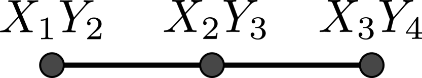
(a) $\mathfrak{a}_{1}(4)$

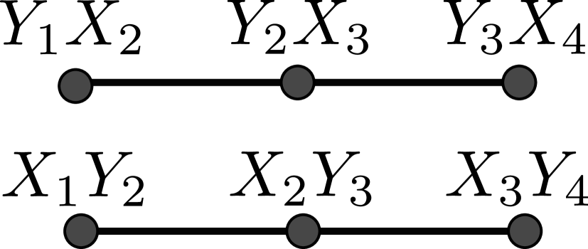
(b) $\mathfrak{a}_{2}(4)$

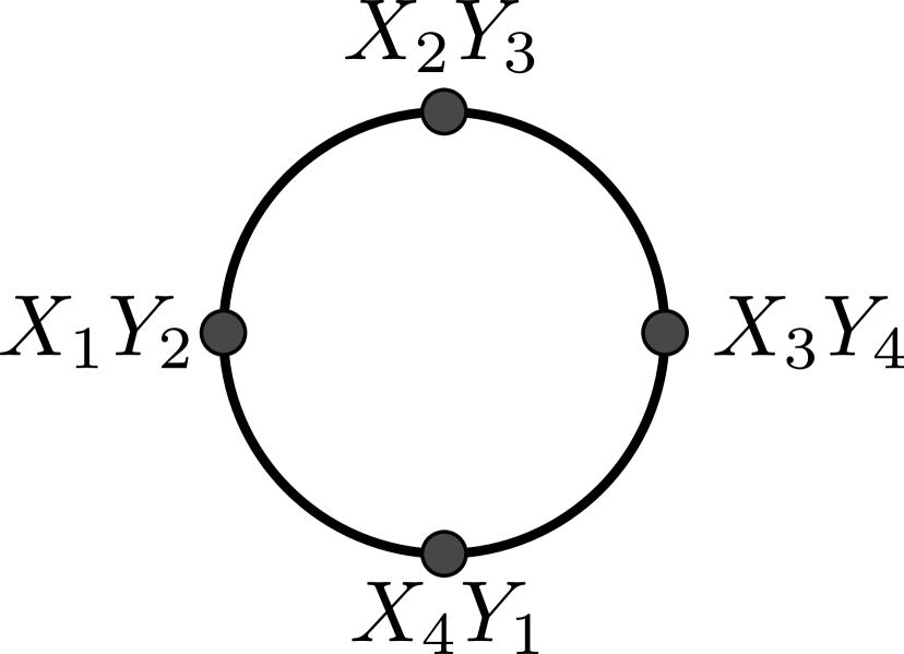
(c) $\mathfrak{a}_{2}^{\circ}(4)$

Figure S1: Frustration graphs for several examples in our classification for $n=4$. (a) A frustration graph given by a line. (b) A frustration graph consisting of two disjoint lines. (c) A circular frustration graph.

In this subsection, we review the notion of frustration graph, which is a useful visualization tool; see e.g. [110, 111, 100]. We determine the DLA in the cases when the frustration graph is a line or a circle, and apply these results to identify several of our Lie algebras, namely, $\mathfrak{a}_{k}(n)$ and $\mathfrak{a}_{k}^{\circ}(n)$ for $k=1,2,4,8,14$.

Definition C.1.

Given a set of Pauli strings $\mathcal{A}\subset\mathcal{P}_{n}$, its frustration graph is the graph with a set of vertices $\mathcal{A}$ and edges connecting all pairs of vertices $a,b\in\mathcal{A}$ such that $[a,b]\neq 0$.

The frustration graph makes it especially easy to determine when two subsets of the generating set $\mathcal{A}$ commute with each other: it means that they are disconnected from each other in the frustration graph. Suppose that $\mathcal{A}=\mathcal{A}_{1}\sqcup\mathcal{A}_{2}$ is a disjoint union of subsets with disconnected frustration graphs. Then

$$\langle\mathcal{A}_{1}\sqcup\mathcal{A}_{2}\rangle_{\mathrm{Lie}}=\langle\mathcal{A}_{1}\rangle_{\mathrm{Lie}}\oplus\langle\mathcal{A}_{2}\rangle_{\mathrm{Lie}}$$ (C14)

is a direct sum of commuting subalgebras. This is illustrated in Figure S1.

In the next proposition, we determine the DLA of a line frustration graph.

Proposition C.1.

Suppose that the frustration graph of $\mathcal{A}=\{a_{1},\dots,a_{N}\}\subset\mathcal{P}_{n}$ is a line, so that $[a_{j},a_{k}]\neq 0$ for $1\leq j<k\leq N$ if and only if $k=j+1$. Then

$$\langle\mathcal{A}\rangle_{\mathrm{Lie}}\cong\mathfrak{so}(N+1),$$

and a basis for it is given by $\{i^{k-j}L_{j,k}\}_{1\leq j<k\leq N+1}$, where $i$ is the imaginary unit and

$$L_{j,k}:=a_{j}\cdot a_{j+1}\cdots a_{k-1}\qquad(1\leq j<k\leq N+1)$$ (C15)

are products over line segments.

Proof.

Recall that $\langle\mathcal{A}\rangle_{\mathrm{Lie}}$ is the subalgebra of $\mathfrak{su}(2^{n})$ generated by the subset $i\mathcal{A}\subset\mathfrak{su}(2^{n})$ (see Definition A.1). First, let us us prove that all $i^{k-j}L_{j,k}$ are in $\langle\mathcal{A}\rangle_{\mathrm{Lie}}$. For $k=j+1$, we have $iL_{j,j+1}:=ia_{j}\in i\mathcal{A}\subseteq\langle\mathcal{A}\rangle_{\mathrm{Lie}}$. Suppose, by induction on $k-j$, that $i^{k-j}L_{j,k}\in\langle\mathcal{A}\rangle_{\mathrm{Lie}}$ for some $1<j<k\leq N+1$; then we will show that $i^{k-j+1}L_{j-1,k}\in\langle\mathcal{A}\rangle_{\mathrm{Lie}}$. By definition,

$$L_{j-1,k}=a_{j-1}\cdot a_{j}\cdot a_{j+1}\cdots a_{k-1}=a_{j-1}\cdot L_{j,k},$$

and by assumption, $a_{j-1}$ anticommutes with $a_{j}$ and commutes with $a_{j+1},\dots,a_{k-1}$. Hence, $a_{j-1}$ anticommutes with $L_{j,k}$, which implies that

$$2i^{k-j+1}L_{j-1,k}=2i^{k-j+1}a_{j-1}\cdot L_{j,k}=i^{k-j+1}[a_{j-1},L_{j,k}]=[ia_{j-1},i^{k-j}L_{j,k}]\in\langle\mathcal{A}\rangle_{\mathrm{Lie}}.$$

This proves the claim that $i^{k-j}L_{j,k}\in\langle\mathcal{A}\rangle_{\mathrm{Lie}}$ for all $1\leq j<k\leq N+1$.

Similarly to above, one can check that ($1\leq j<k<l\leq N+1$):

$$[i^{k-j}L_{j,k},i^{l-k}L_{k,l}]=2i^{l-j}L_{j,l},\quad[i^{l-k}L_{k,l},i^{l-j}L_{j,l}]=2i^{k-j}L_{j,k},\quad[i^{l-j}L_{j,l},i^{k-j}L_{j,k}]=2i^{l-k}L_{k,l},$$ (C16)

and all other commutators (not following from skewsymmetry) are zero. In particular, the real linear span of all $i^{k-j}L_{j,k}$ is closed under the bracket, i.e., is a subalgebra of $\mathfrak{su}(2^{n})$. Since $\langle\mathcal{A}\rangle_{\mathrm{Lie}}$ is the minimal (under inclusion) subalgebra of $\mathfrak{su}(2^{n})$ containing $i\mathcal{A}$, it follows that

$$\langle\mathcal{A}\rangle_{\mathrm{Lie}}=\mathrm{span}\{i^{k-j}L_{j,k}\}_{1\leq j<k\leq N+1}.$$

Recall that $\mathfrak{so}(N+1)=\mathfrak{so}(N+1,\mathbb{R})$ is the Lie algebra of all skewsymmetric $(N+1)\times(N+1)$ real matrices; see (A7). Consider the standard basis $\{E_{j,k}\}_{1\leq j,k\leq N+1}$ of $\mathfrak{gl}(N+1,\mathbb{R})$, where $E_{j,k}$ is the matrix with $(j,k)$-entry $=1$ and all other entries $=0$. Then a basis for $\mathfrak{so}(N+1)$ is $\{F_{j,k}:=E_{j,k}-E_{k,j}\}_{1\leq j<k\leq N+1}$. Using that

$$[E_{j,k},E_{l,m}]=\delta_{k,l}E_{j,m}-\delta_{j,m}E_{l,k},$$

it is easy to see that

$$[F_{j,k},F_{k,l}]=F_{j,l},\quad[F_{k,l},F_{j,l}]=F_{j,k},\quad[F_{j,l},F_{j,k}]=F_{k,l},\quad\text{for}\quad 1\leq j<k<l\leq N+1.$$

Hence, the matrices $2F_{j,k}$ satisfy the same commutation relations as $i^{k-j}L_{j,k}$ given in (C16). This means that the map $\mathfrak{so}(N+1)\to\langle\mathcal{A}\rangle_{\mathrm{Lie}}$ that sends $2F_{j,k}$ to $i^{k-j}L_{j,k}$ is a Lie algebra homomorphism. Its kernel is an ideal in $\mathfrak{so}(N+1)$, but since $\mathfrak{so}(N+1)$ is simple, it has no non-zero proper ideals. Therefore, this map is an isomorphism. ∎

Remark C.1.

One can see from the above proposition that, for linear frustration graphs, the dimension of the DLA scales quadratically with the number of generators. This was observed for free fermionic models in [112, 34, 35, 36, 37], where the number of generators is proportional to the system size and the circuit gate complexity is quadratic with respect to the system size. These models are fast forwardable along with the other Hamiltonians given in [110, 111, 100], and the fundamental reason for this is the polynomial scaling of the DLA.

After a Jordan–Wigner transformation, it can be shown that the algebra of free fermions on $n$ sites can be generated by $\{Z_{1},X_{1}X_{2},Z_{2},X_{2}X_{3},Z_{3},\dots,X_{n-1}X_{n},Z_{n}\}$, which will be shown to be equivalent to $\mathfrak{a}_{14}(n)$ in Lemma C.6. These generators have a linear frustration graph with $2n-1$ vertices; hence, its DLA is $\mathfrak{so}(2n)$.

Next, we consider the case when the frustration graph is a circle.

Proposition C.2.

Suppose that the frustration graph of $\mathcal{A}=\{a_{1},\dots,a_{N}\}\subset\mathcal{P}_{n}$ is a circle with $N\geq 3$, so that $[a_{j},a_{k}]\neq 0$ for $1\leq j<k\leq N$ if and only if $k=j+1$ or $j=1$, $k=N$. Then

$$\langle\mathcal{A}\rangle_{\mathrm{Lie}}\cong\mathfrak{so}(N)\oplus\mathfrak{so}(N),$$

and it has a basis $\{i^{k-j}L_{j,k},i^{N+k-j}C\cdot L_{j,k}\}_{1\leq j<k\leq N}$, where $i$ is the imaginary unit, $L_{j,k}$ are defined in (C15), and

$$C:=a_{1}\cdot a_{2}\cdots a_{N-1}\cdot a_{N}.$$ (C17)

Proof.

First, notice that $[C,a_{j}]=0$ for all $1\leq j\leq N$, because $a_{j}$ does not commute only with its two neighboring vertices in the circle frustration graph. Moreover, using that $a_{j}\cdot a_{j}=I^{\otimes n}$ (cf. Lemma A.1), we get $C\cdot C=(-1)^{N}I^{\otimes n}$. From here, we deduce that

$$[i^{N}C,i^{k-j}L_{j,k}]=0,\qquad(i^{N}C)\cdot(i^{N}C)=I^{\otimes n}.$$ (C18)

If we remove any vertex from the frustration graph of $\mathcal{A}$, we obtain a line frustration graph. By Proposition C.1, we know that

$$i^{k-j}L_{j,k}\in\langle a_{1},\dots,a_{N-1}\rangle_{\mathrm{Lie}}\subseteq\langle\mathcal{A}\rangle_{\mathrm{Lie}},\qquad 1\leq j<k\leq N,$$

and these elements form a basis for the subalgebra $\langle a_{1},\dots,a_{N-1}\rangle_{\mathrm{Lie}}\cong\mathfrak{so}(N)$. In particular, we have

$$\{ia_{1},\dots,ia_{N-1}\}\subset\langle a_{1},\dots,a_{N-1}\rangle_{\mathrm{Lie}}=\mathrm{span}_{\mathbb{R}}\{i^{k-j}L_{j,k}\}_{1\leq j<k\leq N}.$$

Similarly, the set $\mathcal{A}\setminus\{a_{k-1}\}=\{a_{k},a_{k+1},\dots,a_{N},a_{1},\dots,a_{k-2}\}$ has a line frustration graph and its subset $\{a_{k},a_{k+1},\dots,a_{N},a_{1},\dots,a_{j-1}\}$ is a line segment for $1\leq j<k\leq N$. Hence, again by Proposition C.1,

$$i^{N+k-j}C\cdot L_{j,k}=\pm i^{N-k+j}a_{k}\cdot a_{k+1}\cdots a_{N}\cdot a_{1}\cdots a_{j-1}\in\langle\mathcal{A}\setminus\{a_{k-1}\}\rangle_{\mathrm{Lie}}\subseteq\langle\mathcal{A}\rangle_{\mathrm{Lie}},\qquad 1\leq j<k\leq N.$$

In particular, the choice $j=1$, $k=N$ gives

$$i^{N+N-1}C\cdot L_{1,N}=\pm ia_{N}.$$

The above discussion implies that

$$i\mathcal{A}\subset\mathcal{L}:=\mathrm{span}_{\mathbb{R}}\{i^{k-j}L_{j,k},i^{N+k-j}C\cdot L_{j,k}\}_{1\leq j<k\leq N}\subseteq\langle\mathcal{A}\rangle_{\mathrm{Lie}}.$$

We claim that the vector space $\mathcal{L}$ is closed under the Lie bracket. Indeed, we already know that $\mathrm{span}_{\mathbb{R}}\{i^{k-j}L_{j,k}\}$ is closed. For the other brackets, we use that from (C18), we have:

$$[i^{k-j}L_{j,k},i^{N+m-l}C\cdot L_{l,m}] =i^{N}C\cdot[i^{k-j}L_{j,k},i^{m-l}L_{l,m}],$$

$$[i^{N+k-j}C\cdot L_{j,k},i^{N+m-l}C\cdot L_{l,m}] =[i^{k-j}L_{j,k},i^{m-l}L_{l,m}].$$

As the Lie algebra $\mathcal{L}$ contains $i\mathcal{A}$, it must contain $\langle\mathcal{A}\rangle_{\mathrm{Lie}}$. Therefore, $\mathcal{L}=\langle\mathcal{A}\rangle_{\mathrm{Lie}}$.

Using (C18) again (or from the above brackets), we see that

$$\langle\mathcal{A}\rangle_{\mathrm{Lie}}=\mathrm{span}_{\mathbb{R}}\{(I^{\otimes n}+i^{N}C)\cdot i^{k-j}L_{j,k}\}_{1\leq j<k\leq N}\oplus\mathrm{span}_{\mathbb{R}}\{(I^{\otimes n}-i^{N}C)\cdot i^{k-j}L_{j,k}\}_{1\leq j<k\leq N}$$

is isomorphic as a Lie algebra to a direct sum of two copies of $\mathrm{span}_{\mathbb{R}}\{i^{k-j}L_{j,k}\}_{1\leq j<k\leq N}\cong\mathfrak{so}(N)$. Therefore, $\langle\mathcal{A}\rangle_{\mathrm{Lie}}\cong\mathfrak{so}(N)\oplus\mathfrak{so}(N)$. ∎

Remark C.2.

A circular frustration graph corresponds to free fermionic evolution controlled with one ancilla, where the ancilla degree of freedom can be readily found as the operator $C$ defined in (C17). As expected, this is not the only example. Some periodic $1$-dimensional spin systems such as TFXY, XY and Kitaev models also have DLAs that are generated from Pauli strings with a circular frustration graph. For those spin models, $C=ZZ\cdots Z$.

Applying the results of Propositions C.1, C.2, in the following lemmas we determine the Lie algebras $\mathfrak{a}_{k}(n)$ and $\mathfrak{a}_{k}^{\circ}(n)$ for $k=1,2,4,8,14$. Examples are presented in Figures S2 and S3.

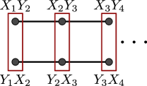
(a) $\mathfrak{a}_{2}(n)$

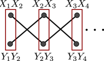
(b) $\mathfrak{a}_{4}(n)$

Figure S2: Frustration graphs for $\mathfrak{a}_{2}(n)$ and $\mathfrak{a}_{4}(n)$. The red boxes denote a generator acting on the site ($i$, $i+1$). Both frustrations graphs are given by two disjoint lines for any $n$; hence we can conclude that $\mathfrak{a}_{2}(n)\cong\mathfrak{a}_{4}(n)$ (cf. Lemma C.3).

Lemma C.6.

We have:

$$\begin{split}\mathfrak{a}_{1}(n)&\cong\mathfrak{so}(n),\\ \mathfrak{a}_{2}(n)&\cong\mathfrak{a}_{4}(n)\cong\mathfrak{so}(n)\oplus\mathfrak{so}(n),\\ \mathfrak{a}_{8}(n)&\cong\mathfrak{so}(2n-1),\\ \mathfrak{a}_{14}(n)&\cong\mathfrak{so}(2n).\end{split}$$

Proof.

The proof is based on the frustration graphs of the generating sets of these Lie algebras (see Sect. I, IV).

Generators of $\mathfrak{a}_{1}(n)$ are $XY$ on each adjacent pair of qubits:

$$X_{1}Y_{2},X_{2}Y_{3},X_{3}Y_{4},\dots,X_{n-1}Y_{n}.$$

These form a linear frustration graph with $n-1$ vertices, leading to $\mathfrak{a}_{1}(n)\cong\mathfrak{so}(n)$ (see Figure S3(a)).

The Lie algebra $\mathfrak{a}_{2}(n)$ is generated by $XY$ and $YX$ on adjacent pairs of qubits:

$$X_{1}Y_{2},X_{2}Y_{3},X_{3}Y_{4},\dots,X_{n-1}Y_{n}\qquad\text{and}\qquad Y_{1}X_{2},Y_{2}X_{3},Y_{3}X_{4},\dots,Y_{n-1}X_{n}.$$

Both of these form linear frustration graphs with $n-1$ vertices, and commute with each other (see Figure S2). Thus, $\mathfrak{a}_{2}(n)\cong\mathfrak{so}(n)\oplus\mathfrak{so}(n)$. Note that $\mathfrak{a}_{4}(n)\cong\mathfrak{a}_{2}(n)$ due to Lemma C.3 (see also Figure S2).

Since $\mathfrak{a}_{8}=\mathrm{span}\{XX,XZ,IY\}=\langle XX,IY\rangle_{\mathrm{Lie}}$, we can generate $\mathfrak{a}_{8}(n)$ by:

$$X_{1}X_{2},Y_{2},X_{2}X_{3},Y_{3},X_{3}X_{4},Y_{4},\dots,X_{n-1}X_{n},Y_{n}.$$ (C19)

These form a linear frustration graph with $2(n-1)$ vertices; hence $\mathfrak{a}_{8}(n)\cong\mathfrak{so}(2n-1)$ (see Figure S3(b)).

Similarly, note that

$$\mathfrak{a}_{14}=\mathrm{span}\{XX,YY,XY,YX,ZI,IZ\}=\langle XX,ZI,IZ\rangle_{\mathrm{Lie}},$$

because $[XX,ZI]=2iYX$, $[XX,IZ]=2iXY$, and $[XY,ZI]=-2iYY$. Thus, $\mathfrak{a}_{14}(n)$ is generated by:

$$Z_{1},X_{1}X_{2},Z_{2},X_{2}X_{3},Z_{3},X_{3}X_{4},Z_{4},\dots,X_{n-1}X_{n},Z_{n},$$ (C20)

which gives a linear frustration graph with $2n-1$ vertices. Hence $\mathfrak{a}_{14}(n)\cong\mathfrak{so}(2n)$ (see Figure S3(c)). ∎

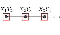
(a) $\mathfrak{a}_{1}(n)$

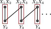
(b) $\mathfrak{a}_{8}(n)$

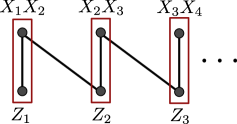
(c) $\mathfrak{a}_{14}(n)$

Figure S3: Visualization of the frustration graphs of generators of certain Lie algebras. The red boxes denote a generator acting on the site ($i$, $i+1$). For the three cases $\mathfrak{a}_{1}(n)$, $\mathfrak{a}_{8}(n)$ and $\mathfrak{a}_{14}(n)$, we see that the frustration graph is a line for any $n$. For (a), the 2-site DLA $\mathfrak{a}_{1}(2)\cong\mathfrak{u}(1)$, but as $n$ grows we find $\mathfrak{a}_{1}(n)\cong\mathfrak{so}(n)$. (b) The frustration graph is a line with $2n-2$ vertices; hence $\mathfrak{a}_{8}(n)\cong\mathfrak{so}(2n-1)$. (c) The frustration graph is a line with $2n-1$ vertices, giving $\mathfrak{a}_{14}(n)\cong\mathfrak{so}(2n)$.

Lemma C.7.

We have $\mathfrak{a}_{k}^{\circ}(n)\cong\mathfrak{a}_{k}(n)^{\oplus 2}$ for $k=1,2,14$ and $n\geq 3$.

Proof.

The Lie algebra $\mathfrak{a}_{1}^{\circ}(n)$ is generated by $XY$ applied on adjacent qubits, including periodic boundary conditions:

$$X_{1}Y_{2},X_{2}Y_{3},X_{3}Y_{4},\dots,X_{n-1}Y_{n},X_{n}Y_{1}.$$

The frustration graph is a circle with $n$ vertices. Therefore, $\mathfrak{a}_{1}^{\circ}(n)\cong\mathfrak{so}(n)^{\oplus 2}\cong\mathfrak{a}_{1}(n)^{\oplus 2}$.

The Lie algebra $\mathfrak{a}_{2}^{\circ}(n)$ is generated by $XY$ and $YX$ applied on adjacent qubits with periodic boundary conditions:

$$X_{1}Y_{2},X_{2}Y_{3},X_{3}Y_{4},\dots,X_{n-1}Y_{n},X_{n}Y_{1}\qquad\text{and}\qquad Y_{1}X_{2},Y_{2}X_{3},Y_{3}X_{4},\dots,Y_{n-1}X_{n},Y_{n}X_{1}.$$

These form two circular frustration graphs with $n$ vertices that are disconnected from each other. Thus, $\mathfrak{a}_{2}^{\circ}(n)\cong\mathfrak{so}(n)^{\oplus 2}\oplus\mathfrak{so}(n)^{\oplus 2}\cong\mathfrak{a}_{2}(n)^{\oplus 2}$.

Using the generating set (C20) of $\mathfrak{a}_{14}(n)$, we see that $\mathfrak{a}_{14}^{\circ}(n)$ can be generated by:

$$Z_{1},X_{1}X_{2},Z_{2},X_{2}X_{3},Z_{3},X_{3}X_{4},Z_{4},\dots,X_{n-1}X_{n},Z_{n},X_{n}X_{1}.$$

This leads to a circular frustration graph with $2n$ vertices, so $\mathfrak{a}_{14}^{\circ}(n)\cong\mathfrak{so}(2n)^{\oplus 2}\cong\mathfrak{a}_{14}(n)^{\oplus 2}$. ∎

Lemma C.8.

We have $\mathfrak{a}_{8}^{\circ}(n)\cong\mathfrak{a}_{14}^{\circ}(n)\cong\mathfrak{so}(2n)^{\oplus 2}$ for all $n\geq 3$.

Proof.

The generating sets (C19) and (C20) of $\mathfrak{a}_{8}(n)$ and $\mathfrak{a}_{14}(n)$ are the same after swapping $Y\rightleftharpoons Z$, except that $\mathfrak{a}_{8}(n)$ does not have $Y_{1}$. When the periodic boundary condition is applied, this difference disappears and we obtain that $\mathfrak{a}_{8}^{\circ}(n)\cong\mathfrak{a}_{14}^{\circ}(n)$. ∎

Lemma C.9.

We have $\mathfrak{a}_{4}^{\circ}(n)\cong\begin{cases}\mathfrak{so}(2n)^{\oplus 2},&n\;\mathrm{odd},\\ \mathfrak{so}(n)^{\oplus 4},&n\;\mathrm{even}.\end{cases}$

Proof.

As $\mathfrak{a}_{4}=\langle XX,YY\rangle_{\mathrm{Lie}}$, the generators of $\mathfrak{a}_{4}^{\circ}(n)$ are:

$$X_{1}X_{2},Y_{1}Y_{2},X_{2}X_{3},Y_{2}Y_{3},\dots,X_{n-1}X_{n},Y_{n-1}Y_{n},X_{n}X_{1},Y_{n}Y_{1}.$$

For odd $n$, these generators form a circular frustration graph with $2n$ vertices:

$$X_{1}X_{2},Y_{2}Y_{3},X_{3}X_{4},Y_{4}Y_{5},\dots,Y_{n-1}Y_{n},X_{n}X_{1},Y_{1}Y_{2},X_{2}X_{3},Y_{3}Y_{4},X_{4}X_{5},\dots,X_{n-1}X_{n},Y_{n}Y_{1}.$$

Hence, in this case, $\mathfrak{a}_{4}^{\circ}(n)\cong\mathfrak{so}(2n)^{\oplus 2}$.

When $n$ is even, the generators form two disjoint circles with $n$ vertices each:

$$X_{1}X_{2},Y_{2}Y_{3},X_{3}X_{4},\dots,X_{n-1}X_{n},Y_{n}Y_{1}\qquad\text{and}\qquad Y_{1}Y_{2},X_{2}X_{3},Y_{3}Y_{4},\dots,Y_{n-1}Y_{n},X_{n}X_{1}.$$

In this case, we get $\mathfrak{a}_{4}^{\circ}(n)\cong\mathfrak{so}(n)^{\oplus 2}\oplus\mathfrak{so}(n)^{\oplus 2}$. ∎

Remark C.3.

Notice that, although $\mathfrak{a}_{2}(n)\cong\mathfrak{a}_{4}(n)$ for all $n\geq 3$, we have $\mathfrak{a}_{2}^{\circ}(n)\not\cong\mathfrak{a}_{4}^{\circ}(n)$ for odd $n$.

IV Stabilizers, commutants, and centralizers

For any Pauli string $A\in\mathcal{P}_{k}$, we will use the notation $P_{A}=AAA\cdots\in\mathcal{P}_{n}$ truncated to the $n$-th qubit. For example,

$$P_{X} =XXX\cdots, P_{YZ} =YZYZ\cdots, P_{ZY} =ZYZY\cdots,$$

$$P_{XYZ} =XYZXYZ\cdots, P_{YZX} =YZXYZX\cdots, P_{ZXY} =ZXYZXY\cdots,$$

where these are viewed as elements of $\mathcal{P}_{n}$. In particular, $P_{I}=I\cdots I=I^{\otimes n}$. Recall that $\pm\mathcal{P}_{n}\cup\pm i\mathcal{P}_{n}$ is a group under the matrix product, the Pauli group (see Sect. I).

For any set of matrices $\mathcal{A}\subseteq\mathbb{C}^{2^{n}\times 2^{n}}$, we define its stabilizer $\mathrm{St}(\mathcal{A})\subseteq\mathcal{P}_{n}$ as the set of all Pauli strings that commute with every element of $\mathcal{A}$. It is clear that $\mathrm{St}(\mathcal{A})$ is closed under multiplication, so after allowing appropriate powers of $i$ it is a group. There are two related, and essentially equivalent, notions called the commutant and centralizer. All of these consist of elements commuting with the given set $\mathcal{A}$ but differ in where such elements are and what structure they form: the stabilizer is a subgroup of the Pauli group (up to factors of $\pm 1,\pm i$); the commutant is a subalgebra of the associative algebra $\mathbb{C}^{2^{n}\times 2^{n}}$ of all complex matrices; while the centralizer is a subalgebra of the real Lie algebra $\mathfrak{su}(2^{n})$. The precise relations are explained in the following two remarks.

Remark C.4.

The commutant of a set $\mathcal{A}\subseteq\mathbb{C}^{2^{n}\times 2^{n}}$ is defined as the set $\mathcal{A}^{\prime}$ of all $2^{n}\times 2^{n}$ complex matrices that commute with all elements of $\mathcal{A}$. Then $\mathcal{A}^{\prime}$ is closed under addition, multiplication, and multiplication by any complex scalar, i.e., it is an associative algebra over $\mathbb{C}$. It is easy to see that $\mathcal{A}^{\prime}=\mathrm{span}_{\mathbb{C}}\mathrm{St}(\mathcal{A})$ is the complex linear span of the stabilizer $\mathrm{St}(\mathcal{A})$.

Note that $\mathcal{A}\subseteq\mathcal{A}^{\prime\prime}:=(\mathcal{A}^{\prime})^{\prime}$. By (a finite-dimensional version of) von Neumann’s Double Commutant Theorem (see e.g. [44], Theorem 6.2.5), $\mathcal{A}^{\prime\prime}$ is the associative algebra generated by $\mathcal{A}$. In particular, for a complex vector space $\mathcal{A}$, we have $\mathcal{A}^{\prime\prime}=\mathcal{A}+\mathbb{C}I^{\otimes n}$ if and only if $\mathcal{A}$ is closed under multiplication.

Remark C.5.

The centralizer of a set $\mathcal{A}\subseteq\mathfrak{su}(2^{n})$ is the set $\mathfrak{su}(2^{n})^{\mathcal{A}}\subseteq\mathfrak{su}(2^{n})$ of all traceless skew-Hermitian $2^{n}\times 2^{n}$ matrices that commute with all elements of $\mathcal{A}$. Then $\mathfrak{su}(2^{n})^{\mathcal{A}}$ is closed under addition, commutator, and multiplication by any real scalar, i.e., it is a Lie subalgebra of $\mathfrak{su}(2^{n})$. It is easy to see that $\mathfrak{su}(2^{n})^{\mathcal{A}}=\mathrm{span}(\mathrm{St}(\mathcal{A})\setminus\{I^{\otimes n}\})$ is the real span of $i(\mathrm{St}(\mathcal{A})\setminus\{I^{\otimes n}\})$.

When $\mathfrak{s}\subseteq\mathfrak{su}(2^{n})$ is a Lie subalgebra, a given Pauli string commutes with all elements of $\mathfrak{s}$ if and only if it commutes with all generators of $\mathfrak{s}$. In other words, we have

$$\mathrm{St}(\langle\mathcal{A}\rangle_{\mathrm{Lie}})=\mathrm{St}(\mathcal{A}).$$ (C21)

Thus, to determine the stabilizers of our Lie subalgebras of $\mathfrak{su}(2^{n})$, it suffices to find the stabilizers of their generating sets. In the case $n=2$, it is easy to find the answer by inspection, which is given as follows:

$$\mathrm{St}(\mathfrak{a}_{0}) =\{II,IX,XI,XX,YY,YZ,ZY,ZZ\},$$

$$\mathrm{St}(\mathfrak{a}_{1}) =\{II,IY,XI,XY,YX,YZ,ZX,ZZ\},$$

$$\mathrm{St}(\mathfrak{a}_{2}) =\{II,XY,YX,ZZ\},$$

$$\mathrm{St}(\mathfrak{a}_{3}) =\mathrm{St}(\mathfrak{a}_{6})=\{II,XX,YZ,ZY\},$$

$$\mathrm{St}(\mathfrak{a}_{4}) =\mathrm{St}(\mathfrak{a}_{7})=\{II,XX,YY,ZZ\},$$

$$\mathrm{St}(\mathfrak{a}_{5}) =\mathrm{St}(\mathfrak{a}_{10})=\{II,XY,YZ,ZX\},$$

$$\mathrm{St}(\mathfrak{a}_{8}) =\{II,XI,YY,ZY\},$$

$$\mathrm{St}(\mathfrak{a}_{9}) =\{II,XI,YX,ZX\},$$

$$\mathrm{St}(\mathfrak{a}_{11}) =\{II,XY\},$$

$$\mathrm{St}(\mathfrak{a}_{12}) =\mathrm{St}(\mathfrak{a}_{17})=\mathrm{St}(\mathfrak{a}_{19})=\{II,YZ\},$$

$$\mathrm{St}(\mathfrak{a}_{13}) =\mathrm{St}(\mathfrak{a}_{20})=\{II,XX\},$$

$$\mathrm{St}(\mathfrak{a}_{14}) =\{II,ZZ\},$$

$$\mathrm{St}(\mathfrak{a}_{15}) =\mathrm{St}(\mathfrak{b}_{2})=\mathrm{St}(\mathfrak{b}_{4})=\{II,XI\},$$

$$\mathrm{St}(\mathfrak{b}_{0}) =\mathrm{St}(\mathfrak{b}_{1})=\{II,XX,XI,IX\},$$

$$\mathrm{St}(\mathfrak{a}_{k}) =\mathrm{St}(\mathfrak{b}_{3})=\{II\},\qquad k=16,18,21,22.$$

Using that, we can find the stabilizers of the subalgebras of $\mathfrak{su}(2^{n})$.

Proposition C.3.

For $n\geq 3$, we have the following stabilizers:

$$\mathrm{St}(\mathfrak{a}_{0}(n)) =\{I,X\}^{\otimes n}\cup\{Y,Z\}^{\otimes n},$$

$$\mathrm{St}(\mathfrak{a}_{2}(n)) =\{P_{I},P_{XY},P_{YX},P_{Z}\},$$

$$\mathrm{St}(\mathfrak{a}_{3}(n)) =\mathrm{St}(\mathfrak{a}_{6}(n))=\{P_{I},P_{X},P_{YZ},P_{ZY}\},$$

$$\mathrm{St}(\mathfrak{a}_{4}(n)) =\mathrm{St}(\mathfrak{a}_{7}(n))=\{P_{I},P_{X},P_{Y},P_{Z}\},$$

$$\mathrm{St}(\mathfrak{a}_{5}(n)) =\mathrm{St}(\mathfrak{a}_{10}(n))=\{P_{I},P_{XYZ},P_{YZX},P_{ZXY}\},$$

$$\mathrm{St}(\mathfrak{a}_{8}(n)) =\{P_{I},P_{Y},X_{1},ZY\cdots Y\},$$

$$\mathrm{St}(\mathfrak{a}_{9}(n)) =\{P_{I},X_{1},Y_{1}X_{2},Z_{1}X_{2}\},$$

$$\mathrm{St}(\mathfrak{a}_{13}(n)) =\mathrm{St}(\mathfrak{a}_{20}(n))=\{P_{I},P_{X}\},$$

$$\mathrm{St}(\mathfrak{a}_{14}(n)) =\{P_{I},P_{Z}\},$$

$$\mathrm{St}(\mathfrak{a}_{15}(n)) =\mathrm{St}(\mathfrak{b}_{2}(n))=\mathrm{St}(\mathfrak{b}_{4}(n))=\{P_{I},X_{1}\},$$

$$\mathrm{St}(\mathfrak{b}_{0}(n)) =\mathrm{St}(\mathfrak{b}_{1}(n))=\{I,X\}^{\otimes n},$$

$$\mathrm{St}(\mathfrak{a}_{k}(n)) =\mathrm{St}(\mathfrak{b}_{3}(n))=\{P_{I}\},\qquad k=11,12,16{-}19,21,22.$$

Proof.

Recall that, for any subalgebra $\mathfrak{a}\subseteq\mathfrak{su}(4)$, the subalgebra $\mathfrak{a}(n)\subseteq\mathfrak{su}(2^{n})$ is generated by all Pauli strings $A_{i}B_{i+1}$, where $AB\in\mathfrak{a}$, $1\leq i\leq n-1$ (see (B6)). Thus, a Pauli string $P^{1}\otimes\cdots\otimes P^{n}\in\mathcal{P}_{n}$ is in $\mathrm{St}(\mathfrak{a}(n))$ if and only if $P^{i}\otimes P^{i+1}\in\mathrm{St}(\mathfrak{a})$ for all $1\leq i\leq n-1$. Using this observation and the knowledge of all $\mathrm{St}(\mathfrak{a})$, it is straightforward to determine $\mathrm{St}(\mathfrak{a}(n))$.

Let us consider the case of $\mathfrak{a}_{2}$ as an illustration. Since $\mathrm{St}(\mathfrak{a}_{2})=\{II,XY,YX,ZZ\}$, we want to find all Pauli strings, such that for any two consecutive qubits, we have either $II$, $XY$, $YX$, or $ZZ$. The only possible such strings are $I\cdots I$, $XYXY\cdots$, $YXYX\cdots$, or $Z\cdots Z$. ∎

The answer for $\mathrm{St}(\mathfrak{a}_{1}(n))$ is given without proof in Remark C.6 below, as it is more complicated but not needed for the rest of the paper. For future use, we will need the centers of some of the above stabilizers. Let us recall that the center $Z(G)$ of a group $G$ consists of all $z\in G$ that commute with every $g\in G$. In particular, a group $G$ is Abelian if and only if $Z(G)=G$.

Lemma C.10.

For $n\geq 3$, we have the following centers:

$$Z\bigl{(}\mathrm{St}(\mathfrak{a}_{2}(n))\bigr{)} =\begin{cases}\{P_{I},P_{XY},P_{YX},P_{Z}\},&n\;\;\mathrm{even},\\ \{P_{I}\},&n\;\;\mathrm{odd},\end{cases}$$

$$Z\bigl{(}\mathrm{St}(\mathfrak{a}_{3}(n))\bigr{)} =Z\bigl{(}\mathrm{St}(\mathfrak{a}_{6}(n))\bigr{)}=\begin{cases}\{P_{I},P_{X},P_{YZ},P_{ZY}\},&n\;\;\mathrm{even},\\ \{P_{I}\},&n\;\;\mathrm{odd},\end{cases}$$

$$Z\bigl{(}\mathrm{St}(\mathfrak{a}_{4}(n))\bigr{)} =Z\bigl{(}\mathrm{St}(\mathfrak{a}_{7}(n))\bigr{)}=\begin{cases}\{P_{I},P_{X},P_{Y},P_{Z}\},&n\;\;\mathrm{even},\\ \{P_{I}\},&n\;\;\mathrm{odd},\end{cases}$$

$$Z\bigl{(}\mathrm{St}(\mathfrak{a}_{5}(n))\bigr{)} =Z\bigl{(}\mathrm{St}(\mathfrak{a}_{10}(n))\bigr{)}=\begin{cases}\{P_{I},P_{XYZ},P_{YZX},P_{ZXY}\},&n\;\;\mathrm{even},\\ \{P_{I}\},&n\;\;\mathrm{odd},\end{cases}$$

$$Z\bigl{(}\mathrm{St}(\mathfrak{a}_{13}(n))\bigr{)} =Z\bigl{(}\mathrm{St}(\mathfrak{a}_{20}(n))\bigr{)}=\{P_{I},P_{X}\},$$

$$Z\bigl{(}\mathrm{St}(\mathfrak{a}_{14}(n))\bigr{)} =\{P_{I},P_{Z}\},$$

$$Z\bigl{(}\mathrm{St}(\mathfrak{a}_{15}(n))\bigr{)} =\{P_{I},X_{1}\},$$

$$Z\bigl{(}\mathrm{St}(\mathfrak{a}_{k}(n))\bigr{)} =\{P_{I}\},\qquad k=0,8,9,11,12,16{-}19,21,22.$$

Next, we determine the stabilizers in the periodic case.

Proposition C.4.

For $n\geq 3$, we have the following stabilizers:

$$\mathrm{St}(\mathfrak{a}_{0}^{\circ}(n)) =\{I,X\}^{\otimes n}\cup\{Y,Z\}^{\otimes n},$$

$$\mathrm{St}(\mathfrak{a}_{2}^{\circ}(n)) =\begin{cases}\{P_{I},P_{XY},P_{YX},P_{Z}\},&n\;\;\mathrm{even},\\ \{P_{I},P_{Z}\},&n\;\;\mathrm{odd},\end{cases}$$

$$\mathrm{St}(\mathfrak{a}_{3}^{\circ}(n)) =\mathrm{St}(\mathfrak{a}_{6}^{\circ}(n))=\begin{cases}\{P_{I},P_{X},P_{YZ},P_{ZY}\},&n\;\;\mathrm{even},\\ \{P_{I},P_{X}\},&n\;\;\mathrm{odd},\end{cases}$$

$$\mathrm{St}(\mathfrak{a}_{4}^{\circ}(n)) =\mathrm{St}(\mathfrak{a}_{7}^{\circ}(n))=\{P_{I},P_{X},P_{Y},P_{Z}\},$$

$$\mathrm{St}(\mathfrak{a}_{5}^{\circ}(n)) =\mathrm{St}(\mathfrak{a}_{10}^{\circ}(n))=\begin{cases}\{P_{I},P_{XYZ},P_{YZX},P_{ZXY}\},&n\equiv 0\mod 3,\\ \{P_{I}\},&n\equiv\pm 1\mod 3,\end{cases}$$

$$\mathrm{St}(\mathfrak{a}_{8}^{\circ}(n)) =\{P_{I},P_{Y}\},$$

$$\mathrm{St}(\mathfrak{a}_{13}^{\circ}(n)) =\mathrm{St}(\mathfrak{a}_{20}^{\circ}(n))=\{P_{I},P_{X}\},$$

$$\mathrm{St}(\mathfrak{a}_{14}^{\circ}(n)) =\{P_{I},P_{Z}\},$$

$$\mathrm{St}(\mathfrak{b}_{0}^{\circ}(n)) =\mathrm{St}(\mathfrak{b}_{1}^{\circ}(n))=\{I,X\}^{\otimes n},$$

$$\mathrm{St}(\mathfrak{a}_{k}^{\circ}(n)) =\mathrm{St}(\mathfrak{b}_{l}^{\circ}(n))=\{P_{I}\},\qquad k=9,11,12,15{-}19,21,22,\quad l=2,3,4.$$

Proof.

For any subalgebra $\mathfrak{a}\subseteq\mathfrak{su}(4)$, comparing the definitions of $\mathfrak{a}(n)$ and $\mathfrak{a}^{\circ}(n)$ (see (B5), (B6)), we see that $\mathrm{St}(\mathfrak{a}^{\circ}(n))$ consists of all Pauli strings $P^{1}\otimes\cdots\otimes P^{n}\in\mathrm{St}(\mathfrak{a}(n))$ such that $P^{n}\otimes P^{1}\in\mathrm{St}(\mathfrak{a})$. Thus, we determine $\mathrm{St}(\mathfrak{a}^{\circ}(n))$ by inspecting all elements of $\mathrm{St}(\mathfrak{a}(n))$. ∎

Remark C.6.

One can show that $\mathrm{St}(\mathfrak{a}_{1}(n))=\mathrm{St}(\mathfrak{a}_{1}^{\circ}(n))$, and as a group it is generated by the elements $P_{Z}$, $Y_{1}X_{2}$, $Y_{2}X_{3}$, $\dots$, $Y_{n-1}X_{n}$. This means that $\mathrm{St}(\mathfrak{a}_{1}(n))$ consists of all possible matrix products of these generators. For the center, we have $Z\bigl{(}\mathrm{St}(\mathfrak{a}_{1}(n))\bigr{)}=\{P_{I},P_{Z}\}$.

We also find the stabilizers in the permutation-invariant case.

Proposition C.5.

For $n\geq 3$, we have the following stabilizers:

$$\mathrm{St}(\mathfrak{a}_{0}^{\pi}(n)) =\{I,X\}^{\otimes n}\cup\{Y,Z\}^{\otimes n},$$

$$\mathrm{St}(\mathfrak{a}_{2}^{\pi}(n)) =\mathrm{St}(\mathfrak{a}_{14}^{\pi}(n))=\{P_{I},P_{Z}\},$$

$$\mathrm{St}(\mathfrak{a}_{4}^{\pi}(n)) =\mathrm{St}(\mathfrak{a}_{7}^{\pi}(n))=\{P_{I},P_{X},P_{Y},P_{Z}\},$$

$$\mathrm{St}(\mathfrak{a}_{6}^{\pi}(n)) =\mathrm{St}(\mathfrak{a}_{20}^{\pi}(n))=\{P_{I},P_{X}\},$$

$$\mathrm{St}(\mathfrak{b}_{0}^{\pi}(n)) =\mathrm{St}(\mathfrak{b}_{1}^{\pi}(n))=\{I,X\}^{\otimes n},$$

$$\mathrm{St}(\mathfrak{a}_{16}^{\pi}(n)) =\mathrm{St}(\mathfrak{b}_{3}^{\pi}(n))=\{P_{I}\}.$$

Proof.

For any subalgebra $\mathfrak{a}\subseteq\mathfrak{su}(4)$, from the definition of $\mathfrak{a}^{\pi}(n)$ (see (B9)), we see that $\mathrm{St}(\mathfrak{a}^{\pi}(n))$ consists of all Pauli strings $P^{1}\otimes\cdots\otimes P^{n}\in\mathcal{P}_{n}$ such that $P^{i}\otimes P^{j}\in\mathrm{St}(\mathfrak{a})$ for all $i\neq j$. Moreover, as we explained in Sect. IV, $\mathfrak{a}$ can be assumed itself invariant under the flip of the two qubits; so we only need to consider $\mathfrak{a}_{k}^{\pi}(n)$ for $k=0,2,4,6,7,14,16,20$ and $\mathfrak{b}_{l}^{\pi}(n)$ for $l=0,1,3$. ∎

We finish this subsection with an important lemma.

Lemma C.11.

The Lie algebras $\mathfrak{a}_{k}(n)$ have trivial centers for $1\leq k\leq 22$ and $n\geq 3$.

Proof.

Due to Lemma A.2, $\mathfrak{a}_{k}(n)$ has a basis $\mathcal{B}\subseteq i\mathcal{P}_{n}\cap\mathfrak{a}_{k}(n)$ consisting of Pauli strings. Suppose that $\mathfrak{a}_{k}(n)$ has a central element $c\neq 0$, and write $c$ as a linear combination of basis vectors:

$$c=\sum\alpha_{j}c_{j},\qquad\alpha_{j}\in\mathbb{R},\;\;\alpha_{j}\neq 0,\;\;c_{j}\in\mathcal{B}.$$

We claim that all $c_{j}$ in this expression are central too.

Indeed, suppose that $[b,c_{j}]\neq 0$ for some index $j$ and a basis vector $b\in\mathcal{B}$. Since $b,c_{j}\in i\mathcal{P}_{n}$, we have $[b,[b,c_{j}]]=-4c_{j}$ whenever $[b,c_{j}]\neq 0$, by Corollary A.1. Hence,

$$0=[b,[b,c]]=\sum\alpha_{j}[b,[b,c_{j}]]=-4\sum\nolimits^{\prime}\alpha_{j}c_{j},$$

where $\sum^{\prime}$ denotes the sum over all indices $j$ such that $[b,c_{j}]\neq 0$. This contradicts the fact that all $\alpha_{j}\neq 0$ and the vectors $c_{j}$ are linearly independent.

Therefore, without loss of generality, we can take $c\in\mathcal{B}$ to be itself one of the basis vectors. One can verify by inspection that the generators of $\mathfrak{a}_{k}(n)$ are not central for $1\leq k\leq 22$ and $n\geq 3$; for example, by checking that $Z\bigl{(}\mathrm{St}(\mathfrak{a}_{k}(n))\bigr{)}$ does not contain any of the generators of $\mathfrak{a}_{k}(n)$. Thus, we can write $c$ in the form

$$c=\mathrm{ad}_{a_{1}}\mathrm{ad}_{a_{2}}\cdots\mathrm{ad}_{a_{r}}(a_{r+1}),$$

for some $r\geq 1$ and generators $a_{1},\dots,a_{r+1}$. Since all generators $a_{j}\in i\mathcal{P}_{n}$, we have $a:=\mathrm{ad}_{a_{2}}\cdots\mathrm{ad}_{a_{r}}(a_{r+1})\in i\mathcal{P}_{n}$. Then $c=[a_{1},a]\neq 0$, and from Corollary A.1, we get $-4a=[a_{1},[a_{1},a]]=[a_{1},c]=0$, which implies that $c=0$, a contradiction. ∎

V Upper bounds for $\mathfrak{a}_{k}(n)$

In this subsection, we establish upper bounds for the Lie algebras $\mathfrak{a}_{k}(n)$, i.e., we find certain subalgebras $\mathfrak{g}_{k}(n)^{\theta_{k}}\subseteq\mathfrak{su}(2^{n})$ that contain $\mathfrak{a}_{k}(n)$. Then, in the next subsection VI, we will prove that these bounds are exact, that is $\mathfrak{a}_{k}(n)=\mathfrak{g}_{k}(n)^{\theta_{k}}$. While $\mathfrak{a}_{k}(n)$ is defined in terms of its generators, $\mathfrak{g}_{k}(n)^{\theta_{k}}$ is defined as the set of elements of $\mathfrak{su}(2^{n})$ that are fixed under certain automorphisms and involutions. This will allow us, in the following subsection VII, to identify the Lie algebras $\mathfrak{a}_{k}(n)$ as direct sums of $\mathfrak{su}$, $\mathfrak{so}$, and $\mathfrak{sp}$ Lie algebras.

We start by recalling that any Pauli string $P\in\mathcal{P}_{n}$ defines an automorphism of $\mathfrak{su}(2^{n})$ by conjugation $a\mapsto PaP$ (recall that $P=P^{\dagger}=P^{-1}$); see Lemma A.4. We will denote by $\mathfrak{su}(2^{n})^{P}$ the set of fixed points under this automorphism, i.e., the set of all $a\in\mathfrak{su}(2^{n})$ such that $PaP=a$. The latter is equivalent to $Pa=aP$; hence $\mathfrak{su}(2^{n})^{P}$ is equal to the centralizer of $P$, i.e., the set of all $a\in\mathfrak{su}(2^{n})$ that commute with $P$ (see Remark C.5). More generally, for a set $\Phi$ of automorphisms of a Lie algebra $\mathfrak{g}$, we will denote by $\mathfrak{g}^{\Phi}$ the set of fixed points $a\in\mathfrak{g}$ such that $\phi(a)=a$ for all $\phi\in\Phi$.

Given a subalgebra $\mathfrak{s}\subseteq\mathfrak{su}(2^{n})$, recall from Sect. IV, that its stabilizer $\mathrm{St}(\mathfrak{s})$ consists of all Pauli strings $P\in\mathcal{P}_{n}$ such that $[a,P]=0$ for every $a\in\mathfrak{s}$. On the other hand, the centralizer $\mathfrak{su}(2^{n})^{\mathrm{St}(\mathfrak{s})}$ of $\mathrm{St}(\mathfrak{s})$ in $\mathfrak{su}(2^{n})$ consists of all $a\in\mathfrak{su}(2^{n})$ such that $[a,P]=0$ for every $P\in\mathrm{St}(\mathfrak{s})$. Hence, by definition,

$$\mathfrak{s}\subseteq\mathfrak{su}(2^{n})^{\mathrm{St}(\mathfrak{s})}.$$ (C22)

This simple observation will be the key to finding upper bounds for our subalgebras $\mathfrak{a}_{k}(n)$, because we have already determined their stabilizers in Proposition C.3. Here is another observation, which in some cases will allow us to further reduce the upper bound.

Lemma C.12.

For any subalgebra $\mathfrak{s}\subseteq\mathfrak{su}(2^{n})$, we have

$$\mathrm{St}(\mathfrak{s})\cap\mathfrak{su}(2^{n})^{\mathrm{St}(\mathfrak{s})}=Z\bigl{(}\mathrm{St}(\mathfrak{s})\bigr{)}\setminus\{I^{\otimes n}\}\subseteq Z\bigl{(}\mathfrak{su}(2^{n})^{\mathrm{St}(\mathfrak{s})}\bigr{)},$$

where $Z(G)$ denotes the center of a group or an algebra $G$.

Proof.

Elements $z\in\mathrm{St}(\mathfrak{s})\cap\mathfrak{su}(2^{n})^{\mathrm{St}(\mathfrak{s})}$ satisfy $[z,a]=0$ for every $a\in\mathfrak{su}(2^{n})^{\mathrm{St}(\mathfrak{s})}$ since $z\in\mathrm{St}(\mathfrak{s})$, and $[z,P]=0$ for every $P\in\mathrm{St}(\mathfrak{s})$ since $z\in\mathfrak{su}(2^{n})^{\mathrm{St}(\mathfrak{s})}$. Hence, such $z$ are central in both $\mathrm{St}(\mathfrak{s})$ and $\mathfrak{su}(2^{n})^{\mathrm{St}(\mathfrak{s})}$. However, $I^{\otimes n}$ is excluded, because $I^{\otimes n}\not\in\mathfrak{su}(2^{n})$. ∎

As the Lie algebras $\mathfrak{s}=\mathfrak{a}_{k}(n)$ for $1\leq k\leq 22$, $n\geq 3$ have trivial centers (Lemma C.11), for them we can reduce the upper bound $\mathfrak{su}(2^{n})^{\mathrm{St}(\mathfrak{s})}$ if we quotient by the central elements $Z\bigl{(}\mathrm{St}(\mathfrak{s})\bigr{)}\setminus\{I^{\otimes n}\}$. Thus, we introduce the notation

$$\mathfrak{g}_{k}(n):=\mathfrak{su}(2^{n})^{\mathrm{St}(\mathfrak{a}_{k}(n))}\big{/}\mathrm{span}\bigl{(}Z\bigl{(}\mathrm{St}(\mathfrak{a}_{k}(n))\bigr{)}\setminus\{I^{\otimes n}\}\bigr{)},$$ (C23)

and from the above discussion, we have

$$\mathfrak{a}_{k}(n)\subseteq\mathfrak{g}_{k}(n),\qquad 1\leq k\leq 22,\quad n\geq 3.$$ (C24)

Using Proposition C.3 and Lemma C.10, we can write explicitly:

$$\mathfrak{g}_{3}(n) =\mathfrak{g}_{6}(n)=\begin{cases}\mathfrak{su}(2^{n})^{\{P_{X},P_{YZ},P_{ZY}\}}/\mathrm{span}\{P_{X},P_{YZ},P_{ZY}\},&n\;\;\mathrm{even},\\ \mathfrak{su}(2^{n})^{\{P_{X},P_{YZ},P_{ZY}\}},&n\;\;\mathrm{odd},\end{cases}$$ (C25)

$$\mathfrak{g}_{5}(n) =\mathfrak{g}_{10}(n)=\begin{cases}\mathfrak{su}(2^{n})^{\{P_{XYZ},P_{YZX},P_{ZXY}\}}/\mathrm{span}\{P_{XYZ},P_{YZX},P_{ZXY}\},&n\;\;\mathrm{even},\\ \mathfrak{su}(2^{n})^{\{P_{XYZ},P_{YZX},P_{ZXY}\}},&n\;\;\mathrm{odd},\end{cases}$$ (C26)

$$\mathfrak{g}_{7}(n) =\begin{cases}\mathfrak{su}(2^{n})^{\{P_{X},P_{Y},P_{Z}\}}/\mathrm{span}\{P_{X},P_{Y},P_{Z}\},&n\;\;\mathrm{even},\\ \mathfrak{su}(2^{n})^{\{P_{X},P_{Y},P_{Z}\}},&n\;\;\mathrm{odd},\end{cases}$$ (C27)

$$\mathfrak{g}_{9}(n) =\mathfrak{su}(2^{n})^{\{X_{1},Y_{1}X_{2},Z_{1}X_{2}\}},$$ (C28)

$$\mathfrak{g}_{11}(n) =\mathfrak{g}_{16}(n)=\mathfrak{su}(2^{n}),$$ (C29)

$$\mathfrak{g}_{13}(n) =\mathfrak{g}_{20}(n)=\mathfrak{su}(2^{n})^{P_{X}}/\mathrm{span}\{P_{X}\},$$ (C30)

$$\mathfrak{g}_{15}(n) =\mathfrak{su}(2^{n})^{X_{1}}/\mathrm{span}\{X_{1}\}.$$ (C31)

It turns out that in some cases the inclusions (C24) are strict, and we need to reduce the Lie algebras $\mathfrak{g}_{k}(n)$ further to smaller subalgebras. We do that by finding suitable involutions and then taking their fixed points (see Sect. III).

Theorem C.1.

We have

$$\mathfrak{a}_{k}(n)=\mathfrak{g}_{k}(n),\qquad k=6,7,10,13,15,20,\quad n\geq 3.$$ (C32)

In the remaining cases, there exists an involution $\theta_{k}$ of $\mathfrak{g}_{k}(n)$, such that

$$\mathfrak{a}_{k}(n)=\mathfrak{g}_{k}(n)^{\theta_{k}},\qquad k=3,5,9,11,16,\quad n\geq 3,$$ (C33)

is the set of fixed points under $\theta_{k}$.

In the remainder of this subsection, we will construct the involution $\theta_{k}$ explicitly, and will check that $\mathfrak{a}_{k}(n)\subseteq\mathfrak{g}_{k}(n)^{\theta_{k}}$. The opposite inclusion will be proved in the next subsection. Then, in Sect. VII, we will identify the Lie algebras $\mathfrak{g}_{k}(n)^{\theta_{k}}$ with those from Theorem IV.1. For $k=9,11,16$, the involution $\theta_{k}$ will have the form (cf. Lemma A.4):

$$\theta(g)=-Qg^{T}Q$$ (C34)

for some given Pauli string $Q\in\mathcal{P}_{n}$.

Lemma C.13.

For any fixed Pauli string $Q\in\mathcal{P}_{n}$, (C34) defines an involution of $\mathfrak{su}(2^{n})$, which restricts to an involution of $\mathfrak{g}_{k}(n)$ for all $k$.

Proof.

We already know from Lemma A.4 that $\theta$ is an involution of $\mathfrak{su}(2^{n})$, so we only need to check that $\theta(g)\in\mathfrak{g}_{k}(n)$ for all $g\in\mathfrak{g}_{k}(n)$. As before, write $\mathfrak{s}=\mathfrak{a}_{k}(n)$ for short. Consider an element $g\in\mathfrak{su}(2^{n})^{\mathrm{St}(\mathfrak{s})}$, which means that $[g,P]=0$ for all $P\in\mathrm{St}(\mathfrak{s})$. Then

$$\theta(P)=-QP^{T}Q=\pm P,$$

because $P^{T}=\pm P$ and $PQ=\pm QP$ for any two Pauli strings $P,Q\in\mathcal{P}_{n}$ (the signs here are not coordinated). Hence

$$[\theta(g),P]=\pm[\theta(g),\theta(P)]=\pm\theta([g,P])=0,$$

which implies that $\theta(g)\in\mathfrak{su}(2^{n})^{\mathrm{St}(\mathfrak{s})}$. Furthermore,

$$\theta(P)=\pm P\in\mathrm{span}\bigl{(}Z\bigl{(}\mathrm{St}(\mathfrak{s})\bigr{)}\setminus\{I^{\otimes n}\}\bigr{)}\quad\text{for all}\quad P\in Z\bigl{(}\mathrm{St}(\mathfrak{s})\bigr{)}\setminus\{I^{\otimes n}\}.$$

Therefore, $\theta(g)\in\mathfrak{g}_{k}(n)$ for $g\in\mathfrak{g}_{k}(n)$. ∎

Let us record the following consequence of the proof of Lemma C.13, which will be useful later.

Corollary C.1.

Every element of $\mathfrak{g}_{k}(n)^{\theta_{k}}$ is a linear combination of Pauli strings that are themselves in $\mathfrak{g}_{k}(n)^{\theta_{k}}$, i.e.,

$$\mathfrak{g}_{k}(n)^{\theta_{k}}=\mathrm{span}_{\mathbb{R}}\bigl{(}i\mathcal{P}_{n}\cap\mathfrak{g}_{k}(n)^{\theta_{k}}\bigr{)}.$$

Proof.

We saw in the proof of Lemma C.13 that $\theta_{k}(P)=\pm P$ for any Pauli string $P\in\mathcal{P}_{n}$. Similarly, for any given $S\in\mathrm{St}(\mathfrak{a}_{k}(n))$, we have $SPS=\pm P$. Elements $g$ of $\mathfrak{g}_{k}(n)^{\theta_{k}}$ are determined by the conditions

$$SgS=g=\theta_{k}(g)\qquad\text{for all}\quad S\in\mathrm{St}(\mathfrak{a}_{k}(n)).$$

Writing $g\in\mathfrak{su}(2^{n})$ as $i$ times a real linear combination of Pauli strings, we see that $g$ satisfies these conditions if and only if every summand does. ∎

Now we go back to the construction of the involutions $\theta_{k}$.

Lemma C.14.

For $k=9,11,16$, we define $\theta_{k}(g)=-Q_{k}g^{T}Q_{k}$, where the Pauli strings $Q_{k}$ are given as follows:

$$Q_{9} =IYZ\cdots Z,$$ (C35)

$$Q_{11} =Q_{16}=I\cdots I\quad\Rightarrow\quad\theta_{11}(g)=\theta_{16}(g)=-g^{T}.$$ (C36)

Then $\mathfrak{a}_{k}(n)\subseteq\mathfrak{g}_{k}(n)^{\theta_{k}}$.

Proof.

We already know that $\mathfrak{a}_{k}(n)\subseteq\mathfrak{g}_{k}(n)$, so we only need to check that $\theta_{k}(g)=g$ for all $g\in\mathfrak{a}_{k}(n)$. It is enough to check this only for the generators $g$ of $\mathfrak{a}_{k}(n)$, because $\theta_{k}([a,b])=[\theta_{k}(a),\theta_{k}(b)]$.

For $k=9$, we take $g=X_{i}Y_{i+1}$ or $g=X_{i}Z_{i+1}$. In the first case, $g^{T}=-g$ and $gQ_{9}=Q_{9}g$; while in the second case, $g^{T}=g$ and $gQ_{9}=-Q_{9}g$. Hence, in both cases we have $\theta_{9}(g)=g$.

For $k=11$, the generators are $g=X_{i}Y_{i+1},Y_{i}X_{i+1},Y_{i}Z_{i+1}$; while for $k=16$, the generators are $g=X_{i}Y_{i+1},Y_{i}X_{i+1},Y_{i}Z_{i+1},Z_{i}Y_{i+1}$. All of them satisfy $g^{T}=-g$. ∎

The remaining cases $k=3$ and $k=5$ are a little more complicated. The trick is to first embed $\mathfrak{a}_{3}(n)$ and $\mathfrak{a}_{5}(n)$ as subalgebras of $\mathfrak{a}_{7}(n)$. Recall from Sect. II that $\mathfrak{a}_{3}(n)\subseteq\mathfrak{a}_{6}(n)$ and $\mathfrak{a}_{6}(n)\cong\mathfrak{a}_{7}(n)$ under the automorphism $\varphi_{n}$ of $\mathfrak{su}(2^{n})$ that swaps (up to a sign) $Y\rightleftharpoons Z$ on all even qubits (see (C8), (C9)). Then $\tilde{\mathfrak{a}}_{3}(n):=\varphi_{n}\mathfrak{a}_{3}(n)\subset\mathfrak{a}_{7}(n)$. Likewise, we have $\mathfrak{a}_{5}(n)\subseteq\mathfrak{a}_{10}(n)$ and $\mathfrak{a}_{10}(n)\cong\mathfrak{a}_{7}(n)$ under the automorphism $\gamma_{n}$ of $\mathfrak{su}(2^{n})$ that applies on the $j$-th qubit $\gamma^{j}$, where $\gamma$ is the cycle $X\mapsto Z\mapsto Y\mapsto X$ (see (C11), (C12)). Then $\tilde{\mathfrak{a}}_{5}(n):=\gamma_{n}\mathfrak{a}_{5}(n)\subset\mathfrak{a}_{7}(n)$.

We consider the involutions

$$\tilde{\theta}_{k}(g)=-Q_{k}g^{T}Q_{k},\qquad k=3,5,$$ (C37)

where

$$Q_{3} =P_{ZIYX}=(Z_{1}Y_{3}X_{4})(Z_{5}Y_{7}X_{8})(Z_{9}Y_{11}X_{12})\cdots\,,$$ (C38)

$$Q_{5} =P_{IYZ}=(Y_{2}Z_{3})(Y_{5}Z_{6})(Y_{8}Z_{9})(Y_{11}Z_{12})\cdots\,.$$ (C39)

Then we define

$$\theta_{3}:=\varphi_{n}^{-1}\tilde{\theta}_{3}\varphi_{n},\qquad\theta_{5}:=\gamma_{n}^{-1}\tilde{\theta}_{5}\gamma_{n}.$$ (C40)

Lemma C.15.

For $k=3,5,$ and $\theta_{k}$ defined as above, we have $\mathfrak{a}_{k}(n)\subseteq\mathfrak{g}_{k}(n)^{\theta_{k}}$.

Proof.

As we already know that $\mathfrak{a}_{k}(n)\subseteq\mathfrak{g}_{k}(n)$, we only need to check that $\theta_{k}(g)=g$ for all generators $g$ of $\mathfrak{a}_{k}(n)$. By conjugation, it is equivalent to check that $\tilde{\theta}_{k}(g)=g$ for the generators $g$ of $\tilde{\mathfrak{a}}_{k}(n)$. Applying $\varphi_{n}$ to the generators of $\mathfrak{a}_{3}(n)$, we find that the generators of $\tilde{\mathfrak{a}}_{3}(n)$ are:

$$X_{1}X_{2},X_{2}X_{3},X_{3}X_{4},X_{4}X_{5},X_{5}X_{6},X_{6}X_{7},X_{7}X_{8},\dots,$$

$$Y_{1}Y_{2},Z_{2}Z_{3},Y_{3}Y_{4},Z_{4}Z_{5},Y_{5}Y_{6},Z_{6}Z_{7},Y_{7}Y_{8},\dots\;.$$

Similarly, applying $\gamma_{n}$ to the generators of $\mathfrak{a}_{5}(n)$, we find the generators of $\tilde{\mathfrak{a}}_{5}(n)$:

$$Z_{1}Z_{2},Y_{2}Y_{3},X_{3}X_{4},Z_{4}Z_{5},Y_{5}Y_{6},X_{6}X_{7},Z_{7}Z_{8},Y_{8}Y_{9},X_{9}X_{10},\dots,$$

$$X_{1}X_{2},Z_{2}Z_{3},Y_{3}Y_{4},X_{4}X_{5},Z_{5}Z_{6},Y_{6}Y_{7},X_{7}X_{8},Z_{8}Z_{9},Y_{9}Y_{10},\dots\;.$$

We observe that all generators $g$ above satisfy $g^{T}=g$ and $gQ_{k}=-Q_{k}g$; hence, $\tilde{\theta}_{k}(g)=g$. ∎

VI Lower bounds for $\mathfrak{a}_{k}(n)$

In this subsection, we prove that the upper bounds $\mathfrak{a}_{k}(n)\subseteq\mathfrak{g}_{k}(n)^{\theta_{k}}$ established in Sect. V are exact. The proof will rely on the next lemma.

Lemma C.16.

Let $\mathfrak{s}$ be a Lie subalgebra of $\mathfrak{su}(2^{n})$. If $\mathrm{ad}_{a_{1}}\cdots\mathrm{ad}_{a_{r}}(b)\in\mathfrak{s}\setminus\{0\}$ for some Pauli strings $a_{1},\dots,a_{r}$ $\in$ $i\mathcal{P}_{n}\cap\mathfrak{s}$ and $b\in i\mathcal{P}_{n}$, then $b\in\mathfrak{s}$.

Proof.

Using induction on $r$, it is enough to prove the statement for $r=1$. In this case, it follows from Corollary A.1: $[a_{1},b]\in\mathfrak{s}\setminus\{0\}$ implies that $b=-4[a_{1},[a_{1},b]]\in\mathfrak{s}$. ∎

In order to prove that $\mathfrak{a}_{k}(n)=\mathfrak{g}_{k}(n)^{\theta_{k}}$, we want to show that every element $b\in\mathfrak{g}_{k}(n)^{\theta_{k}}$ is in $\mathfrak{a}_{k}(n)$. Since, by Corollary C.1, $b$ is a linear combination of Pauli strings that are themselves in $\mathfrak{g}_{k}(n)^{\theta_{k}}$, we can assume without loss of generality that $b\in i\mathcal{P}_{n}\cap\mathfrak{g}_{k}(n)^{\theta_{k}}$. Then the strategy of the proof is to take suitable commutators of $b$ with elements of $i\mathcal{P}_{n}\cap\mathfrak{a}_{k}(n)$ to produce a Pauli string $c\in i\mathcal{P}_{n}\cap\mathfrak{g}_{k}(n)^{\theta_{k}}$ that has $I$ in one of its positions. Erasing the $I$ will give an element of $\mathfrak{g}_{k}(n-1)^{\theta_{k}}$, which by induction will be in $\mathfrak{a}_{k}(n-1)$. From here, we will obtain that $c\in\mathfrak{a}_{k}(n)$, and then we can conclude that $b\in\mathfrak{a}_{k}(n)$ due to Lemma C.16.

In order to realize the above strategy, we will have to do a detailed case-by-case analysis. We start with the cases $k=3,5,7$, for which we need the following lemmas.

Lemma C.17.

We have vector space decompositions:

$$\mathfrak{a}_{3}(4) =(I\otimes\mathfrak{a}_{3}(3))+P_{X}\cdot(I\otimes\mathfrak{a}_{3}(3))+P_{YZ}\cdot(I\otimes\mathfrak{a}_{3}(3))+P_{ZY}\cdot(I\otimes\mathfrak{a}_{3}(3)),$$

$$\mathfrak{a}_{5}(6) =(I\otimes\mathfrak{a}_{5}(5))+P_{XYZ}\cdot(I\otimes\mathfrak{a}_{5}(5))+P_{YZX}\cdot(I\otimes\mathfrak{a}_{5}(5))+P_{ZXY}\cdot(I\otimes\mathfrak{a}_{5}(5)),$$

$$\mathfrak{a}_{7}(4) =(I\otimes\mathfrak{a}_{7}(3))+P_{X}\cdot(I\otimes\mathfrak{a}_{7}(3))+P_{Y}\cdot(I\otimes\mathfrak{a}_{7}(3))+P_{Z}\cdot(I\otimes\mathfrak{a}_{7}(3)),$$

where $\cdot$ denotes the componentwise matrix product.

Proof.

By inspection. Here are all Pauli strings in $\mathfrak{a}_{3}(4)$ (after multiplication by $i$):

$$IIXX, IIYZ, IXXI, IXZZ, IYIY, IYXZ, IYYX, IYZI, IZIZ, IZXY,$$

$$XIIX, XIYY, XXII, XXZY, XYIZ, XYXY, XZIY, XZXZ, XZYX, XZZI,$$

$$YIYI, YIZX, YXIY, YXXZ, YXYX, YXZI, YYXI, YYZZ, YZII, YZZY,$$

$$ZIIY, ZIXZ, ZIYX, ZIZI, ZXYI, ZXZX, ZYXX, ZYYZ, ZZIX, ZZYY.$$

The Pauli strings in $\mathfrak{a}_{7}(4)$ (after multiplication by $i$) are:

$$IIXX, IIYY, IIZZ, IXIX, IXXI, IXYZ, IXZY, IYIY,$$

$$IYXZ, IYYI, IYZX, IZIZ, IZXY, IZYX, IZZI,$$

$$XIIX, XIXI, XIYZ, XIZY, XXII, XXYY, XXZZ, XYIZ,$$

$$XYXY, XYYX, XYZI, XZIY, XZXZ, XZYI, XZZX,$$

$$YIIY, YIXZ, YIYI, YIZX, YXIZ, YXXY, YXYX, YXZI,$$

$$YYII, YYXX, YYZZ, YZIX, YZXI, YZYZ, YZZY,$$

$$ZIIZ, ZIXY, ZIYX, ZIZI, ZXIY, ZXXZ, ZXYI, ZXZX,$$

$$ZYIX, ZYXI, ZYYZ, ZYZY, ZZII, ZZXX, ZZYY.$$

We have: $|\mathfrak{a}_{5}(5)|=120$, $|\mathfrak{a}_{5}(6)|=480$, and there are $120$ elements in $\mathfrak{a}_{5}(6)$ starting with each of the letters $I,X,Y$, or $Z$. The remaining claims were verified using Excel. ∎

For each pair $(k,n)=(3,4),(5,6),(7,4)$, consider the subalgebra $\mathfrak{s}=\mathfrak{a}_{k}(n)\subset\mathfrak{su}(2^{n})$. Recall from Proposition C.3 that the stabilizer $\mathrm{St}(\mathfrak{s})$ is given by:

$$\mathrm{St}(\mathfrak{a}_{3}(4)) =\{P_{I},P_{X},P_{YZ},P_{ZY}\},$$

$$\mathrm{St}(\mathfrak{a}_{5}(6)) =\{P_{I},P_{XYZ},P_{YZX},P_{ZXY}\},$$

$$\mathrm{St}(\mathfrak{a}_{7}(4)) =\{P_{I},P_{X},P_{Y},P_{Z}\},$$

and $\mathrm{St}(\mathfrak{s})$ is an Abelian group under the matrix product $\cdot$. We can state Lemma C.17 succinctly as

$$\mathfrak{a}_{k}(n)=\mathrm{St}(\mathfrak{a}_{k}(n))\cdot(I\otimes\mathfrak{a}_{k}(n-1)),\qquad(k,n)=(3,4),(5,6),(7,4).$$ (C41)

Lemma C.18.

Let $\mathfrak{s}=\mathfrak{a}_{k}(n)$ for $(k,n)=(3,4),(5,6),(7,4)$. Consider any Pauli string $a\in i\mathcal{P}_{n}\cap\mathfrak{g}_{k}(n)$ not starting with $I$ in the first qubit. Then there exists a basis vector $b\in\mathfrak{s}$ such that $[a,b]\neq 0$ and $[a,b]\in I\otimes\mathfrak{su}(2^{n-1})$.

Proof.

Let us write all Pauli strings up to a suitable multiple of $i$ that makes them skew-Hermitian. Consider the case when $a=XA$ starts with $X$; the cases when it starts with $Y$ or $Z$ are similar. If there is $b=XB\in\mathfrak{s}$ such that $[A,B]\neq 0$, then $[a,b]=I[A,B]\neq 0$ and we are done. By Lemma C.17, any $b=XB\in\mathfrak{s}$ can be written in the form $b=C\cdot(ID)$, where $D\in\mathfrak{a}_{k}(n-1)$ and $C\in\mathrm{St}(\mathfrak{s})$; explicitly, $C=P_{X},P_{XYZ},P_{X}$ for $\mathfrak{s}=\mathfrak{a}_{3}(4),\mathfrak{a}_{5}(6),\mathfrak{a}_{7}(4)$, respectively. Similarly, as $C\cdot C=P_{I}$, we can write $a=C\cdot(IE)$ for some $E\in\mathcal{P}_{n-1}$. Suppose that $[a,b]=0$. Then $[C,a]=[C,b]=0$ imply that $[E,D]=0$. Since this is true for all $D\in\mathfrak{a}_{k}(n-1)$, it follows that $E\in\mathrm{St}(\mathfrak{a}_{k}(n-1))$, from where $a=C\cdot(IE)\in\mathrm{St}(\mathfrak{s})$. This is a contradiction, because such elements are factored out from $\mathfrak{g}_{k}(n)$; see (C23) and Lemma C.12. ∎

Lemma C.19.

Consider $(k,m)=(3,4),(5,6),(7,4)$, and let $n\geq m$. Then for any Pauli string $a\in i\mathcal{P}_{n}\cap\mathfrak{g}_{k}(n)$, there exist basis vectors $b_{1},\dots,b_{r}\in\mathfrak{a}_{k}(n)$, $r\geq 0$, such that $\mathrm{ad}_{b_{1}}\cdots\mathrm{ad}_{b_{r}}(a)\in(I^{\otimes(n-m+1)}\otimes\mathfrak{su}(2^{m-1}))\setminus\{0\}$ $($with $r=0$ corresponding to $a)$.

Proof.

The proof is by induction on $n$, the base $n=m$ being Lemma C.18. For the step of the induction, suppose that $n>m$ and the statement holds for $\mathfrak{g}_{k}(n-1)$. Again, let us write all Pauli strings up to a suitable multiple of $i$. Take any Pauli string $a\in\mathfrak{g}_{k}(n)$, and write it as $a=AD$ where $A$ is the substring consisting of the first $m$ Paulis. Then $A\in\mathfrak{su}(2^{m})^{\mathrm{St}(\mathfrak{a}_{k}(m))}$.

If $A\not\in\mathrm{St}(\mathfrak{a}_{k}(m))$, we can use Lemma C.18 to find $B\in\mathfrak{a}_{k}(m)$ such that $[B,A]$ starts with $I$. Then $[b,a]=IC$ starts with $I$ for $b=BI\cdots I\in\mathfrak{a}_{k}(n)$. After that, we can apply the inductive assumption for $C\in\mathfrak{g}_{k}(n-1)$.

If $A\in\mathrm{St}(\mathfrak{a}_{k}(m))$, we repeat the same argument for the substring $E$ of $a$ corresponding to positions $2,\dots,m+1$. When $E\not\in\mathrm{St}(\mathfrak{a}_{k}(m))$, we can make it to start with $I$, which will force the substring $A\not\in\mathrm{St}(\mathfrak{a}_{k}(m))$. If both $A,E\in\mathrm{St}(\mathfrak{a}_{k}(m))$, putting them together we get that the first $m+1$ positions of $a$ are in $\mathrm{St}(\mathfrak{a}_{k}(m+1))$. Continuing this way will give us $a\in\mathrm{St}(\mathfrak{a}_{k}(n))$, which is a contradiction, because such elements are factored out from $\mathfrak{g}_{k}(n)$ (cf. (C23) and Lemma C.12). ∎

Recall that, in Sect. II, we constructed certain automorphisms $\varphi_{n}$ and $\gamma_{n}$ of $\mathfrak{su}(2^{n})$ such that the images $\tilde{\mathfrak{a}}_{3}(n):=\varphi_{n}\mathfrak{a}_{3}(n)$ and $\tilde{\mathfrak{a}}_{5}(n):=\gamma_{n}\mathfrak{a}_{5}(n)$ are subalgebras of $\mathfrak{a}_{7}(n)$. Note that, after these transformations, their stabilizers become equal:

$$\mathrm{St}(\tilde{\mathfrak{a}}_{3}(n))=\mathrm{St}(\tilde{\mathfrak{a}}_{5}(n))=\mathrm{St}(\mathfrak{a}_{7}(n))=\{P_{I},P_{X},P_{Y},P_{Z}\}.$$ (C42)

Hence, we have (recall (C37)–(C40)):

$$\tilde{\mathfrak{a}}_{k}(n)\subseteq\mathfrak{g}_{7}(n)^{\tilde{\theta}_{k}},\qquad k=3,5.$$ (C43)

Lemma C.20.

We have $\mathfrak{a}_{7}(n)=\mathfrak{g}_{7}(n)$ and equalities in (C43). Consequently, $\mathfrak{a}_{k}(n)=\mathfrak{g}_{k}(n)^{\theta_{k}}$ for $k=3,5$.

Proof.

As before, let $(k,m)=(3,4),(5,6),(7,4)$. In order to include the case $k=7$ in (C43), we let $\tilde{\mathfrak{a}}_{7}(n)=\mathfrak{a}_{7}(n)$ and $\tilde{\theta}_{7}$ be the identity. The statement is true for all $2\leq n\leq m$ by inspection. For $n\geq m$, we prove it by induction on $n$. Consider any $a\in\mathfrak{g}_{7}(n)^{\tilde{\theta}_{k}}$. By Lemma C.19, we can find $b_{1},\dots,b_{r}\in\tilde{\mathfrak{a}}_{k}(n)$ such that $\mathrm{ad}_{b_{1}}\cdots\mathrm{ad}_{b_{r}}(a)=I\cdots ID$ for some $D\in\mathfrak{su}(2^{m-1})\setminus\{0\}$. Since $b_{i}\in\tilde{\mathfrak{a}}_{k}(n)\subseteq\mathfrak{g}_{7}(n)^{\tilde{\theta}_{k}}$, we get that $D\in\mathfrak{g}_{7}(m)^{\tilde{\theta}_{k}}=\tilde{\mathfrak{a}}_{k}(m)$. Therefore, $a\in\tilde{\mathfrak{a}}_{k}(n)$ due to Lemma C.16. ∎

Remark C.7.

It follows from Lemma C.20 that (C41) holds for all $(k,n)$ such that: $k=3$, $n\equiv 0\mod 4;$ $k=5$, $n\equiv 0\mod 6;$ $k=7$, $n\equiv 0\mod 2$. As a consequence, for such $(k,n)$, we have $\mathfrak{a}_{k}(n)\cong\mathfrak{a}_{k}(n-1)^{\oplus 4}$ as a Lie algebra.

Now that we are done with the cases $k=3,5,7$, we derive the cases $k=6,10$ from $k=7$ and the isomorphisms $\mathfrak{a}_{6}(n)\cong\mathfrak{a}_{10}(n)\cong\mathfrak{a}_{7}(n)$ obtained in Lemmas C.4 and C.5.

Lemma C.21.

We have $\mathfrak{a}_{k}(n)=\mathfrak{g}_{k}(n)$ for $k=6,10$.

Proof.

Recall from Sect. II that we have an isomorphism $\varphi_{n}\colon\mathfrak{a}_{6}(n)\cong\mathfrak{a}_{7}(n)$ that up to a sign swaps $Y\rightleftharpoons Z$ on every even qubit (see (C8), (C9)). Under $\varphi_{n}$ the stabilizers

$$\mathrm{St}(\mathfrak{a}_{6}(n)) =\{P_{I},P_{X},P_{YZ},P_{ZY}\},$$

$$\mathrm{St}(\mathfrak{a}_{7}(n)) =\{P_{I},P_{X},P_{Y},P_{Z}\}$$

are sent to each other; hence $\mathfrak{g}_{6}(n)\cong\mathfrak{g}_{7}(n)$. Since $\mathfrak{a}_{7}(n)=\mathfrak{g}_{7}(n)$ by Lemma C.20, it follows that $\mathfrak{a}_{6}(n)=\mathfrak{g}_{6}(n)$.

Similarly, we have an isomorphism $\gamma_{n}\colon\mathfrak{a}_{10}(n)\cong\mathfrak{a}_{7}(n)$ given by applying on the $j$-th qubit ($j=1,\dots,n$) the permutation $\gamma^{j}$, where $\gamma$ is the cycle $X\mapsto Z\mapsto Y\mapsto X$ (see (C11), (C12)). Then $\gamma_{n}$ sends

$$\mathrm{St}(\mathfrak{a}_{10}(n))=\{P_{I},P_{XYZ},P_{YZX},P_{ZXY}\}$$

to $\mathrm{St}(\mathfrak{a}_{7}(n))$; hence $\mathfrak{g}_{10}(n)\cong\mathfrak{g}_{7}(n)$ and $\mathfrak{a}_{10}(n)=\mathfrak{g}_{10}(n)$. ∎

Now we consider the subalgebra $\mathfrak{a}_{9}(n)$. In this case, we have the involution $\theta_{9}(g)=-Q_{9}g^{T}Q_{9}$, where $Q_{9}$ is given by (C35).

Lemma C.22.

We have $\mathfrak{a}_{9}(n)=\mathfrak{g}_{9}(n)^{\theta_{9}}$.

Proof.

The claim is true for $n=2$ and $3$ by comparing the dimensions. Suppose by induction that the statement is true for $\mathfrak{a}_{9}(n-1)$, and consider a Pauli string $a\in\mathfrak{g}_{9}(n)^{\theta_{9}}$ for $n\geq 4$. Again, we will omit the multiples of $i$ that make Pauli strings skew-Hermitian.

If $a$ ends with $I$, we can write $a=AI$ for some $A\in\mathfrak{g}_{9}(n-1)^{\theta_{9}}$ and apply the inductive assumption. Similarly, if $a=AIB$ has an $I$ in the $j$-th position for some $j\geq 3$, we can delete it and get an element $AB\in\mathfrak{g}_{9}(n-1)^{\theta_{9}}$, which by induction is in $\mathfrak{a}_{9}(n-1)$. Then $a\in\mathfrak{a}_{9}(n)$, because $\mathfrak{a}_{9}(4)$ contains $IXIY$ and $IXIZ$, which generate elements of $\mathfrak{a}_{9}(n)$ with $I$ in the middle.

Suppose that $a$ has no $I$ in positions $3,\dots,n$. If $a=AXXB$ contains $XX$ in positions $j,j+1$, then $[X_{j}Y_{j+1},a]=-2iAIZB\in\mathfrak{a}_{9}(n)$. Since $X_{j}Y_{j+1}\in\mathfrak{a}_{9}(n)$, by Lemma C.16, we get that $a\in\mathfrak{a}_{9}(n)$. So, if $a\not\in\mathfrak{a}_{9}(n)$ contains an $X$, then on the left of it must have a $Y$ or $Z$. Then we can use $[XZ,XY]=-2iIX$, $[XY,YY]=2iZI$, $[XY,ZY]=-2iYI$ when $a$ contains a $Y$, and $[XY,XZ]=2iIX$, $[XZ,YZ]=2iZI$, $[XZ,ZZ]=-2iYI$ when $a$ contains a $Z$. ∎

Finally, let us briefly discuss the remaining easier cases, $k=11,13,15,16,20$. Recall from (C5), (C6) that $\mathfrak{a}_{11}(n)=\mathfrak{a}_{16}(n)$ for $n\geq 4$ and $\mathfrak{a}_{13}(n)=\mathfrak{a}_{20}(n)$ for $n\geq 3$. Moreover, $\mathfrak{g}_{11}(n)=\mathfrak{g}_{16}(n)$ and $\mathfrak{g}_{13}(n)=\mathfrak{g}_{20}(n)$, because they have equal stabilizers by Proposition C.3. Thus, we are left to consider only $k=13,15,16$.

Lemma C.23.

We have $\mathfrak{a}_{13}(n)=\mathfrak{g}_{13}(n)=\mathfrak{su}(2^{n})^{P_{X}}/\mathrm{span}\{P_{X}\}$ for $n\geq 3$.

Proof.

We know that $\mathrm{St}(\mathfrak{a}_{13}(n))=\{P_{I},P_{X}\}$ and $\mathfrak{a}_{13}(n)\subseteq\mathfrak{g}_{13}(n)$. The proof of the opposite inclusion is similar to the proof of Lemma C.22. Consider a Pauli string $a\in\mathfrak{g}_{13}(n)$ for $n\geq 4$. If $a=AIB$ has an $I$ in the $j$-th position for some $1\leq j\leq n$, we can delete it and get an element $AB\in\mathfrak{g}_{13}(n-1)$, which by induction is in $\mathfrak{a}_{13}(n-1)$. Then $a\in\mathfrak{a}_{13}(n)$, because $\mathfrak{a}_{13}(3)$ contains $XIX,YIY,YIZ$, and these generate elements of $\mathfrak{a}_{13}(n)$ with $I$ in the middle. If $a$ has no $I$’s, we can use commutators with the generators of $\mathfrak{a}_{13}(n)$ to produce one. Then again we can apply Lemma C.16. ∎

Lemma C.24.

We have $\mathfrak{a}_{16}(n)=\mathfrak{su}(2^{n})^{\theta_{16}}=\mathfrak{so}(2^{n})$, where $\theta_{16}(g)=-g^{T}$.

Proof.

The same as the proof of Lemma C.23, using that $AIB\in\mathfrak{a}_{16}(3)$ for every generator $AB$ of $\mathfrak{a}_{16}$. Indeed, one checks that $\mathfrak{a}_{16}=\langle XY,YX,YZ,ZY\rangle_{\mathrm{Lie}}$ and $XIY,YIX,YIZ,ZIY\in\mathfrak{a}_{16}(3)$; see Sect. V. ∎

Lemma C.25.

We have $\mathfrak{a}_{15}(n)=\mathfrak{g}_{15}(n)=\mathfrak{su}(2^{n})^{X_{1}}/\mathrm{span}\{X_{1}\}$.

Proof.

Note that $\mathfrak{su}(2^{n})^{X_{1}}$ is the span of all Pauli strings $\neq I^{\otimes n}$ that start with $I$ or $X$. As in the proof of Lemma C.23, pick any Pauli string $a\in\mathfrak{g}_{15}(n)$ for $n\geq 3$. If $a=AIB$ has an $I$ in the $j$-th position for some $2\leq j\leq n$, we can delete it and get an element $AB\in\mathfrak{g}_{15}(n-1)$, which by induction is in $\mathfrak{a}_{15}(n-1)$. The rest of the proof is the same, using that $\mathfrak{a}_{15}=\langle XX,XY,XZ\rangle_{\mathrm{Lie}}$ and $XIX,XIY,XIZ\in\mathfrak{a}_{15}(3)$; see Sect. V. ∎

Combining the results of Sect. V and VI completes the proof of Theorem C.1.

VII Identifying the Lie algebras $\mathfrak{g}_{k}(n)^{\theta_{k}}$

In this subsection, we finish the proof of Theorem IV.1, by identifying the Lie algebras $\mathfrak{g}_{k}(n)^{\theta_{k}}$ from Theorem C.1 with the Lie algebras appearing in the right-hand sides in Theorem IV.1. As in Theorem C.1, we only consider the cases $k=3,5,6,7,9,10,11,13,15,16,20$. Moreover, due to the isomorphisms $\mathfrak{a}_{6}(n)\cong\mathfrak{a}_{7}(n)\cong\mathfrak{a}_{10}(n)$ and the equalities $\mathfrak{a}_{11}(n)=\mathfrak{a}_{16}(n)$ and $\mathfrak{a}_{13}(n)=\mathfrak{a}_{20}(n)$ (see Lemmas C.2, C.4, C.5), we can omit the cases $k=6,10,11,20$.

The case $k=16$ is obvious, because $\mathfrak{g}_{16}(n)=\mathfrak{su}(2^{n})$ and $\theta_{16}(g)=-g^{T}$, leading to $\mathfrak{a}_{16}(n)=\mathfrak{so}(2^{n})$. Two other easy cases, $k=15$ and $k=13$, are treated in the next lemma.

Lemma C.26.

We have:

$$\mathfrak{a}_{15}(n) =\mathfrak{g}_{15}(n)=\mathfrak{su}(2^{n})^{X_{1}}/\mathrm{span}\{X_{1}\}\cong\mathfrak{su}(2^{n-1})\oplus\mathfrak{su}(2^{n-1}),$$

$$\mathfrak{a}_{13}(n) =\mathfrak{g}_{13}(n)=\mathfrak{su}(2^{n})^{P_{X}}/\mathrm{span}\{P_{X}\}\cong\mathfrak{su}(2^{n-1})\oplus\mathfrak{su}(2^{n-1}).$$

Proof.

Note that

$$\mathfrak{su}(2^{n})^{X_{1}}/\mathrm{span}\{X_{1}\}\cong\mathrm{span}_{\mathbb{R}}\{I,X\}\otimes\mathfrak{su}(2^{n-1})$$

has a basis consisting of all Pauli strings $\neq I^{\otimes n},X_{1}$ that start with $I$ or $X$. Consider the projections $P_{\pm}$ onto the eigenspaces of $X$, given by $P_{\pm}:=(I\pm X)/2$. They satisfy the identities:

$$P_{\pm}\cdot P_{\pm}=P_{\pm},\qquad P_{+}\cdot P_{-}=0,\qquad P_{+}+P_{-}=I.$$

Then the map

$$(a,b)\mapsto P_{+}\otimes a+P_{-}\otimes b$$

is a Lie algebra isomorphism from $\mathfrak{su}(2^{n-1})\oplus\mathfrak{su}(2^{n-1})$ to $\mathrm{span}_{\mathbb{R}}\{I,X\}\otimes\mathfrak{su}(2^{n-1})$. This proves the claim about $\mathfrak{a}_{15}(n)$.

For the case $\mathfrak{a}_{13}(n)$, we can replace $X_{1}$ with $P_{X}$ because there exists a unitary transformation $U$ such that $P_{X}=UX_{1}U^{\dagger}$. For example, we can take

$$U=e^{-i\frac{\pi}{4}Y_{1}}e^{i\frac{\pi}{4}Y\otimes X^{\otimes(n-1)}};$$

then using (A6) we check that indeed $UX_{1}U^{\dagger}=X\otimes X^{\otimes(n-1)}=P_{X}$. The automorphism $a\mapsto UaU^{\dagger}$ of $\mathfrak{su}(2^{n})$ sends $\mathfrak{su}(2^{n})^{X_{1}}$ onto $\mathfrak{su}(2^{n})^{P_{X}}$, and $\mathfrak{a}_{15}(n)$ onto $\mathfrak{a}_{13}(n)$. Therefore, $\mathfrak{a}_{13}(n)\cong\mathfrak{a}_{15}(n)$. ∎

We are left with the cases $k=3,5,7,9$, and we consider $k=9$ next.

Lemma C.27.

We have $\mathfrak{a}_{9}(n)=\mathfrak{g}_{9}(n)^{\theta_{9}}\cong\mathfrak{sp}(2^{n-2})$.

Proof.

Recall that $\mathfrak{g}_{9}(n)=\mathfrak{su}(2^{n})^{\{X_{1},Y_{1}X_{2},Z_{1}X_{2}\}}$. Since $\mathrm{span}\{X_{1},Y_{1}X_{2},Z_{1}X_{2}\}\cong\mathfrak{su}(2)$, we can find a unitary transformation that takes this Lie algebra to $\mathrm{span}\{X_{1},Y_{1},Z_{1}\}$. Explicitly, similarly to the proof of Lemma C.26, let $U=e^{i\frac{\pi}{4}X_{1}X_{2}}$. Then using (A6), one easily checks that

$$UX_{1}U^{\dagger}=X_{1},\qquad UY_{1}X_{2}U^{\dagger}=-Z_{1},\qquad UZ_{1}X_{2}U^{\dagger}=Y_{1}.$$

Therefore, the map $a\mapsto UaU^{\dagger}$ restricts to a Lie algebra isomorphism from $\mathfrak{g}_{9}(n)$ to

$$\mathfrak{su}(2^{n})^{\{X_{1},Y_{1},Z_{1}\}}=I\otimes\mathfrak{su}(2^{n-1})\cong\mathfrak{su}(2^{n-1}).$$

According to Lemmas A.3 and A.4, under the transformation $a\mapsto UaU^{\dagger}$, the fixed-point subalgebra $\mathfrak{g}_{9}(n)^{\theta_{9}}$ is sent to the fixed points of the following involution:

$$a\mapsto-(UQ_{9}U^{T})a^{T}(UQ_{9}U^{T})^{\dagger}.$$

Recalling that $Q_{9}=Y_{2}Z_{3}\cdots Z_{n}$ (see (C35)), we find from $U^{T}=U$ and $e^{i\frac{\pi}{4}X}Ye^{i\frac{\pi}{4}X}=Y$ that

$$UQ_{9}U^{T}=Q_{9}.$$

Hence, the image of $\mathfrak{g}_{9}(n)^{\theta_{9}}$ under $a\mapsto UaU^{\dagger}$ consists of all $b\in I\otimes\mathfrak{su}(2^{n-1})$ that are fixed by $\theta_{9}$. Writing $b=I\otimes c$ with $c\in\mathfrak{su}(2^{n-1})$, the condition $b=\theta_{9}(b)$ is equivalent to $c=-Qc^{T}Q$, where $Q=YZ\cdots Z\in\mathcal{P}_{n-1}$. Since $Q^{T}=-Q$, this determines the Lie algebra $\mathfrak{sp}(2^{n-2})$, due to Corollary A.3. ∎

Next we consider the case $k=7$.

Lemma C.28.

We have $\mathfrak{a}_{7}(n)=\mathfrak{g}_{7}(n)\cong\begin{cases}\mathfrak{su}(2^{n-1}),&n\;\;\mathrm{odd},\\ \mathfrak{su}(2^{n-2})^{\oplus 4},&n\geq 4\;\;\mathrm{even}.\end{cases}$

Proof.

Recall that $\mathrm{St}(\mathfrak{a}_{7}(n))=\{P_{I},P_{X},P_{Y},P_{Z}\}$. Since $P_{X}\cdot P_{Y}=i^{n}P_{Z}$, elements that commute with $P_{X}$ and $P_{Y}$ will commute with $P_{Z}$ as well. Hence, $\mathfrak{su}(2^{n})^{\mathrm{St}(\mathfrak{a}_{7}(n))}=\mathfrak{su}(2^{n})^{\{P_{X},P_{Y}\}}$. Recall also that $[P_{X},P_{Y}]=0$ if and only if $n$ is even; in that case, $\mathfrak{su}(2^{n})^{\{P_{X},P_{Y}\}}$ has a center spanned by $P_{X},P_{Y},P_{Z}$ and we need to quotient by it to obtain $\mathfrak{g}_{7}(n)$ (cf. (C27)).

In order to determine the fixed points under $P_{X}$ and $P_{Y}$, we transform them as in the proof of Lemma C.26. Consider the unitary operator

$$U=\begin{cases}e^{i\frac{\pi}{4}Z\otimes Y^{\otimes(n-1)}}e^{i\frac{\pi}{4}Y\otimes X^{\otimes(n-1)}},&n\;\;\mathrm{odd},\\ e^{i\frac{\pi}{4}X_{2}}e^{i\frac{\pi}{4}I\otimes X\otimes Z^{\otimes(n-2)}}e^{i\frac{\pi}{4}Y\otimes X^{\otimes(n-1)}},&n\;\;\mathrm{even}.\end{cases}$$ (C44)

Using (A6), one checks that

$$UP_{X}U^{\dagger} =Z_{1}, UP_{Y}U^{\dagger} =X_{1} n\;\;\mathrm{odd},$$ for (C45)

$$UP_{X}U^{\dagger} =Z_{1}, UP_{Y}U^{\dagger} =(-1)^{(n+2)/2}Z_{2} n\;\;\mathrm{even}.$$ for (C46)

Indeed, we have

$$e^{i\frac{\pi}{4}Y\otimes X^{\otimes(n-1)}}P_{X}e^{-i\frac{\pi}{4}Y\otimes X^{\otimes(n-1)}}=i(Y\otimes X^{\otimes(n-1)})\cdot P_{X}=Z_{1}.$$

Since the other factors of $U$ commute with $Z_{1}$, we obtain that $UP_{X}U^{\dagger}=Z_{1}$. The calculation of $UP_{Y}U^{\dagger}$ is similar. When $n$ is odd, $Y\otimes X^{\otimes(n-1)}$ commutes with $P_{Y}$, and we get from (A6):

$$UP_{Y}U^{\dagger}=e^{i\frac{\pi}{4}Z\otimes Y^{\otimes(n-1)}}P_{Y}e^{-i\frac{\pi}{4}Z\otimes Y^{\otimes(n-1)}}=i(Z\otimes Y^{\otimes(n-1)})\cdot P_{Y}=X_{1}.$$

When $n$ is even, after applying (A6) three times, we obtain:

$$UP_{Y}U^{\dagger} =i^{3}X_{2}\cdot(I\otimes X\otimes Z^{\otimes(n-2)})\cdot(Y\otimes X^{\otimes(n-1)})\cdot P_{Y}$$

$$=i^{n+2}X_{2}\cdot(I\otimes X\otimes Z^{\otimes(n-2)})\cdot(I\otimes Z^{\otimes(n-1)})$$

$$=i^{n+1}X_{2}\cdot Y_{2}=i^{n+2}Z_{2}.$$

This proves (C45) and (C46).

It follows from (C45) that, for $n$ odd, the map $a\mapsto UaU^{\dagger}$ gives a Lie algebra isomorphism

$$\mathfrak{g}_{7}(n)=\mathfrak{su}(2^{n})^{\{P_{X},P_{Y}\}}\to\mathfrak{su}(2^{n})^{\{X_{1},Z_{1}\}}=I\otimes\mathfrak{su}(2^{n-1})\cong\mathfrak{su}(2^{n-1}).$$

Now suppose that $n$ is even. Then, by (C46), the map $a\mapsto UaU^{\dagger}$ gives an isomorphism

$$\mathfrak{su}(2^{n})^{\{P_{X},P_{Y}\}}\to\mathfrak{su}(2^{n})^{\{Z_{1},Z_{2}\}}=\bigl{(}\mathrm{span}_{\mathbb{R}}\{I,Z\}\otimes\mathrm{span}_{\mathbb{R}}\{I,Z\}\otimes\mathfrak{su}(2^{n-2})\bigr{)}\oplus\mathrm{span}\{Z_{1},Z_{2},Z_{1}Z_{2}\}.$$

After we quotient by the center $\mathrm{span}\{Z_{1},Z_{2},Z_{1}Z_{2}\}$, we obtain

$$\mathfrak{g}_{7}(n)=\mathfrak{su}(2^{n})^{\{P_{X},P_{Y}\}}/\mathrm{span}\{P_{X},P_{Y},P_{Z}\}\cong\mathrm{span}_{\mathbb{R}}\{I,Z\}\otimes\mathrm{span}_{\mathbb{R}}\{I,Z\}\otimes\mathfrak{su}(2^{n-2}).$$

Again as in the proof of Lemma C.26, let $P_{\pm}:=(I\pm Z)/2$, and consider the four projections

$$P_{1}:=P_{+}\otimes P_{+},\qquad P_{2}:=P_{+}\otimes P_{-},\qquad P_{3}:=P_{-}\otimes P_{+},\qquad P_{4}:=P_{-}\otimes P_{-},$$

which satisfy

$$P_{i}\cdot P_{i}=P_{i},\qquad P_{i}\cdot P_{j}=0\quad(i\neq j),\qquad\sum_{i=1}^{4}P_{i}=I\otimes I.$$

Then the linear map

$$(a_{1},a_{2},a_{3},a_{4})\mapsto\sum_{j=1}^{4}P_{j}\otimes a_{j}$$ (C47)

is an isomorphism from $\mathfrak{su}(2^{n-2})^{\oplus 4}$ to $\mathrm{span}_{\mathbb{R}}\{I,Z\}\otimes\mathrm{span}_{\mathbb{R}}\{I,Z\}\otimes\mathfrak{su}(2^{n-2})$. ∎

In the remaining two cases $k=3,5$, as before we embed $\mathfrak{a}_{3}(n)$ and $\mathfrak{a}_{5}(n)$ as subalgebras of $\mathfrak{a}_{7}(n)$. We continue to use the notation from Sect. VI and, as in Lemma C.28, we consider separately the cases when $n$ is odd or even.

Lemma C.29.

We have $\mathfrak{a}_{3}(n)\cong\tilde{\mathfrak{a}}_{3}(n)=\mathfrak{g}_{7}(n)^{\tilde{\theta}_{3}}\cong\begin{cases}\mathfrak{so}(2^{n-1}),&n\equiv\pm 1\;\mathrm{mod}\;8,\\ \mathfrak{sp}(2^{n-2}),&n\equiv\pm 3\;\mathrm{mod}\;8.\end{cases}$

Proof.

We apply the transformation $a\mapsto UaU^{\dagger}$ from the proof of Lemma C.28 that gives a Lie algebra isomorphism $\mathfrak{g}_{7}(n)\to I\otimes\mathfrak{su}(2^{n-1})\cong\mathfrak{su}(2^{n-1})$, where $U$ is defined by (C44) for odd $n$. Then, by Lemmas A.3, A.4, the fixed points of $\tilde{\theta}_{k}$ (see (C37)) are sent to the fixed points of the involution

$$g\mapsto-(UQ_{k}U^{T})g^{T}(UQ_{k}U^{T})^{\dagger},\qquad k=3,5.$$ (C48)

Recall that $Q_{3}=P_{ZIYX}$ is given by (C38), and compute

$$\tilde{Q}_{3}:=UQ_{3}U^{T}=e^{i\frac{\pi}{4}Z\otimes Y^{\otimes(n-1)}}e^{i\frac{\pi}{4}Y\otimes X^{\otimes(n-1)}}P_{ZIYX}e^{-i\frac{\pi}{4}Y\otimes X^{\otimes(n-1)}}e^{i\frac{\pi}{4}Z\otimes Y^{\otimes(n-1)}}.$$

Note that, when $n\equiv 1$ mod $4$, $P_{ZIYX}$ anticommutes with $Y\otimes X^{\otimes(n-1)}$. By (A6), we have:

$$e^{i\frac{\pi}{4}Y\otimes X^{\otimes(n-1)}} P_{ZIYX}e^{-i\frac{\pi}{4}Y\otimes X^{\otimes(n-1)}}$$

$$=i(Y_{1}X_{2}X_{3}X_{4}\cdots X_{n-1}X_{n})\cdot(Z_{1}Y_{3}X_{4}Z_{5}Y_{7}X_{8}\cdots X_{n-1}Z_{n})$$

$$=-X_{1}(X_{2}Z_{3}Y_{5})(X_{6}Z_{7}Y_{9})\cdots(X_{n-3}Z_{n-2}Y_{n}).$$

As this anticommutes with $e^{i\frac{\pi}{4}Z\otimes Y^{\otimes(n-1)}}$, we obtain

$$\tilde{Q}_{3}=-X_{1}(X_{2}Z_{3}Y_{5})(X_{6}Z_{7}Y_{9})\cdots(X_{n-3}Z_{n-2}Y_{n}),\qquad n\equiv 1\;\mathrm{mod}\;4.$$

Hence, restricted to elements $g=I\otimes c$ with $c\in\mathfrak{su}(2^{n-1})$, the involution (C48) becomes:

$$c\mapsto-P_{XZIY}c^{T}P_{XZIY},\qquad\text{for}\quad n\equiv 1\;\mathrm{mod}\;4.$$

For the fixed-point subalgebra, we obtain from Corollary A.3:

$$(P_{XZIY})^{T}=\begin{cases}P_{XZIY},&n\equiv 1\;\mathrm{mod}\;8,\\ -P_{XZIY},&n\equiv 5\;\mathrm{mod}\;8\\ \end{cases}\quad\Rightarrow\quad\tilde{\mathfrak{a}}_{3}(n)\cong\begin{cases}\mathfrak{so}(2^{n-1}),&n\equiv 1\;\mathrm{mod}\;8,\\ \mathfrak{sp}(2^{n-2}),&n\equiv 5\;\mathrm{mod}\;8.\end{cases}$$

Alternatively, when $n\equiv 3$ mod $4$, $P_{ZIYX}$ commutes with both $Y\otimes X^{\otimes(n-1)}$ and $Z\otimes Y^{\otimes(n-1)}$. Hence, in this case,

$$\tilde{Q}_{3} =e^{i\frac{\pi}{4}Z\otimes Y^{\otimes(n-1)}}P_{ZIYX}e^{i\frac{\pi}{4}Z\otimes Y^{\otimes(n-1)}}$$

$$=i(Z_{1}Y_{2}Y_{3}Y_{4}\cdots Y_{n-1}Y_{n})\cdot(Z_{1}Y_{3}X_{4}Z_{5}Y_{7}X_{8}\cdots X_{n-3}Z_{n-2}Y_{n})$$

$$=iY_{2}(Z_{4}X_{5}Y_{6})(Z_{8}X_{9}Y_{10})\cdots(Z_{n-3}X_{n-2}Y_{n-1}).$$

Thus, restricted to elements $g=I\otimes c$ with $c\in\mathfrak{su}(2^{n-1})$, the involution (C48) simplifies to:

$$c\mapsto-P_{YIZX}c^{T}P_{YIZX},\qquad\text{for}\quad n\equiv 3\;\mathrm{mod}\;4.$$

Corollary A.3 gives for the fixed-point subalgebra:

$$(P_{YIZX})^{T}=\begin{cases}P_{YIZX},&n\equiv 7\;\mathrm{mod}\;8,\\ -P_{YIZX},&n\equiv 3\;\mathrm{mod}\;8\\ \end{cases}\quad\Rightarrow\quad\tilde{\mathfrak{a}}_{3}(n)\cong\begin{cases}\mathfrak{so}(2^{n-1}),&n\equiv 7\;\mathrm{mod}\;8,\\ \mathfrak{sp}(2^{n-2}),&n\equiv 3\;\mathrm{mod}\;8.\end{cases}$$

This completes the proof of the lemma. ∎

Lemma C.30.

We have $\mathfrak{a}_{5}(n)\cong\tilde{\mathfrak{a}}_{5}(n)=\mathfrak{g}_{7}(n)^{\tilde{\theta}_{5}}\cong\begin{cases}\mathfrak{so}(2^{n-1}),&n\equiv\pm 1\;\mathrm{mod}\;6,\\ \mathfrak{sp}(2^{n-2}),&n\equiv 3\;\mathrm{mod}\;6.\end{cases}$

Proof.

The proof is analogous to that of Lemma C.29. Recall that $U$ and $Q_{5}=P_{IYZ}$ are given by (C44), (C39), and compute

$$\tilde{Q}_{5}:=UQ_{5}U^{T}=e^{i\frac{\pi}{4}Z\otimes Y^{\otimes(n-1)}}e^{i\frac{\pi}{4}Y\otimes X^{\otimes(n-1)}}P_{IYZ}e^{-i\frac{\pi}{4}Y\otimes X^{\otimes(n-1)}}e^{i\frac{\pi}{4}Z\otimes Y^{\otimes(n-1)}}.$$

When $n\equiv 3$ mod $6$, $P_{IYZ}=Y_{2}Z_{3}Y_{5}Z_{6}Y_{8}Z_{9}\cdots Y_{n-1}Z_{n}$ commutes with $Y\otimes X^{\otimes(n-1)}$ and anticommutes with $Z\otimes Y^{\otimes(n-1)}$. Hence, by (A5), $\tilde{Q}_{5}=P_{IYZ}$. Restricted to elements $g=I\otimes c$ with $c\in\mathfrak{su}(2^{n-1})$, the involution (C48) simplifies to:

$$c\mapsto-P_{YZI}c^{T}P_{YZI},\qquad\text{for}\quad n\equiv 3\;\mathrm{mod}\;6.$$

Since $(P_{YZI})^{T}=-P_{YZI}$, the fixed-point subalgebra is isomorphic to $\mathfrak{sp}(2^{n-2})$, by Corollary A.3.

For $n\equiv 1$ mod $6$, $P_{IYZ}=Y_{2}Z_{3}Y_{5}Z_{6}\cdots Y_{n-2}Z_{n-1}$ commutes with both $Y\otimes X^{\otimes(n-1)}$ and $Z\otimes Y^{\otimes(n-1)}$. Hence, in this case,

$$\tilde{Q}_{5} =i(Z_{1}Y_{2}Y_{3}Y_{4}\cdots Y_{n-1}Y_{n})\cdot(Y_{2}Z_{3}Y_{5}Z_{6}\cdots Y_{n-2}Z_{n-1})$$

$$=i^{(n+2)/3}Z_{1}(X_{3}Y_{4})(X_{6}Y_{7})\cdots(X_{n-1}Y_{n}).$$

The involution induced by (C48) on $c\in\mathfrak{su}(2^{n-1})$ is given by

$$c\mapsto-P_{IXY}c^{T}P_{IXY},\qquad\text{for}\quad n\equiv 1\;\mathrm{mod}\;6,$$

and the fixed-point subalgebra is isomorphic to $\mathfrak{so}(2^{n-1})$, because $(P_{IXY})^{T}=P_{IXY}$.

Finally, for $n\equiv 5$ mod $6$, using (A6), we find

$$e^{i\frac{\pi}{4}Y\otimes X^{\otimes(n-1)}} P_{IYZ}e^{-i\frac{\pi}{4}Y\otimes X^{\otimes(n-1)}}$$

$$=i(Y_{1}X_{2}X_{3}X_{4}X_{5}\cdots X_{n})(Y_{2}Z_{3}Y_{5}\cdots Z_{n-2}Y_{n})$$

$$=-Y_{1}Z_{2}Y_{3}X_{4}Z_{5}\cdots Y_{n-2}X_{n-1}Z_{n}.$$

Then applying (A5), we get

$$\tilde{Q}_{5} =-i(Z_{1}Y_{2}Y_{3}Y_{4}Y_{5}\cdots Y_{n})\cdot(Y_{1}Z_{2}Y_{3}X_{4}Z_{5}\cdots Y_{n-2}X_{n-1}Z_{n})$$

$$=-iX_{1}X_{2}(Z_{4}X_{5})\cdots(Z_{n-1}X_{n}).$$

This induces the involution on $\mathfrak{su}(2^{n-1})$ given by

$$c\mapsto-P_{XIZ}c^{T}P_{XIZ},\qquad\text{for}\quad n\equiv 5\;\mathrm{mod}\;6,$$

and the fixed-point subalgebra is isomorphic again to $\mathfrak{so}(2^{n-1})$. ∎

Lemma C.31.

We have $\mathfrak{a}_{3}(n)\cong\tilde{\mathfrak{a}}_{3}(n)=\mathfrak{g}_{7}(n)^{\tilde{\theta}_{3}}\cong\begin{cases}\mathfrak{so}(2^{n-2})^{\oplus 4},&n\equiv 0\;\mathrm{mod}\;8,\\ \mathfrak{su}(2^{n-2})^{\oplus 2},&n\equiv\pm 2\;\mathrm{mod}\;8,\\ \mathfrak{sp}(2^{n-3})^{\oplus 4},&n\equiv 4\;\mathrm{mod}\;8.\end{cases}$

Proof.

As in the proof of Lemma C.29, we need to compute

$$\tilde{Q}_{3}:=UQ_{3}U^{T}=e^{i\frac{\pi}{4}X_{2}}e^{i\frac{\pi}{4}I\otimes X\otimes Z^{\otimes(n-2)}}e^{i\frac{\pi}{4}Y\otimes X^{\otimes(n-1)}}P_{ZIYX}e^{-i\frac{\pi}{4}Y\otimes X^{\otimes(n-1)}}e^{i\frac{\pi}{4}I\otimes X\otimes Z^{\otimes(n-2)}}e^{i\frac{\pi}{4}X_{2}}.$$

Using (A5), (A6), we find for $n\equiv 0$ mod $4$:

$$\tilde{Q}_{3}=-Z_{1}(X_{3}Y_{4}Z_{6})(X_{7}Y_{8}Z_{10})\cdots X_{n-1}Y_{n}.$$

Via the isomorphism $\mathfrak{g}_{7}(n)\cong\mathfrak{su}(2^{n-2})^{\oplus 4}$ from the proof of Lemma C.28 (see (C47)), the involution induced from (C48) on each copy of $\mathfrak{su}(2^{n-2})$ is given by

$$a_{j}\mapsto-P_{XYIZ}a_{j}^{T}P_{XYIZ},\qquad\text{for}\quad 1\leq j\leq 4,\quad n\equiv 0\;\mathrm{mod}\;4.$$

For the fixed-point subalgebra, we get from Corollary A.3:

$$(P_{XYIZ})^{T}=\begin{cases}P_{XYIZ},&n\equiv 0\;\mathrm{mod}\;8,\\ -P_{XYIZ},&n\equiv 4\;\mathrm{mod}\;8\\ \end{cases}\quad\Rightarrow\quad\tilde{\mathfrak{a}}_{3}(n)\cong\begin{cases}\mathfrak{so}(2^{n-2})^{\oplus 4},&n\equiv 0\;\mathrm{mod}\;8,\\ \mathfrak{sp}(2^{n-3})^{\oplus 4},&n\equiv 4\;\mathrm{mod}\;8.\end{cases}$$

Using (A5), (A6), we find for $n\equiv 0$ mod $4$:

$$\tilde{Q}_{3}=X_{1}X_{2}(Z_{4}X_{5}Y_{6})(Z_{8}X_{9}Y_{10})\cdots(Z_{n-2}X_{n-1}Y_{n}).$$

Consider the unitary operator

$$V=\begin{cases}e^{i\frac{\pi}{4}Z_{4}X_{5}Y_{6}\cdots Z_{n-2}X_{n-1}Y_{n}},&n\equiv 2\;\mathrm{mod}\;8,\\ e^{i\frac{\pi}{4}Z_{2}Z_{4}X_{5}Y_{6}\cdots Z_{n-2}X_{n-1}Y_{n}},&n\equiv 6\;\mathrm{mod}\;8,\end{cases}$$

and perform the transformation $a\mapsto VaV^{\dagger}$ on $\mathfrak{g}_{7}(n)$. Since $V$ commutes with $Z_{1}$ and $Z_{2}$, this transformation preserves the decomposition $\mathfrak{g}_{7}(n)\cong\mathfrak{su}(2^{n-2})^{\oplus 4}$ given by (C47). For $n\equiv 2$ mod $8$, we have $V^{T}=V$ and $V$ commutes with $\tilde{Q}_{3}$. Thus, $\tilde{Q}_{3}$ gets transformed to

$$V\tilde{Q}_{3}V^{T}=V^{2}\tilde{Q}_{3}=i(Z_{4}X_{5}Y_{6}\cdots Z_{n-2}X_{n-1}Y_{n})\cdot\tilde{Q}_{3}=iX_{1}X_{2}.$$

The involution induced on $\mathfrak{g}_{7}(n)$ is given by

$$a\mapsto-X_{1}X_{2}a^{T}X_{1}X_{2}.$$

Writing $a$ as in (C47), we note that

$$X_{1}X_{2}\cdot P_{1}\cdot X_{1}X_{2}=P_{4},\qquad X_{1}X_{2}\cdot P_{2}\cdot X_{1}X_{2}=P_{3}.$$

Hence, $a=(a_{1},a_{2},a_{3},a_{4})$ is a fixed point of the above involution if and only if $a_{4}=-a_{1}^{T}$, $a_{3}=-a_{2}^{T}$. Sending such $a$ to $(a_{1},a_{2})$ gives an isomorphism from the fixed-point subalgebra to $\mathfrak{su}(2^{n-2})^{\oplus 2}$.

When $n\equiv 6$ mod $8$, we have $V^{T}=V^{-1}$ and $V$ anticommutes with $\tilde{Q}_{3}$. Thus, $\tilde{Q}_{3}$ gets transformed to

$$V\tilde{Q}_{3}V^{T}=V\tilde{Q}_{3}V^{-1}=V^{2}\tilde{Q}_{3}=i(Z_{2}Z_{4}X_{5}Y_{6}\cdots Z_{n-2}X_{n-1}Y_{n})\cdot\tilde{Q}_{3}=-X_{1}Y_{2}.$$

The rest of the proof is similar to the case $n\equiv 2$ mod $8$ above. ∎

Lemma C.32.

We have $\mathfrak{a}_{5}(n)\cong\tilde{\mathfrak{a}}_{5}(n)=\mathfrak{g}_{7}(n)^{\tilde{\theta}_{5}}\cong\begin{cases}\mathfrak{so}(2^{n-2})^{\oplus 4},&n\equiv 0\;\mathrm{mod}\;6,\\ \mathfrak{su}(2^{n-2})^{\oplus 2},&n\equiv\pm 2\;\mathrm{mod}\;6.\end{cases}$

Proof.

The proof is very similar to Lemma C.31, so we only indicate the differences. We compute

$$\tilde{Q}_{5}:=UQ_{5}U^{T}=e^{i\frac{\pi}{4}X_{2}}e^{i\frac{\pi}{4}I\otimes X\otimes Z^{\otimes(n-2)}}e^{i\frac{\pi}{4}Y\otimes X^{\otimes(n-1)}}P_{IYZ}e^{-i\frac{\pi}{4}Y\otimes X^{\otimes(n-1)}}e^{i\frac{\pi}{4}I\otimes X\otimes Z^{\otimes(n-2)}}e^{i\frac{\pi}{4}X_{2}},$$

and find that

$$\tilde{Q}_{5}=\begin{cases}i^{-n/3}Z_{2}(Z_{4}X_{5})(Z_{7}X_{8})\cdots X_{n-1},&n\equiv 0\;\mathrm{mod}\;6,\\ -Y_{1}Z_{2}(Y_{3}X_{4}Z_{5})(Y_{6}X_{7}Z_{8})\cdots Z_{n},&n\equiv 2\;\mathrm{mod}\;6,\\ P_{IYZ}=(Y_{2}Z_{3})(Y_{5}Z_{6})(Y_{8}Z_{9})\cdots Z_{n-1},&n\equiv 4\;\mathrm{mod}\;6.\end{cases}$$

For $n\equiv 0$ mod $6$, the involution induced from (C48) on each copy of $\mathfrak{su}(2^{n-2})$ from the decomposition (C47) is given by

$$a_{j}\mapsto-P_{IZX}a_{j}^{T}P_{IZX},\qquad\text{for}\quad 1\leq j\leq 4,\quad n\equiv 0\;\mathrm{mod}\;6.$$

For $n\equiv\pm 2$ mod $6$, we use the transformation $a\mapsto VaV^{\dagger}$, where

$$V=\begin{cases}e^{i\frac{\pi}{4}Z_{2}Y_{3}X_{4}Z_{5}Y_{6}X_{7}Z_{8}\cdots Z_{n}},&n\equiv 2\;\mathrm{mod}\;6,\\ e^{i\frac{\pi}{4}Z_{3}Y_{5}Z_{6}Y_{8}Z_{9}\cdots Z_{n-1}},&n\equiv 4\;\mathrm{mod}\;6,\end{cases}$$

which allows us to replace $\tilde{Q}_{5}$ with $V\tilde{Q}_{5}V^{T}$. This gives the involutions $a\mapsto-Y_{1}a^{T}Y_{1}$ and $a\mapsto-Y_{2}a^{T}Y_{2}$ for $n\equiv 2$ and $n\equiv 4$ mod $6$, respectively. ∎

VIII Periodic boundary conditions

Recall that the subalgebras $\mathfrak{a}_{k}^{\circ}(n),\mathfrak{b}_{l}^{\circ}(n)\subseteq\mathfrak{su}(2^{n})$ ($0\leq k\leq 22$, $0\leq l\leq 4$) are defined by (B5). In this subsection, we prove Theorem IV.2, which we reproduce here for convenience:

$$\mathfrak{a}_{0}^{\circ}(n) \cong\mathfrak{u}(1)^{\oplus n},$$

$$\mathfrak{a}_{1}^{\circ}(n) \cong\mathfrak{so}(n)^{\oplus 2},$$

$$\mathfrak{a}_{2}^{\circ}(n) \cong\mathfrak{so}(n)^{\oplus 4},$$

$$\mathfrak{a}_{3}^{\circ}(n) =\begin{cases}\mathfrak{a}_{13}(n),&n\;\;\mathrm{odd},\\ \mathfrak{a}_{3}(n),&n\equiv 0\mod 4,\\ \mathfrak{a}_{6}(n),&n\equiv 2\mod 4,\end{cases}$$

$$\mathfrak{a}_{4}^{\circ}(n) \cong\begin{cases}\mathfrak{so}(2n),\quad\;\;n\;\;\mathrm{odd},\\ \mathfrak{so}(n)^{\oplus 4},\quad n\;\mathrm{even},\end{cases}$$

$$\mathfrak{a}_{5}^{\circ}(n) =\begin{cases}\mathfrak{a}_{16}(n),&n\equiv\pm 1\mod 3,\\ \mathfrak{a}_{5}(n),&n\equiv 0\mod 3,\end{cases}$$

$$\mathfrak{a}_{6}^{\circ}(n) =\begin{cases}\mathfrak{a}_{13}(n),&n\;\;\mathrm{odd},\\ \mathfrak{a}_{6}(n),&n\;\;\mathrm{even},\end{cases}$$

$$\mathfrak{a}_{k}^{\circ}(n) =\mathfrak{a}_{k}(n),\quad k=7,13,16,20,$$

$$\mathfrak{a}_{8}^{\circ}(n) \cong\mathfrak{so}(2n)^{\oplus 2},$$

$$\mathfrak{a}_{9}^{\circ}(n) =\mathfrak{b}_{2}^{\circ}(n)\cong\mathfrak{so}(2^{n}),\quad n\geq 4,$$

$$\mathfrak{a}_{10}^{\circ}(n) =\begin{cases}\mathfrak{su}(2^{n}),&n\equiv\pm 1\mod 3,\\ \mathfrak{a}_{10}(n),&n\equiv 0\mod 3,\end{cases}$$

$$\mathfrak{a}_{11}^{\circ}(n) =\mathfrak{so}(2^{n}),\quad n\geq 4,$$

$$\mathfrak{a}_{k}^{\circ}(n) =\mathfrak{b}_{4}^{\circ}(n)=\mathfrak{su}(2^{n}),\;\;k=12,15,17,18,19,21,22,$$

$$\mathfrak{a}_{14}^{\circ}(n) \cong\mathfrak{so}(2n)^{\oplus 2},$$

$$\mathfrak{b}_{0}^{\circ}(n) =\mathfrak{b}_{0}(n)\cong\mathfrak{u}(1)^{\oplus n},$$

$$\mathfrak{b}_{1}^{\circ}(n) \cong\mathfrak{u}(1)^{\oplus 2n},$$

$$\mathfrak{b}_{3}^{\circ}(n) =\mathfrak{b}_{3}(n)\cong\mathfrak{su}(2)^{\oplus n}.$$

We start the proof by observing that due to (B3), (B4) and from $\dim\mathfrak{a}_{12}^{\circ}(3)=\dim\mathfrak{a}_{17}^{\circ}(3)=63$, we have:

$$\mathfrak{a}_{k}^{\circ}(n)=\mathfrak{su}(2^{n}),\qquad k=12,17,18,19,21,22,\;\;n\geq 3.$$

Moreover,

$$\mathfrak{a}_{15}^{\circ}(n)=\mathfrak{su}(2^{n}),\qquad n\geq 3,$$

because $\mathfrak{a}_{15}(n)$ contains ($i$ times) all Pauli strings that start with $X$ or $I$, except $I^{\otimes n}$. Then, applying the cyclic shift $\tau_{n}$ defined in (B7), we can generate all Pauli strings $\neq I^{\otimes n}$.

We also note that

$$\mathfrak{a}_{k}^{\circ}(n)=\mathfrak{a}_{k}(n),\qquad k=7,13,16,20,\;\;n\geq 3;\qquad\mathfrak{a}_{11}^{\circ}(n)=\mathfrak{a}_{11}(n),\qquad n\geq 4,$$

due to (C5), (C6) and Lemmas C.20, C.23, C.24, because in this case $\tau_{n}\mathfrak{a}_{k}(n)\subseteq\mathfrak{a}_{k}(n)$.

In Sect. III, using frustration graphs, we determined the Lie algebras $\mathfrak{a}_{k}^{\circ}(n)$ for $k=1,2,4,8,14$ (see Lemmas C.7, C.8, C.9). It is also obvious that

$$\mathfrak{b}_{0}^{\circ}(n) =\mathfrak{b}_{0}(n),\qquad\qquad\mathfrak{b}_{2}^{\circ}(n)=\mathfrak{a}_{9}^{\circ}(n),$$

$$\mathfrak{b}_{3}^{\circ}(n) =\mathfrak{b}_{3}(n),\qquad\qquad\mathfrak{b}_{4}^{\circ}(n)=\mathfrak{a}_{15}^{\circ}(n),$$

$$\mathfrak{b}_{1}^{\circ}(n) =\mathrm{span}\{X_{i},X_{1}X_{n},X_{j}X_{j+1}\}_{1\leq i\leq n,\;1\leq j\leq n-1}\cong\mathfrak{u}(1)^{\oplus 2n},$$

$$\mathfrak{a}_{0}^{\circ}(n) =\mathrm{span}\{X_{1}X_{n},X_{j}X_{j+1}\}_{1\leq j\leq n-1}\cong\mathfrak{u}(1)^{\oplus n}.$$

We discuss the remaining cases $\mathfrak{a}_{k}^{\circ}(n)$ ($k=3,5,6,9,10$) in a sequence of lemmas.

Lemma C.33.

We have $\mathfrak{a}_{10}^{\circ}(n)=\begin{cases}\mathfrak{su}(2^{n}),&n\equiv\pm 1\mod 3,\\ \mathfrak{a}_{10}(n),&n\equiv 0\mod 3.\end{cases}$

Proof.

Recall from Theorem C.1 that $\mathfrak{a}_{10}(n)=\mathfrak{g}_{10}(n)$ where $\mathfrak{g}_{10}(n)$ is given by (C26). When $n\equiv 0$ mod $3$, we have:

$$\tau_{n}P_{XYZ}=P_{YZX},\qquad\tau_{n}P_{YZX}=P_{ZXY},\qquad\tau_{n}P_{ZXY}=P_{XYZ},$$

which imply that $\tau_{n}\mathfrak{a}_{10}(n)\subseteq\mathfrak{a}_{10}(n)$, and hence $\mathfrak{a}_{10}^{\circ}(n)=\mathfrak{a}_{10}(n)$.

On the other hand, for $n\equiv 1$ mod $3$, we have:

$$\tau_{n}^{-1}P_{XYZ} =X\otimes P_{XYZ}=XXYZXYZ\cdots XYZ,$$

$$\tau_{n}^{-1}P_{YZX} =Y\otimes P_{YZX}=YYZXYZX\cdots YZX,$$

$$\tau_{n}^{-1}P_{ZXY} =Z\otimes P_{ZXY}=ZZXYZXY\cdots ZXY.$$

In particular, their centralizer contains the elements

$$X_{1}X_{2},Y_{1}Y_{2},Z_{1}Z_{2}\in\tau_{n}^{-1}\mathfrak{a}_{10}(n)\subset\mathfrak{a}_{10}^{\circ}(n).$$

From these elements and

$$X_{1}Y_{2},Y_{1}Z_{2},Z_{1}X_{2}\in\mathfrak{a}_{10}(n)\subset\mathfrak{a}_{10}^{\circ}(n),$$

we can generate all $2$-qubit gates: $\mathfrak{su}(4)\otimes I^{\otimes(n-2)}\subset\mathfrak{a}_{10}^{\circ}(n)$. Therefore, $\mathfrak{a}_{10}^{\circ}(n)=\mathfrak{su}(2^{n})$.

The case $n\equiv-1$ mod $3$ is similar. ∎

Lemma C.34.

We have $\mathfrak{a}_{5}^{\circ}(n)=\begin{cases}\mathfrak{a}_{16}(n),&n\equiv\pm 1\mod 3,\\ \mathfrak{a}_{5}(n),&n\equiv 0\mod 3.\end{cases}$

Proof.

Recall the automorphism $\gamma_{n}$ of $\mathfrak{su}(2^{n})$ defined by (C11), (C12). Then, by Lemma C.20, $\gamma_{n}\mathfrak{a}_{5}(n)=\mathfrak{g}_{7}(n)^{\tilde{\theta}_{5}}$, where $\tilde{\theta}_{5}$ is given by (C37), (C39), and $\mathfrak{g}_{7}(n)$ is given by (C27). From this, we get

$$\gamma_{n}\tau_{n}\mathfrak{a}_{5}(n)=(\gamma_{n}\tau_{n}\gamma_{n}^{-1})\gamma_{n}\mathfrak{a}_{5}(n)=(\gamma_{n}\tau_{n}\gamma_{n}^{-1})\mathfrak{g}_{7}(n)^{\tilde{\theta}_{5}}.$$

When $n\equiv 0$ mod $3$, we have

$$(\gamma_{n}\tau_{n}\gamma_{n}^{-1})(P_{X})=P_{Y},\qquad(\gamma_{n}\tau_{n}\gamma_{n}^{-1})(P_{Y})=P_{Z},\qquad(\gamma_{n}\tau_{n}\gamma_{n}^{-1})(P_{Z})=P_{X},$$

which imply that $(\gamma_{n}\tau_{n}\gamma_{n}^{-1})\mathfrak{g}_{7}(n)\subseteq\mathfrak{g}_{7}(n)$. Next, we compute (cf. (C39)):

$$(\gamma_{n}\tau_{n}\gamma_{n}^{-1})Q_{5} =(\gamma_{n}\tau_{n}\gamma_{n}^{-1})(P_{IYZ})$$

$$=Z_{1}X_{2}Z_{4}X_{5}\cdots Z_{n-2}X_{n-1}$$

$$=i^{n/3}P_{Z}\cdot Q_{5}=i^{-n/3}Q_{5}\cdot P_{Z}.$$

From this, we deduce that $\tilde{\theta}_{5}$ commutes with $\gamma_{n}\tau_{n}\gamma_{n}^{-1}$. Indeed, as it commutes with the trace, we find for $g\in\mathfrak{g}_{7}(n)$:

$$(\gamma_{n}\tau_{n}\gamma_{n}^{-1})\tilde{\theta}_{5}(g)=-(\gamma_{n}\tau_{n}\gamma_{n}^{-1}Q_{5})h^{T}(\gamma_{n}\tau_{n}\gamma_{n}^{-1}Q_{5})=-Q_{5}\cdot P_{Z}h^{T}P_{Z}\cdot Q_{5}=-Qh^{T}Q=\tilde{\theta}_{5}(h),$$

where we set $h:=(\gamma_{n}\tau_{n}\gamma_{n}^{-1})g$ and use that $h,h^{T}\in\mathfrak{g}_{7}(n)$. Therefore, $\gamma_{n}\tau_{n}\mathfrak{a}_{5}(n)\subseteq\gamma_{n}\mathfrak{a}_{5}(n)$, and hence $\mathfrak{a}_{5}^{\circ}(n)=\mathfrak{a}_{5}(n)$ for $n\equiv 0$ mod $3$.

Suppose now that $n\equiv 1$ mod $3$. Observe that $\mathfrak{a}_{5}^{\circ}(n)\subseteq\mathfrak{so}(2^{n})=\mathfrak{a}_{16}(n)$ for all $n\geq 2$, because all generators of $\mathfrak{a}_{5}^{\circ}(n)$ have an odd number of $Y$’s. On the other hand, we have

$$X_{2}X_{n}\in\mathfrak{g}_{7}(n)^{\tilde{\theta}_{5}}=\gamma_{n}\mathfrak{a}_{5}(n)\;\Rightarrow\;\gamma_{n}^{-1}(X_{2}X_{n})=Z_{2}Y_{n}\in\mathfrak{a}_{5}(n)\;\Rightarrow\;\tau_{n}^{-1}(Z_{2}Y_{n})=Y_{1}Z_{3}\in\mathfrak{a}_{5}^{\circ}(n).$$

Since $Y_{1}X_{3}\in\mathfrak{a}_{5}(3)$ (see Sect. V), we get that $Y_{1}X_{3}\in\mathfrak{a}_{5}^{\circ}(n)$. Hence, $[Y_{1}Z_{3},Y_{1}X_{3}]=2iY_{3}\in\mathfrak{a}_{5}^{\circ}(n)$, and cyclic shifts give $Y_{1},Y_{2}\in\mathfrak{a}_{5}^{\circ}(n)$. Together with $\mathfrak{a}_{5}=\langle XY,YZ\rangle_{\mathrm{Lie}}$, the elements $YI,IY$ can generate $\mathfrak{a}_{16}=\langle XY,YX,YZ,ZY\rangle_{\mathrm{Lie}}$. Therefore, $\mathfrak{a}_{5}^{\circ}(n)\supseteq\mathfrak{a}_{16}(n)$, which proves that $\mathfrak{a}_{5}^{\circ}(n)=\mathfrak{a}_{16}(n)$.

Similarly, in the case $n\equiv-1$ mod $3$, we have:

$$X_{1}X_{n}\in\mathfrak{g}_{7}(n)^{\tilde{\theta}_{5}}=\gamma_{n}\mathfrak{a}_{5}(n)\; \Rightarrow\;\gamma_{n}^{-1}(X_{1}X_{n})=Y_{1}Z_{n}\in\mathfrak{a}_{5}(n)\;\Rightarrow\;\tau_{n}^{-1}(Y_{1}Z_{n})=Z_{1}Y_{2}\in\mathfrak{a}_{5}^{\circ}(n),$$

$$Z_{1}Z_{n}\in\mathfrak{g}_{7}(n)^{\tilde{\theta}_{5}}=\gamma_{n}\mathfrak{a}_{5}(n)\; \Rightarrow\;\gamma_{n}^{-1}(Z_{1}Z_{n})=X_{1}Y_{n}\in\mathfrak{a}_{5}(n)\;\Rightarrow\;\tau_{n}^{-1}(X_{1}Y_{n})=Y_{1}X_{2}\in\mathfrak{a}_{5}^{\circ}(n).$$

Hence, $\mathfrak{a}_{5}^{\circ}(n)$ contains $\mathfrak{a}_{16}(n)$, so it must be equal to it. ∎

Lemma C.35.

We have $\mathfrak{a}_{9}^{\circ}(n)\cong\mathfrak{so}(2^{n})$ for $n\geq 4$.

Proof.

First, recall from Lemma C.22 that $\mathfrak{a}_{9}(n)=\mathfrak{g}_{9}(n)^{\theta_{9}}$, where $\mathfrak{g}_{9}(n)$ is given by (C28), $\theta_{9}(g)=-Q_{9}g^{T}Q_{9}$, and $Q_{9}=IYZ\cdots Z$ is given by (C35). For example, $g=Y_{3}X_{4}\in\mathfrak{a}_{9}(n)$, as $g^{T}=-g$ and $g$ commutes with $X_{1}$, $Y_{1}X_{2}$, $Z_{1}X_{2}$ and $Q_{9}$ (or one can check directly that $IIYX\in\mathfrak{a}_{9}(4)$). Similarly, we check that $Z_{3}X_{4}\in\mathfrak{a}_{9}(n)$.

Now let us relabel $X\rightleftharpoons Y$, so that $\mathfrak{a}_{9}=\langle YX,YZ\rangle_{\mathrm{Lie}}$. Then $\mathfrak{a}_{9}^{\circ}(n)\subseteq\mathfrak{so}(2^{n})=\mathfrak{a}_{16}(n)$, because all generators of $\mathfrak{a}_{9}^{\circ}(n)$ contain an odd number of $Y$’s. From above after relabeling, we have $X_{3}Y_{4},Z_{3}Y_{4}\in\mathfrak{a}_{9}(n)$, which after a cyclic shift gives $X_{1}Y_{2},Z_{1}Y_{2}\in\mathfrak{a}_{9}^{\circ}(n)$. Since $\mathfrak{a}_{16}=\langle XY,YX,YZ,ZY\rangle_{\mathrm{Lie}}$, we obtain that $\mathfrak{a}_{9}^{\circ}(n)\supseteq\mathfrak{a}_{16}(n)$. ∎

Lemma C.36.

We have:

$$\mathfrak{a}_{6}^{\circ}(n) =\mathfrak{a}_{6}(n),\quad n\;\;\mathrm{even}, \mathfrak{a}_{3}^{\circ}(n) =\mathfrak{a}_{6}^{\circ}(n)=\mathfrak{a}_{13}(n),\quad n\;\;\mathrm{odd},$$

$$\mathfrak{a}_{3}^{\circ}(n) =\mathfrak{a}_{6}(n),\quad n\equiv 2\mod 4, \mathfrak{a}_{3}^{\circ}(n) =\mathfrak{a}_{3}(n),\quad n\equiv 0\mod 4.$$

Proof.

First of all, note that $\mathfrak{a}_{3}^{\circ}(n)\subseteq\mathfrak{a}_{6}^{\circ}(n)$ for all $n$, because $\mathfrak{a}_{3}\subset\mathfrak{a}_{6}$. By Lemma C.21, we have for even $n$:

$$\mathfrak{a}_{6}(n)=\mathfrak{g}_{6}(n)=\mathfrak{su}(2^{n})^{\{P_{X},P_{YZ},P_{ZY}\}}/\mathrm{span}\{P_{X},P_{YZ},P_{ZY}\}.$$

In this case,

$$\tau_{n}(P_{X})=P_{X},\qquad\tau_{n}(P_{YZ})=P_{ZY},\qquad\tau_{n}(P_{ZY})=P_{YZ},$$

which implies that $\tau_{n}\mathfrak{a}_{6}(n)\subseteq\mathfrak{a}_{6}(n)$, and hence $\mathfrak{a}_{6}^{\circ}(n)=\mathfrak{a}_{6}(n)$.

Recall the automorphism $\varphi_{n}$ of $\mathfrak{su}(2^{n})$ that up to a sign swaps $Y$ and $Z$ on all even qubits; see (C8), (C9). By Lemma C.20, we have $\varphi_{n}\mathfrak{a}_{3}(n)=\mathfrak{g}_{7}(n)^{\tilde{\theta}_{3}}$, where $\tilde{\theta}_{3}$ is given by (C37), (C38), and $\mathfrak{g}_{7}(n)$ is given by (C27). Hence,

$$\varphi_{n}\tau_{n}\mathfrak{a}_{3}(n)=(\varphi_{n}\tau_{n}\varphi_{n}^{-1})\varphi_{n}\mathfrak{a}_{3}(n)=(\varphi_{n}\tau_{n}\varphi_{n}^{-1})\mathfrak{g}_{7}(n)^{\tilde{\theta}_{3}}.$$

When $n$ is even, we have:

$$(\varphi_{n}\tau_{n}\varphi_{n}^{-1})(P_{X})=P_{X},\qquad(\varphi_{n}\tau_{n}\varphi_{n}^{-1})(P_{Y})=P_{Z},\qquad(\varphi_{n}\tau_{n}\varphi_{n}^{-1})(P_{Z})=P_{Y},$$

which implies that $(\varphi_{n}\tau_{n}\varphi_{n}^{-1})\mathfrak{g}_{7}(n)\subseteq\mathfrak{g}_{7}(n)$. For $n\equiv 0$ mod $4$, we find

$$(\varphi_{n}\tau_{n}\varphi_{n}^{-1})Q_{3}=(\varphi_{n}\tau_{n}\varphi_{n}^{-1})(P_{ZIYX})=P_{IZXY}=P_{Z}\cdot Q_{3}=Q_{3}\cdot P_{Z}.$$

Then, as in the proof of Lemma C.34, we conclude that in this case $\mathfrak{a}_{3}^{\circ}(n)=\mathfrak{a}_{3}(n)$.

Next, in the case $n\equiv 2$ mod $4$, one checks that

$$Y_{1}Y_{n}\in\mathfrak{g}_{7}(n)^{\tilde{\theta}_{3}}=\varphi_{n}\mathfrak{a}_{3}(n)\;\Rightarrow\;\varphi_{n}^{-1}(Y_{1}Y_{n})=Y_{1}Z_{n}\in\mathfrak{a}_{3}(n)\;\Rightarrow\;\tau_{n}^{-1}(Y_{1}Z_{n})=Z_{1}Y_{2}\in\mathfrak{a}_{3}^{\circ}(n).$$

Hence, $\mathfrak{a}_{3}^{\circ}(n)$ contains all generators of $\mathfrak{a}_{6}(n)$, proving that $\mathfrak{a}_{3}^{\circ}(n)=\mathfrak{a}_{6}(n)$.

Finally, consider the case when $n$ is odd. Recall that, by Lemma C.23,

$$\mathfrak{a}_{3}^{\circ}(n)\subseteq\mathfrak{a}_{6}^{\circ}(n)\subseteq\mathfrak{a}_{13}(n)=\mathfrak{su}(2^{n})^{P_{X}}/\mathrm{span}\{P_{X}\}.$$

In order to prove that these are equalities, it is enough to show that $\mathfrak{a}_{3}^{\circ}(n)$ contains the generators of $\mathfrak{a}_{13}(n)$. When $n\equiv 1$ mod $4$, we have

$$Z_{1}Z_{n-1}\in\mathfrak{g}_{7}(n)^{\tilde{\theta}_{3}}=\varphi_{n}\mathfrak{a}_{3}(n)\;\Rightarrow\;\varphi_{n}^{-1}(Z_{1}Z_{n-1})=-Z_{1}Y_{n-1}\in\mathfrak{a}_{3}(n)\;\Rightarrow\;\tau_{n}^{-2}(Z_{1}Y_{n-1})=Y_{1}Z_{3}\in\mathfrak{a}_{3}^{\circ}(n).$$

Since $ZIZ\in\mathfrak{a}_{3}(3)$, we get that $Z_{1}Z_{3}\in\mathfrak{a}_{3}^{\circ}(n)$ and hence $X_{1}=-\frac{i}{2}[Y_{1}Z_{3},Z_{1}Z_{3}]\in\mathfrak{a}_{3}^{\circ}(n)$. Similarly, when $n\equiv 3$ mod $4$, we have

$$Z_{1}Z_{n}\in\mathfrak{g}_{7}(n)^{\tilde{\theta}_{3}}=\varphi_{n}\mathfrak{a}_{3}(n)\;\Rightarrow\;\varphi_{n}^{-1}(Z_{1}Z_{n})=Z_{1}Z_{n}\in\mathfrak{a}_{3}(n)\;\Rightarrow\;\tau_{n}^{-1}(Z_{1}Z_{n})=Z_{1}Z_{2}\in\mathfrak{a}_{3}^{\circ}(n).$$

Then from $Y_{1}Z_{2}\in\mathfrak{a}_{3}^{\circ}(n)$, we get again that $X_{1}\in\mathfrak{a}_{3}^{\circ}(n)$. Therefore, all $X_{i}\in\mathfrak{a}_{3}^{\circ}(n)$, and we can generate $\mathfrak{a}_{13}(n)$ from them and the generators $X_{i}X_{i+1}$, $Y_{i}Z_{i+1}$ of $\mathfrak{a}_{3}(n)$. ∎

The above lemmas complete the proof of Theorem IV.2.

IX Permutation-invariant subalgebras

In this subsection, we classify all permutation-invariant subalgebras of $\mathfrak{su}(2^{n})$ that are generated by single Paulis and products of two Paulis, thus proving Theorem IV.3. Recall that, starting from a subalgebra $\mathfrak{a}\subseteq\mathfrak{su}(4)$, we generate the subalgebra $\mathfrak{a}^{\pi}(n)\subseteq\mathfrak{su}(2^{n})$, given by (B9). Moreover, in Sect. IV, we explained that $\mathfrak{a}$ can be assumed itself invariant under the flip of the two qubits; so we only need to consider $\mathfrak{a}_{k}^{\pi}(n)$ for $k=0,2,4,6,7,14,16,20$ and $\mathfrak{b}_{l}^{\pi}(n)$ for $l=0,1,3$. The complete list of such Lie algebras is presented in Theorem IV.3 and reproduced here as follows:

$$\mathfrak{a}_{k}^{\pi}(n) =\mathfrak{a}_{k}(n),\qquad k=7,16,20,22,$$

$$\mathfrak{a}_{0}^{\pi}(n) \cong\mathfrak{u}(1)^{\oplus n(n-1)/2},$$

$$\mathfrak{a}_{2}^{\pi}(n) =\mathfrak{so}(2^{n})^{P_{Z}}\cong\mathfrak{so}(2^{n-1})^{\oplus 2},$$

$$\mathfrak{a}_{4}^{\pi}(n) =\mathfrak{a}_{7}(n),$$

$$\mathfrak{a}_{14}^{\pi}(n) \cong\mathfrak{a}_{6}^{\pi}(n)=\mathfrak{a}_{20}(n),$$

$$\mathfrak{b}_{l}^{\pi}(n) =\mathfrak{b}_{l}(n),\qquad l=0,3,$$

$$\mathfrak{b}_{1}^{\pi}(n) \cong\mathfrak{u}(1)^{\oplus n(n+1)/2}.$$

To start the proof of the theorem, we first observe that the following subalgebras of $\mathfrak{su}(2^{n})$ are permutation invariant, due to their explicit descriptions (cf. Theorem C.1):

$$\mathfrak{a}_{7}(n) =\begin{cases}\mathfrak{su}(2^{n})^{\{P_{X},P_{Y},P_{Z}\}}/\mathrm{span}\{P_{X},P_{Y},P_{Z}\},&n\;\;\mathrm{even},\\ \mathfrak{su}(2^{n})^{\{P_{X},P_{Y},P_{Z}\}},&n\;\;\mathrm{odd},\end{cases}$$

$$\mathfrak{a}_{16}(n) =\mathfrak{so}(2^{n}),$$

$$\mathfrak{a}_{20}(n) =\mathfrak{su}(2^{n})^{P_{X}}/\mathrm{span}\{P_{X}\},$$

$$\mathfrak{a}_{22}(n) =\mathfrak{su}(2^{n}),$$

$$\mathfrak{b}_{0}(n) =\mathrm{span}\{X_{i}\}_{1\leq i\leq n},$$

$$\mathfrak{b}_{3}(n) =\mathrm{span}\{X_{i},Y_{i},Z_{i}\}_{1\leq i\leq n}.$$

It is also easy to see that

$$\mathfrak{a}_{0}^{\pi}(n) =\mathrm{span}\{X_{i}X_{j}\}_{1\leq i<j\leq n},$$

$$\mathfrak{b}_{1}^{\pi}(n) =\mathrm{span}\{X_{k},X_{i}X_{j}\}_{1\leq i<j\leq n,\;1\leq k\leq n}.$$

Thus, we are left to determine $\mathfrak{a}_{k}^{\pi}(n)$ for $k=2,4,6,14$. These cases are treated in the next three lemmas.

Lemma C.37.

We have $\mathfrak{a}_{2}^{\pi}(n)=\mathfrak{so}(2^{n})^{P_{Z}}$ for all $n\geq 2$.

Proof.

Note that all generators $X_{i}Y_{j}$ ($i\neq j$) of $\mathfrak{a}_{2}^{\pi}(n)$ commute with $P_{Z}$ and are skew-symmetric, i.e., satisfy $a^{T}=-a$. Hence, $\mathfrak{a}_{2}^{\pi}(n)\subseteq\mathfrak{so}(2^{n})^{P_{Z}}$. For the opposite inclusion, we use the same strategy as in the proof of Lemma C.23. Pick an arbitrary Pauli string $a\in\mathfrak{so}(2^{n})^{P_{Z}}$ not containing any $I$’s; then we want to find a Pauli string $b\in\mathfrak{a}_{2}^{\pi}(n)$ such that $[a,b]\neq 0$ and $[a,b]$ has an $I$ in some position. Note that $a$ has an odd number of $X$’s and an odd number of $Y$’s. In particular, after a permutation, $a$ must start with $XYZ$, $XXY$, or $XYY$. Then we let $b=X_{1}Y_{3}$, $X_{1}Z_{2}Y_{3}$, or $X_{1}Z_{2}Y_{3}$, respectively. Here $b\in\mathfrak{a}_{2}^{\pi}(n)$ because $XZY\in\mathfrak{a}_{2}(3)$; cf. Sect. V. ∎

Lemma C.38.

We have $\mathfrak{a}_{14}^{\pi}(n)\cong\mathfrak{a}_{6}^{\pi}(n)=\mathfrak{a}_{20}(n)$ for $n\geq 3$.

Proof.

Let us relabel $X\rightleftharpoons Z$ in $\mathfrak{a}_{14}$. Then $\mathfrak{a}_{14}\subset\mathfrak{a}_{20}$, which implies $\mathfrak{a}_{14}^{\pi}(n)\subseteq\mathfrak{a}_{20}^{\pi}(n)=\mathfrak{a}_{20}(n)$ for all $n$. Similarly, from $\mathfrak{a}_{6}\subset\mathfrak{a}_{20}$, we get $\mathfrak{a}_{6}^{\pi}(n)\subseteq\mathfrak{a}_{20}(n)$. To finish the proof of the lemma, it is enough to show that $\mathfrak{a}_{6}^{\pi}(3)=\mathfrak{a}_{14}^{\pi}(3)=\mathfrak{a}_{20}(3)$, because $\mathfrak{a}_{20}(n)$ is generated from $\mathfrak{a}_{20}(3)$ using a process similar to (B1). The claim now follows from $\mathfrak{a}_{k}^{\circ}(3)\subseteq\mathfrak{a}_{k}^{\pi}(3)$ and

$$\dim\mathfrak{a}_{6}^{\circ}(3)=\dim\mathfrak{a}_{14}^{\circ}(3)=\dim\mathfrak{a}_{20}(3)=30;$$

see Sect. V. ∎

Lemma C.39.

We have $\mathfrak{a}_{4}^{\pi}(n)=\mathfrak{a}_{7}(n)$ for $n\geq 3$.

Proof.

Since $\mathfrak{a}_{4}\subset\mathfrak{a}_{7}$, we have $\mathfrak{a}_{4}^{\pi}(n)\subseteq\mathfrak{a}_{7}^{\pi}(n)=\mathfrak{a}_{7}(n)$ for all $n\geq 3$. To prove the opposite inclusion, it is enough to show that $\mathfrak{a}_{4}^{\pi}(3)=\mathfrak{a}_{7}(3)$, because $\mathfrak{a}_{7}(n)$ is generated from $\mathfrak{a}_{7}(3)$ using a process similar to (B1). From $IXX,YZX\in\mathfrak{a}_{4}(3)$, we get $ZYX\in\mathfrak{a}_{4}^{\pi}(3)$ and $[IXX,ZYX]=2iZZI\in\mathfrak{a}_{4}^{\pi}(3)$. Then, by permutation invariance, also $IZZ\in\mathfrak{a}_{4}^{\pi}(3)$. Hence, $\mathfrak{a}_{4}^{\pi}(3)$ contains all generators of $\mathfrak{a}_{7}(3)$, so it must be equal to it. ∎

The only thing left to finish the proof of Theorem IV.3 is to show that $\mathfrak{so}(2^{n})^{P_{Z}}\cong\mathfrak{so}(2^{n-1})^{\oplus 2}$. This follows from the isomorphism $\mathfrak{su}(2^{n})^{P_{Z}}/\mathrm{span}\{P_{Z}\}\cong\mathfrak{su}(2^{n-1})^{\oplus 2}$ (see Lemma C.26), which is compatible with taking matrix transpose.

References

- Wigner [1959] E. P. Wigner, Group Theory - And its Application to the Quantum Mechanics of Atomic Spectra (Elsevier, 1959).
- Dyson [1962] F. J. Dyson, Journal of Mathematical Physics 3, 1199 (1962).
- Edelman and Jeong [2022] A. Edelman and S. Jeong, Journal of Mathematical Physics 63, 10.1063/5.0087010 (2022).
- Altland and Zirnbauer [1997] A. Altland and M. R. Zirnbauer, Phys. Rev. B 55, 1142 (1997).
- Cartan [1926] É. Cartan, Bulletin de la Société mathématique de France 54, 214 (1926).
- Helgason [1979] S. Helgason, Differential geometry, Lie groups, and symmetric spaces (Academic press, 1979).
- Schnyder et al. [2008] A. P. Schnyder, S. Ryu, A. Furusaki, and A. W. W. Ludwig, Phys. Rev. B 78, 195125 (2008).
- Ryu et al. [2010] S. Ryu, A. P. Schnyder, A. Furusaki, and A. W. Ludwig, New Journal of Physics 12, 065010 (2010).
- Barkeshli et al. [2013] M. Barkeshli, C.-M. Jian, and X.-L. Qi, Phys. Rev. B 88, 241103 (2013).
- Albertini and D’Alessandro [2001] F. Albertini and D. D’Alessandro, in Proceedings of the 40th IEEE Conference on Decision and Control (Cat. No.01CH37228), Vol. 2 (2001) pp. 1589–1594 vol.2.
- Albertini and D’Alessandro [2021] F. Albertini and D. D’Alessandro, Systems & Control Letters 151, 104913 (2021).
- Chen et al. [2017] J. Chen, H. Zhou, C. Duan, and X. Peng, Physical Review A 95, 032340 (2017).
- Wang et al. [2016] X. Wang, D. Burgarth, and S. Schirmer, Physical Review A 94, 052319 (2016).
- D’Alessandro, Domenico and Hartwig, Jonas T [2021] D’Alessandro, Domenico and Hartwig, Jonas T, Journal of Dynamical and Control Systems 27, 1 (2021).
- Cartan [1914] É. Cartan, Ann. Sci. Éc. Norm. Supér. (3) 31, 263 (1914).
- Dynkin [1952] E. B. Dynkin, Uspekhi Matematicheskikh Nauk 7, 226 (1952).
- Tits [1959] J. Tits, in Séminaire Bourbaki, 2 (Secrétariat mathématique, 1959) pp. 1–18.
- Hastings [2007] M. B. Hastings, Journal of Statistical Mechanics: Theory and Experiment 2007, P08024 (2007).
- Chen et al. [2011] X. Chen, Z.-C. Gu, and X.-G. Wen, Physical review b 83, 035107 (2011).
- De Leeuw et al. [2019] M. De Leeuw, A. Pribytok, and P. Ryan, Journal of Physics A: Mathematical and Theoretical 52, 505201 (2019).
- Jones and Linden [2022] N. G. Jones and N. Linden, Journal of Mathematical Physics 63, 10.1063/5.0095870 (2022).
- Schirmer et al. [2001] S. G. Schirmer, H. Fu, and A. I. Solomon, Physical Review A 63, 063410 (2001).
- Schirmer et al. [2002] S. Schirmer, I. Pullen, and A. Solomon, Journal of Physics A: Mathematical and General 35, 2327 (2002).
- Wang et al. [2012] X. Wang, P. Pemberton-Ross, and S. G. Schirmer, IEEE transactions on automatic control 57, 1945 (2012).
- Zeier and Schulte-Herbrüggen [2011] R. Zeier and T. Schulte-Herbrüggen, Journal of mathematical physics 52, 113510 (2011).
- Kiani et al. [2020] B. T. Kiani, S. Lloyd, and R. Maity, arXiv preprint arXiv:2001.11897 10.48550/arXiv.2001.11897 (2020).
- Wiersema et al. [2020] R. Wiersema, C. Zhou, Y. de Sereville, J. F. Carrasquilla, Y. B. Kim, and H. Yuen, PRX Quantum 1, 020319 (2020).
- You et al. [2022] X. You, S. Chakrabarti, and X. Wu, arXiv preprint arXiv:2205.12481 10.48550/arXiv.2205.12481 (2022).
- Larocca et al. [2023] M. Larocca, N. Ju, D. García-Martín, P. J. Coles, and M. Cerezo, Nature Computational Science 3, 542 (2023).
- Larocca et al. [2022] M. Larocca, P. Czarnik, K. Sharma, G. Muraleedharan, P. J. Coles, and M. Cerezo, Quantum 6, 824 (2022).
- McClean et al. [2018] J. R. McClean, S. Boixo, V. N. Smelyanskiy, R. Babbush, and H. Neven, Nature communications 9, 4812 (2018).
- Cerezo et al. [2021a] M. Cerezo, A. Sone, T. Volkoff, L. Cincio, and P. J. Coles, Nature communications 12, 1791 (2021a).
- Goh et al. [2023] M. L. Goh, M. Larocca, L. Cincio, M. Cerezo, and F. Sauvage, arXiv preprint arXiv:2308.01432 10.48550/arXiv.2308.01432 (2023).
- Kökcü et al. [2022] E. Kökcü, T. Steckmann, Y. Wang, J. K. Freericks, E. F. Dumitrescu, and A. F. Kemper, Phys. Rev. Lett. 129, 070501 (2022).
- Kökcü et al. [2022] E. Kökcü, D. Camps, L. Bassman, J. K. Freericks, W. A. de Jong, R. Van Beeumen, and A. F. Kemper, Physical Review A 105, 032420 (2022).
- Camps et al. [2022] D. Camps, E. Kökcü, L. Bassman, W. A. de Jong, A. F. Kemper, and R. V. Beeumen, SIAM Journal on Matrix Analysis and Applications 43, 1084 (2022).
- Kökcü et al. [2023] E. Kökcü, D. Camps, L. B. Oftelie, W. A. de Jong, R. Van Beeumen, and A. Kemper, arXiv preprint arXiv:2303.09538 10.48550/arXiv.2303.09538 (2023).
- Quantum et al. [2020] G. A. Quantum, Collaborators, F. Arute, K. Arya, R. Babbush, D. Bacon, J. C. Bardin, R. Barends, S. Boixo, M. Broughton, B. B. Buckley, et al., Science 369, 1084 (2020).
- Majidy et al. [2023a] S. Majidy, W. F. Braasch Jr, A. Lasek, T. Upadhyaya, A. Kalev, and N. Y. Halpern, arXiv preprint arXiv:2306.00054 https://doi.org/10.48550/arXiv.2306.00054 (2023a).
- d’Alessandro [2021] D. d’Alessandro, Introduction to quantum control and dynamics, 2nd ed. (Chapman and hall/CRC, 2021).
- Hall [2015] B. C. Hall, Lie Groups, Lie Algebras, and Representations: An Elementary Introduction, Vol. 222 (Springer, 2015).
- Yunger Halpern and Majidy [2022] N. Yunger Halpern and S. Majidy, npj Quantum Information 8, 10 (2022).
- Wiersema [2023] R. Wiersema, Classification of dynamical Lie algebras for translation-invariant 2-local spin systems in one dimension (2023), https://github.com/therooler/lie_classification.
- Procesi [2007] C. Procesi, Lie groups: an approach through invariants and representations, Vol. 115 (Springer, 2007).
- Ionescu [1976] T. Ionescu, Linear Algebra and Its Applications 15, 271 (1976).
- Schuch et al. [2006] N. Schuch, J. I. Cirac, and M. M. Wolf, Communications in Mathematical Physics 267, 65 (2006).
- Kraus et al. [2007] C. V. Kraus, M. M. Wolf, and J. I. Cirac, Physical Review A 75, 022303 (2007).
- Liu et al. [2021] Y. Liu, J. Sinanan-Singh, M. T. Kearney, G. Mintzer, and I. L. Chuang, Phys. Rev. A 104, 032605 (2021).
- Lloyd [1996] S. Lloyd, Science 273, 1073 (1996).
- Lloyd [1995] S. Lloyd, Phys. Rev. Lett. 75, 346 (1995).
- Deutsch et al. [1995] D. E. Deutsch, A. Barenco, and A. Ekert, Proceedings of the Royal Society of London. Series A: Mathematical and Physical Sciences 449, 669 (1995).
- Cerezo et al. [2021b] M. Cerezo, A. Arrasmith, R. Babbush, S. C. Benjamin, S. Endo, K. Fujii, J. R. McClean, K. Mitarai, X. Yuan, L. Cincio, et al., Nature Reviews Physics 3, 625 (2021b).
- Tilly et al. [2022] J. Tilly, H. Chen, S. Cao, D. Picozzi, K. Setia, Y. Li, E. Grant, L. Wossnig, I. Rungger, G. H. Booth, et al., Physics Reports 986, 1 (2022).
- Peruzzo et al. [2014] A. Peruzzo, J. McClean, P. Shadbolt, M.-H. Yung, X.-Q. Zhou, P. J. Love, A. Aspuru-Guzik, and J. L. O’brien, Nature communications 5, 4213 (2014).
- Kandala et al. [2017] A. Kandala, A. Mezzacapo, K. Temme, M. Takita, M. Brink, J. M. Chow, and J. M. Gambetta, nature 549, 242 (2017).
- Farhi et al. [2014] E. Farhi, J. Goldstone, and S. Gutmann, arXiv preprint arXiv:1411.4028 10.48550/arXiv.1411.4028 (2014).
- Wecker et al. [2015] D. Wecker, M. B. Hastings, and M. Troyer, Physical Review A 92, 042303 (2015).
- Ho and Hsieh [2019] W. W. Ho and T. H. Hsieh, SciPost Physics 6, 029 (2019).
- Choquette et al. [2021] A. Choquette, A. Di Paolo, P. K. Barkoutsos, D. Sénéchal, I. Tavernelli, and A. Blais, Physical Review Research 3, 023092 (2021).
- Matos et al. [2023] G. Matos, C. N. Self, Z. Papić, K. Meichanetzidis, and H. Dreyer, Quantum 7, 966 (2023).
- Dallaire-Demers et al. [2019] P.-L. Dallaire-Demers, J. Romero, L. Veis, S. Sim, and A. Aspuru-Guzik, Quantum Science and Technology 4, 045005 (2019).
- Anand et al. [2022] A. Anand, P. Schleich, S. Alperin-Lea, P. W. Jensen, S. Sim, M. Díaz-Tinoco, J. S. Kottmann, M. Degroote, A. F. Izmaylov, and A. Aspuru-Guzik, Chemical Society Reviews 51, 1659 (2022).
- Li et al. [2018] Y. Li, X. Chen, and M. P. A. Fisher, Phys. Rev. B 98, 205136 (2018).
- Li et al. [2019] Y. Li, X. Chen, and M. P. A. Fisher, Phys. Rev. B 100, 134306 (2019).
- Koh et al. [2023] J. M. Koh, S.-N. Sun, M. Motta, and A. J. Minnich, Nature Physics , 1 (2023).
- Grimsley et al. [2019] H. R. Grimsley, S. E. Economou, E. Barnes, and N. J. Mayhall, Nature communications 10, 3007 (2019).
- Wiersema and Killoran [2023] R. Wiersema and N. Killoran, Phys. Rev. A 107, 062421 (2023).
- Van Dyke et al. [2022] J. S. Van Dyke, G. S. Barron, N. J. Mayhall, E. Barnes, and S. E. Economou, arXiv preprint arXiv:2206.14215 10.48550/arXiv.2206.14215 (2022).
- Yordanov et al. [2021] Y. S. Yordanov, V. Armaos, C. H. Barnes, and D. R. Arvidsson-Shukur, Communications Physics 4, 228 (2021).
- Tang et al. [2021] H. L. Tang, V. Shkolnikov, G. S. Barron, H. R. Grimsley, N. J. Mayhall, E. Barnes, and S. E. Economou, PRX Quantum 2, 020310 (2021).
- Wright et al. [2019] K. Wright, K. M. Beck, S. Debnath, J. M. Amini, Y. Nam, N. Grzesiak, J. S. Chen, N. C. Pisenti, M. Chmielewski, C. Collins, K. M. Hudek, J. Mizrahi, J. D. Wong-Campos, S. Allen, J. Apisdorf, P. Solomon, M. Williams, A. M. Ducore, A. Blinov, S. M. Kreikemeier, V. Chaplin, M. Keesan, C. Monroe, and J. Kim, Nature Communications 10, 5464 (2019).
- Amin et al. [2018] M. H. Amin, E. Andriyash, J. Rolfe, B. Kulchytskyy, and R. Melko, Phys. Rev. X 8, 021050 (2018).
- Kappen [2020] H. J. Kappen, Journal of Physics A: Mathematical and Theoretical 53, 214001 (2020).
- Sherrington and Kirkpatrick [1975] D. Sherrington and S. Kirkpatrick, Physical review letters 35, 1792 (1975).
- Schatzki et al. [2022] L. Schatzki, M. Larocca, F. Sauvage, and M. Cerezo, arXiv preprint arXiv:2210.09974 10.48550/arXiv.2210.09974 (2022).
- Ortiz Marrero et al. [2021] C. Ortiz Marrero, M. Kieferová, and N. Wiebe, PRX Quantum 2, 040316 (2021).
- Wang et al. [2021] S. Wang, E. Fontana, M. Cerezo, K. Sharma, A. Sone, L. Cincio, and P. J. Coles, Nature communications 12, 6961 (2021).
- Holmes et al. [2022] Z. Holmes, K. Sharma, M. Cerezo, and P. J. Coles, PRX Quantum 3, 010313 (2022).
- Dankert et al. [2009] C. Dankert, R. Cleve, J. Emerson, and E. Livine, Physical Review A 80, 012304 (2009).
- Patti et al. [2021] T. L. Patti, K. Najafi, X. Gao, and S. F. Yelin, Phys. Rev. Res. 3, 033090 (2021).
- Volkoff and Coles [2021] T. Volkoff and P. J. Coles, Quantum Science and Technology 6, 025008 (2021).
- Grant et al. [2019] E. Grant, L. Wossnig, M. Ostaszewski, and M. Benedetti, Quantum 3, 214 (2019).
- Zhou et al. [2020] L. Zhou, S.-T. Wang, S. Choi, H. Pichler, and M. D. Lukin, Phys. Rev. X 10, 021067 (2020).
- Skolik et al. [2021] A. Skolik, J. R. McClean, M. Mohseni, P. van der Smagt, and M. Leib, Quantum Machine Intelligence 3, 5 (2021).
- Pesah et al. [2021] A. Pesah, M. Cerezo, S. Wang, T. Volkoff, A. T. Sornborger, and P. J. Coles, Phys. Rev. X 11, 041011 (2021).
- Wiersema et al. [2023] R. Wiersema, C. Zhou, J. F. Carrasquilla, and Y. B. Kim, SciPost Phys. 14, 147 (2023).
- Fontana et al. [2023] E. Fontana, D. Herman, S. Chakrabarti, N. Kumar, R. Yalovetzky, J. Heredge, S. Hari Sureshbabu, and M. Pistoia, arXiv preprint arXiv:2309.07902 (2023).
- Ragone et al. [2023] M. Ragone, B. N. Bakalov, F. Sauvage, A. F. Kemper, C. Ortiz Marrero, M. Larocca, and M. Cerezo, arXiv preprint arXiv:2309.09342 (2023).
- Somma et al. [2004] R. Somma, G. Ortiz, H. Barnum, E. Knill, and L. Viola, Physical Review A 70, 042311 (2004).
- Somma [2005] R. D. Somma, arXiv preprint quant-ph/0512209 (2005).
- Kingma and Ba [2015] D. P. Kingma and J. Ba, in 3rd International Conference on Learning Representations, ICLR 2015, San Diego, CA, USA, May 7-9, 2015, Conference Track Proceedings, edited by Y. Bengio and Y. LeCun (2015).
- Allen-Zhu et al. [2019] Z. Allen-Zhu, Y. Li, and Z. Song, in Proceedings of the 36th International Conference on Machine Learning, Proceedings of Machine Learning Research, Vol. 97, edited by K. Chaudhuri and R. Salakhutdinov (PMLR, 2019) pp. 242–252.
- Kim et al. [2021] J. Kim, J. Kim, and D. Rosa, Phys. Rev. Res. 3, 023203 (2021).
- Schulte-Herbrüggen et al. [2010] T. Schulte-Herbrüggen, S. j. Glaser, G. Dirr, and U. Helmke, Reviews in Mathematical Physics 22, 597 (2010).
- Mele et al. [2022] A. A. Mele, G. B. Mbeng, G. E. Santoro, M. Collura, and P. Torta, Phys. Rev. A 106, L060401 (2022).
- Rios and Straume [2014] P. d. M. Rios and E. Straume, Symbol Correspondences for Spin Systems (Springer, 2014).
- Parkinson and Farnell [2010] J. B. Parkinson and D. J. Farnell, An introduction to quantum spin systems, Vol. 816 (Springer, 2010).
- Franchini et al. [2017] F. Franchini et al., An introduction to integrable techniques for one-dimensional quantum systems, Vol. 940 (Springer, 2017).
- Şahinoğlu and Somma [2021] B. Şahinoğlu and R. D. Somma, npj Quantum Information 7, 119 (2021).
- Gu et al. [2021] S. Gu, R. D. Somma, and B. Şahinoğlu, Quantum 5, 577 (2021).
- Caux and Mossel [2011] J.-S. Caux and J. Mossel, Journal of Statistical Mechanics: Theory and Experiment 2011, P02023 (2011).
- Majidy et al. [2023b] S. Majidy, A. Lasek, D. A. Huse, and N. Yunger Halpern, Phys. Rev. B 107, 045102 (2023b).
- Murthy et al. [2023] C. Murthy, A. Babakhani, F. Iniguez, M. Srednicki, and N. Yunger Halpern, Phys. Rev. Lett. 130, 140402 (2023).
- Marvian [2023] I. Marvian, arXiv preprint arXiv:2302.12466 https://doi.org/10.48550/arXiv.2302.12466 (2023).
- Yao et al. [2022] Y. Yao, F. Miatto, and N. Quesada, arXiv preprint arXiv:2209.06069 10.48550/arXiv.2209.06069 (2022).
- Rengaswamy et al. [2018] N. Rengaswamy, R. Calderbank, H. D. Pfister, and S. Kadhe, in 2018 IEEE International Symposium on Information Theory (ISIT) (IEEE, 2018) pp. 791–795.
- Zimborás et al. [2014] Z. Zimborás, R. Zeier, M. Keyl, and T. Schulte-Herbrüggen, EPJ Quantum Technology 1, 11 (2014).
- Knapp [2013] A. W. Knapp, Lie Groups Beyond an Introduction, Vol. 140 (Springer Science & Business Media, 2013).
- Baxter [1982] R. J. Baxter, Exactly solved models in statistical mechanics (Elsevier, 1982).
- Chapman and Flammia [2020] A. Chapman and S. T. Flammia, Quantum 4, 278 (2020).
- Atia and Aharonov [2017] Y. Atia and D. Aharonov, Nature communications 8, 1 (2017).
- Bassman Oftelie et al. [2022] L. Bassman Oftelie, R. Van Beeumen, E. Younis, E. Smith, C. Iancu, and W. A. de Jong, Materials Theory 6, 13 (2022).