Temporal Patience: Efficient Adaptive Deep Learning for Embedded Radar Data Processing

Abstract

Radar sensors offer power-efficient solutions for always-on smart devices, but processing the data streams on resource-constrained embedded platforms remains challenging. This paper presents novel techniques that leverage the temporal correlation present in streaming radar data to enhance the efficiency of Early Exit Neural Networks for Deep Learning inference on embedded devices. These networks add additional classifier branches between the architecture’s hidden layers that allow for an early termination of the inference if their result is deemed sufficient enough by an at-runtime decision mechanism. Our methods enable more informed decisions on when to terminate the inference, reducing computational costs while maintaining a minimal loss of accuracy. Our results demonstrate that our techniques save up to 26 % of operations per inference over a Single Exit Network and 12 % over a confidence-based Early Exit version. Our proposed techniques work on commodity hardware and can be combined with traditional optimizations, making them accessible for resource-constrained embedded platforms commonly used in smart devices. Such efficiency gains enable real-time radar data processing on resource-constrained platforms, allowing for new applications in the context of smart homes, Internet-of-Things, and human–computer interaction.

I Introduction

Integrating radar technology into Internet of Things (IoT) applications and personal computing devices offers advantages over traditional camera-based solutions, including weather and lighting independence and low power consumption while maintaining high-resolution data generation [1, 2, 3, 4, 5, 6, 7].

To achieve state-of-the-art prediction performance for radar data processing, Deep Learning (DL) techniques are required [1, 2, 4]. However, deploying DL workloads on low-powered Microcontrollers commonly used in IoT products presents challenges. EENN [8, 9, 10, 11] provide a potential solution by incorporating additional classifiers between hidden layers, known as Early Exits. EENN terminate the inference when an EE provides sufficient results, thus saving computational resources. The selection of the appropriate classifier is typically based on available compute resources or the input sample.

Existing approaches have limitations that can lead to reduced accuracy or excessive compute resource usage and do not leverage the properties of streaming data resulting in non-optimal decisions [12, 13, 14]. This paper introduces two novel techniques for runtime decision-making: Difference Detection (DD) Early Exit Neural Networks and Temporal Patience (TP) EENNs. These techniques improve termination decisions by leveraging EE output similarity over time to select the best exit for the current sample, thus focusing the similarity metric on the relevant information of the input data, which is based on features extracted by the already executed Neural Network (NN) layers. This creates a simple similarity metric that focuses on relevant features for the NN’s task. Additionally, it improves the efficiency by sharing computations between the network inference and the similarity computation and reduces the memory footprint compared to input filtering approaches which need to store the reference input data that is often significantly larger than the classification output vector.

To the best of our knowledge, this is the first paper that leverages the temporal correlation of the sensor data to guide the termination decision process.

II Related Work

The Related Work section examines prior research in two crucial areas: radar data processing with DL and EENNs.

II-A Radar-Processing Applications

(a) Many solutions leverage the temporal correlation of the input to improve the prediction accuracy by using RNNs.

(b) An alternative to RNN-based architectures is temporal convolutional layers that operate on frames from multiple points in time (using windowing).

(c) Our method rearranges the windowed data by combining the antenna and time dimensions into a single axis to enable the usage of cheaper layer types.

Figure 1: Different approaches to include temporal information into the neural processing network. T are the timesteps, H and W are the dimensions of the feature maps, and C is the number of channels, which equals the number of receiving antennas if Range-Doppler Maps are processed.

NN-based radar data processing has been explored for various applications, including people-counting [4, 2, 1], activity [15] and gesture recognition [5]. Specialized algorithms, such as RNNs [15, 16] (see Fig. 1(a)) and Temporal Convolutions [17, 18] (see Fig. 1(b)) are used to leverage temporal information for enhanced prediction quality. However, these methods lack support in Embedded Deep Learning toolchains or impose a large resource footprint unsuitable for constrained platforms like embedded MCUs.

II-B Early Exit Neural Networks

EENN (EENNs) improve inference efficiency and speed by incorporating multiple output branches, called Early Exits (EEs), at different depths. EENN allow for early predictions based on stopping criteria. The most commonly used criteria are budget-based and confidence-based. Budget-based solutions perform the decision before or during the inference based on the availability of compute resources [10, 11]. Confidence-based solutions rely on output vector metrics, such as confidence, score margin, or entropy [8, 19]. Such rule-based solutions have limitations, including overspending on simple inputs, incorrect decisions [12, 20], and vulnerabilities to Denial-of-Service (DoS) attacks [13, 14]. Advanced termination solutions like policy networks require additional resources and training that result in larger resource footprints than a single-exit model would cause and are therefore a poor fit for constrained devices [21, 22]. Explainable AI offers an alternative by identifying relevant filters and reducing computational footprint [23]. Another approach employs patience, terminating the inference execution when enough subsequent classifiers agree on their output. However, this requires deeper architectures with a large amount of early exit branches [24]. Template-matching is similar to our approach but lacks temporal components and its input similarity calculation would create too much overhead for the MCUs due to the large radar data samples [25].

III Use Case

Our solutions were implemented for a people-counting application using a 60 GHz radar sensor. The input consists of groups of Range-Doppler Maps from the sensor, covering the last eight time-steps. The output is a classification vector representing the number of people present in the surveyed area.

Training and evaluation datasets were acquired using an Infineon XENSIV 60-GHz radar sensor with an average scene length in the range of thirty seconds. The application targets a Cortex-M4F-based MCU for radar data preprocessing and NN inference, utilizing TensorFlow Lite for microcontrollers as deployment toolchain [26].

IV Architecture and Training

The model architecture and training align with the state-of-the-art in NN and EENN. We made optimizations to reduce computational requirements, including data reordering and the use of depthwise-separable 2D convolutions.

We employed a data reordering technique to address the challenge of incorporating temporal information while considering resource limitations, as shown in Fig. 1(c). Combining the temporal and antenna axes reduced dimensionality and replaced computationally expensive 3D convolutions with efficient depthwise-separable 2D convolutions [27]. This preserved the ability to process sequence data while reducing computational and memory requirements.

Although the data reordering resulted in a loss of semantic information, the model achieved a training accuracy of 72.5 % (compared to 75.33 % with 3D convolutions), indicating that the network inferred the lost information during training. Depthwise-separable convolutions further reduced the resource footprint, achieving a 65.72 % reduction in Multiply-Accumulate (MAC) operations per inference.

Figure 2: The neural network architecture of the base network together with the two added Early Exits.

The model consists of a backbone and two additional EEs (see Fig. 2). The backbone comprises three convolutional blocks followed by the final classifier, while the EEs incorporate additional pooling layers to reduce their computational footprint.

Training followed established practices by simultaneously fitting all classifiers and the backbone using backpropagation.

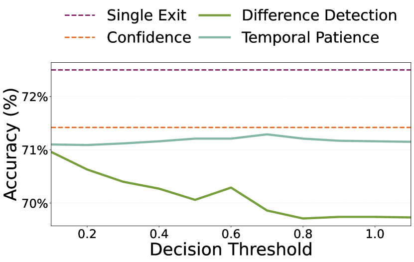
(a) Test Set Accuracy across the threshold configurations for all methods.

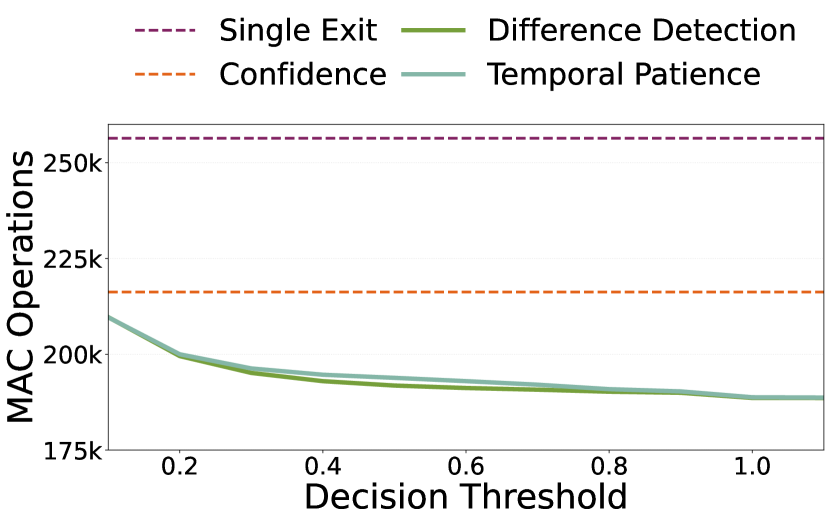
(b) Average MAC ops across the threshold configurations for all methods.

(c) Share of used classifiers for DD EENNs.

(d) Share of used classifiers for TP EENNs.

Figure 3: Benchmark results of a traditional Single Exit Neural Network, an optimized confidence-based EENN, and our novel DD- and TP-EENNs across multiple detection thresholds.

V Difference Detection Early Exit Neural Networks

In existing EENNs, termination of the inference process is typically based on confidence-based metrics, which can lead to errors and vulnerabilities.

To address this issue, we propose a Difference Detection (DD)-based EENN. It leverages the temporal correlation within the sensor data and the propagation of changes through the network architecture to enable more efficient termination decisions.

The DD-EENN calculates the change in the classifier’s output vector as the Euclidean distance between the current classification output vector ($\vec{o}$) and the vector of a previous sample ($\vec{o}_{t_{\text{initial}}}$). This change is defined as the distance ($d$) between the output vectors of the first EE classifier ($\vec{o}_{t,\text{exit}_{0}}$) between samples from two time-steps ($t_{1}$ and $t_{\text{initial}}$) (see Eq. 1).

$$\small\operatorname{change}(t_{1},t_{\text{initial}})=\operatorname{d}(\vec{o}_{t_{1},\text{exit}_{0}},\vec{o}_{t_{\text{initial}},\text{exit}_{0}})\quad,\quad\vec{o}\in\mathbb{R}^{C}$$ (1)

We defined scenes as blocks of consecutive samples that are detected as similar by the decision mechanism. The initial sample of a scene is labeled based on the majority vote of all classifiers, eliminating reliance on unreliable confidence-based metrics (see Eq. 2, where $o_{t,\text{exit}}=\operatorname*{argmax}(\vec{o}_{t,\text{exit}})$ and $n$ is the total number of classifiers in the EENN).

$$\small\operatorname{vote}({o_{t,\text{exit}_{0}},o_{t,\text{exit}_{1}},...,o_{t,\text{exit}_{n}}})=\operatorname*{argmax}_{c\in C}\left(\sum_{i=1}^{n}[o_{t,\text{exit}_{i}}=c]\right)$$ (2)

The prediction at each time step is determined by comparing the currently processed sample to the initial sample. If the change is smaller than the threshold, the prediction of the initial sample is reused, and no deeper layers and classifiers are executed. If the change exceeds the threshold, the prediction is based on the majority vote of all classifiers, indicating the start of a new scene and setting the current sample as new reference (see Eq. 3).

$$\small\operatorname{output}(t)=\begin{cases}\operatorname{vote}_{t_{\text{initial}}}&\text{,if }\operatorname{change}(t,t_{\text{initial}})<\mathrm{threshold}\\ \operatorname{vote}_{t}&\text{,if }\operatorname{change}(t,t_{\text{initial}})\geq\mathrm{threshold}\end{cases}$$ (3)

A similar threshold can be defined for regression tasks to compare the scalar output values of the compared time steps.

By comparing to the initial input of the scene rather than the direct predecessor, mislabeling due to slow drift in subsequent samples is prevented. The use of the early classifier to calculate the change metric improves efficiency by reusing operations between the DD and the inference task. Our approach provides a simple similarity measure for complex radar data without requiring domain knowledge, as in the case of template-matching solutions. This similarity metric approach holds potential for other data modalities, which can be explored in future work.

VI Temporal Patience Early Exit Neural Networks

The DD-EENN relies on the similarity between samples to reuse previous predictions, making its efficiency and accuracy dependent on the defined threshold for an acceptable change. However, always using the first EE classifier in the network and not considering higher-level features extracted by deeper layers can lead to decreased accuracy. To address this, we propose an improved solution with two modifications to enhance accuracy while leveraging the DD approach.

The first adjustment involves the location of the DD EE-classifier in the network architecture. Instead of always using the first classifier, this variant uses the first classifier that agrees with the majority vote of the initial sample of the current sequence for the following inputs of that sequence (see Eq. 4). This allows the mechanism to utilize a classifier more likely to detect a new scene accurately.

$$\small\operatorname{select}(t):=\operatorname*{argmin}_{i}(o_{t,\text{exit}_{i}}=\operatorname{vote}(o_{t,\text{exit}_{0}},o_{t,\text{exit}_{1}},...,o_{t,\text{exit}_{n}}))$$ (4)

The change metric is updated to consider the selected classifier to accommodate this modification. The modified change metric is shown in Eq. 5, where $\vec{o}$ represents the output vectors, $C$ is the number of classes, and $n$ is the selected classifier.

$$\small\operatorname{change}(t,t_{\text{initial}})=\operatorname{d}(\vec{o}_{t,\text{exit}_{i}},\vec{o}_{t_{\text{initial}},\text{exit}_{i}})\quad,\quad\begin{aligned} \vec{o}\in\mathbb{R}^{C}\\ i=\operatorname{select}(t_{\text{initial}})\end{aligned}$$ (5)

The second modification involves using the selected classifier to produce a label for subsequent samples. This reduces reliance on the similarity threshold and adds minimal overhead as the DD’s output vector is already calculated.

These modifications are intended to improve the prediction accuracy but introduce additional computations. Scene change detection now considers the distance between the selected classifier’s output vectors and the label change. This approach incorporates a temporal component inspired by patience-based decision mechanisms. The updated output function at each time step is described by Eq. 6, where the condition determines if the change is within the threshold, and the output is based on the selected classifier or the majority vote.

$$\operatorname{condition}(t) =\operatorname{change}(t,t_{\text{initial}})<\mathrm{threshold}\quad\text{and}$$ (6)

$$\quad\quad\operatorname*{argmax}_{c\in C}(\vec{o}_{t,\text{exit}_{i}})=\operatorname*{argmax}_{c\in C}(\vec{o}_{t_{\text{initial}},\text{exit}_{i}})$$

$$\operatorname{output}(t) =\begin{cases}\vec{o}_{t,\text{exit}_{i}}&\text{, if }\operatorname{condition}(t)\\ \operatorname{vote}(o_{t,\text{exit}_{0}},o_{t,\text{exit}_{1}},\text{...},o_{t,\text{exit}_{n}})&\text{, otherwise}\end{cases}$$

VII Benchmark

To assess the performance of our method, we conducted a benchmark using a private radar dataset. The used test set consists of 237,000 samples that belong to one of five classes as described in section III.

We compared our method to a confidence-based EENN and a Single Exit version of the network architecture as these are the most commonly used methods. The benchmark evaluated test set accuracy and inference efficiency for the people-counting task. During the evaluation, multiple global threshold configurations were explored for our mechanisms, while the confidence-based EENN utilized individual thresholds for each classifier. To measure inference efficiency, we employed the mean of total Multiply-Accumulate (MAC) operations per inference as a hardware-independent metric.

Additionally, we evaluated the majority voting mechanism against the state-of-the-art confidence-based labeling by applying both methods to the entire test set.

VII-A Accuracy

In our benchmark, we compared the EENN decision methods and the Single Exit NN. The Single Exit network achieved the highest accuracy of 72.5 %. The confidence-based EENN achieved the second-highest accuracy of 71.5 %. The DD and TP solutions achieved accuracies ranging from 69.71 % to 70.96 % and 71.12 % to 71.29 %, respectively. Refer to Table  I for the performance of the individual classifiers and the final classifier.

While there was a slight decrease in accuracy, the drops were insignificant in practical applications. The maximum accuracy drop observed was 2.79  percentage point (p.p.) for the DD approach and 1.38 p.p. for the TP approach. Compared to the confidence-based decision mechanism, the maximum accuracy drop was 1.79 p.p. for DD and 0.38 p.p. for TP.

The accuracy of the EENN depends on the accuracy of individual classifiers and the at-runtime decision system. Future work could explore the calibration of exit-wise similarity thresholds to further improve accuracy.

TABLE I: The accuracy and computational cost of the classifiers of the EENN model and the benchmark models.

Model	Single	Conf.	EE1	EE2	Final	Maj.
	Exit	EENN			Class.	Vote
Acc.	72.5 %	71.5 %	69.8 %	71.3 %	72.5 %	71.5 %
MACs	256.3k	216.2k	188.5k	222.2k	256.8k	308.8k

This benchmark highlights the performance of the DD and TP mechanisms, and the detailed accuracies can be found in Fig. 3(a).

VII-B Efficiency

The benchmark evaluated the mean cost in computations as MAC operations per inference on the test set. The Single Exit solution had the highest inference cost of 256 kMAC per sample, while the confidence-based EENN reduced it to 216.26 kMAC (see Fig. 3(b)).

The DD and TP mechanisms significantly reduced the mean inference cost, with both solution achieving a minimum cost of 188.6 kMAC and a maximum cost of 209.7 kMAC. The average cost across all threshold configurations for the DD was 192.8 kMAC and 193.5 kMAC for the TP solution. Compared to the confidence-based solution, these approaches offered inference cost reductions of up to 26 %. The efficiency improvement of the DD and TP solutions came from their execution strategy, where only the earliest or previously selected exit classifier was executed as long as the change between the current and initial samples remained below the threshold. In contrast, confidence-based methods executed all exit calculations until a sufficiently confident result was obtained.

While the TP solution incurred additional costs for a small number of subsequent samples, it showed improved classification capabilities (see Fig. 3(c) and 3(d)). The DD and TP mechanisms demonstrated superior efficiency compared to the confidence-based approach.

VII-C New Scene Labeling

The DD- and TP-EENNs employ a majority voting mechanism for labeling the initial frame of newly detected scenes. This was intended to prevent overthinking - a process in EENNs where EEs produce a correct prediction but are overwritten by deeper classifiers [20]. Comparing the accuracy of the majority voting approach to the confidence-based solution, we found that the majority vote achieved an accuracy of 71.54 %, while the confidence-based approach achieved an accuracy of 71.42 %. The difference between the two approaches was only 0.16 p.p., indicating their similarity in accuracy for this application and that overthinking is not an issue for this application.

Interestingly, we observed that an optimally tuned confidence-based EENN with exit-wise thresholds can compete with the majority vote mechanism in terms of accuracy. This suggests that both approaches have their strengths and weaknesses, and the choice between them may depend on the specific requirements of the task and dataset.

VIII Conclusion

We have introduced a novel approach for processing radar data using EENNs with temporal information. Our evaluation demonstrated significant efficiency gains of up to 26 % compared to the Single Exit network. Both the DD-EENN and TP-EENN solutions are easy to implement and provide cost-effective similarity measurements through computation reuse. While the DD-EENN achieved slightly higher efficiency gains, the TP-EENN maintained higher accuracy across the test set and is less dependent on the threshold hyperparameter configuration. The majority vote and the optimally tuned confidence-based EENN yielded similar accuracies for this use case, indicating the potential for even greater efficiency gains when combining confidence-based labeling for new scenes with the DD approach. Our solution does not require specialized hardware and can be combined with additional optimizations such as quantization and pruning. Future work can focus on utilizing the similarity measurement for additional use cases like monitoring or could evaluate the approach on other data modalities like audio or image data exploring various EENN architectures.

We have shown the possibility of leveraging the temporal correlation of sensor data for more efficient termination decisions on EENNs. This research provides a strong foundation for future work and has the potential to impact various applications.

References

- [1] J.-H. Choi, J.-E. Kim, and K.-T. Kim, “Deep Learning Approach for Radar-Based People Counting,” IEEE Internet of Things Journal, vol. 9, no. 10, pp. 7715–7730, May 2022.
- [2] L. Servadei, H. Sun, J. Ott, M. Stephan, S. Hazra, T. Stadelmayer, D. S. Lopera, R. Wille, and A. Santra, “Label-Aware Ranked Loss for robust People Counting using Automotive in-cabin Radar,” in ICASSP 2022 - 2022 IEEE International Conference on Acoustics, Speech and Signal Processing (ICASSP), May 2022, pp. 3883–3887.
- [3] J. Ott, L. Servadei, G. Mauro, T. Stadelmayer, A. Santra, and R. Wille, “Uncertainty-based Meta-Reinforcement Learning for Robust Radar Tracking,” Oct. 2022.
- [4] G. Mauro, M. De Carlos Diez, J. Ott, L. Servadei, M. P. Cuellar, and D. P. Morales-Santos, “Few-Shot User-Adaptable Radar-Based Breath Signal Sensing,” Sensors, vol. 23, no. 2, p. 804, Jan. 2023.
- [5] G. Mauro, M. Chmurski, L. Servadei, M. Pegalajar-Cuellar, and D. P. Morales-Santos, “Few-Shot User-Definable Radar-Based Hand Gesture Recognition at the Edge,” IEEE Access, vol. 10, pp. 29 741–29 759, 2022.
- [6] T. Zhou, M. Yang, K. Jiang, H. Wong, and D. Yang, “MMW Radar-Based Technologies in Autonomous Driving: A Review,” Sensors, vol. 20, no. 24, p. 7283, Jan. 2020.
- [7] Y. Dong and Y.-D. Yao, “Secure mmWave-Radar-Based Speaker Verification for IoT Smart Home,” IEEE Internet of Things Journal, vol. 8, no. 5, pp. 3500–3511, Mar. 2021.
- [8] P. Panda, A. Sengupta, and K. Roy, “Conditional Deep Learning for energy-efficient and enhanced pattern recognition,” in 2016 Design, Automation & Test in Europe Conference & Exhibition (DATE), Mar. 2016, pp. 475–480.
- [9] B. Fang, X. Zeng, F. Zhang, H. Xu, and M. Zhang, “FlexDNN: Input-Adaptive On-Device Deep Learning for Efficient Mobile Vision,” in 2020 IEEE/ACM Symposium on Edge Computing (SEC), Nov. 2020, pp. 84–95.
- [10] M. Amthor, E. Rodner, and J. Denzler, “Impatient DNNs - Deep Neural Networks with Dynamic Time Budgets,” Oct. 2016.
- [11] H. Hu, D. Dey, M. Hebert, and J. A. Bagnell, “Learning Anytime Predictions in Neural Networks via Adaptive Loss Balancing,” May 2018.
- [12] A. Nguyen, J. Yosinski, and J. Clune, “Deep Neural Networks Are Easily Fooled: High Confidence Predictions for Unrecognizable Images,” in Proceedings of the IEEE Conference on Computer Vision and Pattern Recognition, 2015, pp. 427–436.
- [13] M. Haque, A. Chauhan, C. Liu, and W. Yang, “ILFO: Adversarial Attack on Adaptive Neural Networks,” in Proceedings of the IEEE/CVF Conference on Computer Vision and Pattern Recognition, 2020, pp. 14 264–14 273.
- [14] S. Hong, Y. Kaya, I.-V. Modoranu, and T. Dumitraş, “A Panda? No, It’s a Sloth: Slowdown Attacks on Adaptive Multi-Exit Neural Network Inference,” Feb. 2021.
- [15] M. Wang, Y. D. Zhang, and G. Cui, “Human motion recognition exploiting radar with stacked recurrent neural network,” Digital Signal Processing, vol. 87, pp. 125–131, Apr. 2019.
- [16] J.-W. Choi, S.-J. Ryu, and J.-H. Kim, “Short-Range Radar Based Real-Time Hand Gesture Recognition Using LSTM Encoder,” IEEE Access, vol. 7, pp. 33 610–33 618, 2019.
- [17] M. Scherer, M. Magno, J. Erb, P. Mayer, M. Eggimann, and L. Benini, “TinyRadarNN: Combining Spatial and Temporal Convolutional Neural Networks for Embedded Gesture Recognition With Short Range Radars,” IEEE Internet of Things Journal, vol. 8, no. 13, pp. 10 336–10 346, Jul. 2021.
- [18] S. Hazra and A. Santra, “Short-Range Radar-Based Gesture Recognition System Using 3D CNN With Triplet Loss,” IEEE Access, vol. 7, pp. 125 623–125 633, 2019.
- [19] E. Park, D. Kim, S. Kim, Y.-D. Kim, G. Kim, S. Yoon, and S. Yoo, “Big/little deep neural network for ultra low power inference,” in 2015 International Conference on Hardware/Software Codesign and System Synthesis (CODES+ISSS), Oct. 2015, pp. 124–132.
- [20] Y. Kaya, S. Hong, and T. Dumitras, “Shallow-Deep Networks: Understanding and Mitigating Network Overthinking,” in Proceedings of the 36th International Conference on Machine Learning. PMLR, May 2019, pp. 3301–3310.
- [21] T. Bolukbasi, J. Wang, O. Dekel, and V. Saligrama, “Adaptive Neural Networks for Efficient Inference,” in Proceedings of the 34th International Conference on Machine Learning. PMLR, Jul. 2017, pp. 527–536.
- [22] A. Odena, D. Lawson, and C. Olah, “Changing Model Behavior at Test-Time Using Reinforcement Learning,” Feb. 2017.
- [23] M. Sabih, F. Hannig, and J. Teich, “DyFiP: Explainable AI-based dynamic filter pruning of convolutional neural networks,” in Proceedings of the 2nd European Workshop on Machine Learning and Systems, ser. EuroMLSys ’22. New York, NY, USA: Association for Computing Machinery, Apr. 2022, pp. 109–115.
- [24] W. Zhou, C. Xu, T. Ge, J. McAuley, K. Xu, and F. Wei, “BERT Loses Patience: Fast and Robust Inference with Early Exit,” in Advances in Neural Information Processing Systems, vol. 33. Curran Associates, Inc., 2020, pp. 18 330–18 341.
- [25] N. Rashid, B. U. Demirel, M. Odema, and M. A. Al Faruque, “Template Matching Based Early Exit CNN for Energy-efficient Myocardial Infarction Detection on Low-power Wearable Devices,” Proceedings of the ACM on Interactive, Mobile, Wearable and Ubiquitous Technologies, vol. 6, no. 2, pp. 68:1–68:22, Jul. 2022.
- [26] R. David, J. Duke, A. Jain, V. Janapa Reddi, N. Jeffries, J. Li, N. Kreeger, I. Nappier, M. Natraj, T. Wang, P. Warden, and R. Rhodes, “Tensorflow lite micro: Embedded machine learning for tinyml systems,” in Proceedings of Machine Learning and Systems, A. Smola, A. Dimakis, and I. Stoica, Eds., vol. 3, 2021, pp. 800–811.
- [27] F. Chollet, “Xception: Deep learning with depthwise separable convolutions,” in Proceedings of the IEEE conference on computer vision and pattern recognition, 2017, pp. 1251–1258.