On the quality of randomized approximations of Tukey’s depth

Abstract

Tukey’s depth (or halfspace depth) is a widely used measure of centrality for multivariate data. However, exact computation of Tukey’s depth is known to be a hard problem in high dimensions. As a remedy, randomized approximations of Tukey’s depth have been proposed. In this paper we explore when such randomized algorithms return a good approximation of Tukey’s depth. We study the case when the data are sampled from a log-concave isotropic distribution. We prove that, if one requires that the algorithm runs in polynomial time in the dimension, the randomized algorithm correctly approximates the maximal depth $1/2$ and depths close to zero. On the other hand, for any point of intermediate depth, any good approximation requires exponential complexity.

1 Introduction

Ever since Tukey introduced a notion of data depth [44], it has been an important tool of data analysts to measure centrality of data points in multivariate data. Apart from Tukey’s depth (also called halfspace depth), many other depth measures have been developed, such as simplical depth (Liu [28, 29]), projection depth (Liu [30], Zuo and Serfling [46]), a notion of “outlyingness” (Stahel [43], Donoho [13]), and the zonoid depth (Dyckerhoff et al. [16], Koshevoy and Mosler [25]). Each of these notions offer distinct stability and computability properties that make them suitable for different applications (Mosler and Mozharovskyi [34]). For surveys of depth measures and their applications we refer the reader to Mosler [33], Aloupis [1], Dyckerhoff and Mozharovskyi [15], and Nagy et al. [35].

Tukey’s depth is defined as follows: for $x\in\mathbb{R}^{d}$ and unit vector $u\in S^{d-1}$ (where $S^{d-1}$ is the unit sphere of $\mathbb{R}^{d}$ under the euclidean norm), introduce the closed half space

$$H(x,u)=\left\{y\in\mathbb{R}^{d}\ :\ \langle y,u\rangle\leq\langle x,u\rangle\right\}~{},$$

where $\langle\cdot,\cdot\rangle$ is the usual scalar product on $\mathbb{R}^{d}$. Given a set of $n$ data points $\{x_{1},\ldots,x_{n}\}$ in $\mathbb{R}^{d}$, for each $x\in\mathbb{R}^{d}$, define the directional depth

$$r_{n}(x,u)=\frac{1}{n}\sum_{i=1}^{n}\mathbbm{1}_{x_{i}\in H(x,u)}~{}.$$

The depth of $x$ in the point set $\{x_{1},\ldots,x_{n}\}$ is defined as

$$d_{n}(x)=\inf_{u\in S^{d-1}}r_{n}(x,u)~{}.$$

Note that, due to the normalization in our definition, $d_{n}(x)\in[0,1/2]$ for all $x\in\mathbb{R}^{d}$. Tukey’s depth possesses properties expected of a depth measure. It is affine invariant, it vanishes at infinity, and it is monotone decreasing on rays emanating from the deepest point. It is also robust under a symmetry assumption (Donoho and Gasko [14]).

A well-known disadvantage of Tukey’s depth is that even its approximate computation is known to be a np-hard problem (Amaldi and Kann [2], Bremner et al. [5], Johnson and Preparata [21]), presenting challenges for applications. While fast algorithms exist for computing the depth of the deepest point in two dimensions (Chan [8]), the computational complexity grows exponentially with the dimension. Chan [8] gives a maximum-depth computation algorithm of complexity $\mathcal{O}(n^{d-1})$.

The curse of dimensionality affects several other depth measures, posing significant challenges in multivariate analysis. To address these challenges, focus has been put on developing approximation algorithms. Dyckerhoff et al. [17] emphasize the importance of finding such algorithms and Shao et al. [42] propose mcmc methods for approximating the projection depth. Zuo [45] suggests an approximate version of Tukey’s depth and provides an algorithm with linear time complexity in the dimension, though the proposed version may be a poor approximation of Tukey’s depth.

A natural way of approximating Tukey’s depth, proposed by Cuesta-Albertos and Nieto-Reyes [11], is a randomized version in which the infimum over all possible directions $u\in S^{d-1}$ in the definition of $d_{n}(x)$ is replaced by the minimum over a number of randomly chosen directions. More precisely, let $U_{1},\ldots,U_{k}$ be independent identically distributed vectors sampled uniformly on the unit sphere $S^{d-1}$, and define the random Tukey depth (with respect to the point set $\{x_{1},\ldots,x_{n}\}$) as

$$D_{n,k}(x)=\min_{i=1,\ldots,k}r_{n}(x,U_{i})~{}.$$

It is easy to see that for every $x\in\mathbb{R}^{d}$, $\lim_{k\to\infty}D_{n,k}(x)=d_{n}(x)$ with probability $1$. However, this randomized approach is only useful if the number of random directions $k$ is reasonably small so that computation is feasible. The purpose of this paper is to explore the tradeoff between computational complexity and accuracy. In particular, we may ask how large $k$ has to be in order to guarantee that, for given accuracy and confidence parameters $\epsilon\in(0,1/2)$ and $\delta\in(0,1)$, $|D_{n,k}(x)-d_{n}(x)|\leq\epsilon$ with probability at least $1-\delta$.

It is easy to see that the value of $k$ required to satisfy the property above may be arbitrarily large. To see this, consider the two-dimensional example in which, for $i=1,\ldots,n$, the points $x_{i}=(x_{i,1},x_{i,2})$ are defined by

$$x_{i,1}=\frac{i}{n}~{},\qquad x_{i,2}=a\left(\frac{i}{n}\right)^{2}$$

where $a>0$ is a parameter. For any $k$, as $a\to 0$, the random depth fails to approximate $d_{n}(x_{n/2})=1/n$.

In order to exclude the anomalous behavior of the example above, we assume that the points $x_{i}$ are drawn randomly from an isotropic log-concave distribution $\mu$. Recall that a distribution $\mu$ is log-concave if it is absolutely continuous with respect to the Lebesgue measure, with density $f$ of the form $f(x)=e^{-g(x)}$ where $g:\mathbb{R}^{d}\to\mathbb{R}$ is a convex function. $\mu$ is isotropic if for a random vector $X$ distributed by $\mu$, the covariance matrix $\mathbb{E}(X-\mathbb{E}X)(X-\mathbb{E}X)^{T}$ is the identity matrix. Examples of log-concave distributions include Gaussian distributions and the uniform distribution on a convex body in $\mathbb{R}^{d}$.

For random data, one may introduce the “population” counterpart of $r_{n}$ defined by

$$\overline{r}(x,u)=\mu(H(x,u))~{}.$$

Similarly, the population versions of the Tukey depth and randomized Tukey depth are defined by

$$\overline{d}(x)=\inf_{u\in S^{d-1}}\overline{r}(x,u)\quad\mbox{and}\quad\overline{D}_{k}(x)=\min_{i=1,\ldots,k}\overline{r}(x,U_{i})~{}.$$

As it was observed by Cuesta-Albertos and Nieto-Reyes [11] and Chen et al. [10], as long as $n\gg d$, the population versions of the Tukey depth $\overline{d}(x)$ and randomized Tukey depth $\overline{D}_{k}(x)$ are good approximations of $d_{n}(x)$ and $D_{n,k}(x)$, respectively. This follows from standard uniform convergence results of empirical process theory based on the vc dimension. The next lemma quantifies this closeness. For completeness we include its proof in the Appendix.

Lemma 1

Let $\delta>0$. If $X_{1},\ldots,X_{n}$ are independent, identically distributed random vectors in $\mathbb{R}^{d}$, then

$$\mathbb{P}\left\{\sup_{x\in\mathbb{R}^{d}}|\overline{d}(x)-d_{n}(x)|\geq c\sqrt{\frac{d}{n}}+\sqrt{\frac{\log(1/\delta)}{2n}}\right\}\leq\delta$$

where $c$ is a universal constant. Also, given any fixed values of $U_{1},\ldots,U_{k}$,

$$\mathbb{P}\left\{\left.\sup_{x\in\mathbb{R}^{d}}|\overline{D}_{k}(x)-D_{n,k}(x)|\geq c\sqrt{\frac{\min(d,\log(k))}{n}}+\sqrt{\frac{\log(1/\delta)}{2n}}\right|U_{1},\ldots,U_{k}\right\}\leq\delta$$

Thanks to Lemma 1, in the rest of the paper we restrict our attention to the population quantities $\overline{d}(x)$ and $\overline{D}_{k}(x)$ and we may forget the data points $X_{1},\ldots,X_{n}$. In particular, we are interested in finding out for what points $x\in\mathbb{R}^{d}$ and $k\geq 0$ the random Tukey depth $\overline{D}_{k}(x)$ is a good approximation of $\overline{d}(x)$. To this end, we fix an accuracy $\epsilon>0$ and a confidence level $\delta>0$ and ask that

$$\overline{D}_{k}(x)-\overline{d}(x)\leq\epsilon\quad\text{holds with probability at least $1-\delta$}.$$ (1)

(Note that, by definition, $\overline{D}_{k}(x)\geq\overline{d}(x)$ for all $x$ and $k$.) The main results of the paper show an interesting trichotomy: for most “shallow” points (i.e., those with $\overline{d}(x)\leq\epsilon$), we have $\overline{D}_{k}(x)\leq\epsilon$ with probability at least $1-\delta$ even for $k$ of constant order, depending only on $\epsilon$ and $\delta$. When $x$ has near maximal depth in the sense that $\overline{d}(x)\approx 1/2$ (note that such points may not exist unless the density of $\mu$ is symmetric around $0$), then for values of $k$ that are slightly larger than a linear function of $d$, (1) holds. However, in sharp contrast with this, for points $x$ of intermediate depth, $k$ needs to be exponentially large in $d$ in order to guarantee (1). Hence, roughly speaking, the depth of very shallow and very deep points can be efficiently approximated by the random Tukey depth but for all other points, any reasonable approximation by the random Tukey depth requires exponential complexity.

1.1 Related literature

Cuesta-Albertos and Nieto-Reyes [11] explore various properties of the random Tukey depth and report good experimental behavior. The maximum discrepancy between $d_{n}$ and its randomized approximation has also been studied by Nagy et al. [36]. They establish conditions under which $\sup_{x\in\mathbb{R}^{d}}\left(\overline{D}_{k}(x)-\overline{d}(x)\right)\to 0$ as $k\to\infty$ and provide bounds for the rate of convergence. As opposed to the global view of [36], our aim is to identify the points $x$ for which the random Tukey depth approximates well $\overline{d}(x)$ for values of $k$ that are polynomial in the dimension.

Brazitikos et al. [4] show that the average depth $\int\overline{d}(x)d\mu(x)$ is exponentially small in the dimension when $\mu$ is log-concave.

Brunel [7] studies convergence of the empirical level sets when the data points are drawn independently from the same distribution.

Chen et al. [9] study the quality of other randomized approximations of the Tukey depth for point sets in general position.

1.2 Contributions and outline

As mentioned above, the main results of this paper show that, for isotropic log-concave distributions, the quality of approximation of the random Tukey depth varies dramatically, depending on the depth of the point $x$.

Most points have a small random Tukey depth

In Section 2 we establish results related to shallow points. It follows from results of Brazitikos et al. [4] and Markov’s inequality that all but an exponentially small fraction of points are shallow in the sense that, for all $\epsilon>0$,

$$\mu\left(\left\{x\in\mathbb{R}^{d}:\overline{d}(x)>\epsilon\right\}\right)\leq\frac{e^{-cd}}{\epsilon}~{},$$

where $c>0$ is a universal constant. The main result of Section 2 is that, in high dimensions, not only most points are shallow but most points even have a small random Tukey depth for $k$ of constant order, only depending on the desired accuracy. In particular, Theorem 5 implies the following.

Of course, $\overline{D}_{k}(x)\leq\epsilon$ implies that $\overline{d}(x)\leq\epsilon$ and, in particular, that $\overline{D}_{k}(x)-\overline{d}(x)\leq\epsilon$. Thus, Corollary 2 implies that the random Tukey depth of most points (in terms of the measure $\mu$) is a good approximation of the Tukey depth after taking just a constant number of random directions. All of these points are shallow in the sense that $\overline{d}(x)\leq\epsilon$.

It is natural to ask whether the Tukey depth of every shallow point is well approximated by its random version. However, this is false as the following example shows.

Example. Let $\mu$ be the uniform distribution on $[-(3/2)^{1/3},(3/2)^{1/3}]^{d}$ so that $\mu$ is isotropic and log-concave on $\mathbb{R}^{d}$. If $x=((3/2)^{1/3},0,\ldots,0)$, then $\overline{d}(x)=0$, but it is a simple exercise to show that $\overline{D}_{k}\geq 1/4$ with high probability, unless $k$ is exponentially large in $d$.

Intermediate depth is hard to approximate

Arguably the most interesting points are those whose depth is in the intermediate range, bounded away from $0$ and $1/2$. Unfortunately, for all such points, the random Tukey depth is an inefficient approximation of the Tukey depth. In Section 3 we show that for all points in this range, the random Tukey depth $\overline{D}_{k}(x)$ is close to $1/2$, with high probability, unless $k$ is exponentially large in the dimension. Hence, in high dimensions, $\overline{D}_{k}(x)$ fails to efficiently approximate the true depth $\overline{d}(x)$. In particular, Theorem 8 implies the following.

Points of maximum depth are easy to localize

As mentioned above, the Tukey depth $\overline{d}(x)$ of any $x\in\mathbb{R}^{d}$ is at most $1/2$. If $\overline{d}(x)=1/2$, then for every $u\in S^{d-1}$, the median of the projection $\langle X,u\rangle$ equals $\langle x,u\rangle$ (where the random vector $X$ is distributed as $\mu$). Such points are quite special and may not exist at all. If there exists an $x\in\mathbb{R}^{d}$ with $\overline{d}(x)=1/2$, then the measure $\mu$ is called halfspace symmetric (see Zuo and Serfling [47], Nagy et al. [35]). It is easy to see that if $\mu$ is halfspace symmetric, there is a unique $m\in\mathbb{R}^{d}$ with $\overline{d}(m)=1/2$. We call $m$ the Tukey median of $\mu$. Centrally symmetric measures are halfspace symmetric though the converse does not hold in general. Remarkably, if $\mu$ is the uniform distribution over a convex body and it is halfspace symmetric, then it is also centrally symmetric, see Funk [19], Schneider [41].

We note that for any log-concave measure, $1/e\leq\sup_{x\in\mathbb{R}^{d}}\overline{d}(x)\leq 1/2$, see Nagy et al. [35, Theorem 3].

If $m\in\mathbb{R}^{d}$ is such that $\overline{d}(m)=1/2$, then clearly $\overline{D}_{k}(m)=1/2$ for all $k\geq 1$. In Section 4 we show that, for values of $k$ that are only polynomial in $d$, points with $\overline{D}_{k}(x)\approx 1/2$ must be close to $x$. Hence, the random Tukey depth efficiently estimates the Tukey median for halfspace symmetric isotropic log-concave distributions. More precisely, Theorem 9, combined with Lemma 1 implies the following.

By taking $\gamma$ of the order of $1/\sqrt{d}$, the corollary above shows that, as long as $n\gg d^{2}$, it suffices to take $O(d\log d)$ random directions so that the empirical random Tukey median is within distance of constant order of the Tukey median. Note that, due to the “thin-shell” property of log-concave measures (see, e.g., [18]), the measure $\mu$ is concentrated around a sphere of radius $\sqrt{d}$ centered at the Tukey median $m$ and hence localizing $m$ to within a constant distance is a nontrivial estimate.

One may even take $\gamma$ to be smaller order than $1/\sqrt{d}$ and get a better precision with the same value of $k$. However, for better precision, one requires the sample size $n$ to be larger.

2 Random Tukey depth of typical points

In this section we show that for isotropic log-concave distributions, in high dimensions, a constant number $k$ of random directions suffice to make the random Tukey depth $\overline{D}_{k}$ small for most points. In other words, the curse of dimensionality is avoided in a strong sense. In particular, we prove the following theorem that implies Corollary 2 in a straightforward manner.

Theorem 5

Assume that $\mu$ is an isotropic log-concave measure on $\mathbb{R}^{d}$. There exist universal constants $c,\kappa>0$ such that the following holds. Let $\epsilon>0$ and suppose that $d$ is so large that $d^{-\kappa}\leq\epsilon/2$. Then for every $k\leq cd^{\kappa}$,

$$\mu\left(\{x\in\mathbb{R}^{d}:\overline{D}_{k}(x)>\epsilon\}\right)\leq(1-\epsilon/4)^{k}+(k+1)d^{-\kappa}+ke^{\frac{-d\pi}{64\log(1/\epsilon)k}}$$

with probability at least $1-ke^{-ck}-3ke^{-c\sqrt{d}}$ over the choice of directions $U_{1},\dots,U_{k}$.

Our main tool is the following extension of Klartag’s celebrated central limit theorem for convex bodies (Klartag [22]). Let $G_{d,k}$ denote the grassmannian of all $k$-dimensional subspaces of $\mathbb{R}^{d}$ and let $\sigma_{d,k}$ be the unique rotationally invariant probability measure on $G_{d,k}$.

Proposition 6

(Klartag [23].) Let the random vector $X$ take values in $\mathbb{R}^{d}$ and assume that $X$ has an isotropic log-concave distribution. Let $S_{k}$ be a random $k$-dimensional subspace of $\mathbb{R}^{d}$ drawn from the distribution $\sigma_{d,k}$. There exist universal constants $c,\kappa>0$ such that the following holds: if $k\leq cd^{\kappa}$, then with probability at least $1-e^{-c\sqrt{d}}$, for every measurable set $A\subset S_{k}$,

$$\left|\mathbb{P}\{\pi_{k}(X)\in A\}-\mathbb{P}\{N\in A\}\right|\leq d^{-\kappa}$$

where $N$ is a $k$-dimensional normal vector in $S_{k}$ with zero mean and identity covariance matrix, and $\pi_{k}$ is the orthogonal projection on $S_{k}$.

Proof of Theorem 5: First note that the random subspace of $\mathbb{R}^{d}$ spanned by the independent uniform vectors $U_{1},\ldots,U_{k}$ has a rotation-invariant distribution and therefore it is distributed by $\sigma_{d,k}$ over the grassmannian $G_{d,k}$.

For any $u\in S^{d-1}$, define $q(\epsilon,u)$ as the $\epsilon$-quantile of the distribution of $\langle X,u\rangle$, that is,

$$\mu(\{x:\langle x,u\rangle\leq q(\epsilon,u)\})=\epsilon~{}.$$

Observe that, by Proposition 6 (applied with $k=1$) and the union bound, with probability at least $1-ke^{-c\sqrt{d}}$,

$$\mbox{for all $i=1,\ldots,k$,}\quad q(\epsilon,U_{i})\geq\Phi^{-1}(\epsilon/2)$$

whenever $d$ is so large that $d^{-\kappa}\geq\epsilon/2$ where $\Phi(z)=\int_{-\infty}^{z}(2\pi)^{-1/2}e^{-x^{2}/2}dx$ denotes the standard Gaussian cumulative distribution function.

Then, with probability at least $1-ke^{-c\sqrt{d}}$,

$$\mu\left(\left\{x:\overline{D}_{k}(x)>\epsilon\right\}\right) = \mu\left(\left\{x:\min_{i=1,\ldots,k}\mu(H(x,U_{i}))>\epsilon\right\}\right)$$

$$= \mu\left(\left\{x:\langle x,U_{i}\rangle>q(\epsilon,U_{i})\ \mbox{for all $i=1,\ldots,k$}\right\}\right)$$

$$\leq \mu\left(\left\{x:\langle x,U_{i}\rangle>\Phi^{-1}(\epsilon/2)\ \mbox{for all $i=1,\ldots,k$}\right\}\right)$$

If the $U_{i}$ were orthogonal, we could now use Proposition 6. This is not the case but almost. In order to handle this issue, we perform Gram-Schmidt orthogonalization defined, recursively, by $V_{1}=U_{1}$ and, for $i=2,\ldots,k$,

$$R_{i}=\sum_{j=1}^{i-1}\langle U_{i},V_{j}\rangle V_{j}\quad\mbox{and}\quad V_{i}=\frac{U_{i}-R_{i}}{\|U_{i}-R_{i}\|}~{}.$$

Then $V_{1},\ldots,V_{k}$ are orthonormal vectors, spanning the same subspace as $U_{1},\ldots,U_{k}$.

Now, we may write

$$\mu\left(\left\{x:\overline{D}_{k}(x)>\epsilon\right\}\right)$$ (2)

$$\leq \mu\left(\left\{x:\langle x,U_{i}\rangle>\Phi^{-1}(\epsilon/2)\ \mbox{for all $i=1,\ldots,k$}\right\}\right)$$

$$\leq \mu\left(\left\{x:\langle x,V_{i}\rangle>\Phi^{-1}(\epsilon/4)\ \mbox{for all $i=1,\ldots,k$}\right\}\right)$$

$$+\mu\left(\left\{x:\langle x,U_{i}-V_{i}\rangle>\Phi^{-1}(\epsilon/2)-\Phi^{-1}(\epsilon/4)\ \mbox{for some $i=1,\ldots,k$}\right\}\right)$$

$$\leq \mu\left(\left\{x:\langle x,V_{i}\rangle>\Phi^{-1}(\epsilon/4)\ \mbox{for all $i=1,\ldots,k$}\right\}\right)$$

$$+\sum_{i=1}^{k}\mu\left(\left\{x:\langle x,U_{i}-V_{i}\rangle>\frac{\sqrt{2\pi}}{4\log(1/\epsilon)}\right\}\right)~{},$$

where the last inequality follows from the union bound and the inequality

$$\Phi^{-1}(\epsilon/2)-\Phi^{-1}(\epsilon/4)\geq\frac{\sqrt{2\pi}}{4\log(1/\epsilon)}~{}.$$ (3)

Indeed, since $\Phi^{-1}$ is concave, we have

$$\frac{\Phi^{-1}(\epsilon/2)-\Phi^{-1}(\epsilon/4)}{\epsilon/4}\geq(\Phi^{-1})^{\prime}(\epsilon/2)~{}.$$

Using the fact that $(\Phi^{-1})^{\prime}=1/(\Phi^{\prime}\Phi^{-1})$ and $\Phi^{\prime}(t)=\frac{1}{\sqrt{2\pi}}e^{-t^{2}/2}$,

$$\Phi^{-1}(\epsilon/2)-\Phi^{-1}(\epsilon/4)\geq\frac{\epsilon}{4}\sqrt{2\pi}e^{\Phi^{-1}(\epsilon/2)^{2}/2}~{}.$$ (4)

By Gordon’s inequality for the Mills’ ratio (Gordon [20]), for $t\leq 0$,

$$\Phi(t)\geq-\frac{1}{\sqrt{2\pi}}\frac{t}{t^{2}+1}e^{-t^{2}/2}~{},$$

and therefore

$$t\geq\Phi^{-1}\left(-\frac{1}{\sqrt{2\pi}}\frac{t}{t^{2}+1}e^{-t^{2}/2}\right)~{},$$

leading, for $t<-1$, to

$$t\geq\Phi^{-1}\left(-\frac{e^{-t^{2}/2}}{10t}\right)~{}.$$ (5)

Choosing $t_{\epsilon}=-\sqrt{2\log(1/\epsilon)}\sqrt{1-\frac{\log\log(1/\epsilon)}{\log(1/\epsilon)}}$ for $\epsilon<e^{-2}$ and noting that

$$-\frac{e^{-t_{\epsilon}^{2}/2}}{10t_{\epsilon}}\geq\epsilon/2,$$

(5) implies that

$$-\sqrt{2\log(1/\epsilon)}\sqrt{1-\frac{\log\log(1/\epsilon)}{\log(1/\epsilon)}}\geq\Phi^{-1}(\epsilon/2)~{}.$$

Plugging this inequality into (4)

$$\Phi^{-1}(\epsilon/2)-\Phi^{-1}(\epsilon/4)\geq\frac{\sqrt{2\pi}}{4\log(1/\epsilon)}~{},$$

proving (3).

As $\langle x,V_{1}\rangle,\ldots,\langle x,V_{k}\rangle$ are coordinates of the orthogonal projection of $x$ on the random subspace spanned by $U_{1},\ldots,U_{k}$, we may use Proposition 6 to bound the first term on the right-hand side of (2). Let $N_{1},\ldots,N_{k}$ be independent standard normal random variables. Then by Proposition 6, with probability at least $1-e^{-c\sqrt{d}}$,

$$\mu\left(\left\{x:\langle x,V_{i}\rangle>\Phi^{-1}(\epsilon/4)\ \mbox{for all $i=1,\ldots,k$}\right\}\right)$$

$$\leq \mathbb{P}\{N_{i}>\Phi^{-1}(\epsilon/4)\ \mbox{for all $i=1,\ldots,k$}\}+d^{-\kappa}$$

$$= \mathbb{P}\{N_{1}>\Phi^{-1}(\epsilon/4)\}^{k}+d^{-\kappa}$$

$$= (1-\epsilon/4)^{k}+d^{-\kappa}$$

It remains to bound the second term on the right-hand side of (2). Once again, we use Proposition 6. By rotational invariance, the distribution of $U_{i}-V_{i}/\|U_{i}-V_{i}\|$ is uniform on $S^{d-1}$ and therefore the distribution of $\mu\left(\left\{x:\langle x,U_{i}-V_{i}\rangle>\frac{\sqrt{2\pi}}{4\log(1/\epsilon)}\right\}\right)$ is the same as that of

$$\mu\left(\left\{x:\langle x,W\rangle>\frac{\sqrt{2\pi}}{4\log(1/\epsilon)\|U_{i}-V_{i}\|}\right\}\right)$$

(if $\epsilon\leq 1/2$) where $W$ is uniformly distributed on $S^{d-1}$, independent of $U_{1},\ldots,U_{n}$. .By Lemma 7 below, with probability at least $1-ke^{-ck}$,

$\max_{i=1,\ldots,k}\|U_{i}-V_{i}\|\leq\sqrt{4k/d}$.

Combining this with Proposition 6, we have that, with probability at least $1-ke^{-ck}-ke^{-c\sqrt{d}}$,

$$\sum_{i=1}^{k}\mu\left(\left\{x:\langle x,U_{i}-V_{i}\rangle>\frac{\sqrt{2\pi}}{4\log(1/\epsilon)}\right\}\right) \leq kd^{-\kappa}+k\mathbb{P}\left\{N>\frac{\sqrt{2\pi}}{4\log(1/\epsilon)}\sqrt{\frac{d}{4k}}\right\}$$

$$\leq kd^{-\kappa}+ke^{\frac{-d\pi}{64\log(1/\epsilon)k}}~{}.$$

In order to complete the proof of Theorem 5, it remains to prove the following simple inequality.

Lemma 7

For every $i=1,\ldots,k$, with probability at least $1-e^{-ck}$,

$$\|U_{i}-V_{i}\|\leq\sqrt{\frac{4k}{d}}$$

where $c$ is a universal constant.

Proof: Note that, since $\|R_{i}\|^{2}=\langle U_{i},R_{i}\rangle$,

$$\langle U_{i},V_{i}\rangle=\frac{1-\langle U_{i},R_{i}\rangle}{\|U_{i}-R_{i}\|}=\sqrt{1-\|R_{i}\|^{2}}\leq 1-\|R_{i}\|^{2}$$

and therefore

$$\|U_{i}-V_{i}\|^{2}=2(1-\langle U_{i},V_{i}\rangle)\leq 2\|R_{i}\|^{2}=2\sum_{j=1}^{i-1}\langle U_{i},V_{j}\rangle^{2}~{}.$$

We may write $U_{i}=Z_{i}/\|Z_{i}\|$ where $Z_{i}$ is a Gaussian vector in $\mathbb{R}^{d}$ with zero mean and identity covariance matrix. Since $Z_{i}$ is independent of $V_{1},\ldots,V_{i-1}$ and the $V_{j}$ are orthonormal, $\sum_{j=1}^{i-1}\langle Z_{i},V_{j}\rangle^{2}$ is a $\chi^{2}$ random variable with $i-1$ degrees of freedom. Thus, $\|U_{i}-V_{i}\|^{2}$ is the ratio of a $\chi^{2}(i-1)$ and a $\chi^{2}(d)$ random variable (which are not independent). By standard tail bounds of the $\chi^{2}$ distribution (see, e.g., [3]), with probability at least $1-e^{-ck}$,

$$\|U_{i}-V_{i}\|^{2}\leq\frac{4k}{d}~{}.$$

$\Box$

3 Estimating intermediate depth is costly

In this section we prove that, even though the random Tukey depth is small for most points $x\in\mathbb{R}^{d}$ (according to the measure $\mu$), whenever the depth $\overline{d}(x)$ of a point is not small, its random Tukey depth $\overline{D}_{k}(x)$ is close to $1/2$, unless $k$ is exponentially large in $d$. This implies that for points whose depth is bounded away from $1/2$, the random Tukey depth is a poor approximation of $\overline{d}(x)$.

The main result of the section is the following theorem that immediately implies Corollary 3 stated in Section 1.

Theorem 8

Assume that $\mu$ is an isotropic log-concave measure on $\mathbb{R}^{d}$ and let $0<\gamma<1/2$. Let $x\in\mathbb{R}^{d}$ be such that $\overline{d}(x)=\gamma$ and let $\epsilon>0$. Then

$$\mathbb{P}\left\{\overline{D}_{k}(x)\leq\frac{1}{2}-C_{\gamma}\frac{\epsilon}{\log\left(\frac{1}{\epsilon}\right)}\right\}\leq 2ke^{-(d-1)\epsilon^{2}/2}~{},$$

where $C_{\gamma}>0$ is a constant depending only on $\gamma$.

Proof: Without loss of generality, we may assume that the origin has maximal depth, that is, $\overline{d}(0)=\sup_{x\in\mathbb{R}^{d}}\overline{d}(x)$. Fix $x\in\mathbb{R}^{d}$ with $\overline{d}(x)=\gamma$, and note that $\overline{d}(0)\geq\gamma$.

The main tool of this proof is Lévy’s isoperimetric inequality (Schmidt [40], Lévy [27], see also Ledoux [26]). It states that if the random vector $U$ is uniformly distributed on the sphere $S^{d-1}$ and $A$ a is Borel-measurable set such that $\mathbb{P}\{U\in A\}\geq 1/2$, then for any $\epsilon>0$,

$$\mathbb{P}\left\{\inf_{v\in A}\|U-v\|\geq\epsilon\right\}\leq 2e^{-(d-1)\epsilon^{2}/2}~{}.$$ (6)

Lévy’s inequality may be used to prove concentration inequalities for smooth functions of the random vector $U$. Our goal is to prove that the measure $\mu(H(x,U))$ of the random halfspace $H(x,U)$ is concentrated around its median $1/2$.

In order to prove smoothness of the function $\mu(H(x,u))$ (as a function of $u\in S^{d-1}$), fix $u,v\in S^{d-1}$, $u\neq v$. Consider the $2$-dimensional cone spanned by the segments $(x,u)$ and $(x,v)$ defined by

$$C(x,u,v)=\left\{x+au+bv:\ a,b\in\mathbb{R}^{+}\right\}~{}.$$

Denote by $\mathcal{H}$ the only two-dimensional affine space containing $x,\ x+u,\ x+v$.

We also define $P_{\mathcal{H}}$ as the orthogonal projection onto $\mathcal{H}$. Denoting by $\widetilde{\mu}=P_{\mathcal{H}}\#\mu$ and $\widetilde{H}(x,u)=P_{\mathcal{H}}\left(H(x,u)\right)$, we have

$$\mu(H(x,u))=\widetilde{\mu}\left(\widetilde{H}(x,u)\right)~{}.$$

Thus, after projecting on the plane $\mathcal{H}$, it suffices to control

$$|\mu(H(x,u))-\mu(H(x,v))| = \left|\widetilde{\mu}\left(\widetilde{H}(x,u)\right)-\widetilde{\mu}\left(\widetilde{H}(x,v)\right)\right|$$ (7)

$$= \left|\widetilde{\mu}\left(C(x,u^{\perp},v^{\perp})\right)-\widetilde{\mu}\left(C(x,-u^{\perp},-v^{\perp})\right)\right|$$

$$\leq \widetilde{\mu}\left(C(x,u^{\perp},v^{\perp})\right)+\widetilde{\mu}\left(C(x,-u^{\perp},-v^{\perp})\right)~{},$$

that is, the measure of two cones in a $2$ dimensional affine space. Here, given an arbitrary orientation to the plane $\mathcal{H}$, $u^{\perp}$ and $v^{\perp}$ are the only unit vectors orthogonal to $u$ and $v$, respectively, in $\mathcal{H}$ such that $u^{\perp}$ and $v^{\perp}$ are rotated $90$ degrees counter-clockwise from $u$ and $v$, see Figure 1.

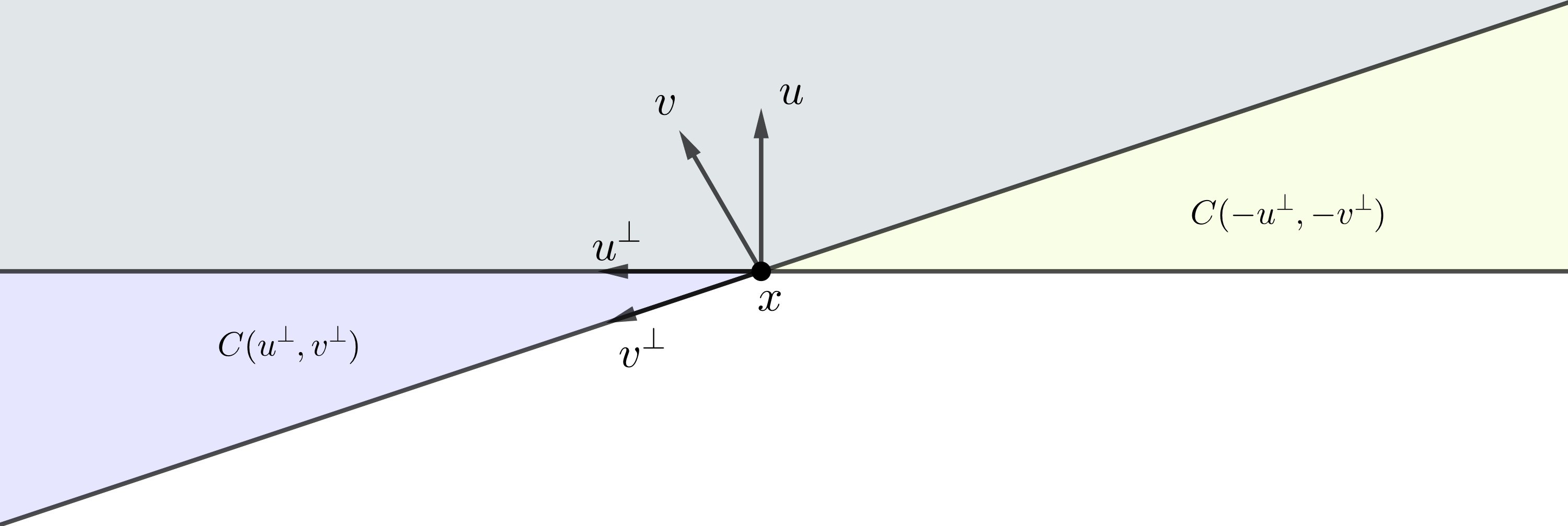
Figure 1: Illustration of the cones $C(x,u^{\perp},v^{\perp})$ and $C(x,-u^{\perp},-v^{\perp})$.

Since the measure $\widetilde{\mu}$ is itself an isotropic log-concave measure (see Saumard and Wellner [39, Section 3], Prékopa [37]), the problem becomes two dimensional. Next, we show that neither $\|x\|$ nor $|m_{v}|$ are too large, where $m_{v}$ denotes the median of the random variable $\langle X,v\rangle$. (Note that $m_{v}$ is uniquely defined since $\langle X,v\rangle$ is log-concave and therefore has a unimodal density.)

In the Appendix we gather some useful facts on log-concave densities. In particular, Lemma 13 shows that any one dimensional log-concave density with unit variance is upper bounded by an exponential function centered at the median of the log-concave density. Since $\overline{d}(0)\leq\overline{r}(0,v)$ for all $v\in S^{d-1}$, Lemma 13 implies that there exist universal constants $c_{1},c_{2}>0$ such that

$$\overline{d}(0)\leq c_{1}e^{-c_{2}|m_{v}|}~{}.$$

Since $\overline{d}(0)\geq\gamma$, we have

$$c_{2}|m_{v}|\leq\log(c_{1}/\gamma)~{}.$$ (8)

Moreover, since $\overline{d}(x)\geq\gamma$, the same argument leads to

$$\gamma\leq c_{1}e^{-c_{2}|\langle x,v\rangle-m_{v}|}~{}.$$

Using the above with $v=x/\left\|x\right\|$ and the inequality $|a-b|\geq|a|-|b|$ yields

$$c_{2}\|x\|\leq\log(c_{1}/\gamma)+c_{2}|m_{x/\|x\|}|~{},$$

which, put together with (8), implies

$$\left\|x\right\|\leq c\log(c_{1}/\gamma)~{},$$ (9)

for a positive constant $c$. In particular, $\left\|P_{\mathcal{H}}(x)\right\|\leq c\log(c_{1}/\gamma)$. We use this inequality to control the measure of half spaces around $x$. Using Lemma 13 we can uniformly upper bound the measure of every half space around the median by

$$\widetilde{\mu}\left(\widetilde{H}(m_{v}v+tv,v)\right)\leq c_{1}e^{-c_{2}|t|}~{},$$

where $c_{1}$ and $c_{2}$ are as in Lemma 13. Now using (8) and (9), we may uniformly bound the measure of half spaces around $x$. In particular, there exist constants $c_{\gamma},c^{\prime}_{\gamma}>0$ such that for all $t\in\mathbb{R}$ and $u\in S^{1}$,

$$\widetilde{\mu}\left(\widetilde{H}\left(x+tu,u\right)\right)\leq c_{\gamma}e^{-c_{\gamma}^{\prime}|t|}~{}.$$ (10)

Next we use the fact that the density of an isotropic log-concave density in $\mathbb{R}^{2}$ is upper bounded by a universal constant. Obtaining upper bounds for log-concave densities is an important problem in high-dimensional geometry. In particular, the so-called isotropic constant of a log-concave density $f$ defined by

$$L_{f}:=\sqrt{\frac{\sup f}{\int f}}\sqrt[4]{\text{det}\left(\text{Cov}(f)\right)}~{}.$$

has a deep connection to Bourgain’s “slicing problem” and the Kannan-Lovász-Simonovits conjecture, see, e.g., Lutwak [31], Klartag and Lehec [24]. Here we only need the simple fact that in a fixed dimension ($d=2$ in our case) one has $\sup_{f}L_{f}\leq K$ for a constant $K$. For an isotropic log-concave density, $L_{f}=\sqrt{\sup f}$, so indeed there exists an universal constant $K$ which upper bounds any log-concave isotropic density in dimension $2$.

Now we are ready to derive upper bounds for the right-hand side of (7). To this end, we decompose the cone $C(x,u^{\perp},v^{\perp})$ into two parts. For any $t>0$ we may write

$$\widetilde{\mu}\left(C(x,u^{\perp},v^{\perp})\right)\leq\widetilde{\mu}\left(C(x,u^{\perp},v^{\perp})\cap B(x,t)\right)+\widetilde{\mu}\left(C(x,u^{\perp},v^{\perp})\cap\widetilde{H}(x+tu,u)\right)~{},$$

where $B(x,t)$ denotes the closed ball of radius $t$ centered at $x$. Thus, from (10) and the upper bound on the density, we obtain

$$\widetilde{\mu}\left(C(x,u^{\perp},v^{\perp})\right)\pi\leq Kt^{2}\theta+c_{\gamma}e^{-c_{\gamma}^{\prime}t}~{},$$

where $\theta\in[0,\pi]$ denotes the angle formed by vectors $u$ and $v$. Choosing $t=\log(1/\theta)/c_{\gamma}^{\prime}$, (7) implies

$$|\mu(H(x,u))-\mu(H(x,v))|\leq C^{\prime}_{\gamma}\frac{\theta}{\log^{2}\left(\frac{1}{\theta}\right)}$$

for a constant $C^{\prime}_{\gamma}$ depending only on $\gamma$. Since $\theta\leq\frac{\pi}{2}\|u-v\|$, we conclude that there exists a positive constant $C_{\gamma}$ such that

$$|\mu(H(x,u))-\mu(H(x,v))|\leq C_{\gamma}\frac{\|u-v\|}{\log^{2}\left(\frac{1}{\|u-v\|}\right)}~{}.$$ (11)

Now we are prepared to use Lévy’s isoperimetric inequality. Choosing $A=\left\{v\in S^{d-1}:\ \mu(H(x,v))\geq 1/2\right\}$, we clearly have $\mathbb{P}\{A\}=1/2$ and therefore by (6)

$$\mathbb{P}\left\{\inf_{v\in A}\|U-v\|\geq\epsilon\right\}\leq 2e^{-(d-1)\epsilon^{2}/2}~{}.$$

But for any $u\in S^{d-1}$ such that $\inf_{v\in A}\|u-v\|\geq\epsilon$, (11) implies that

$$\mu(H(x,u))\geq\frac{1}{2}-C_{\gamma}\frac{\epsilon}{\log^{2}\left(\frac{1}{\epsilon}\right)}~{},$$

so

$$\mathbb{P}\left\{\mu(H(x,U))\leq\frac{1}{2}-C_{\gamma}\frac{\epsilon}{\log^{2}\left(\frac{1}{\epsilon}\right)}\right\}\leq 2e^{-(d-1)\epsilon^{2}/2}~{}.$$

Since $\overline{D}_{k}(x)=\min_{i=1\dots k}\mu(H(x,U_{i}))$ for $U_{1},\ldots,U_{k}$ independently sampled uniformly on $S^{d-1}$, the union bound yields

$$\mathbb{P}\left\{\overline{D}_{k}(x)\leq\frac{1}{2}-C_{\gamma}\frac{\epsilon}{\log^{2}\left(\frac{1}{\epsilon}\right)}\right\}\leq 2ke^{-(d-1)\epsilon^{2}/2}~{},$$

concluding the proof. $\Box$

4 Detection and localization of Tukey’s median

As explained in the introduction, a measure $\mu$ is called halfspace symmetric if there exists a point $m\in\mathbb{R}^{d}$ with $\overline{d}(m)=1/2$. Such a point is necessarily unique and we call it the Tukey median. Clearly, for all $k\geq 1$, the random Tukey depth of the Tukey median equals $\overline{D}_{k}(m)=1/2$ and therefore, it is trivially an exact estimate of the Tukey depth of $m$. Here we show that, for any positive $\gamma$ bounded by some constant, already for values of $k$ that are of the order of $d\log d$, all points that are at least a distance of order $\gamma\sqrt{d}$ away from $m$ have a random Tukey depth less than $1/2-\gamma$, with high probability. This result implies that the Tukey median of isotropic log-concave, halfspace symmetric distributions are efficiently estimated by the random Tukey median, as stated in Corollary 4.

Theorem 9

Assume that $\mu$ is an isotropic log-concave, halfspace symmetric measure on $\mathbb{R}^{d}$. Let $\delta>0$ and let $\gamma,r>0$ be such that $r\geq 32e^{4}\gamma$ and $r\leq\min\left(e^{-4}/6,8e^{4}\gamma\sqrt{d}/2\right)$. There exists a universal constant $C>0$ such that, if

$$k\geq C\left(d\log\frac{r}{\gamma}+\log(1/\delta)\right)\frac{\gamma\sqrt{d}}{r}e^{C\gamma^{2}d/r^{2}}~{},$$

then

$$\mathbb{P}\left\{\sup_{x\in\mathbb{R}^{d}:\left\|x\right\|\geq r}\overline{D}_{k}(x)\geq\frac{1}{2}-\gamma\right\}\ \leq\ \delta~{}.$$

In particular, by taking $r=8e^{4}\gamma\sqrt{d/2}$, there exist universal constants $c,C>0$ such that for all $\gamma\leq c$, if

$$k\geq C\left(d\log d+\log(1/\delta)\right)~{},$$

then

$$\mathbb{P}\left\{\sup_{x\in\mathbb{R}^{d}:\left\|x\right\|\geq C\gamma\sqrt{d}}\overline{D}_{k}(x)\geq\frac{1}{2}-\gamma\right\}\ \leq\ \delta~{}.$$

Proof: Without loss of generality, we may assume that $m=0$, that is, $\overline{d}(0)=1/2$.

The outline of the proof is as follows. First, we show that for a fixed $x\in\mathbb{R}^{d}$ of norm $r$, we have $\overline{D}_{k}(x)\leq\frac{1}{2}-2\gamma$ with high probability.

Then we use an $\epsilon$-net argument to extend the control to the sphere $r\cdot S^{d-1}$. To this end, we need to establish certain regularity of the function $x\mapsto\overline{D}_{k}(x)$. We then use a monotonicity argument to extend the control to all points outside of the ball of radius $r$.

Recall that $f$ denotes the density of the measure $\mu$ and the random vector $X$ has distribution $\mu$. For any direction $u\in S^{d-1}$, we denote by $\Phi_{u}(t)=\mathbb{P}\{\langle X,u\rangle\leq t\}$ the cumulative distribution function of the projection of $X$ in direction $u$.

Fix $x\in r\cdot S^{d-1}$. Since $\overline{D}_{k}(x)=\min_{i=1\dots k}\Phi_{U_{i}}(\langle x,U_{i}\rangle)$ ,

$$\mathbb{P}\left\{\overline{D}_{k}(x)\geq\frac{1}{2}-2\gamma\right\}=\mathbb{P}\left\{\Phi_{U}(\langle x,U\rangle)\geq\frac{1}{2}-2\gamma\right\}^{k}~{}.$$ (12)

Next we bound the probability on the right-hand side. Since $\overline{d}(0)=1/2$, for all $u\in S^{d-1}$, $\Phi_{u}(0)=1/2$. Clearly, the function $t\mapsto\Phi_{u}(t)$ is non-decreasing, as it is a cumulative distribution function. Since projections of an isotropic log-concave measure are also log-concave and isotropic (see Saumard and Wellner [39, Section 3] and Prékopa [37]). Lemma 11 in the Appendix implies that for all $t\in[-e^{-4}/6,e^{-4}/6]$,

$$\Phi_{u}^{\prime}(t)\geq e^{-4}/4~{},$$

and therefore, for all such $t$, we have

$$\left\lvert\Phi_{u}(t)-\frac{1}{2}\right\rvert\ \geq\ \frac{e^{-4}}{4}t~{}.$$

Since $\left\|x\right\|=r\leq e^{-4}/6$, we have $\lvert\langle x,U_{i}\rangle\rvert\leq e^{-4}/6$ and hence

$$\mathbb{P}\left\{\Phi_{U}(\langle x,U\rangle\geq\frac{1}{2}-2\gamma\right\} \leq \mathbb{P}\left\{\frac{1}{4e^{4}}\langle x,U\rangle\geq-2\gamma\right\}$$

$$= 1-\mathbb{P}\left\{\langle\frac{1}{r}x,U\rangle\geq\frac{8e^{4}\gamma}{r}\ \right\}~{}.$$

Since $\|\frac{1}{r}x\|=1$, the probability on the right-hand side corresponds to the (normalized) measure of a spherical cap of height $h=8e^{4}\gamma/r$. Thus, we may further bound the expression on the right-hand side by applying a lower bound for the measure of a spherical cap. Brieden et al. [6] provide such a lower bound for $\sqrt{2/d}\leq h\leq 1$ which is guaranteed by our condition on $r$. We obtain

$$\mathbb{P}\left\{\Phi_{U}(\langle x,U\rangle\geq\frac{1}{2}-2\gamma\right\}\leq 1-\frac{1}{6h\sqrt{d}}(1-h^{2})^{\frac{d-1}{2}}~{}.$$

Hence, by (12) we have that for any $x$ with $\|x\|=r\in[32e^{4}\gamma,e^{-4}/6]$,

$$\mathbb{P}\left\{\overline{D}_{k}(x)\geq\frac{1}{2}-2\gamma\right\}\leq\left(1-\frac{1}{6h\sqrt{d}}(1-h^{2})^{\frac{d-1}{2}}\right)^{k}$$ (13)

$$\leq \left(1-\frac{1}{6h\sqrt{d}}e^{-h^{2}(d-1)/4}\right)^{k}\quad\text{(since $1-x\geq e^{-x/2}$ for $x\in(0,1/2)$)}$$

$$\leq \exp\left(-\frac{k}{6h\sqrt{d}}e^{-h^{2}(d-1)/4}\right)\quad\text{(since $1-x\leq e^{-x}$ for $x\geq 0$).}$$

It remains to extend this inequality for a fixed $x$ to a uniform control over all $\|x\|\geq r$. To this end, we need to establish regularity of the function $x\mapsto\overline{D}_{k}(x)$.

Since $\left\|u\right\|=1$, the mapping $x\mapsto\langle x,u\rangle$ is $1$-Lipschitz. $\Phi_{u}$ is the cumulative distribution function of an isotropic, one-dimensional, log-concave measure, and therefore its derivative is a log-concave density with variance $1$. As stipulated in Lemma 12 in the Appendix, such a density is upper bounded by $e^{4}$. Hence, for any $u\in S^{d-1}$, $x\mapsto\Phi_{u}(\langle x,u\rangle)$ is $e^{4}$-Lipschitz. Furthermore, since the minimum of Lipschitz functions is Lipschitz, $x\mapsto\overline{D}_{k}(x)$ is also $e^{4}$-Lipschitz.

For $\epsilon>0$, an $\epsilon$-net of the sphere $r\cdot S^{d-1}$ is a subset $N$ of $r\cdot S^{d-1}$ of minimal size such that for all $x\in r\cdot S^{d-1}$ there exists $y\in N$ with $\|x-y\|\leq\epsilon$. It is well known (see, e.g., [32]) that for all $\epsilon>0$, $r\cdot S^{d-1}$ has an $\epsilon$-net $N_{\epsilon}$ of size at most $|N_{\epsilon}|\leq\left(\frac{2r}{\epsilon}+1\right)^{d}$. Using the fact that $\overline{D}_{k}(x)$ is $e^{4}$-Lipschitz, by taking $\epsilon=e^{-4}\gamma$, using (13) and the union bound, we have

$$\mathbb{P}\left\{\sup_{x\in\mathbb{R}^{d}:\left\|x\right\|=r}\overline{D}_{k}(x)\geq\frac{1}{2}-\gamma\right\}\leq\left(2re^{4}\sqrt{d}+1\right)^{d}\exp\left(-\frac{k}{6h\sqrt{d}}e^{-h^{2}(d-1)/4}\right)~{}.$$ (14)

It remains to extend the inequality to include all points outside $r\cdot S^{d-1}$. To this end, it suffices to show that for any $a\geq 1$,

$$\overline{D}_{k}(ax)\leq\overline{D}_{k}(x)~{}.$$

To see this, note that the deepest point $0$ has depth $1/2$, so every closed half-space with $0$ on its boundary has measure $1/2$. Hence, $\mu(H(x,u))<1/2$ if and only if $0\notin H(x,u)$, which is equivalent to $\langle x,u\rangle<0$. On the event $\left\{\sup_{x\in\mathbb{R}^{d}:\left\|x\right\|=r}\ \overline{D}_{k}(x)<\frac{1}{2}-\gamma\right\}$, for every $x\in r\cdot S^{d-1}$ there exists an $i\in[k]$ such that $\mu(H(x,U_{i}))<1/2$. This implies that for such an $i$, $\langle x,U_{i}\rangle<0$, so for any $a\geq 1$ $\langle ax,U_{i}\rangle\leq\langle x,U_{i}\rangle$. Since $\mu(H(x,U_{i}))=\Phi_{U_{i}}(\langle x,U_{i}\rangle)$ and that $\Phi_{U_{i}}$ is non decreasing, we have

$$\mu(H(ax,U_{i}))\leq\mu(H(x,U_{i}))~{},$$

leading to $\overline{D}_{k}(ax)\leq\overline{D}_{k}(x)$ as desired. This extends (14) to the inequality

$$\mathbb{P}\left\{\sup_{x\in\mathbb{R}^{d}:\left\|x\right\|\geq r}\overline{D}_{k}(x)\geq\frac{1}{2}-\gamma\right\}\leq\left(2re^{4}\sqrt{d}+1\right)^{d}\exp\left(-\frac{k}{6h\sqrt{d}}e^{-h^{2}(d-1)/4}\right)~{}.$$

Recalling that $h=8e^{4}\gamma/r$ and that $r$ is bounded, this implies the announced statement. $\Box$

5 Acknowledgements

We would like to thank Imre Bárány, Shahar Mendelson, Arshak Minasyan, Bill Steiger, and Nikita Zhivotovsky for helpful discussions. We also thank Reihaneh Malekian for her thorough reading of the original manuscript and for pointing out some inaccuracies.

6 Appendix

In this section, we compile several properties of one-dimensional, isotropic, log-concave densities. For a survey on log-concave densities, see Samworth [38].

6.1 Lower bounds for log-concave densities

Lemma 10

Let $f(t)=e^{-g(t)}$ be a log-concave probability density on $\mathbb{R}$ having variance $1$ and let $m$ denote its (unique) median. Then

$$e^{-g(m)}\geq\frac{e^{-4}}{2}~{}.$$

Proof: Without loss of generality, we may assume that $m=0$ and $g$ takes its minimum on $\mathbb{R}^{-}$.

Since a convex function on an open interval is continuous, the only discontinuous log-concave density is the uniform density over an interval of length $2\sqrt{3}$ for which the statement holds, and therefore we may assume that $f$ is continuous. If $g(0)\leq 0$ the result is obvious, so suppose $g(0)>0$. Since $g$ is convex, by taking its minimum on $\mathbb{R}^{-}$ it is non decreasing on $\mathbb{R}^{+}$. By continuity, there exists $L>0$ such that $g(L)=2g(0)$.

From the convexity of $g$ we have that $g^{\prime}(L)\geq\frac{g(0)}{L}$, and therefore for all $t\geq L$,

$$g(t)\geq g(L)+\frac{g(0)}{L}(t-L)\geq\frac{g(0)}{L}t~{}.$$ (15)

Since $\int f(x)dx=1$ and $0$ is the median,

$$\frac{1}{2}=\int_{0}^{L}e^{-g(t)}dt+\int_{L}^{\infty}e^{-g(t)}dt~{}.$$

Using (15),

$$\int_{L}^{\infty}e^{-g(t)}dt\leq\int_{L}^{\infty}e^{-g(0)t/L}dt=\frac{L}{g(0)}e^{-g(0)}~{}.$$

Moreover, since $g$ is convex and reaches its minimum on $\mathbb{R}^{-}$ it is non-decreasing on $\mathbb{R}^{+}$, so

$$\int_{0}^{L}e^{-g(t)}dt\leq e^{-g(0)}L~{},$$

leading to

$$\frac{1}{2}\leq\frac{L}{g(0)}e^{-g(0)}+e^{-g(0)}L=e^{-g(0)}L\left(1+\frac{1}{g(0)}\right)~{}.$$ (16)

Now we use the fact that the variance equals $1$, that is,

$$1=\int_{-\infty}^{+\infty}t^{2}e^{-g(t)}dt-\left(\int_{-\infty}^{\infty}te^{-g(t)}dt\right)^{2}~{}.$$

Since the difference between the expectation and the median of any distribution is at most the standard deviation, we have $|\int_{-\infty}^{\infty}te^{-g(t)}dt|\leq 1$. Moreover, since $g$ is increasing on $\mathbb{R}^{+}$, for all $t\in[0,L]$ we have $g(t)\leq 2g(0)$, and therefore $1\geq\int_{0}^{\infty}t^{2}e^{-g(t)}dt-1$ implies

$$2\geq\int_{0}^{L}t^{2}e^{-2g(0)}dt=\frac{L^{3}}{3}e^{-2g(0)}~{}.$$ (17)

From (16) we have

$$e^{-2g(0)}L^{3}e^{-g(0)}\left(1+\frac{1}{g(0)}\right)^{3}\geq\frac{1}{8}~{}.$$

Hence, by plugging the inequality into (17), we get

$$e^{-g(0)}\left(1+\frac{1}{g(0)}\right)^{3}\geq\frac{1}{48}~{}.$$ (18)

Note that the function $h:t\mapsto e^{-t}\left(1+\frac{1}{t}\right)^{3}$ is non increasing on $\mathbb{R}^{+}$. To conclude, observe that

• if $g(0)\leq 4.5$, then $e^{-g(0)}\geq\frac{e^{-4}}{2}$.

• if $g(0)>4.5$, then

  $$h(g(0))<\frac{1}{48},$$

  contradicting (18).

$\Box$

The next result shows that an isotropic log-concave density is in fact bounded from below by a universal constant on an interval around the median.

Lemma 11

Let $f(t)=e^{-g(t)}$ be a log-concave probability density on $\mathbb{R}$ having variance $1$ and median $m=0$. Then for all $t\in\left[-\frac{1}{6e^{4}},\frac{1}{6e^{4}}\right]$,

$$f(t)\geq\frac{1}{4e^{4}}~{}.$$

Proof: Denote $\alpha=1/(6e^{4})$ and suppose that there exists $t\in\left[-\alpha,\alpha\right]$ such that $f(t)<1/(4e^{4})$. Since log-concave densities are unimodal, on $\left[-\alpha,\alpha\right]$ the density $f$ reaches its minimum on an endpoint of the interval. Without any loss of generality, assume that

$$e^{-g(\alpha)}<\frac{1}{4e^{4}}~{},$$

that is,

$$g(\alpha)>4+\log(4)~{}.$$

By the convexity of $g$, for all $t\geq\alpha$,

$$g(t)\geq\frac{g(\alpha)-g(0)}{\alpha}(t-\alpha)+g(\alpha)~{}.$$

Since by Lemma 10, $g(0)\leq 4+\log(2)$, we get that for all $t\geq\alpha$

$$g(t)\geq\frac{\log(2)}{\alpha}(t-\alpha)+\log(4e^{4})~{}.$$

It follows that

$$\int_{\alpha}^{\infty}e^{-g(t)}dt\leq\frac{1}{4e^{4}}\cdot\frac{\alpha}{\log(2)}~{}.$$

We also prove in Lemma 12 below that $\sup_{t\in\mathbb{R}}e^{-g(t)}\leq e^{4}$, so

$$\int_{0}^{\alpha}e^{-g(t)}dt\leq\alpha e^{4}~{}.$$

Using the fact that $0$ is the median, we get

$$1=\frac{1}{2}+\int_{\mathbb{R}^{+}}e^{-g(t)}dt\leq\frac{1}{2}+\alpha\left(e^{4}+\frac{1}{4e^{4}}\frac{1}{\log(2)}\right)~{}.$$

But

$$\alpha\left(e^{4}+\frac{1}{4e^{4}}\frac{1}{\log(2)}\right)<\frac{1}{2}~{},$$

which is a contradiction. This concludes the proof. $\Box$

6.2 Upper bounds for log-concave densities

Lemma 12

Let $f(t)=e^{-g(t)}$ be a log-concave probability density on $\mathbb{R}$ having variance $1$. Then

$$\sup_{t\in\mathbb{R}}e^{-g(t)}\leq e^{4}.$$

Proof: Without loss of generality, we may assume that $g(0)=\inf_{t\in\mathbb{R}}g(t)$ and $\int_{0}^{\infty}t^{2}e^{-g(t)}dt\geq 1/2$. We may also assume that $g$ is continuous. (Otherwise $f$ is the uniform density over an interval of length $2\sqrt{3}$ for which the statement holds.)

First note that if $g(0)\geq 0$, then there’s nothing to prove, so suppose that $g(0)<0$. By the intermediate value theorem there exists $L>0$ such that $g(L/2)=g(0)/2$. Since $g$ is convex and $\int\exp(-g(t))dt=1$, we have

$$Le^{-g(0)/2}\leq 1~{}.$$ (19)

Since $g$ has a non-decreasing derivative, for all $t\geq L/2$,

$$g^{\prime}(t)\geq-\frac{g(0)}{2}\cdot\frac{2}{L}=-\frac{g(0)}{L}~{}.$$

Then for all $t\geq L/2$, $g(t)\geq g(0)-\frac{g(0)}{L}(t-L)$, which implies

$$\int_{L/2}^{\infty}t^{2}e^{-g(t)}dt\leq e^{-2g(0)}\int_{L/2}^{\infty}t^{2}e^{\frac{g(0)}{L}t}dt~{}.$$

Since for $c>0$

$$\int_{L/2}^{\infty}t^{2}e^{-ct}dt=\left(\frac{L^{2}}{4c}+\frac{L}{c^{2}}+\frac{2}{c^{3}}\right)e^{-cL/2},$$

Taking $c=-g(0)/L$, which is positive,

$$\int_{L/2}^{\infty}t^{2}e^{-g(t)}dt\ \leq\left(\frac{-L^{3}}{4g(0)}+\frac{L^{3}}{g(0)^{2}}-\frac{2L^{3}}{g(0)^{3}}\right)e^{-3g(0)/2}~{}.$$ (20)

Next we establish a lower bound for $\int_{L/2}^{\infty}t^{2}e^{-g(t)}dt$. The fact that the second moment on $\mathbb{R}^{+}$ is greater than $1/2$ implies

$$\int_{L/2}^{\infty}t^{2}e^{-g(t)}dt\geq\frac{1}{2}-\int_{0}^{L/2}t^{2}e^{-g(t)}dt~{}.$$

It is immediate from the fact that $g$ reaches its minimum in $0$ that

$$\int_{0}^{L/2}t^{2}e^{-g(t)}dt\leq\frac{L^{3}}{4}e^{-g(0)}~{},$$

leading to

$$\int_{L/2}^{\infty}t^{2}e^{-g(t)}dt\geq\frac{1}{2}-\frac{L^{3}}{4}e^{-g(0)}~{}.$$ (21)

Comparing (20) and (21), we obtain

$$\frac{1}{2}-\frac{L^{3}}{4}e^{-g(0)}\leq L^{3}\left(\frac{-1}{4g(0)}+\frac{1}{g(0)^{2}}-\frac{2}{g(0)^{3}}\right)e^{-3g(0)/2}~{},$$

leading to

$$\frac{1}{2}\leq L^{3}\left(\frac{e^{g(0)/2}}{4}-\frac{1}{4g(0)}+\frac{1}{g(0)^{2}}-\frac{2}{g(0)^{3}}\right)e^{-3g(0)/2}~{}.$$ (22)

From (19) we have $L^{3}e^{-3g(0)/2}\leq 1$, which, plugged into (22) yields

$$1\leq 2\left(\frac{e^{g(0)/2}}{4}-\frac{1}{4g(0)}+\frac{1}{g(0)^{2}}-\frac{2}{g(0)^{3}}\right)~{}.$$

Since $g(0)\leq 0$,

$$1\leq\frac{1}{2}-\frac{1}{2g(0)}+\frac{2}{g(0)^{2}}-\frac{4}{g(0)^{3}}~{}.$$ (23)

The function $h:t\mapsto\frac{1}{2}-\frac{1}{2t}+\frac{2}{t^{2}}-\frac{4}{t^{3}}$ is non-decreasing on $\mathbb{R}^{-}$. To conclude the proof, note that if $g(0)\geq-4$, then $e^{-g(0)}\leq e^{4}$. Otherwise, if $g(0)<-4$, then, since $h$ is non-decreasing,

$$h(g(0))\leq h(-4)=\frac{13}{16}<1~{},$$

which contradicts (23). $\Box$

It is known (see, e.g., Cule and Samworth [12]) that for any log-concave density $f$ on $\mathbb{R}^{d}$, there exist positive constants $\alpha,\beta$ such that $f(x)\leq e^{-\alpha\|x\|+\beta}$ for all $x\in\mathbb{R}^{d}$. The next lemma shows that for isotropic log-concave densities on $\mathbb{R}$ with median at $0$, one may choose $\alpha$ and $\beta$ independently of $f$.

Lemma 13

Let $f(x)=e^{-g(t)}$ be a log-concave probability density on $\mathbb{R}$ having variance $1$ and median $m=0$. Then there exist universal constants $\alpha,\beta>0$ such that for all $t\in\mathbb{R}$,

$$f(t)\leq\alpha e^{-\beta|t|}~{}.$$

Proof: By Lemma 10 we have $e^{-g(0)}\geq e^{-4}/2$. The log-concavity of the density implies that on any given interval, the minimum is reached at one of the endpoints of the interval. Thus,

$$\int_{0}^{2e^{4}}e^{-g(t)}dt\geq 2e^{4}\min\left(e^{-g(2e^{4})},e^{-4}/2\right)~{}.$$

Since $0$ is the median of $f$, $2e^{4}\min(e^{-g(2e^{4})},e^{-4}/2)\leq 1/2$. Thus,

$$e^{-g(2e^{4})}\leq\frac{e^{-4}}{4}~{}.$$ (24)

A mirror argument proves that $e^{-g(-2e^{4})}\leq\frac{e^{-4}}{4}$. By Lemma 10, $g(0)\leq\log(2)+4$ and (24) implies $g(2e^{4})\geq\log(4)+4$. Using the convexity of $g$ yields that for all $t\geq 2e^{4}$,

$$g(t)\geq 4+\log(4)+(t-2e^{4})\frac{\log(2)}{2e^{4}}~{},$$

so, using Lemma 12 which states that $g(0)\geq 4$, for all $t\in\mathbb{R}^{+}$,

$$g(t)\geq\log(4)+(t-2e^{4})\frac{\log(2)}{2e^{4}}~{}.$$

A identical argument on $\mathbb{R}^{-}$ concludes the proof of the Lemma. $\Box$

6.3 Proof of Lemma 1

Proof: To prove the first inequality, observe that

$$\sup_{x\in\mathbb{R}^{d}}|\overline{d}(x)-d_{n}(x)| = \sup_{x\in\mathbb{R}^{d}}\left|\inf_{u\in S^{d-1}}\mu(H(x,u))-\inf_{u\in S^{d-1}}\frac{1}{n}\sum_{i=1}^{n}\mathbbm{1}_{X_{i}\in H(x,u)}\right|$$

$$\leq \sup_{x\in\mathbb{R}^{d}}\sup_{u\in S^{d-1}}\left|\mu(H(x,u))-\frac{1}{n}\sum_{i=1}^{n}\mathbbm{1}_{X_{i}\in H(x,u)}\right|~{}.$$

The first inequality of the Lemma follows from the Vapnik-Chervonenkis inequality and the fact that the vc dimension of the class of all half spaces $H(x,u)$ equals $d+1$.

The second inequality is proved similarly, combining it with a simple union bound that gives a better bound when $\log(k)\ll d$. $\Box$

References

- Aloupis [2006] Greg Aloupis. Geometric measures of data depth. DIMACS series in discrete mathematics and theoretical computer science, 72:147, 2006.
- Amaldi and Kann [1995] Edoardo Amaldi and Viggo Kann. The complexity and approximability of finding maximum feasible subsystems of linear relations. Theoretical Computer Science, 147(1-2):181–210, 1995.
- Boucheron et al. [2013] S. Boucheron, G. Lugosi, and P. Massart. Concentration inequalities: A Nonasymptotic Theory of Independence. Oxford University Press, 2013.
- Brazitikos et al. [2022] Silouanos Brazitikos, Apostolos Giannopoulos, and Minas Pafis. Half-space depth of log-concave probability measures, 2022. URL https://arxiv.org/abs/2201.11992.
- Bremner et al. [2008] David Bremner, Dan Chen, John Iacono, Stefan Langerman, and Pat Morin. Output-sensitive algorithms for Tukey depth and related problems. Statistics and Computing, 18:259–266, 2008.
- Brieden et al. [2001] A. Brieden, P. Gritzmann, R. Kannan, V. Klee, L. Lovász, and M. Simonovits. Deterministic and randomized polynomial-time approximation of radii. Mathematika. A Journal of Pure and Applied Mathematics, 48(1-2):63–105, 2001.
- Brunel [2019] Victor-Emmanuel Brunel. Concentration of the empirical level sets of Tukey’s halfspace depth. Probability Theory and Related Fields, 173(3):1165–1196, 2019.
- Chan [2004] Timothy M Chan. An optimal randomized algorithm for maximum Tukey depth. In SODA, volume 4, pages 430–436, 2004.
- Chen et al. [2013] Dan Chen, Pat Morin, and Uli Wagner. Absolute approximation of Tukey depth: Theory and experiments. Computational Geometry, 46(5):566–573, 2013.
- Chen et al. [2018] Mengjie Chen, Chao Gao, and Zhao Ren. Robust covariance and scatter matrix estimation under Huber’s contamination model. The Annals of Statistics, 46(5):1932–1960, 2018.