Grid-based Hybrid 3DMA GNSS and Terrestrial Positioning

BIOGRAPHY

Paul Schwarzbach is a Research Assistant and Ph.D. student at the chair of Transport Systems Information Technology at TUD Dresden University of Technology since 2016. He received his diploma in traffic engineering also in 2016. His research interest focuses on probabilistic state estimation and tracking methods for intelligent transportation systems.
Albrecht Michler is a Research Assistant and Ph.D. student at the chair of Transport Systems Information Technology at TUD Dresden University of Technology since 2018. He received his diploma in traffic engineering also in 2018. His is interested in robust methods and integrity estimation for hybrid localization systems.
Prof. Oliver Michler received his Diploma in Electrical Engineering from TUD Dresden University of Technology, Germany in 1993. From 1993 to 1997, he was a Research Assistant with the TUD and received his Ph.D. in 1999. Until 2008, he was a project manager at Video Audio Design GmbH, Research Associate at Fraunhofer Institute of Transportation and Infrastructure Systems and a Professor for Signal Processing and Electronic Measurement Techniques at University of Applied Sciences Dresden. Ever since, he became a full Professor for Transport Systems Information Technology at TUD, where he also became the Director of the Institute of Traffic Telematics in 2019. In addition, he is a scientific advisory board member of several international conferences, organizations and start-up businesses.

ABSTRACT

The paper discusses the increasing use of hybridized sensor information for GNSS-based localization and navigation, including the use of 3D map-aided GNSS positioning and terrestrial systems based on different geometric measurement principles. However, both GNSS and terrestrial systems are subject to negative impacts from the propagation environment, which can violate the assumptions of conventionally applied parametric state estimators. Furthermore, dynamic parametric state estimation does not account for multi-modalities within the state space leading to an information loss within the prediction step. In addition, the synchronization of non-deterministic multi-rate measurement systems needs to be accounted.

In order to address these challenges, the paper proposes the use of a non-parametric filtering method, specifically a 3DMA multi-epoch Grid Filter, for the tight integration of GNSS and terrestrial signals. Specifically, the fusion of GNSS, Ultra-wide Band (UWB) and vehicle motion data is introduced based on a discrete state representation. Algorithmic challenges, including the use of different measurement models and time synchronization, are addressed. In order to evaluate the proposed method, real-world tests were conducted on an urban automotive testbed in both static and dynamic scenarios.

We empirically show that we achieve sub-meter accuracy in the static scenario by averaging a positioning error of $0.64\text{\,}\mathrm{m}$, whereas in the dynamic scenario the average positioning error amounts to $1.62\text{\,}\mathrm{m}$.

The paper provides a proof-of-concept of the introduced method and shows the feasibility of the inclusion of terrestrial signals in a 3DMA positioning framework in order to further enhance localization in GNSS-degraded environments.

1 INTRODUCTION

The need for immersive localization systems based on a variety of technological solutions and their respective market potential is ever-growing (European Union Agency for the Space Programme,, 2020). Since stand-alone GNSS solutions typically do not meet the accompanying performance requirements, such as accuracy, availability and integrity, the use of additional sensor information is commonly applied (Grejner-Brzezinska et al.,, 2016). Next to high-technology solutions including the incorporation of optical sensors for applications like automated driving, the use of map data and cooperative sensor information has greatly increased. This leads to a general hybridization of available augmentation inputs (Egea-Roca et al.,, 2022).

Due to the challenges for GNSS-based positioning in harsh urban environments, 3D map-aided (3DMA) GNSS positioning has received a lot of research attention in the past years (Groves and Adjrad,, 2019). Simultaneously, connected devices and corresponding infrastructure are rapidly emerging, enabling location-aware communication systems and a variety of location-based services. Based on different geometric measurement principles, such as time of arrival (ToA), angle of arrival (AoA) or time difference of arrival (TDoA), these terrestrial systems can also greatly benefit GNSS localization in dense or even GNSS-denied environments by applying hybrid or collaborative positioning (Medina et al.,, 2020; Zhang et al., 2021b, ).

Next to 3DMA GNSS, cooperative respectively collaborative positioning has been addressed in recent years (Calatrava et al.,, 2023), also including the integration into smartphones (Minetto et al.,, 2022). By applying GNSS-only cooperative positioning, a correlation between observations can occur (Zhang et al., 2021a, ), potentially hurting positioning performance. However, since cooperative positioning is already based on the assumption of a radio connection between devices, the potential of using these radio signals for further augmentation arises. Examples include the fusion of GNSS with V2X DSRC radio (Yan et al.,, 2022), 5G (Bai et al., 2022a, ) or UWB (Huang et al.,, 2022). As previous studies have already discussed the benefits of hybrid GNSS and terrestrial positioning, e.g. by analyzing the geometric constellation (Huang et al.,, 2016), the conceptualization of collaborative localization frameworks already includes the idea of additional radio information, e.g. in (Raviglione et al.,, 2022). Furthermore, hybrid GNSS and terrestrial localization also enables the exploitation of demanding applications, such as seamless indoor/outdoor localization (Bai et al., 2022b, ).

The key contribution of the paper is expanding tight integration of GNSS and terrestrial signals based on a multi-epoch Grid Filter (Schwarzbach et al.,, 2020). The approach uses a dynamic model, which allows the incorporation of vehicle dynamics into the state estimation. The applied algorithmic toolchain will be detailed within the paper. In unison with GNSS, terrestrial systems are prone to the negative impacts of the propagation environment (Schwarzbach et al.,, 2021), including multipath and non-line-of-sight reception, leading to a violation of the assumptions of conventionally applied parametric state estimators, such as the Extended Kalman Filter (EKF). However, the usage of non-parametric filtering, such as the Grid Filter, allows a less stringent criteria formulation for the provided input data. Furthermore, parametric filtering approaches are prone to linearization errors as described in (Julier and Uhlmann,, 2004), which is further amplified in local terrestrial systems due to the geometric constellation of reference points and rovers.

Therefore, grid-based methods can handle both non-gaussian observation residuals and multi-modalities within the state space. This is emphasized in fig. 1, which depicts the influence of measurement outliers (e.g. caused by NLOS reception) on both the positioning domain (right-skewed residual distribution) and the state space (multi-modality). In addition, the influence of the non-mitigated observation on parametric state estimation is shown.

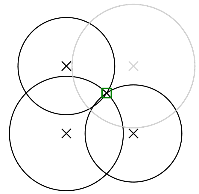
(a)

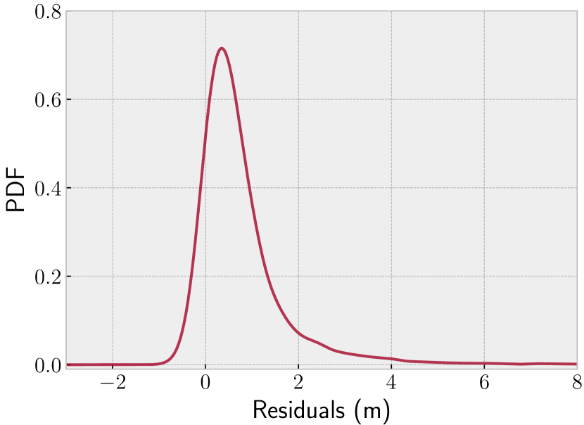
(b)

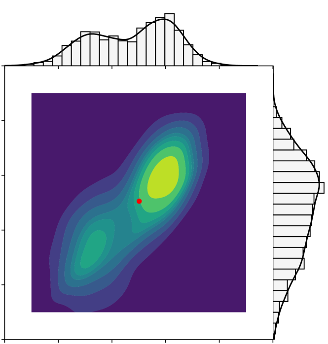
(c)

Figure 1: Problem formulation for NLOS reception in terrestrial ranging and corresponding challenges for state estimation: (a) Simulated ranging measurements (black) with 1 NLOS measurement (gray) and reference position (green); (b) Resulting right-skewed, non-gaussian ranging residuals corresponding to (a); (c) Resulting state-space multi-modalities and non-mitigated parametric estimation result (red).

The paper presents the capabilities for a tight integration of heterogeneous terrestrial measurements, including ToA, AoA and TDoA observations, with the concept of 3DMA GNSS positioning (Schwarzbach and Michler,, 2020). This is done by evolving a multi-epoch, 3DMA, grid-based Bayesian Filter, including an algorithmic generalization for the tightly coupled data fusion of the aforementioned geometric relations provided from terrestrial systems. Since the given data fusion problem formulation is reduced to a technology-independent integration of geometric relations based on spatial map data, a synergistic foundation for the future integration of opportunistic radio signals, for example including 5G-based TDoA or AoA observations or WiFi Fine Timing Measurements (FTM), is provided.

In addition to addressing the measurement model and adapting it in accordance with hybrid GNSS and terrestrial Grid Filtering (selection of sampling probabilities and their parameter settings), we also present the integration of the motion step within the grid state space representation, allowing the incorporation of vehicle dynamics within the Grid Filter. This allows the propagation of a higher entropy of the estimated state distribution within the recursive filtering structure. Furthermore, time synchronization for tightly coupled integration is discussed, as a multi-rate sequential filtering approach is presented.

In addition to conceptual work and a formal description of the approach, a real-world study in both a dynamic and a static scenario is presented in order to empirically evaluate the proposed method. Here, a local Ultra-Wideband (UWB) real-time localization system is deployed in order to augment multi-constellation GNSS pseudorange observations. The study was conducted on a testbed for automated and connected driving in an urban environment in Germany.

The rest of the paper is structured as follows: section 2 introduces the concept of the hybrid GNSS and terrestrial Grid Filter, including the discussion of potential radio technologies and respective measurement principles as well as the theory behind the hybrid Grid Filter and the integration of different geometric relations. In addition, a grid-based prediction step and a coping mechanism for multi-rate measurement synchronization is presented. The implementation of the provided theoretical background is detailed in section 3. Subsequently, section 4 presents the conducted measurement campaign, including both a static and a dynamic scenario. Based on this, a detailed evaluation of the implemented method based on the surveyed data is provided. The paper concludes with a summary and an outlook for future research work.

2 Hybrid GNSS and Terrestrial Positioning

2.1 Terrestrial Systems

Radio-based and, more generally, wireless positioning is an interdisciplinary engineering and scientific field. In the course of the years, different forms, interest groups and researchers have established themselves. However, there is no unified taxonomy for these systems in literature (Pascacio et al.,, 2021). This is due to the time difference of research and development works across different technologies. Nevertheless, it can be stated that a categorization of wireless localization systems is based on three pillars (Esposito and Ficco,, 2011; Tariq et al.,, 2017), which are presented in fig. 2.

Figure 2: Pillars of radio-based localization systems.

In unison with GNSS localization, the basis for determining location-related variables is the derivation of signal properties, more precisely properties of the signal transmission, e.g., connectivity or physical quantities of the signal. In this stage, a distinction between range-free and range-based (also referred to as geometric) can be made. This is further visualized in fig. 3, which also includes applicable measurement principles.

for tree=thick, l sep=0.3cm, s sep=0.8cm, edge=semithick, where level=0parent, where level=1 minimum height=0.2cm, child, parent anchor=south west, tier=p, l sep=0.05cm, for descendants=grandchild, minimum height=0.2cm, anchor=120, edge path= [edge] (!to tier=p.parent anchor) —-(.child anchor)edge label; , , [Measurement Principles [Range-free [Proximity [Hop-based [Received Signal Strenght (RSS) [Channel State Information (CSI) ] ] ] ] ] [Range-based [RSS [Angle of Arrival (AoA) [Phase of Arrival (PoA) [Time of Arrival (ToA) [Round-Trip Time (RTT) [Time Difference of Arrival (TDoA) ] ] ] ] ] ] ] ]

Figure 3: Classification of wireless measurement principles as a basis for position determination.

For geometry-free approaches, there is a strong (positive) correlation of the number of available infrastructure and end devices that participate in the positioning process. In general, the achievable positioning quality of these geometry-free approaches is comparatively low (Chowdhury et al.,, 2016).

Range-based approaches on the other hand, allow the geometric interpretation of derived signal quantities. Applicable radio technologies and corresponding geometric measurement principles are mapped in table 1. This allows an overview on both system candidates and the discussion of advantages of the measurement principles, e.g. hardware availability, computational complexity or achievable accuracies. Further information can be found in (Zafari et al.,, 2019; Mendoza-Silva et al.,, 2019).

Table 1: Mapping of range-based measurement principles and available technolgies for radio-based positioning.

	WiFi	BLE	ZigBee	UWB	5G
RSS	✓	✓	✓	✓	✓
AoA	✓	✓	✓	✓	✓
PoA	✗	✓	✓	✗	✓
RTT	✓	✗	✗	✓	✗
TDoA	✗	✗	✗	✓	✓

In this context, promising system candidates for hybrid GNSS terrestrial positioning for transportation and logistic applications as well as seamless indoor outdoor positioning are given by:

• WiFi-based Fine Timing Measurements (FTM) (Yu et al.,, 2020; Gentner et al.,, 2020);

• BLE-based AoA implemented from version 5.1 (Sambu and Won,, 2022) and PoA Ranging (Zand et al.,, 2019);

• 5G-based AoA and TDoA integration (Talvitie et al.,, 2019; Xhafa et al.,, 2021);

• UWB-based Two-Way Ranging or TDoA (Chiasson et al.,, 2023).

As previously stated, the presented work focuses on the hybrid integration of terrestrial systems and GNSS based on a Grid Filter implementation. Therefore, individual quantities of different origin are abstracted to their geometric primitives and integrated on this level. By this tightly-coupled approach it is possible that no system-individual position solutions have to be available for an integration and the requirements concerning the available observation quantities can be reduced. Thus, individual observations can also be used to support the position information.

2.2 Hybrid Grid Filter

The use of a grid-based representation of the state space for probabilistic filtering is fundamentally suitable for a variety of localization tasks and heterogeneous inputs Thrun et al., (2005). In general, the proposed hybrid Grid Filter follows the well-studied prediction and observation structure of a Recursive Bayes Filter (Thrun et al.,, 2005), similar to the well-known Extended Kalman Filter or the Particle Filter. In this section we will present the general framework of a multi-epoch, hybrid Grid Filter and provide background information of identified challenges for hybrid Grid Filters: Generic measurement models, state propagation for dynamic applications and time synchronization for hybrid information fusion.

The general framework in accordance with the Recursive Bayes Filter (RBF) structure is given in fig. 4. The following section will incorporate the accompanying calculation steps and their theoretical background as well as the final implementation of the method.

Figure 4: Generic RBF structure (according to Schwarzbach et al., (2020)).

2.2.1 Measurement Model

As aforementioned, the focus of the work lies on a general integration of geometric inputs, complementary to global GNSS positioning. Similar to 3DMA likelihood-based localization frameworks, e.g. (Groves et al.,, 2020) or (Ng et al.,, 2020), a translation of available measurements in a probabilistic manner needs to be performed. For simplification reasons, the following explanations concerning the implementation of the measurement models are detailed using a local two-dimensional and equidistant grid. A generalization using digital maps can easily be done by using discrete, multidimensional and globally referenced geodata, such as digital surface models (DSM) (Schwarzbach and Michler,, 2020). The basic computational steps are given in fig. 5:

Figure 5: Schematic approach to transform geometric relations into probabilistic grid-based state space.

First, the definition of a generic, discrete and finite state space according is required. The result of this initialization are $i=1,\dots,I$ grid points $\boldsymbol{\mathrm{x}}_{i}$ of arbitrary dimension. Given $n=1,\dots,N$ available reference points $\boldsymbol{{x}}^{n}F=[x^{n},y^{n},z^{n}]^{\intercal}$, the geometric relations between the defined state space $\boldsymbol{\mathrm{x}}_{i}$ and $\boldsymbol{{x}}^{n}$ are considered by calculating the innovations $\boldsymbol{\mathrm{y}}_{i}^{n}$. This is done by calculating the difference of the present observations $\boldsymbol{\mathcal{Z}}^{n}$ and the known relations between grid points and reference points $\boldsymbol{\Gamma}_{i}^{n}$:

$$\boldsymbol{\mathrm{y}}_{i}^{n}=\boldsymbol{\mathcal{Z}}^{n}-\boldsymbol{\Gamma}_{i}^{n}\;.$$ (1)

The most common relations applicable for radio-based positioning are summarized in table 2.

Table 2: Calculation of geometric relations between reference and grid points.

Geometrical relation	Calculation
Distance (ToA / RTT)	$\boldsymbol{\Gamma}_{\text{distance}}^{i,j}=\left|\left|\boldsymbol{\textrm{x}}^{n}-\boldsymbol{\textrm{x}}_{i}\right|\right|_{2}$
Hyperbolic (TDoA)	$\boldsymbol{\Gamma}_{\text{hyperbolic}}^{i,j}=\left|\left|\boldsymbol{\textrm{x}}^{n}-\boldsymbol{\textrm{x}}_{i}\right|\right|_{2}-\left|\left|\boldsymbol{\textrm{x}}^{j+1}-\boldsymbol{\textrm{x}}_{i}\right|\right|_{2}$
Angle (AoA)	$\boldsymbol{\Gamma}_{\text{angle}}^{i,j}=\arctan\frac{y^{n}-y_{i}}{x^{n}-x_{i}}$

For the innovations obtained in eq. 1 for each grid point and each observation, a likelihood, is subsequently calculated under the assumption of a statistical model. This statistical model is available in the form of a probability density function (pdf) and characterizes the expected uncertainties of the respective observations. Given a generic statistical distribution (e.g. Gaussian) $\mathcal{D}(0,\boldsymbol{\Sigma})$, we can obtain the Likelihood of each position candidate from Thrun et al., (2005):

$$\textbf{p}_{i}^{n}(\boldsymbol{\mathcal{Z}}^{n}|\boldsymbol{\textrm{x}}_{i})\leftarrow\mathcal{D}(\textbf{{y}}_{i}^{j},\boldsymbol{\Sigma})\;,$$ (2)

where $\boldsymbol{\Sigma}$ represents the scale parameter and therefore the statistical properties of the assumed pdf. In the case of Gaussian uncertainty, this represents the covariance matrix. The final combination of all observations respectively their likelihoods over all grid points is performed (here without consideration of the propagated likelihoods discussed in section 2.2.2) by means of:

$$\boldsymbol{p}_{i}=\eta\sum_{j}\textbf{p}_{i}^{n}(\boldsymbol{\mathcal{Z}}^{n}|\boldsymbol{\textrm{x}}_{i})\;,$$ (3)

where $\eta$ represents the normalization factor according to Bayes’ rule. The result of this calculation for the geometric relations given in table 2 are depicted in fig. 6. Here, the Likelihood obtained from four reference points (red) is given. The statistical model applied is a Gaussian distribution.

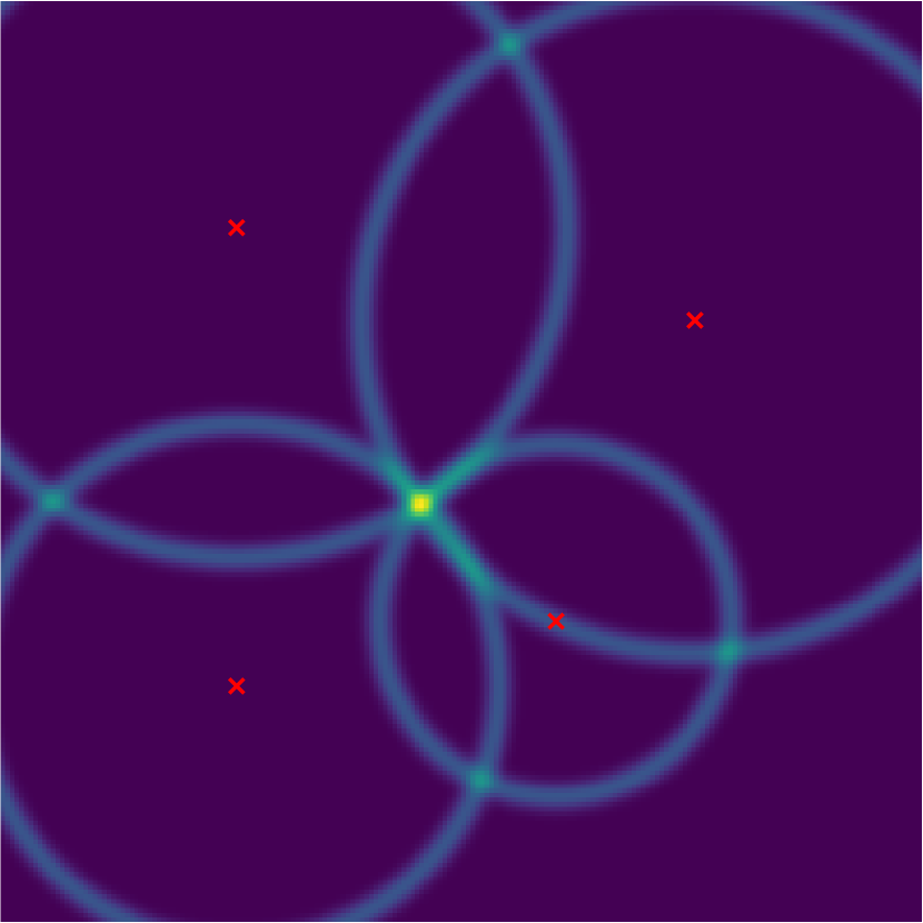
(a)

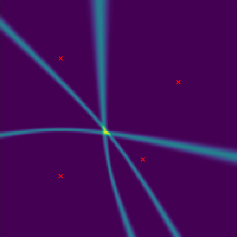
(b)

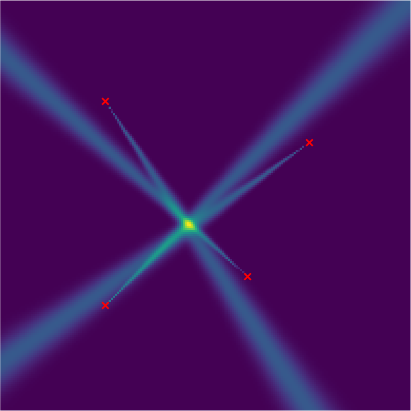
(c)

Figure 6: Likelihood representation of geometric position lines in an equidistant two-dimensional grid based on obtaining spatial relations in a radio network (anchor points red, value of Likelihood color coded): (a) Distances, (b) Hyperbolic und (c) Angle.

In addition, Grid Filtering easily allows a combination of different geometrical relations within one or consecutive measurement steps, which also enables localization systems with less required infrastructure respectively reference points. The integration of GNSS and terrestrial observations is further detailed in section 3.

2.2.2 Prediction step

An important component of dynamic state estimation respectively multi-epoch filtering is the prediction step, which takes a motion model and/or sensor information about the object motion into account. For dynamic state estimation based on the EKF approach, velocities, direction of motion, accelerations, and others are considered in the course of mathematical modeling depending on the model degree Balzer et al., (2014). For the estimation of these motion quantities, the use of EKF approaches and their derivatives has become established, since higher-dimensional state vectors can be implemented in a computationally efficient manner and these sensors satisfy the strict requirements of parametric estimation methods. This has also been applied in previous works addressing multi-epoch 3DMA filtering in (Zhong and Groves, 2022b, ).

Nevertheless, an integration of rudimentary motion information within the prediction step of the Grid Filter is possible and absolutely necessary in the context of the possible asynchronicity of observations of heterogeneous origin (cf. section 2.2.3). The approach of the grid-based computation of the prediction step is based on the determination of the translation likelihoods between the realizations (position candidates) $\boldsymbol{\mathrm{x}}_{i}$ present in the state space. For this purpose, a probability-based plausibility check of the transition from one system candidate to another is performed based on dynamics data of an object or starting from model assumptions.

The two basic quantities for characterizing the motion of an object within a grid-based state representation are the object velocity $v_{k}$ and its heading $\theta_{k}$. The representation of the motion in this form is called odometry-based information Thrun et al., (2005). The grid integration here is two-dimensional within the $x$-$y$ plane of the object to be located.

The dynamics information is processed individually within the likelihood grid and then combined. The underlying geometric relations are to be applied in analogy to the likelihood transfer of cooperative measured quantities listed in table 2. Here, a velocity measurement represents a time-scaled distance determination, where $\Delta T_{k}$ represent the temporal length of the prediction step as a function of the measurement rates and the availability of observation information. Furthermore, the heading represents an angular relation between the object orientation and a reference direction.

The peculiarity of the non-parametric estimation approach, compared to parametric estimators for dynamical systems (e.g. EKF), is that the motion prediction is performed not only for one position realization, in the case of parametric estimation this corresponds to the state vector consisting of the estimated mean values, but for all position hypotheses $\boldsymbol{\mathrm{x}}_{i}$. Thus, the motion prediction of non-parametric methods is associated with a comparatively significant increase in computational complexity. However, this also allows possibility to consider multi-modalities present in the state space. Thus, it is possible to obtain an increased information content within the state space in the prediction step compared to parametric approaches.

According to the definition of RBF, an existing velocity measurement or model assumption $v$ is also considered as a probabilistic quantity and thus represents in its simplest form an average value of the existing velocity in the direction of motion. This is further subject to an uncertainty $\sigma_{\text{v}}^{2}$, which can be parameterized empirically from available sensor data or model-based. The resulting prediction of motion is given as follows. First, for a candidate position $\boldsymbol{\mathrm{x}}_{i}$, the known distance $\boldsymbol{d}_{i,j}$ to all other candidate positions $\boldsymbol{\mathrm{x}}_{j}$ is calculated:

$$\boldsymbol{d}_{i,j}=\boldsymbol{\Gamma}_{i,j}=\left|\left|\boldsymbol{\textrm{x}}_{j}-\boldsymbol{\textrm{x}}_{i}\right|\right|_{2}\quad\text{with}\quad i\neq j\;.$$ (4)

Subsequently, the determination of the residuals $\boldsymbol{\mathrm{y}}_{i,j}^{\text{v}}$ between the determined distances $\boldsymbol{d}_{i,j}$ and the present velocity measurement $v_{k}$ in combination with the time difference $\Delta T_{k}$ is performed:

$$\boldsymbol{\mathrm{y}}_{i,j}^{\text{v}}=v_{k}\cdot\Delta T_{k}-\boldsymbol{d}_{i,j}\;.$$ (5)

Thus, concentric residuals arise, which have their origin in the used position hypothesis and whose radius corresponds to the time-scaled distance equivalent of the velocity measurement. In analogy to the calculation of the likelihood of the observations, a probabilistic sampling of the residuals based on an assumed stochastic model is performed to determine the predicted likelihood $\boldsymbol{\overline{p}}_{i,j}^{\text{v}}$, which is assumed to follow a Gaussian Distribution $\mathcal{N}(0,\sigma_{v}^{2})$ :

$$\boldsymbol{\overline{p}}_{i,j}^{\text{v}}\leftarrow\mathcal{N}(\boldsymbol{\textrm{y}}_{i,j}^{\text{h}},\sigma_{\text{v}}^{2})\;.$$ (6)

The given calculation steps are repeated for all grid points. As a final step a calculation of the total likelihood:

$$\overline{\boldsymbol{p}}_{i}^{\text{v}}=\sum_{j}\overline{\boldsymbol{p}}_{i,j}^{\text{v}}\;.$$ (7)

The integration of the heading information is done in analogy considering the measured or assumed heading $\theta_{k}$, its uncertainty $\sigma_{2}^{\text{h}}$, the residuals of the heading $\boldsymbol{\mathrm{y}}_{i,j}^{\text{h}}$ and the predicted likelihood $\overline{\boldsymbol{p}}_{i}^{\text{h}}$ by means of:

$$\boldsymbol{\alpha}_{i,j} =\arctan\frac{y_{j}-y_{i}}{x_{j}-x_{i}}\quad\text{mit}\quad i\neq j\;,$$ (8)

$$\boldsymbol{\mathrm{y}}_{i,j}^{\text{h}} =\theta_{k}-\boldsymbol{\alpha}_{i,j}\;,$$ (9)

$$\boldsymbol{\overline{p}}_{i,j}^{\text{h}} \leftarrow\mathcal{N}(\boldsymbol{\textrm{y}}_{i,j}^{\text{h}},\sigma_{\text{h}}^{2})\;,$$ (10)

$$\overline{\boldsymbol{p}}_{i}^{\text{h}} =\sum_{j}\overline{\boldsymbol{p}}_{i,j}^{\text{h}}\;.$$ (11)

Given the availability of both measurements $v_{k}$ and $\theta_{k}$, the resulting likelihood of the prediction step is obtained taking into account the normalized likelihood of the observation model (cf. eq. 3) of the last measurement epoch:

$$\overline{\boldsymbol{p}}_{i}=\sum_{i}\left(\overline{\boldsymbol{p}}_{i}^{\text{v}}\cdot\overline{\boldsymbol{p}}_{i}^{\text{h}}\right)\;\boldsymbol{p}_{i}\;.$$ (12)

A visualization of the calculation step for a candidate position within a probability grid is shown as an example in fig. 7.

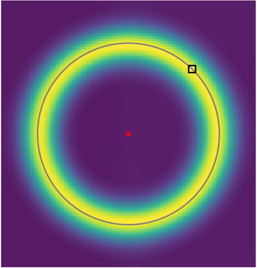
(a)

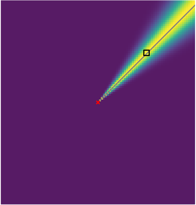
(b)

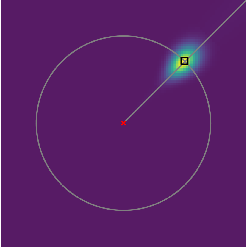
(c)

Figure 7: Visualization of the grid-based prediction step based on dynamics information or model assumptions (true values are given in grey, red indicates the position candite of interest $i$): (a) Velocity likelihood $\overline{\boldsymbol{p}}_{i}^{\text{v}}$ $v_{k}$; (b) Heading likelihood $\overline{\boldsymbol{p}}_{i}^{\text{h}}$ $\theta_{k}$; (c) Fusion according to eq. 12.

Due to the finite nature of the discrete state space representation, a system propagation for global positioning problems needs to also be accounted, as moving objects are able to leave the initially defined state space. A procedure for this task is detailed in (Zhong and Groves, 2022b, ) and therefore is not further addressed in this paper.

2.2.3 Time Synchronization

Time synchronization for hybrid positioning methods, especially with multi-rate systems has recently been addressed for GNSS and 5G Bai et al., 2022a or GNSSS and UWB in Guo et al., (2023). Thereby, a possible synchronicity respectively handling of asynchronous observations especially considering different measurement rates is imperative, as this can lead to cumulative errors in the data fusion process. This concern is further enhanced in the presence of additional terrestrial systems due to the unknown time-offset of the individual systems and unequal, potentially non-deterministic update rates.

As pointed out in (Guo et al.,, 2023) it is essential, that observations at different rates need to be processed. In (Retscher et al.,, 2023), individual measurement models for GNSS and combined GNSS/UWB are defined. However, a simultaneous processing can only be realized if the time offset between the systems is compensated, especially in dynamic scenarios. Another major challenge poses the handling of out of sequence measurements (Muntzinger et al.,, 2010). However, since we only discuss the integration of radio based inputs, the present measurement rates are comparably low. Therefore, only a timing consistency check between the time stamps of the sensor information is performed. In addition, we opt to implement a multi-rate sequential filtering approach based on the sensor time stamps of the individual sensor systems.

Essentially, the multi-rate measurements are compensated by the introduced motion model, accounting for possible pose changes of the object within a measurement update window. This procedure is schematically presented in fig. 8. Since, a grid-based motion step is implemented (cf. section 2.2.2) a high entropy about the systems state is stored within the state space. Another advantage of the given approach is that once a position fix is achieved, there is generally no limitation on the amount of available measurements to perform the described measurement step. This enables the utilization of system-individual observations at different measurement epochs, while also allowing the accounting of potential multi-modalities.

Figure 8: Schematic representation of fusion of multirate measurements as sequential data fusion based on the presented prediction step.

2.2.4 State estimation

Given the calculation of an overall Likelihood consisting of the prediction step and hybrid measurement models, the final state estimation has to be performed in order to obtain the current receiver position. This can either be achieved by performing a maximum likelihood respectively for the presented Bayesian approach a maximum a-posteriori (MAP) estimation (Bar-Shalom et al.,, 2001) or by performing a weighted mean (WM) given all samples (Minetto,, 2020). However, both approaches pose a variety of challenges for global positioning as summarized in table 3.

Table 3: Advantages and disadvantages of conventional state estimators for grid-based estimation.

	Advantages	Disadvantages
MAP	Maximum in case of multimodal distribution in state space	accuracy of estimation correlated with grid resolution and can only correspond to defined position hypotheses
	Simple, efficient implementation	Potential loss of information, since spatial realization of likelihood is not taken into account.
WM	Total information of the likelihood of the state space is considered	State space covers a large area for global positioning, therefore irrelevant areas are considered.

Therefore, similar to we apply a two-step approach for deriving the current state estimation $\hat{\boldsymbol{\mathcal{X}}}_{k}$ at time step $k$:

1. Calculation of MAP by maximizing the obtained likelihood function

2. Calculation of WM using the MAP as circle center given an user-defined radius $\mathrm{R}$ including $I_{\mathrm{R}}$ grid points.

This yields the state estimation $\hat{\boldsymbol{\mathrm{x}}}_{k}=\left[\hat{\boldsymbol{x}}_{k},\hat{\boldsymbol{y}}_{k},\hat{\boldsymbol{z}}_{k}\right]^{\intercal}$ with:

$$\hat{\boldsymbol{x}}_{k}=\frac{\sum_{i}^{I_{\mathrm{R}}}\boldsymbol{p}_{i}(x_{i}|\boldsymbol{\mathcal{Z}})\cdot\boldsymbol{{x}}_{i}}{\sum_{i}^{I_{\mathrm{R}}}\boldsymbol{p}_{i}(x_{i}|\boldsymbol{\mathcal{Z}})}\quad\hat{\boldsymbol{y}}_{k}=\frac{\sum_{i}^{I_{\mathrm{R}}}\boldsymbol{p}_{i}({y}_{i}|\boldsymbol{\mathcal{Z}})\cdot\boldsymbol{{y}}_{i}}{\sum_{i}^{I_{\mathrm{R}}}\boldsymbol{p}_{i}({y}_{i}|\boldsymbol{\mathcal{Z}})}\quad\hat{\boldsymbol{z}}_{k}=\frac{\sum_{i}^{I_{\mathrm{R}}}\boldsymbol{p}_{i}({z}_{i}|\boldsymbol{\mathcal{Z}})\cdot\boldsymbol{{z}}_{i}}{\sum_{i}^{I_{\mathrm{R}}}\boldsymbol{p}_{i}({z}_{i}|\boldsymbol{\mathcal{Z}})}\;,$$ (13)

3 Implementation

3.1 Overview

The implementation of the approach is based on the theoretical models and design considerations outlined in section 2. An overview is provided in fig. 9. The sensor components are synchronized to match a common time frame. As for GNSS, sensor data consists of satellite ephemeris data (NAV) and estimates of pseudoranges, carrier-phase, doppler and carrier-to-noise-ratio (OBS). In a preprocessing step, satellite positions are calculated and pseudoranges are corrected for error components, which can be modeled. This includes satellite clock bias and atmospheric errors as described in basic GNSS literature (Kaplan et al.,, 2005). The GNSS measurement step estimates the likelihood of each grid point based on given satellite positions and corrected pseudoranges. The measurement model is described in detail in section 3.2.1. The respective UWB measurement model relies on given anchor positions and ranging measurements for likelihood estimation. Furthermore, a motion model is incorporated, which uses heading and velocity measurements for likelihood estimation. Those measurements can be based on IMU sensor data, odometry or other sensor hardware. In case of absence of these input information, generic motion models can be applied. The resulting likelihood of each measurement step is then used to update the grid probabilities. Furthermore, each GNSS or UWB step triggers the state estimation. With this, the state vector is updated based on the current grid probability space as discussed in section 2.2.4.

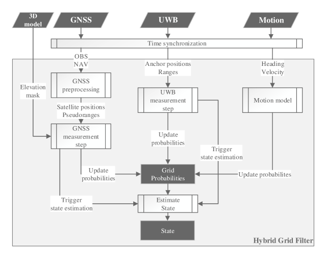
Figure 9: Flow chart of the implementation of a hybrid GNSS-UWB-motion Grid Filter.

3.2 Implementation of measurement models

The section details the implementation of the GNSS and terrestrial measurement model. Realizations of these individual Likelihoods are visualized in fig. 10. The figures are obtained from the surveyed dataset described in section 4. For both figures, the respective priors are ignored. The current state estimation based on the observation step and the corresponding reference position are also indicated.

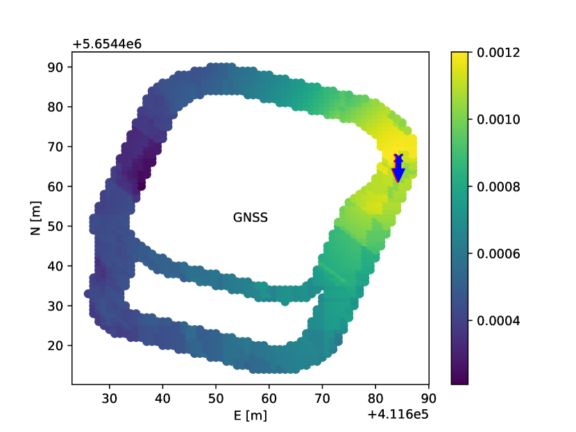
(a) GNSS

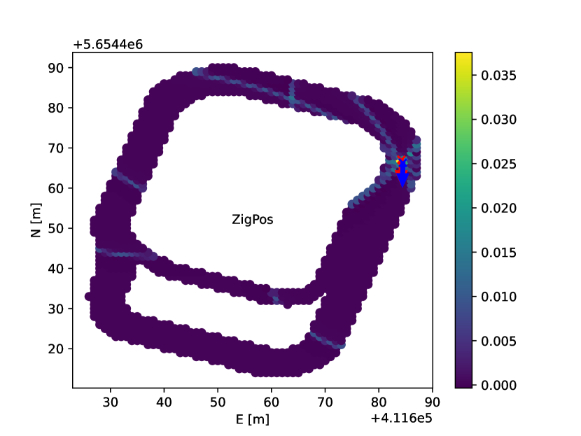
(b) Terrestrial

Figure 10: PDF after the measurement step. Reference vector (blue) and current estimate (red). Calculated Likelihoods are color coded.

3.2.1 GNSS measurement model

The presented work utilizes the well-studied Between Satellite Single Differencing (Groves and Adjrad,, 2019; Suzuki,, 2019; Schwarzbach and Michler,, 2020), suitable for code-based 3DMA positioning approaches using discrete state space representations. This is due to the removal of the receiver clock error, whose discretization is not feasible.

The generic model for a pseudorange $\rho_{r}^{s}$ is given as (Langley et al.,, 2017):

$$\rho_{r}^{s}=d_{r}^{s}+c\cdot(\delta t_{r}-\delta t^{s})+\delta_{\text{ion}}^{s}+\delta_{\text{tro}}^{s}+\varepsilon_{r}^{s}\;,$$ (14)

where $d_{r}^{s}=\left|\left|\boldsymbol{x}^{s}-\boldsymbol{x}_{r}\right|\right|_{2}=\sqrt{(x^{s}-x_{r})^{2}+(y^{s}-y_{r})^{2}+(z^{s}-z_{r})^{2}}$ represents the euclidean distance between receiver $r$ and satellite $s$ consisting of the respective Cartesian coordinates. In addition, $\delta t_{r}$ and $\delta t^{s}$ represent the receiver and the satellite clock error respectively, $\delta_{\text{ion}}^{s}$ and $\delta_{\text{tro}}^{s}$ the atmospheric error influences and finally $\varepsilon_{r}^{s}$ as the unmodeled, uncorrelated error terms for each pseudorange measurement. Following up on this, BSSD performs a differencing between respective observations. For the generic satellites $s_{1}$ and $s_{2}$ this yields:

$$\Delta\rho_{r}^{s_{1},s_{2}}=\rho_{r}^{s_{1}}-\rho_{r}^{s_{2}}.$$ (15)

Given eq. 14 we obtain:

$$\Delta\rho_{r}^{s_{1},s_{2}} =d_{r}^{s_{1}}-d_{r}^{s_{2}}+c(\delta t_{r}-\delta t_{r})-c(\delta t^{s_{1}}-\delta t^{s_{2}})+\delta_{\text{ion}}^{s_{1}}-\delta_{\text{ion}}^{s_{2}}+\delta_{\text{tro}}^{s_{1}}-\delta_{\text{tro}}^{s_{2}}+\boldsymbol{\sigma}_{r}^{s_{1},s_{2}}$$ (16)

$$=d_{r}^{s_{1}}-d_{r}^{s_{2}}+c\Delta\delta t^{s_{1},s_{2}}+\Delta\delta_{\text{ion}}^{s_{1},s_{2}}+\Delta\delta_{\text{trop}}^{s_{1},s_{2}}+\boldsymbol{\sigma}_{r}^{s_{1},s_{2}}\;.$$ (17)

The obtained model corresponds to the hyperbolic geometrical model introduced in section 2.2. Besides the elimination of the receiver-specific clock error, the observable combination mainly affects the unmodeled error terms. Due to the observation combination of BSSD and according to the error propagation with the assumption of $\sigma_{r}^{s}=\sigma_{r}^{s_{1}}=\sigma_{r}^{s_{2}}$ the influence of the stochastic error terms is given as follows (Odijk and Wanninger,, 2017):

$$\sigma_{r}^{s_{1},s_{2}}=\sigma_{\text{SD}}=\sqrt{2}\sigma_{r}^{s_{1},s_{2}}.$$ (18)

Concerning the parametrization of $\sigma_{r}^{s}$ a variety of procedures are applicable. At first, generic values according to system specifications can be set, e.g. using the GPS Signal in Space pseudorange error budget of the Standard Positioning Service Schwarzbach and Michler, (2020). Furthermore, an empirical parameter setting based on available measurements can be obtained Groves et al., (2020). For simplification, we stick to the former possibility and assume a mean-free Gaussian distribution given a line-of-sight (LOS) standard deviation of $\sigma_{r}^{s}=$7.8\text{\,}\mathrm{m}$$, leading to $\sigma_{SD}=\sqrt{2}\sigma_{r}^{s}$.

In recent literature, a variety of algorithmic 3DMA approaches with a holistic focus on adequate NLOS handling based on 3D map data are discussed, e.g. (Groves et al.,, 2020). As this not the sole focus of this work, we want to present a more general approach, which can also be implemented without the knowledge of building information or other spatial data apart from the utilized discrete state space.

BSSD approaches are implemented by selecting a pivot satellite assumed to be LOS, which is then differenced from all other observations. Depending on the estimated LOS/NLOS state of the observation, different stochastic models are applied. As presented in (Schwarzbach and Michler,, 2020), a full set differencing between all observed satellites is also applicable, resulting in a symmetric error distribution. An example given the static dataset presented in section 4 is given in fig. 13(a).

This empirical survey reveals that the differencing across all satellites produces characteristic effects:

• Case 1: The differencing of LOS measurements leads to a mean-free residual distribution.

• Case 2 and 3: Mixture densities for combined LOS/NLOS differencing depending on the associative law and if the LOS satellite is differenced from the NLOS one or vice versa. Case 2 corresponds to a positive mean, case 3 to a negative.

• Case 4: Measurement outliers, which do not fit one of the former.

In order to account for these effects, the modeling of a Gaussian mixture model (GMM) is suggested, allowing the exploitation of the full set differencing. In our case, a $3$ component GMM is applied, whose parametrization is presented in section 4. At first, a visibility prediction of observed satellites based on the building boundary information (Groves et al.,, 2020) is performed. Subsequently, full set differencing for all satellites $i$ and $j$ ($i\neq j$) is performed. The selection of the GMM component for sampling corresponds to the cases listed above:

• $i$ and $j$ are predicted as LOS satellites, $\text{GMM}_{1}$ is selected;

• $j$ is predicted LOS and $i$ is predicted NLOS, $\text{GMM}_{2}$ is selected;

• $i$ is predicted LOS and $j$ is predicted NLOS, $\text{GMM}_{3}$ is selected;

• For any other case, the differenced observations are ignored.

3.2.2 Terrestrial Measurement model

In accordance with section 2.1, a variety of technologies and accompanying measurement principles for positioning is available. The empirical validation of the method presented in section 4 introduces an UWB real-time location system based on two-way ranging, which is a realization of RTT. Respective implementations are detailed in (Sang et al.,, 2019), specified in the UWB standard and therefore available in commercial products. The underlying geometrical model corresponds to the distance measurement described in section 2.2.1.

Unlike 3DMA approaches and due to the volatile nature of the propagation between terrestrial stationary reference points and mobile devices, geometry based NLOS identification cannot be easily applied. For this task however, a variety of algorithmic mitigation strategies exist (Guvenc et al.,, 2007). The probabilistic error mitigation favored in this work uses a Likelihood mixture model, as originally presented in (Fox et al.,, 2001). The mixture Likelihood uses a set of proposal distributions to sample from and combines them using a mixture ratio $\phi$. For the example, of two proposal distributions $\mathcal{D}_{1}$ and $\mathcal{D}_{2}$ the mixture Likelihood $\mathcal{D}_{\text{ML}}$ yields:

$$\mathcal{D}_{\text{ML}}=(1-\phi)\mathcal{D}_{2}+\phi\mathcal{D}_{1}$$ (19)

The parametrization is based on a statistical analysis of UWB ranging error distributions presented in (Schwarzbach et al.,, 2021). Essentially, UWB observations and accompanying error influences $\epsilon$ are categorized into three propagation scenarios:

1. LOS reception following a mean-free Gaussian distribution,

2. NLOS reception leading to a right-skewed residual distribution or

3. Measurement outliers and failures.

The individual error magnitudes and corresponding occurrence probabilities are further discussed in section 4.

3.2.3 Motion model

The motion model is calculated as described in section 2.2.2. Basically, there are two ways of implementing the motion model. On the one hand, model-based assumptions about the motion of the object to be located can be formulated. This usually includes a model assumption of the velocity, associated with a corresponding uncertainty. On the other hand, the use of dynamic data of the object is possible. A practical implementation is the odometry motion model (Thrun et al.,, 2005), which uses the velocity of the object (speed over ground) and its heading.

The information necessary for applying the odometry motion model can be obtained from a variety of sensory inputs. In this work, we simply use the velocity and heading information estimated from the reference receiver, which is introduced in section 4. In unison with the measurement step, the (expected or assumed) quality of information for the prediction step can be modeled in a probabilistic manner (cf. eq. 4 or 12). The results of the prediction sampling step for the velocity, heading and combined information is depicted in fig. 11.

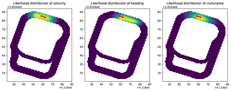
Figure 11: Motion likelihood distribution for the most probable current candidate point (red dot). Motion vector (red) is added for clarity.

4 Data Acquisition and Evaluation

4.1 Methodology

In order to evaluate the performance of the implemented approach, test runs are performed on the testbed for automated and connected driving in Dresden, Germany. Those runs consist of static and dynamic scenarios. The static test runs are conducted at fixed locations, which were geo-referenced with a survey-grade GNSS setup. The data from the static samples are used to analyze the distribution of GNSS pseudorange residuals. The parameters of the resulting multi-modal distribution are then applied in the parametrization of the final hybrid Grid Filter. This filter is evaluated in a dynamic driving test. In table 4 the conducted scenario, used sensors and reference receivers as well as the outcomes of each scenario are summarized.

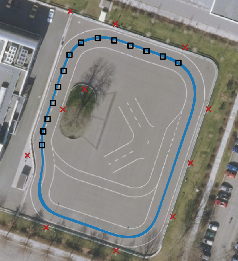
(a)

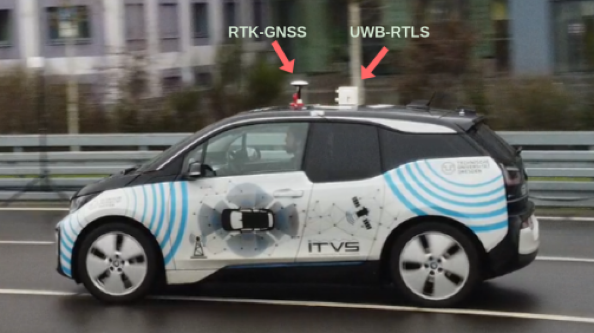
(b)

Figure 12: (a) Visualization of terrestrial pseudolites (red) and surveyed reference points: static points (black) and dynamic trajectory (blue); (b) Test vehicle with sensor setup. The antenna offset was corrected during post-processing using the known baseline between both systems.

The applied accuracy metric $\mathcal{Q}$ corresponds to the three-dimensional L2-norm $\lVert\cdot\rVert_{2}$ between the reference $\boldsymbol{\mathrm{x}}_{\text{ref},k}$ and estimated $\hat{\boldsymbol{\mathrm{x}}}_{k}$ positions at each time step $k$:

$$\mathcal{Q}=\lvert\lvert\boldsymbol{\mathrm{x}}_{\text{ref},k}-\hat{\boldsymbol{\mathrm{x}}}_{k}\rvert\lvert_{2}$$ (20)

Table 4: Test cases on testbed for automated and connected driving.

	Test case	Description	Sensors	Outcomes	Reference
I	static	14 points on testbed	u-blox F9P GNSS receiver	GNSS PR Residuals	Leica GS15
			ZigPos UWB RTLS	UWB Ranging Residuals
II	dynamic	Evaluation run	u-blox F9P GNSS receiver	Algorithmic evaluation	NovaTel PwrPak7
			ZigPos UWB RTLS

4.2 Data Set

For GNSS data collection, an u-blox F9P receiver was used on the vehicle. The recorded data include pseudorange estimates of GPS L1, Galileo E1 and Glonass L1 FDMA. As terrestrial radio system, a UWB system by Zigpos GmbH was used, which features two-way ranging based on DecaWave chip sets. For this purpose, 11 UWB anchors were placed and geo-referenced in order to be integrated with GNSS. To enable a comprehensive performance and error analysis, all measurements were referenced. The offset between UWB and GNSS antenna is corrected using the known baseline parameters between both. The static scenario consists of 4038 measurement epochs on 14 points on the testbed (cf, fig. 12). The aim is to analyze error distributions of the applied sensor systems given operation environment. For the static scenarios, a survey-grade Leica GS15 with VRS RTK correction data was used as reference receiver.

The dynamic scenario consists of a test run using a test vehicle depicted in fig. 12. The data set consists of 2066 raw measurement epochs, of which 1411 include GNSS and 655 include UWB data. The UWB measurement rate was set comparatively low to showcase the influence of terrestrial augmentation for GNSS. The reference was recorded using a Novatel PwrPak 7 with VRS RTK corrections.

4.3 Evaluation

At first, the static scenario and more specifically the quality of the available sensor information are evaluated. For this purpose, fig. 13 includes a histogram of the full set differencing approach in fig. 13(a) and the UWB ranging residuals in fig. 13(b).

As aforementioned, the full set satellite differencing yields a symmetric residual distribution. As described in section 3.2.1, the resulting mixture distribution can be approximated as GMM using a variable amount of $C$ Gaussian components associated with different weights $\omega_{c}$, means $\mu_{c}$ and variances $\Sigma_{c}$:

$$P\sim\sum_{c}^{C}w_{c}\cdot\mathcal{N}(\mu_{c},\Sigma_{c})$$ (21)

For the surveyed data, the underlying GMM is estimated using the Python library scikit-learn (Pedregosa et al.,, 2011) assuming $C=4$ components. The respective values for the BSSD GMM components are summarized in table 5. The estimated standard deviations of each sensor system is then applied in the parametrization of the measurement update step of the respective sensor.

Table 5: Estimated GMM parameter for the BSSD residuals obtained from the static scenario.

	$\omega_{c}$	$\mu_{c}$	$\Sigma_{c}$
$1$	$0.42$	$0.25$	$13.06$
$2$	$0.24$	$13.09$	$20.37$
$3$	$0.24$	$-12.61$	$21.05$
$4$	$0.01$	$-0.3$	$142.89$

In addition, the accuracy of the UWB ranging measurements is evaluated as shown in fig. 13(b). Unlike the theoretical assumptions formulated in section 3.2.2, the data does not contain any NLOS measurements, therefore this part of the mixture can be neglected. This effect can be reasoned due to the advantageous propagation conditions on the testbed. Apart from vegetation, LOS propagation is present. The parameters of the normal distribution shown in fig. 13(b) are:

$$\varepsilon_{\text{UWB}}\sim\mathcal{N}(\mu_{{UWB}},\sigma_{\text{UWB}}^{2})\quad\quad\text{with}\quad\quad\mu_{\text{UWB}}=$0.05\text{\,}\mathrm{m}$\quad\text{and}\quad\sigma_{\text{UWB}}=$0.31\text{\,}\mathrm{m}$\;.\vspace{0.5cm}$$ (22)

In addition, a variety of measurement outliers occurred, accumulating to a total of approximately $10\text{\,}\mathrm{\char 37\relax}$. Therefore, mixture ratio for the mixture Likelihood distribution can empirically be set to $\phi=0.9$.

Applying the presented hybrid Grid Filter with these parameter settings for GNSS and UWB observations to the surveyed data yields the qualitative positioning results shown in fig. 13(c). As summarized in table 6 a mean $\bar{\mathcal{Q}}=$0.64\text{\,}\mathrm{m}$$ respectively a median $\tilde{\mathcal{Q}}=$0.62\text{\,}\mathrm{m}$$ positioning error is achieved.

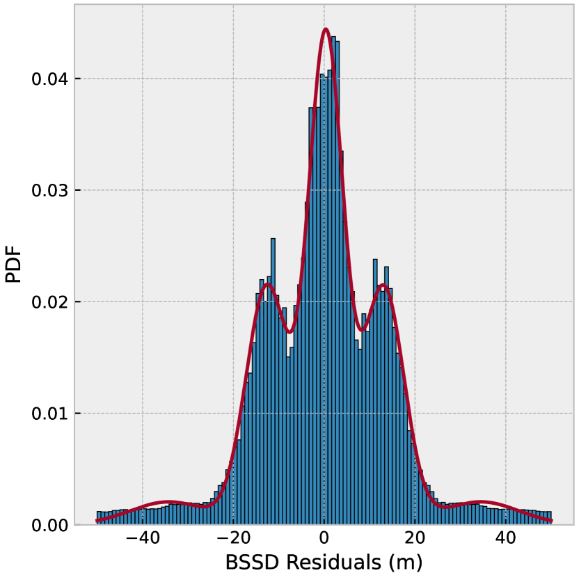
(a)

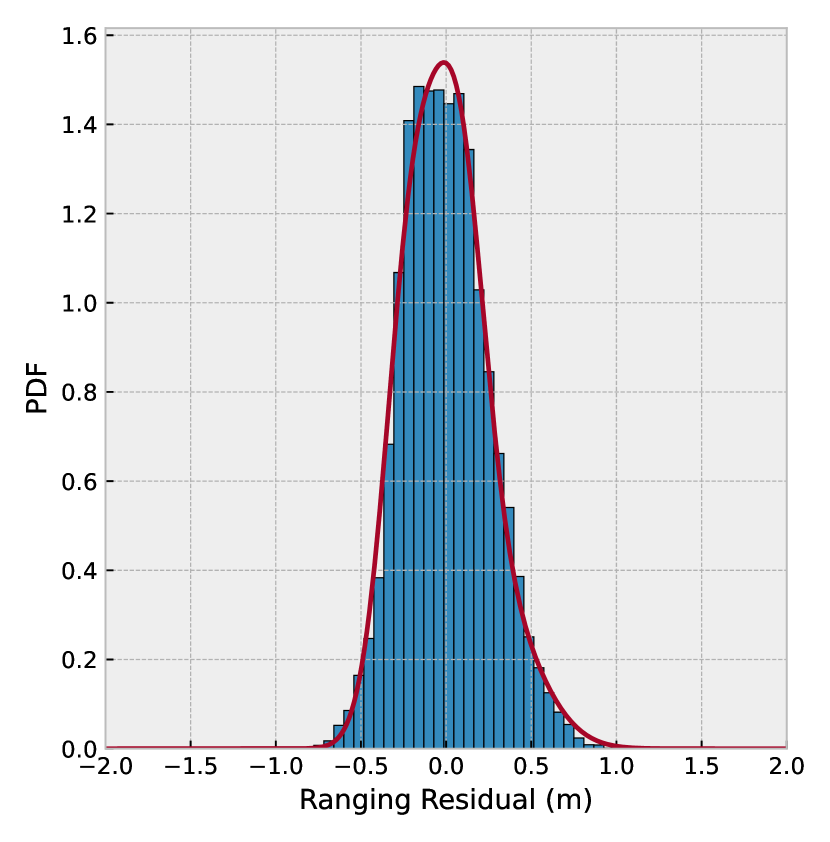
(b)

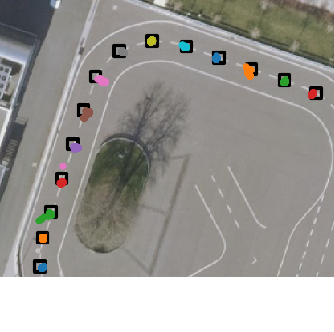
(c)

Figure 13: Histogram (blue) of the error distributions of the underlying sensor information: (a) Clock corrected GNSS pseudorange residuals and (b) UWB ranging residuals (kernel density estimation is given in red). (c) Orthofoto of qualitative positioning results for the static scenario.

A summary of descriptive statistics for the error distributions for the static and dynamic scenario is given in table 6. This includes the average error $\bar{\mathcal{Q}}$ (root mean square error), the median error $\tilde{\mathcal{Q}}$ and the error variance $\sigma_{\mathcal{Q}}^{2}$. In addition, the $\sigma$ quantiles and the $25,50,75$ percentiles of the error distributions are given.

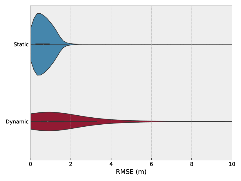
(a)

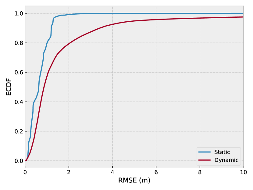
(b)

Figure 14: Statistical evaluation of the root squared error for both the static (blue) and dynamic (red) scenario: a) Violinplot and b) empirical cumulative density function (ECDF).

Furthermore, the proposed method and parameter settings are also applied to the dynamic data set. A quantitative error analysis for both scenarios is given fig. 14. In general, the hybrid Grid Filter applied to the dynamic scenario achieves less positioning accuracy, accumulating a mean $\bar{\mathcal{Q}}=$1.62\text{\,}\mathrm{m}$$ respectively a median $\tilde{\mathcal{Q}}=$0.84\text{\,}\mathrm{m}$$ positioning error associated with a higher error variance. This can be accounted to the fact, that the static case allows for a convergence on the correct position over a longer period of time due to the static motion model. The sequential motion update does not induce as much noise due to the constant position behavior of the system. This is further reflected in the comparably low variance of the positioning error with $\sigma_{\mathcal{Q}}^{2}=$0.21\text{\,}\mathrm{m}$^{2}$. Apart from a single outlier, observable in fig. 13(c) (pink), which rapidly converges, the position results are comparably stable.

In contrast, the dynamic motion model allows for a smoothing of the trajectory, but does not always prevent jumps in the state space due to observation outliers. One approach to compensate for this would be a more restrictive parametrization of the motion model. However, a more loosely configured motion model facilitates recovery of biased measurements over multiple epochs. This dichotomy can be resolved by adaptive parametrization based on statistic evaluation of measurement residuals, as provided by integrity monitoring techniques such as in (Zhong and Groves, 2022a, ).

Table 6: Quantitative evaluation of the static and dynamic scenario.

Measure	$\bar{\mathcal{Q}}$	$\tilde{\mathcal{Q}}$	$\sigma_{\mathcal{Q}}^{2}$	Quantile $[$\text{\,}\mathrm{m}$]$			Percentile $[$\text{\,}\mathrm{m}$]$
	$[$\text{\,}\mathrm{m}$]$	$[$\text{\,}\mathrm{m}$]$	$[$\text{\,}\mathrm{m}$]^{2}$	$\sigma$	$2\sigma$	$3\sigma$	$25$	$50$	$75$
Static	$0.64$	$0.62$	$0.21$	$0.82$	$1.28$	$1.72$	$0.28$	$0.62$	$0.91$
Dynamic	$1.62$	$0.84$	$6.56$	$1.31$	$4.82$	$15.60$	$0.54$	$0.86$	$1.64$

5 Conclusion

In conclusion, we identify great potential in the unified integration of both GNSS observations and radio-based terrestrial relations using a hybrid Grid Filter. This is exemplified by a test run on an automotive test bed, in which GNSS, UWB and motion data are fused using an implementation of such a filter. The parametrization of the measurement model is done by applying the measurement residuals extracted from a static test, which was conducted within the same reception environment. Furthermore, 3D models are applied to account for NLOS reception. Our test shows the general feasibility of the approach, resulting in a RMSE of $1.62\text{\,}\mathrm{m}$ in the surveyed dynamic case. The results however also indicate a lot of potential for future work, including:

• Inclusion of additional sensor systems

• Application of additional geometric relations, e.g. terrestrial AoA or TDoA

• Fine-tuning of measurement models, integrated adaption of advanced 3DMA approaches as well as outlier detection for both GNSS and terrestrial observations

In addition to these algorithmic potentials, we also recognize different application potentials to further evaluate the presented method, e.g. by focusing on indoor-outdoor localization scenarios or possible technology hand-over scenarios. Additionally, a data fusion with opportunistic signals within intelligent transportation systems can be addressed.

References

- (1) Bai, L., Sun, C., Dempster, A. G., Zhao, H., Cheong, J. W., and Feng, W. (2022a). GNSS-5g hybrid positioning based on multi-rate measurements fusion and proactive measurement uncertainty prediction. IEEE Transactions on Instrumentation and Measurement, 71:1–15.
- (2) Bai, Y. B., Holden, L., Kealy, A., Zaminpardaz, S., and Choy, S. (2022b). A hybrid indoor/outdoor detection approach for smartphone-based seamless positioning. Journal of Navigation, pages 1–20.
- Balzer et al., (2014) Balzer, P., Trautmann, T., and Michler, O. (2014). Epe and speed adaptive extended kalman filter for vehicle position and attitude estimation with low cost gnss and imu sensors. 2014 11th International Conference on Informatics in Control, Automation and Robotics (ICINCO), 01:649–656.
- Bar-Shalom et al., (2001) Bar-Shalom, Y., Li, X., and Kirubarajan, T. (2001). Estimation with applications to tracking and navigation: Theory algorithms and software.
- Calatrava et al., (2023) Calatrava, H., Medina, D., and Closas, P. (2023). Massive differencing of GNSS pseudorange measurements. In 2023 IEEE/ION Position, Location and Navigation Symposium (PLANS). IEEE.
- Chiasson et al., (2023) Chiasson, D., Lin, Y., Kok, M., and Shull, P. B. (2023). Asynchronous hyperbolic UWB source-localization and self-localization for indoor tracking and navigation. IEEE Internet of Things Journal, 10(13):11655–11668.
- Chowdhury et al., (2016) Chowdhury, T. J., Elkin, C., Devabhaktuni, V., Rawat, D. B., and Oluoch, J. (2016). Advances on localization techniques for wireless sensor networks: A survey. Computer Networks, 110:284–305.
- Egea-Roca et al., (2022) Egea-Roca, D., Arizabaleta-Diez, M., Pany, T., Antreich, F., Lopez-Salcedo, J. A., Paonni, M., and Seco-Granados, G. (2022). GNSS user technology: State-of-the-art and future trends. IEEE Access, 10:39939–39968.
- Esposito and Ficco, (2011) Esposito, C. and Ficco, M. (2011). Deployment of RSS-based indoor positioning systems. International Journal of Wireless Information Networks, 18(4):224–242.
- European Union Agency for the Space Programme, (2020) European Union Agency for the Space Programme (2020). Report on location-based services user needs and requirements.
- Fox et al., (2001) Fox, D., Thrun, S., Burgard, W., and Dellaert, F. (2001). Particle filters for mobile robot localization. In Sequential Monte Carlo Methods in Practice, pages 401–428. Springer New York.
- Gentner et al., (2020) Gentner, C., Ulmschneider, M., Kuehner, I., and Dammann, A. (2020). WiFi-RTT indoor positioning. In 2020 IEEE/ION Position, Location and Navigation Symposium (PLANS). IEEE.
- Grejner-Brzezinska et al., (2016) Grejner-Brzezinska, D. A., Toth, C. K., Moore, T., Raquet, J. F., Miller, M. M., and Kealy, A. (2016). Multisensor navigation systems: A remedy for GNSS vulnerabilities? Proceedings of the IEEE, 104(6):1339–1353.
- Groves and Adjrad, (2019) Groves, P. D. and Adjrad, M. (2019). Performance assessment of 3d-mapping–aided GNSS part 1: Algorithms, user equipment, and review. 66(2):341–362.
- Groves et al., (2020) Groves, P. D., Zhong, Q., Faragher, R., and Esteves, P. (2020). Combining inertially-aided extended coherent integration (supercorrelation) with 3d-mapping-aided GNSS. In Proceedings of the 33rd International Technical Meeting of the Satellite Division of The Institute of Navigation (ION GNSS+ 2020). Institute of Navigation.
- Guo et al., (2023) Guo, Y., Vouch, O., Zocca, S., Minetto, A., and Dovis, F. (2023). Enhanced EKF-based time calibration for GNSS/UWB tight integration. IEEE Sensors Journal, 23(1):552–566.
- Guvenc et al., (2007) Guvenc, I., Chong, C.-C., and Watanabe, F. (2007). NLOS identification and mitigation for UWB localization systems. In 2007 IEEE Wireless Communications and Networking Conference. IEEE.
- Huang et al., (2016) Huang, B., Yao, Z., Cui, X., and Lu, M. (2016). Dilution of precision analysis for GNSS collaborative positioning. 65(5):3401–3415.
- Huang et al., (2022) Huang, Z., Jin, S., Su, K., and Tang, X. (2022). Multi-GNSS precise point positioning with UWB tightly coupled integration. Sensors, 22(6):2232.
- Julier and Uhlmann, (2004) Julier, S. J. and Uhlmann, J. K. (2004). Unscented filtering and nonlinear estimation. Proc. IEEE Inst. Electr. Electron. Eng., 92(3):401–422.
- Kaplan et al., (2005) Kaplan, D., Elliott, and Hegarty, C. (2005). Understanding GPS: Principles And Applications.
- Langley et al., (2017) Langley, R. B., Teunissen, P. J., and Montenbruck, O. (2017). Introduction to GNSS. In Springer Handbook of Global Navigation Satellite Systems, pages 3–23. Springer International Publishing.
- Medina et al., (2020) Medina, D., Grundhofer, L., and Hehenkamp, N. (2020). Evaluation of estimators for hybrid GNSS-terrestrial localization in collaborative networks. In 2020 IEEE 23rd International Conference on Intelligent Transportation Systems (ITSC). IEEE.
- Mendoza-Silva et al., (2019) Mendoza-Silva, G. M., Torres-Sospedra, J., and Huerta, J. (2019). A meta-review of indoor positioning systems. Sensors, 19(20):4507.
- Minetto, (2020) Minetto, A. (2020). GNSS-only Collaborative Positioning Methods for Networked Receivers. PhD thesis.
- Minetto et al., (2022) Minetto, A., Bello, M. C., and Dovis, F. (2022). DGNSS cooperative positioning in mobile smart devices: A proof of concept. IEEE Transactions on Vehicular Technology, 71(4):3480–3494.
- Muntzinger et al., (2010) Muntzinger, M. M., Aeberhard, M., Zuther, S., Mahlisch, M., Schmid, M., Dickmann, J., and Dietmayer, K. (2010). Reliable automotive pre-crash system with out-of-sequence measurement processing. In 2010 IEEE Intelligent Vehicles Symposium. IEEE.
- Ng et al., (2020) Ng, H.-F., Zhang, G., and Hsu, L.-T. (2020). A computation effective range-based 3d mapping aided GNSS with NLOS correction method. Journal of Navigation, 73(6):1202–1222.
- Odijk and Wanninger, (2017) Odijk, D. and Wanninger, L. (2017). Differential positioning. In Springer Handbook of Global Navigation Satellite Systems, pages 753–780. Springer International Publishing.
- Pascacio et al., (2021) Pascacio, P., Casteleyn, S., Torres-Sospedra, J., Lohan, E. S., and Nurmi, J. (2021). Collaborative indoor positioning systems: A systematic review. Sensors, 21(3):1002.
- Pedregosa et al., (2011) Pedregosa, F., Varoquaux, G., Gramfort, A., Michel, V., Thirion, B., Grisel, O., Blondel, M., Prettenhofer, P., Weiss, R., Dubourg, V., Vanderplas, J., Passos, A., Cournapeau, D., Brucher, M., Perrot, M., and Duchesnay, E. (2011). Scikit-learn: Machine learning in Python. Journal of Machine Learning Research, 12:2825–2830.
- Raviglione et al., (2022) Raviglione, F., Zocca, S., Minetto, A., Malinverno, M., Casetti, C., Chiasserini, C., and Dovis, F. (2022). From collaborative awareness to collaborative information enhancement in vehicular networks. Vehicular Communications, 36:100497.
- Retscher et al., (2023) Retscher, G., Kiss, D., and Gabela, J. (2023). Fusion of GNSS pseudoranges with UWB ranges based on clustering and weighted least squares. Sensors, 23(6):3303.
- Sambu and Won, (2022) Sambu, P. and Won, M. (2022). An experimental study on direction finding of bluetooth 5.1: Indoor vs outdoor. In 2022 IEEE Wireless Communications and Networking Conference (WCNC). IEEE.
- Sang et al., (2019) Sang, C. L., Adams, M., Hörmann, T., Hesse, M., Porrmann, M., and Rückert, U. (2019). Numerical and experimental evaluation of error estimation for two-way ranging methods. Sensors, 19(3):616.
- Schwarzbach et al., (2020) Schwarzbach, P., Michler, A., and Michler, O. (2020). Tight integration of GNSS and WSN ranging based on spatial map data enhancing localization in urban environments. In 2020 International Conference on Localization and GNSS (ICL-GNSS). IEEE.
- Schwarzbach and Michler, (2020) Schwarzbach, P. and Michler, O. (2020). GNSS probabilistic single differencing for non-parametric state estimation based on spatial map data. In 2020 European Navigation Conference (ENC). IEEE.
- Schwarzbach et al., (2021) Schwarzbach, P., Weber, R., and Michler, O. (2021). Statistical evaluation and synthetic generation of ultra-wideband distance measurements for indoor positioning systems. pages 1–1.
- Suzuki, (2019) Suzuki, T. (2019). Mobile robot localization with GNSS multipath detection using pseudorange residuals. Advanced Robotics, 33(12):602–613.
- Talvitie et al., (2019) Talvitie, J., Levanen, T., Koivisto, M., and Valkama, M. (2019). Positioning and tracking of high-speed trains with non-linear state model for 5g and beyond systems. In 2019 16th International Symposium on Wireless Communication Systems (ISWCS). IEEE.
- Tariq et al., (2017) Tariq, Z. B., Cheema, D. M., Kamran, M. Z., and Naqvi, I. H. (2017). Non-GPS positioning systems. ACM Computing Surveys, 50(4):1–34.
- Thrun et al., (2005) Thrun, S., Burgard, W., and Fox, D. (2005). Probabilistic Robotics (Intelligent Robotics and Autonomous Agents). The MIT Press.
- Xhafa et al., (2021) Xhafa, A., del Peral-Rosado, J. A., López-Salcedo, J. A., and Seco-Granados, G. (2021). Evaluation of 5g positioning performance based on UTDoA, AoA and base-station selective exclusion. Sensors, 22(1):101.
- Yan et al., (2022) Yan, Y., Bajaj, I., Rabiee, R., and Tay, W. P. (2022). A tightly coupled integration approach for cooperative positioning enhancement in DSRC vehicular networks. IEEE Transactions on Intelligent Transportation Systems, pages 1–17.
- Yu et al., (2020) Yu, Y., Chen, R., Liu, Z., Guo, G., Ye, F., and Chen, L. (2020). Wi-fi fine time measurement: Data analysis and processing for indoor localisation. Journal of Navigation, 73(5):1106–1128.
- Zafari et al., (2019) Zafari, F., Gkelias, A., and Leung, K. K. (2019). A survey of indoor localization systems and technologies. 21(3):2568–2599.
- Zand et al., (2019) Zand, P., Romme, J., Govers, J., Pasveer, F., and Dolmans, G. (2019). A high-accuracy phase-based ranging solution with bluetooth low energy (BLE). In 2019 IEEE Wireless Communications and Networking Conference (WCNC). IEEE.
- (48) Zhang, G., Icking, L., Hsu, L.-T., and Schön, S. (2021a). A study on multipath spatial correlation for GNSS collaborative positioning. In Proceedings of the 34th International Technical Meeting of the Satellite Division of The Institute of Navigation (ION GNSS+ 2021). Institute of Navigation.
- (49) Zhang, G., Ng, H.-F., Wen, W., and Hsu, L.-T. (2021b). 3d mapping database aided GNSS based collaborative positioning using factor graph optimization. IEEE Transactions on Intelligent Transportation Systems, 22(10):6175–6187.
- (50) Zhong, Q. and Groves, P. (2022a). Outlier detection for 3d-mapping-aided GNSS positioning. In ION GNSS+, The International Technical Meeting of the Satellite Division of The Institute of Navigation. Institute of Navigation.
- (51) Zhong, Q. and Groves, P. D. (2022b). Multi-epoch 3d-mapping-aided positioning using bayesian filtering techniques. NAVIGATION: Journal of the Institute of Navigation, 69(2):navi.515.