Forecasted Treatment Effects

Abstract

We consider estimation and inference of the effects of a policy in the absence of a control group. We obtain unbiased estimators of individual (heterogeneous) treatment effects and a consistent and asymptotically normal estimator of the average treatment effect. Our estimator averages over unbiased forecasts of individual counterfactuals, based on a (short) time series of pre-treatment data. The paper emphasizes the importance of focusing on forecast unbiasedness rather than accuracy when the end goal is estimation of average treatment effects. We show that simple basis function regressions ensure forecast unbiasedness for a broad class of data-generating processes for the counterfactuals, even in short panels. In contrast, model-based forecasting requires stronger assumptions and is prone to misspecification and estimation bias. We show that our method can replicate the findings of some previous empirical studies, but without using a control group.

Keywords: Polynomial regressions; Forecast unbiasedness; Counterfactuals; Misspecification; Heterogeneous treatment effects

1 Introduction

Evaluating policies, or treatments, is a central task in causal inference. Such evaluations usually require the construction of counterfactuals, i.e., outcomes that the treated would have experienced had they not received the treatment. When evaluating policies with partial participation, the convention is to construct counterfactuals for the treated using observed data on the control, i.e. on those who do not receive the treatment and who are observed at every time period as the treated. When there is universal participation, researchers in economics typically rely on structural models for policy evaluation.

In this paper, we introduce an alternative approach for the evaluation of policies with universal participation. While our approach does not rely on structural models, it is unique in its focus on understanding what assumptions on the data-generating process (DGP) for the counterfactuals are needed to consistently estimate the effect of a universal treatment. With partial participation, the literature has not conventionally discussed the DGP, opting instead for high-level assumptions such as unconfoundedness or parallel paths. Recent literature has illustrated the types of assumptions implicitly imposed on individual dynamic choice by these high-level assumptions (e.g., Ghanem et al. (2022); Marx et al. (2023)), and our approach can be seen as reflecting a possibly growing interest in making assumptions on the DGP explicit.

Our parameter of interest is the average treatment effect on the treated (ATT). Our baseline method uses individual time series of pre-treatment outcomes to forecast individual counterfactuals. The time series can be short. The cross-sectional average of individual treatment effects, i.e. the individual differences between the observed post-treatment outcome at a particular time and the forecasted counterfactual, is taken as an estimate of the ATT at that time period. We call our estimator Forecasted Average Treatment effect (FAT). We show that, even in short panels, FAT is a consistent and asymptotically normal estimator of the ATT under two high-level assumptions: (1) the forecasts are unbiased on average, and (2) the average differences between the observed post-treated outcomes and the forecasted counterfactuals satisfy a central limit theorem. The main contribution of this paper is to characterize both the class of DGPs for the individual counterfactuals and the forecast methods that satisfy these requirements.

Focusing on individual-level forecasts allows for heterogeneous treatment effects, unbalanced panels, and staggered (or individual-specific) treatment timing. On the other hand, achieving robustness to the absence of a valid control group naturally comes at a cost: Our baseline method rules out unforecastable common shocks that affect all treated individuals between the time of implementation and evaluation of the treatment. In the presence of unforecastable common shocks, recovering the ATT requires access to a (control) group that is subject to the shock but not to the treatment, see Section C.2 in the Online Appendix. This illustrates the trade-offs involved in recovering the ATT: Assumptions must be placed on either a control group if available, or on the counterfactuals of the treated group. A key insight of this paper is that, surprisingly, the assumptions on the counterfactuals of the treated group do not include correct model specification. All that is needed are forecasts of the counterfactuals that are unbiased on average across individuals.

Forecast unbiasedness is typically not the main concern in time series and panel forecasting, which focuses instead on accuracy (i.e., variance reduction at the cost of some bias). Our first contribution is to show that forecasts based on basis function regressions, i.e. forecasts based on regressing individual pre-treatment outcomes on known basis functions of time (such as polynomial time trends), deliver unbiased estimators of the individual treatment effects, and that FAT based on these forecasts is a consistent and asymptotically normal estimator of the ATT. Our second contribution is to show that forecast unbiasedness holds for a large class of DGPs that expresses the counterfactuals as, potentially, the sum of two individual-specific unobserved components: a mean-stationary process and a random walk. Importantly, this is a large and flexible class that encompasses, e.g., linear panel models with fixed effects, lagged outcomes with heterogeneous autoregressive parameters, and stochastic trends. If the DGP includes a deterministic trend, an additional requirement is imposed. The additional requirement is that the basis functions used to produce the forecast must be correctly specified. This result emphasizes that it is not necessary to model the stochastic component of the counterfactuals to obtain unbiased forecasts. Rather, the focus should be on correctly specifying the deterministic trend component (up to its order), if this component is believed to be present.

A useful way to check the validity of the assumptions on the DGP is to consider placebo FAT estimates, obtained by pretending that the treatment was implemented before its actual implementation, and computing the corresponding placebo FAT. Placebo estimates that are statistically close to zero indicate that there is not enough evidence to reject the assumptions on the counterfactuals required by our method, and give reassurance that FAT estimates the causal effect of the treatment (e.g., Arkhangelsky and Imbens (2023)).

Basis function regressions are easy to implement. Letting $i$ index an individual, the order of the basis function, $q_{i}$, and the length of the estimation window, $R_{i}$, are tuning parameters that must be chosen for each individual. If feasible, plotting the individual time series of pre-treatment data can guide this choice. If the panel is balanced (and the same basis function is used across individuals), one can simply plot the time series of pre-treatment outcomes averaged across individuals. If there are trends, one can decide if they are plausibly stochastic or deterministic. In the former case, any $q_{i}$ is valid, see Theorem 1. In the latter case, our result in Theorem 2 requires that $q_{i}$ be greater than or equal to the true order. A lower $q_{i}$ delivers smaller standard errors for FAT, while a higher $q_{i}$ could guard against nonstationary initial conditions (as we show in a simulation), which are otherwise ruled out by our class of DGPs. In practice, one could report results for a small range of values for $q_{i}$. The choice of estimation window $R_{i}$ depends on balancing a desire for small standard errors (larger $R_{i}$) with concerns about possible structural instability pre-treatment (smaller $R_{i}$). For example, assuming the same choice of tuning parameters across individuals, one can report FAT based on $q\in\{0,1,2\}$ if there are no obvious trends in averaged pre-treatment data and using a small $R$ (the smallest being $R=q+1$) if there are concerns about structural instability. Otherwise $R$ is all available pre-treatment data.

The basis function regression approach only uses pre-treatment outcomes as data and does not require specifying a model. We show that covariates, including lagged outcomes, can be incorporated in the estimation of FAT by specifying a model for the counterfactuals and using it to forecast the counterfactuals. We call this approach model-based FAT. This approach requires stronger assumptions, including: correct specification of the model; availability of a consistent estimator for the coefficients if these coefficients are homogeneous; symmetry of the error term if the coefficients are heterogeneous and the covariates are lagged outcomes. Under these additional assumptions, the model-based FAT is biased, but it is still consistent and asymptotically normal. A simulation illustrates how the model-based FAT is, however, sensitive to misspecification as well as estimation bias under correct specification in small samples. Estimation bias could, in principle, be corrected, but this requires strong assumptions on the DGP and, unlike the basis function approach, rules out unit roots. This suggests that the basis function approach has desirable robustness properties, particularly in small samples. Importantly, the basis function approach bypasses the incidental parameter problem in short panels.

The paper is related to several literatures. A growing body of work uses Bayesian or machine learning methods for forecasting counterfactuals from pre-treatment data of the treated (e.g., Brodersen et al. (2015); Chernozhukov et al. (2021); Menchetti et al. (2023); Cerqua et al. (2023)), while interrupted time series analysis (e.g., Bernal et al. (2017)) and “event studies” in finance (e.g., Brown and Warner (1985)) use a special case of the approach here to forecast counterfactuals. This work focuses on forecast accuracy and, typically, leverages the availability of both long time series and consensus about the plausible DGP for the counterfactuals. In contrast, we show that a long pre-treatment time series is not necessary for consistent estimation of the ATT. In fact, our approach is well-suited for short panels. We emphasize that a sufficient condition for consistent estimation of the ATT is forecast unbiasedness and show that basis function regressions are a robust method for obtaining unbiased forecasts under weak assumptions on the class of DGPs. Model-based approaches, instead, require stronger assumptions and can suffer from misspecification and/or estimation biases that translate into poor finite sample performance.

Forecast unbiasedness has been studied in the context of time series models (Fuller and Hasza (1980); Dufour (1984)), while with a short panel, the MLE-based method in Mavroeidis et al. (2015) could be used to produce average unbiased forecasts. Key assumptions in this work are a symmetry restriction on the model errors and stationarity. In this paper, we obtain unbiased forecasts for a more general class, including stationary and nonstationary processes with heterogeneous parameters. To the best of our knowledge, the issue of unbiased forecasts with a short panel and parameter heterogeneity has not been considered for non-stationary processes.

Our analysis allows for heterogeneous treatment effects. It is well known that in this case Ordinary Least Squares or Two Way Fixed Effects estimators in linear panel data models are generally inconsistent for the average treatment effect. Proposed solutions assume the existence of a control group in every period. In addition, in order to avoid the incidental parameter problem, this literature assumes static panel models, i.e. the absence of lagged outcomes when the panel is short and the model allows for fixed effects, e.g., Angrist and Pischke (2009). Instead, our approach delivers a consistent estimator of the ATT in the absence of a control group and our class of DGPs allows for fixed effects, lagged outcomes, and time trends with fully heterogeneous parameters even when the panel is short.

Least-squares estimates of treatment effects are often interpreted as consistent estimates of certain weighted average effects to allow for the possibility of model misspecification, e.g., Theorem 1 in Chernozhukov et al. (2013). One generally has no control over the weights, which can become negative in panel data models with fixed effects. In addition, the weighted average interpretation does not address the incidental parameter problem, which occurs even for correctly specified models with homogeneous treatment effects. In contrast, our results show that, if treatment effects are estimated via averages over unbiased forecasts of counterfactuals, the correct unweighted treatment effect is consistently estimated, as long as the average is over a sufficiently large cross-section of observations. Our method thus signals a shift in focus: rather than trying to obtain consistent estimates of the model’s parameters, we focus on unbiased forecasts of counterfactuals. In this way, we avoid both the incidental parameter problem and the negative weighting issue mentioned above.

The paper is organized as follows: Section 2 presents the baseline method and Section 3 shows how to incorporate covariates. The finite sample performance of both methods is investigated in Section 4. We showcase the replication of an existing application without utilizing a control group in Section 5. Appendix A contains proofs and Appendix B discusses how to estimate the variance of our proposed estimator. An Online Appendix discusses extensions, including the existence of a control group, additional simulations and replications.

2 Baseline case: no control group, no covariates

In this section, we first show that our estimator is consistent and asymptotically normal under a high-level unbiasedness assumption for the forecasts of the counterfactuals. We then derive sufficient conditions on the class of DGPs and the forecast methods that satisfy the assumption.

2.1 Parameter of interest and estimator

Consider a treatment or a policy that is implemented at a time $\tau$. Here, the treatment affects all individuals in the population at the same time, so that the treatment indicator of individual $i$ at time $t$ is given by

$$d_{it}:=\ 1(t>\tau)\text{ for all }i=1,\dots,n.$$

We adopt the potential outcomes framework with each individual $i$ having two potential outcomes at each time $t$: $y_{it}(1)$ if the individual is exposed to the treatment and $y_{it}(0)$ if the individual is not exposed to the treatment. Due to the absence of a control group in our setting, we will henceforth simply refer to $y_{it}(0)$ as the “counterfactual”.

Under the stable unit treatment value assumption (SUTVA), the observed outcome of individual $i$ at $t$ is:

$$y_{it}=(1-d_{it})\,y_{it}(0)+d_{it}\,y_{it}(1).$$

When all individuals are treated after time $\tau$, we have

$$y_{it} =\left\{\begin{array}[]{ll}y_{it}(0)&\text{for}\;t\leq\tau,\\ y_{it}(1)&\text{for}\;t>\tau.\end{array}\right.$$ (3)

We follow the literature on heterogeneous treatment effects in defining the ATT $h\geq 1$ periods after $\tau$ as:

$${\rm ATT}_{h} :=\frac{1}{n}\sum_{i}\mathbb{E}\left[y_{i\tau+h}(1)-y_{i\tau+h}\left(0\right)\right]$$ (4)

$$=\frac{1}{n}\sum_{i}\mathbb{E}\left[y_{i\tau+h}-y_{i\tau+h}\left(0\right)\right],$$ (5)

where we used that $y_{i\tau+h}(1)=y_{i\tau+h}$ for $h\geq 1$.

The challenge in identifying and estimating ${\rm ATT}_{h}$ is that the counterfactual $y_{i\tau+h}\left(0\right)$ is not observed for $h\geq 1$. The conventional approach in the presence of a control group is to impose sufficient assumptions that identify the parameter of interest from the observed post-treatment outcomes of the control group. In the absence of a control group, we exploit pre-treatment individual time series to obtain a forecast for $y_{i\tau+h}\left(0\right)$. We denote this forecast by $\widehat{y}_{i\tau+h}(0)$.

We call our proposed estimator for ${\rm ATT}_{h}$ the Forecasted Average Treatment effect estimator (FAT), defined as:

$$\widehat{\rm FAT}_{h}:=\frac{1}{n}\sum_{i=1}^{n}\left[y_{i\tau+h}-\widehat{y}_{i\tau+h}\left(0\right)\right],$$ (6)

where $\widehat{y}_{i\tau+h}(0)$ is a measurable function of past outcomes $\left\{y_{it}\right\}_{t\leq\tau}$. We explain how to obtain the forecast $\widehat{y}_{i\tau+h}(0)$ below. For now, we note that $\widehat{y}_{i\tau+h}(0)$ uses individual-specific pre-treatment outcomes, which naturally accommodates unbalanced panels and heterogeneous treatment effects.

We make the following high-level assumptions.

Assumption 1 (Average unbiasedness).

The forecast for time $\tau+h,\;h\geq 1,$ is unbiased on average, in the sense that:

$$\frac{1}{n}\sum_{i}\mathbb{E}\left(\widehat{y}_{i\tau+h}\left(0\right)-y_{i\tau+h}\left(0\right)\right)=0.$$ (7)

Note that Assumption 1 guarantees that $\mathbb{E}(\widehat{{\rm FAT}}_{h})={\rm ATT}_{h}$ so that ${\rm ATT}_{h}$ is identified.

Let $u_{i\tau+h}:=y_{i\tau+h}-\widehat{y}_{i\tau+h}(0)$ be the forecasted individual treatment effect at $\tau+h,\;h\geq 1$.

Assumption 2 (CLT).

Let $\{u_{i\tau+h}\}$ be a sequence of random variables that satisfies a CLT:

$$\frac{\frac{1}{\sqrt{n}}\sum_{i}\left(u_{i\tau+h}{-\mathbb{E}u_{i\tau+h}}\right)}{\bar{\sigma}_{n}}\Rightarrow{\cal N}\left(0,1\right),$$ (8)

where $\bar{\sigma}^{2}_{n}:={\rm Var}(\frac{1}{\sqrt{n}}\sum_{i}u_{i\tau+h})<\infty$.

For example, when $\{u_{i\tau+h}\}$ is a sequence of independent but not identically distributed random variables, Theorem 5.11 in White (2001) gives an asymptotic normality result.

Note that Assumption 2 allows for weak cross-sectional dependence. A key implication of the assumption is that it excludes shocks that affect all individuals after treatment and that are unforecastable. In principle, the assumption allows for some common shocks to be captured by the method used to forecast the counterfactuals. In the Online Appendix, we discuss how this assumption could be weakened in the presence of either an outcome variable subject to the same unforecastable shock but not subject to the treatment (Section C.1) or a control group subject to the same unforecastable shock (Section C.2).

Lemma 1 (Consistency and asymptotic normality).

For each $i=1,\ldots,n$, let the forecast $\widehat{y}_{i\tau+h}(0)$, $h\geq 1$, be a function of $\{y_{it}\}_{t\leq\tau}$. Let Assumptions 1 and 2 hold. Then

$$\frac{\sqrt{n}\left(\widehat{{\rm FAT}}_{h}-{\rm ATT}_{h}\right)}{\bar{\sigma}_{n}}\Rightarrow{\cal N}\left(0,1\right).$$

In the remainder of the paper, we provide low-level sufficient assumptions, including a full description of the class of DGPs for the counterfactuals $y_{it}(0)$ and the forecast methods which satisfy Assumption 1.

2.2 Unbiased forecasts of counterfactuals

In this section, we characterize the class of DGPs for the counterfactuals. The need to discuss the DGP for counterfactuals arises because of the lack of a control group, which means that we must rely on forecasting counterfactuals from pre-treatment observations.

2.2.1 Stationary or stochastic trends DGPs

In this section, we consider a class of DGPs such that Assumption 1 is satisfied generally, namely, by any forecast that can be written as a weighted average of pre-treatment outcomes with weights summing to 1. The class of DGPs expresses the counterfactual as the sum of potentially two unobserved stochastic components. This includes a variety of processes, such as stationary and non-stationary (unit root) ARMA processes with individual-specific parameters.

Assumption 3 (Stationary or stochastic trends DGPs).

The counterfactual $y_{it}(0)$ is:

$$y_{it}(0) =y_{it}^{(1)}(0)+y_{it}^{(2)}(0),$$ (9)

where $y_{it}^{(1)}(0)$ is an unobserved mean-stationary process and $y_{it}^{(2)}(0)=y_{it-1}^{(2)}(0)+u_{it}(0)$ is an unobserved random walk process with innovations satisfying $\mathbb{E}u_{it}(0)=0$, for all $t\geq 2$. Either/both components could be zero.

Remark 1.

Assumption 3 does not require both components to be present, which means that it accommodates stationarity as well as non-stationarity processes due to a stochastic trend. The user does not need to take a stance on the component(s). Our method is robust to both. When both components in Assumption 3 are present, the assumption is equivalent to the classical trend-cycle decomposition of macroeconomic time series with stochastic trends (e.g., Nelson and Plosser (1982); Watson (1986)).

Remark 2.

This class of DGPs is a plausible assumption for applications where either: 1) the time series of pre-treatment outcomes does not display a trend; 2) there is a trend in pre-treatment outcomes that is plausibly stochastic (not deterministic); 3) there is only one pre-treatment observation so a deterministic trend could never be modelled anyway. We consider processes with deterministic trends in pre-treatment outcomes in the next section.

A key insight of this paper is that a correctly specified model (beyond Assumption 3) is not necessary to obtain unbiased forecasts of the counterfactuals. In fact, as the next result shows, any forecast expressed as a weighted average of pre-treatment observations satisfies the unbiasedness condition.

Theorem 1 (Unbiasedness for stationary or stochastic trends DGP).

Let Assumption 3 hold. Denote by ${\cal T}_{i}=\left\{\tau-R_{i}+1,\ldots,\tau\right\}$ the set of $R_{i}$ time periods directly preceding the treatment date. Consider a weighted average of the pre-treatment outcomes:

$$\widehat{y}_{i\tau+h}(0)=\sum_{t\in{\cal T}_{i}}w_{it}y_{it},$$ (10)

where $w_{it}$ are non-random weights such that $\sum_{t\in{\cal T}_{i}}w_{it}=1$. Then,

$$\mathbb{E}\left[\widehat{y}_{i\tau+h}(0)-y_{i\tau+h}(0)\right] =0.$$ (11)

Remark 3.

Note that Theorem 1 shows how to obtain unbiased estimates of the individual (possibly heterogeneous) treatment effects. The requirement in (11) is stronger than the average unbiasedness of Assumption 1. This means that under the assumptions of Theorem 1 one can not only obtain consistent and asymptotically normal estimates of the average effects, but also unbiased estimates of the individual effects.

There are many ways to obtain forecasts that are weighted averages of pre-treatment data - the sample mean being the most obvious example. In this paper we focus on a general class of forecasts obtained via basis function regressions, such as polynomial time trends regressions. This class has the sample mean as a special case.

Definition 1 (Forecasts via basis function regressions).

Consider a sequence of linearly independent functions $\{b_{k}(t)\}_{k=0}^{q_{i}}$, $q_{i}\in\left\{0,1,2,\ldots,\tau-1\right\}$, on the interval $\mathcal{T}_{i}=\left\{\tau-R_{i}+1,\ldots,\tau\right\}$ with $R_{i}\in\left\{q_{i}+1,\ldots,\tau\right\}$, and such that $b_{0}(t)=1$ for all $t$. For example, polynomial time trends set $b_{k}(t)=t^{k}$, with $q_{i}$ the order of the polynomial. For each individual $i$, we forecast the counterfactual via individual-specific regressions of pre-treatment outcomes $\{y_{it}\}_{t\in\mathcal{T}_{i}}$ on the basis functions $\{b_{k}(t)\}_{k=0}^{q_{i}}$:

$$\widehat{y}_{i\tau+h}^{(q_{i},R_{i})} :=\sum_{k=0}^{q_{i}}\widehat{c}_{ik}^{(q_{i},R_{i})}b_{k}(\tau+h),$$ (12)

$$\widehat{c_{i}}^{(q_{i},R_{i})} :=\mathop{\mathrm{argmin}}_{c\in\mathbb{R}^{q_{i}+1}}\sum_{t\in{\cal T}_{i}}\left(y_{it}-\sum_{k=0}^{q_{i}}c_{k}\,b_{k}\left(t\right)\right)^{2},$$ (13)

where $c_{i}=\left(c_{i0},\ldots,c_{iq_{i}}\right)$ is a $q_{i}+1$ vector of individual-specific coefficients.

The definition above makes it clear that for any type of basis function the choice $q_{i}=0$ yields the sample mean of pre-treatment outcomes as the forecast. The following example illustrates how the weighted average representation can arise quite naturally.

Example 1.

Consider $b_{k}(t)=t^{k}$. Set $R_{i}=q_{i}+1$ and $h=1$. In this case, $\widehat{y}_{i\tau+1}^{(q_{i})}(0):=\widehat{y}_{i\tau+1}^{(q_{i},q_{i}+1)}(0)$ can be defined iteratively as:

$$\widehat{y}_{i\tau+1}^{(q_{i})}(0) =\left\{\begin{array}[]{ll}y_{i\tau}&\text{for}\;q_{i}=0,\\ \widehat{y}_{i\tau+1}^{(q_{i}-1)}(0)-\left[\widehat{y}_{i\tau}^{(q_{i}-1)}(0)-y_{i\tau}\right]&\text{for}\;q_{i}>0.\end{array}\right.$$ (16)

This iteration is quite intuitive: the $q_{i}$-forecast $\widehat{y}_{i\tau+1}^{(q_{i})}(0)$ is formed by subtracting the lagged forecast error $\widehat{y}_{i\tau}^{(q_{i}-1)}(0)-y_{i\tau}$ from the $q_{i}-1$ forecast $\widehat{y}_{i\tau+1}^{(q_{i}-1)}(0)$. Explicit formulas for this case are given by

$$\widehat{y}_{i\tau+1}^{(0)}(0) =y_{i\tau}, \widehat{y}_{i\tau+1}^{(q_{i})}(0) =\sum_{t=\tau-q_{i}}^{\tau}\,w_{it}^{(q_{i})}\,y_{it}, w_{it}^{(q_{i})} =(-1)^{(\tau-t)}\,{q_{i}+1\choose\tau-t+1},$$

where $\binom{a}{b}=\frac{a!}{b!(a-b)!}$ is the binomial coefficient. The weights sum to 1.

We now show that forecasts obtained via basis function regressions satisfy the weighted average requirement of Theorem 1.

Lemma 2.

For known basis functions $\{b_{k}(t)\}_{k=0}^{q_{i}},\,q_{i}=0,1,\dots,\tau_{i}-1$ that are linearly independent on $\mathcal{T}_{i}$ with $b_{0}\left(t\right)=1$, the forecast in (12) can be written as a weighted average of past outcomes with weights that sum to 1 as in (10) in Theorem 1.

2.2.2 Deterministic trends DGPs

In this section, we consider an expanded class of DGPs that is appropriate for applications where: 1) there is more than one pre-treatment outcome; 2) it makes sense to model the outcomes as trending over time; 3) the trend is deterministic rather than (or in addition to) stochastic. We show that the basis function regression considered in the previous section gives unbiased forecasts of the counterfactuals, under certain conditions.

The expanded class of DGPs always includes a deterministic trend component, possibly in addition to (either or both) the stochastic components considered in Assumption 3.

Assumption 4 (Deterministic trend DGPs).

The counterfactual $y_{it}(0)$ is:

$$y_{it}(0) =y_{it}^{(1)}(0)+y_{it}^{(2)}(0)+y_{it}^{(3)}(0),$$ (17)

where $y_{it}^{(1)}(0)$ and $y_{it}^{(2)}(0)$ are as in Assumption 3 and $y_{it}^{(3)}(0)$ is a deterministic time trend $y_{it}^{(3)}(0)=\sum_{k=0}^{q_{0i}}c_{ik}^{(3)}{b}_{k}(t)$ with $c_{i}^{(3)}\in\mathbb{R}^{q_{0i}+1}$ and known basis functions $\{b_{k}(t)\}_{k=0}^{q_{0i}}$, $q_{0i}\in\left\{0,1,2,\ldots,\tau-1\right\}$. We assume that $y_{it}^{(3)}(0)$ is not zero, whereas $y_{it}^{(1)}(0)$ and/or $y_{it}^{(2)}(0)$ could be zero.

Theorem 2 below clarifies when forecasts obtained via basis function regressions satisfy the unbiasedness assumption (Assumption 1) in the presence of deterministic trends.

Theorem 2 (Unbiasedness for deterministic trend DGPs).

Let Assumption 4 hold. Then,

$$\mathbb{E}\left[\widehat{y}_{i\tau+h}^{(q_{i},R_{i})}(0)-y_{i\tau+h}(0)\right] =0,$$

where $\widehat{y}_{i\tau+h}^{(q_{i},R_{i})}(0)$ is defined in (12), with $q_{i}\geq q_{0i}$.

Remark 4.

While the stochastic components of the counterfactual in Assumption 4 are unobserved and do not have to be present, the deterministic time trend component is assumed to be always present and a function of the same basis functions used to obtain the forecast. This implies that the stochastic component of the DGP does not need to be correctly specified, but, if a deterministic trend component is present, it is correctly specified up to the order (as we discuss in the next remark). This is an unusual result from the perspective of forecasting, where one typically focuses on specifying both stochastic and deterministic parts of a model.

Remark 5.

The key requirement of Theorem 2 is that $q_{i}$, the number of basis functions used in estimation, be at least $q_{0i}$, the true number of basis functions. Intuitively, this means that choosing a too small number of basis functions runs the risk of delivering biased forecasts of the counterfactuals. We next discuss the practical implications of this finding.

2.3 Choice of basis functions and tuning parameters

Our proposed method for forecasting counterfactuals in Definition 1 requires choosing: 1) the type of basis functions $b_{k}(t)$; 2) the number of basis functions $q_{i}$; and 3) the number of pre-treatment periods used for the estimation $R_{i}$. We discuss the tradeoffs that these choices create and offer some practical recommendations for empirical researchers.

According to Theorems 1 and 2, the choice of basis functions only matters when the DGP has a deterministic time trend, in which case the basis functions need to be correctly specified to ensure unbiasedness (up to the order). When the DGP is possibly stationary or has a stochastic trend, the choice of basis functions does not matter for unbiasedness.

Basis functions may be chosen based on the time series properties of pre-treatment outcomes. Polynomial time trends seem to be a natural choice of basis functions for DGPs with deterministic trends. Other basis functions could be used, e.g., periodicity could be captured by Fourier basis functions. Our practical recommendation, and what we focus on henceforth, is to consider polynomial basis functions by letting $b_{k}(t)=t^{k}$ in Definition 1.

The order of the basis functions $q_{i}$ used for the estimation only matters if the DGP has a deterministic trend component. For the class of DGPs without a deterministic trend, any $q_{i}$ ensures unbiasedness, and choosing the smallest order, $q_{i}=0$, gives the estimator with the lowest variance. On the other hand, in one of the simulations in Section 4, we find that choosing larger $q_{i}$ could help control the bias resulting from a non-stationary initial condition, so one may want to additionally consider $q_{i}=1,2$ if nonstationary initial conditions are a concern. If the DGP has a deterministic trend component, then $q_{i}$ cannot be smaller than the true order. The true order is unknown and cannot be consistently estimated, so a trade-off emerges where a large $q_{i}$ ensures unbiasedness but comes at the cost of higher variance. Cross-validation methods on pre-treatment data cannot help choose $q_{i}$ if they only target accuracy, because of the necessity to ensure unbiasedness in our context.

Our practical recommendation is to report results for a small range of values for $q_{i}$, e.g., $q_{i}=0,1,2,3$. In addition, plotting the time series of pre-treatment observations can provide some informal guidance on how to choose this range (for example, if the pre-treatment time series displays a time trend that is plausibly deterministic, $q_{i}=0$ can be ruled out; if pre-treatment data appear stationary, any choice of $q_{i}$ is valid).

Regarding the choice of estimation window, $R_{i}$, in our class of DGPs it makes sense to choose $R_{i}$ as large as possible to obtain an estimator with small variance. On the other hand, a short $R_{i}$ can guard against violation of our assumptions due to parameter instability in pre-treatment data. Plotting pre-treatment time series can indicate whether parameter instability is a concern in a given application.

2.4 Individual treatment timing and limited anticipation

The treatment timing $\tau$ can be individual-specific as long as it is exogenous to the counterfactuals, in the sense that $\tau_{i}$ is independent of $y_{it}(0)$ for each $i$. Our approach can then be applied to a staggered adoption setting where individuals choose the timing of the treatment at random. The basis functions ${b_{k}(t)}$ in Definition 1 are then functions of the time to adoption $t$ and the adoption period is set $\tau_{i}=0$. Additionally, it is possible to allow for treatment anticipation, as long as it is limited. In this case, one can simply modify the pre-treatment estimation window ${\cal T}_{i}$ in Definition 1 to include observations only up to the time $\tau-\delta_{i}$ at which it is still reasonable to assume that there was no treatment anticipation, that is, ${\cal T}_{i}\equiv\left\{\tau-\delta_{i}-R_{i}+1,\ldots,\tau-\delta_{i}\right\}$ (and $h$ is adjusted accordingly).

2.5 Balanced panel and pooled estimation

Assume that $R=R_{i}$ and $q=q_{i}$ are constant across $i$ and focus on polynomial basis functions in Definition 1. The first alternative way to obtain our proposed estimator, in this case, is to consider the cross-sectional averages $\overline{y}_{t}=\frac{1}{n}\sum_{i=1}^{n}y_{it}$ of the observed outcomes in time period $t$. Due to linearity of the forecasting procedure, we can rewrite:

$$\widehat{{\rm FAT}}_{h} =\overline{y}_{\tau+h}-\sum_{k=0}^{q}\overline{\alpha}_{k}\,(\tau+h)^{k}, \overline{\alpha} :=\mathop{\mathrm{argmin}}_{\alpha\in\mathbb{R}^{q+1}}\sum_{t\in{\cal T}}\left(\overline{y}_{t}-\sum_{k=0}^{q}\alpha_{k}\,t^{k}\right)^{2},$$ (18)

where ${\cal T}=\{\tau-R+1,\ldots,\tau\}$, and we suppress the dependence on $\tau$, $q$, $R$. Here, the cross-sectional averages for $t\leq\tau$ are used to obtain a forecast of the average counterfactual for $t=\tau+h$, which is then subtracted from the cross-sectional average observed at that time.

The second alternative is to consider a pooled regression estimator, $\widehat{{\rm FAT}}_{h}=\widehat{\beta}_{h}$, where

$$\left(\widehat{\beta},\widehat{\alpha}\right) =\mathop{\mathrm{argmin}}_{\big{\{}\beta\in\mathbb{R}^{h},\,\alpha\in\mathbb{R}^{n\times(q+1)}\big{\}}}\,\sum_{i=1}^{n}\sum_{t=\tau-R+1}^{\tau+h}\left(y_{it}-\sum_{k=1}^{h}{1}\{t=\tau+k\}\,\beta_{k}-\sum_{k=0}^{q}\alpha_{ik}\,t^{k}\right)^{2},$$ (19)

which is the OLS estimator obtained from regressing $y_{it}$ on a set of time dummies $1(t=\tau+k)$, for $k\in\{1,\ldots,h\}$, and individual-specific time trends.

The alternative estimation strategies in (18) and (19) provide algebraically identical treatment effect estimates in the case of our baseline setting with $R=R_{i}$ and $q=q_{i}$. In a more general setting, however, it is possible to show that these alternative estimation strategies do not give the same treatment effect estimator, and may indeed give inconsistent estimates for ATT if applied incorrectly.

3 Extension: no control group, covariates

In this section, we consider different ways of incorporating covariates, including lagged outcomes, in the estimation of FAT. Compared to the baseline case, this requires specifying a model for the counterfactuals and imposing additional assumptions.

3.1 Homogeneous coefficients

Consider the following model for the counterfactual $y_{it}(0)$:

$$y_{it}(0) =x_{it}^{\prime}\,\beta+\sum_{k=0}^{q_{i}}\,c_{ik}t^{k}+\varepsilon_{it},$$ (20)

where $x_{it}\in\mathbb{R}^{\dim x_{it}}$ is a vector of covariates, $\beta\in\mathbb{R}^{\dim x_{it}}$ is restricted to be homogeneous across individuals, $c_{ik}\in\mathbb{R}$ are unknown parameters and $\varepsilon_{it}\in\mathbb{R}$ is such that

$$\mathbb{E}\left[\varepsilon_{it}\,\big{|}x_{it},x_{it-1},\ldots,\varepsilon_{it-1},\varepsilon_{it-2}\right]=0.$$ (21)

Assuming that we have estimates $\widehat{\beta}$ for the common parameter that are consistent as $n\rightarrow\infty$ under correct model specification leads to the model-based FAT, defined as:

$$\widehat{{\rm FAT}}_{h}^{\rm MB}=\frac{1}{n}\sum_{i=1}^{n}\left[y_{i\tau+h}-\widehat{y}_{h}(\widehat{\beta},y_{i},x_{i})\right],$$ (22)

where $\widehat{y}_{h}(\widehat{\beta},y_{i},x_{i})$ is the forecast obtained as:

$$\widehat{y}_{h}(\widehat{\beta},y_{i},x_{i}) :=x_{i\tau+h}^{\prime}\,\widehat{\beta}+\sum_{k=0}^{q_{i}}(\tau+h)^{k}\,\widehat{c}_{ik}^{(q_{i}R_{i})}(\widehat{\beta}),$$ (23)

$$\widehat{c}_{i}^{(q_{i},R_{i})}(\widehat{\beta}) :=\mathop{\mathrm{argmin}}_{c\in\mathbb{R}^{q_{i}+1}}\sum_{t\in{\cal T}_{i}}\left(y_{it}-x_{it}^{\prime}\,\widehat{\beta}-\sum_{k=0}^{q_{i}}t^{k}\,c_{k}\right)^{2},$$ (24)

where $c_{i}=(c_{i,0},\ldots,c_{i,q_{i}})$ is a $q_{i}+1$ vector, and ${\cal T}_{i}=\{\tau-R_{i}+1,\ldots,\tau\}$ is the set of the $R_{i}$ time periods directly preceding the treatment date. The parameters $q_{i}$ and $R_{i}\in\{q_{i}+1,\ldots,\tau\}$ are chosen by the researcher.

Theorem 3.

Consider $\widehat{{\rm FAT}}_{h}^{\rm MB}$ in (22). Assume that

1. The forecast is unbiased when evaluated at the true parameter value $\beta_{0}$, i.e.,

   $$\mathbb{E}\left[\widehat{y}_{h}(\beta_{0},y_{i},x_{i})-y_{i\tau+h}\left(0\right)\right]=0.$$

2. The function $\widehat{y}_{h}(\beta,y_{i},x_{i})$ is twice continuously differentiable such that $\frac{\partial\widehat{y}_{h}(\beta_{0},y_{i},x_{i})}{\partial\beta}$ has finite second moments, and for some $\delta>0$ we have

   $$R_{n}:=\sup_{\left\{\beta\,:\,\left\|\beta-\beta_{0}\right\|\leq\delta\right\}}\left\|\frac{1}{n}\sum_{i=1}^{n}\frac{\partial^{2}\widehat{y}_{h}(\beta,y_{i},x_{i})}{\partial\beta\partial\beta^{\prime}}\right\|=o_{P}(n^{1/2}).$$

3. The estimator $\widehat{\beta}$ satisfies

   $$\widehat{\beta}-\beta_{0}=\frac{1}{n}\sum_{i=1}^{n}\psi(y_{i},x_{i})+r_{n},$$ (25)

   where $\psi(y_{i},x_{i})$ has zero mean and finite variance, and $r_{n}=o_{P}(n^{-1/2})$. Together with assumption (i) this implies that $\widehat{\beta}-\beta_{0}=O_{P}(n^{-1/2})$.

4. The sequence of random variables

   $$u^{*}_{i\tau+h}:=y_{i\tau+h}-\widehat{y}_{h}(\beta_{0},y_{i},x_{i})-\frac{1}{n}\sum_{j=1}^{n}\mathbb{E}\left[\frac{\partial\widehat{y}_{h}(\beta_{0},y_{j},x_{j})}{\partial\beta^{\prime}}\right]\psi(y_{i},x_{i})$$ (26)

   satisfies a CLT in the sense that

   $$\frac{\frac{1}{\sqrt{n}}\sum_{i}\left(u^{*}_{i\tau+h}-\mathbb{E}u^{*}_{i\tau+h}\right)}{\bar{\sigma}^{*}_{n}}\Rightarrow{\cal N}\left(0,1\right),\quad\bar{\sigma}^{*2}_{n}:={\rm Var}\left(\frac{1}{\sqrt{n}}\sum_{i}u^{*}_{i\tau+h}\right)<\infty.$$

Then we have that $\sqrt{n}\frac{\widehat{{\rm FAT}}_{h}^{\rm MB}-{\rm ATT}_{h}}{\bar{\sigma}^{*}_{n}}\Rightarrow{\cal N}\left(0,1\right)$.

3.2 Heterogeneous coefficients

If the model for the counterfactuals is an AR(p) with heterogeneous parameters, the time series literature (e.g., Fuller and Hasza (1980), Dufour (1984)), has derived conditions under which forecasts from an individual AR(p) model are unbiased. The assumptions are stationarity of the initial condition and symmetry of the error term.

A second example is strictly exogenous covariates with heterogeneous coefficients. For example, suppose that the $h=1$ period forecast of $y_{i\tau+1}\left(0\right)$ is given by

$$\widehat{y}_{i\tau+1}^{\left(q_{i},R_{i}\right)} :=\sum_{k=0}^{q_{i}}\widehat{c}_{k}^{\left(q_{i},R_{i}\right)}\,\left(\tau+1\right){}^{k}+\hat{\beta}^{\left(i\right)}x_{i\tau+1},$$ (27)

$$\left(\widehat{c}^{\left(q_{i},R_{i}\right)},\hat{\beta}^{\left(i\right)}\right) :=\mathop{\mathrm{argmin}}_{\alpha\in\mathbb{R}^{q_{i}+1},\beta\in\mathbb{R}^{x}}\sum_{t\in{\cal T}_{i}}\left(y_{it}-\sum_{k=0}^{q_{i}}c_{k}\,t^{k}-\beta x_{it}\right)^{2}.$$ (28)

The forecast (28) is unbiased provided that a Vandermonde matrix which includes functions of $\left(\tau-R_{i}+s\right)^{j},j=0,\dots,q_{i},s=1,2,\dots,R_{i}$ and the covariates $x_{i\tau-R_{i}+s},s=1,2,\dots,R_{i},$ is invertible. This condition constrains how the covariates can change over time.

4 Simulation study

Throughout this section, we set $b_{k}(t)=t^{k}$ in Definition 1, so that the forecast is:

$$\widehat{y}_{i\tau+h}^{\rm PR} :=\sum_{k=0}^{q_{i}}\widehat{c}_{ik}^{(q_{i},R_{i})}(\tau+h)^{k}, \widehat{c_{i}}^{(q_{i},R_{i})}:=\mathop{\mathrm{argmin}}_{c\in\mathbb{R}^{q_{i}+1}}\sum_{t\in{\cal T}_{i}}\left(y_{it}-\sum_{k=0}^{q_{i}}c_{k}\,t^{k}\right)^{2},$$

where we suppressed the dependence on $(q_{i},R_{i})$ of $\widehat{y}_{i\tau+h}^{\rm PR}$. We refer to the associated estimator as the polynomial-regression FAT, defined as:

$$\widehat{\rm FAT}_{h}^{\rm PR}:=\frac{1}{n}\sum_{i=1}^{n}\left(y_{i\tau+h}-\widehat{y}_{i\tau+h}^{\rm PR}\right).$$ (29)

All simulations use the same tuning parameters $q$ and $R$ across individuals.

4.1 Polynomial-regression and model-based FAT with nonstationary initial condition

The goal of this simulation is twofold: to understand the impact of a nonstationary initial condition and to compare the performance of the polynomial-regression FAT in (29) to that of the model-based FAT in (22). The nonstationary initial condition violates Assumption 4, making the polynomial-regression FAT inconsistent, whereas we consider a DGP where it is possible to obtain a consistent model-based FAT using an appropriate estimator of the model’s parameters.

The DGP specifies the counterfactual for $i=1,\dots,n$ as:

$$y_{it}(0) =y_{it}^{(1)}(0)+y_{it}^{(3)}(0),\;t=1,\dots,T,$$

$$y_{it}^{(1)}(0) =\mu_{i}+\rho y_{it-1}^{(1)}(0)+u_{it},\;t\geq 1,\;y_{i0}^{(1)}(0)\sim\mathcal{N}\left(1,2\right),$$

$$y_{it}^{(3)}(0) =\delta_{i}t,$$

$$\mu_{i} \sim\mathcal{U}\left[-1,1\right],\;u_{it}\sim\mathcal{N}\left(0,1\right),\;\delta_{i}=1,\;\rho\in\left\{0.2,0.9\right\},$$

where $y_{it}^{(1)}(0)$ is an autoregressive process with the initial condition not drawn from the stationary distribution, and $y_{it}^{(3)}(0)$ is a deterministic linear time trend with homogeneous coefficients. Here, $y_{it}(1)=y_{it}(0)$ at $t=\tau+1$, so ${\rm ATT}_{i\tau+1}=0$.

We consider a balanced panel with $T=6$ periods, with $\tau=5$, so that the first $5$ periods are the “pre-treatment,” and the last period is the “post-treatment” period. We focus on the $h=1$ case and show results for two sample sizes $n\in\left\{50,1000\right\}$.

The polynomial-regression FAT is computed for each $i$ by regressing $\left\{y_{it}\right\}_{t=1}^{5}$ on a polynomial in $t$ of order $q\leq T-2$, and then computing the forecast $\widehat{y}^{\rm PR}_{i6}\left(0\right)=\sum_{k=0}^{q}\widehat{c}_{ik}^{\left(q,q+1\right)}6^{k}$. We then use this individual forecast to compute $\widehat{\rm FAT}_{1}^{\rm PR}$ as in (29).

The model-based FAT is computed as described in Section 3.1, where the common AR parameter $\rho$ is estimated via Anderson-Hsiao, which allows for a nonstationary initial condition. We estimate $\rho$ in two different ways. We use $y_{it-3}$ as an instrument when the linear time trend is correctly accounted for, and $y_{it-2}$ as an instrument when the linear time trend is not accounted for. Given the estimate $\widehat{\rho}$, we then regress $\left\{y_{it}-\widehat{\rho}y_{it-1}\right\}_{t=1}^{5}$ on a polynomial in $t$ of order $q\leq T-2$ for each $i$, and then compute the forecast $\widehat{y}^{\rm MB}_{i6}\left(0\right)=\widehat{\rho}y_{i5}+\sum_{k=0}^{q}\widehat{c}_{ik}^{\left(q,q+1\right)}6^{k}$. $\widehat{\rm FAT}_{1}^{\rm MB}$ is then computed as in (22).

Here, the polynomial-regression FAT is inconsistent, while the model-based FAT is consistent when the correct instrument is used in the estimation of $\rho$ in the first step, but it is inconsistent when the wrong instrument is used in the first step.

Table 1 shows the bias and the standard error (computed across the simulations) of the polynomial-regression FAT (PR) and of the model-based FAT when using the correct instrument (MB) and when using the wrong instrument (MB missp.) in the first step. We see that the model-based FAT is sensitive to misspecification, with potentially very large biases and standard errors when using an inconsistent estimator in the first step. Even when using the correct instrument, we see that there can still be bias due to estimation error in $\widehat{\rho}$ (the so-called Nickell bias). On the other hand, the polynomial-regression FAT has good performance for $q=2,3$, in spite of violation of its underlying assumptions. This suggests that the polynomial-regression FAT is robust and that higher order polynomials could guard against nonstationary initial conditions. Arguably, by considering an estimator of $\rho$ in a linear dynamic model with short-$T$, this simulation study provides a reminder of both the difficulties and the importance of finding dynamic short-panel estimators with good properties. Perhaps the lesson to be drawn is that the Nickell bias in $\widehat{\rho}$ shows up as bias in $\widehat{{\rm FAT}}^{MB}$, while an added advantage of $\widehat{{\rm FAT}}^{PR}$ is that it by-passes the incidental parameter problem by not relying on a first-stage estimate of the model’s parameters.

$\rho=0.2$		$q=0$	$q=1$	$q=2$	$q=3$
$n=50$	PR	$1.25$ $(0.19)$	$0.02$ $(0.31)$	$0.003$ $(0.54)$	$0.01$ $(0.99)$
	MB	$1.25$ $(1.26)$	$0.01$ $(0.37)$	$0.02$ $(0.54)$	$0.03$ $(0.89)$
	MB missp.	$41.95$ $(1292.09)$	$-0.86$ $(22.45)$	$-0.14$ $(2.13)$	$-0.47$ $(6.77)$
$n=1000$	PR	$1.25$ $(0.04)$	$0.001$ $(0.07)$	$0$ $(0.12)$	$0.01$ $(0.24)$
	MB	$1.00$ $(0.19)$	$0.001$ $(0.08)$	$-0.01$ $(0.14)$	$0.003$ $(0.27)$
	MB missp.	$0.23$ $(0.1)$	$-0.003$ $(0.11)$	$0$ $(0.21)$	$-0.02$ $(0.41)$
$\rho=0.9$
$n=50$	PR	$4.69$ $(0.16)$	$0.61$ $(0.21)$	$-0.06$ $(0.36)$	$0.01$ $(0.65)$
	MB	$1.03$ $(3.38)$	$-0.04$ $(0.69)$	$-0.17$ $(0.75)$	$-0.25$ $(1.42)$
	MB missp.	$186.7$ $(5905.57)$	$2.36$ $(86.1)$	$0.2$ $(10.98)$	$-0.42$ $(15.9)$
$n=1000$	PR	$4.69$ $(0.03)$	$0.59$ $(0.05)$	$-0.06$ $(0.08)$	$0.01$ $(0.15)$
	MB	$1.03$ $(0.43)$	$-0.003$ $(0.14)$	$-0.01$ $(0.14)$	$-0.01$ $(0.28)$
	MB missp.	$0.96$ $(45.95)$	$-4.58$ $(157.56)$	$0.12$ $(2.27)$	$-4.21$ $(135.57)$

Table 1: Bias and standard error (in parentheses) for the polynomial-regression FAT (PR), the model-based FAT that takes account of the linear time trend and uses the correct instruments in the first step (MB), and the model-based FAT that uses the incorrect instrument in the first step (MB missp.). $n$ is the sample size and $q$ is the polynomial order.

4.2 Choice of tuning parameters for polynomial-regression FAT

In this section, we compare the finite-sample performance of the polynomial-regression FAT estimator across different tuning parameters: the polynomial order, $q$, and the estimation window, $R$, for different specifications of the DGP. All specifications satisfy Assumption 4, with the counterfactual process specified as the sum of up to three different components.

Let $I_{j},j=1,2,3$ be an indicator that equals to one whenever the associated components is present in the specification of the counterfactual process. For each $i=1,\dots,n$:

$$y_{it}(0) =I_{1}{y}_{it}^{(1)}(0)+I_{2}{y}_{it}^{(2)}(0)+I_{3}{y}_{it}^{(3)}(0),\;t=1,\dots,T,$$

$${y}_{it}^{(1)}(0) =\mu_{i}+\rho{y}_{it-1}^{(1)}(0)+u_{it},\;t\geq 1,{y}_{i0}^{(1)}(0)\sim\mathcal{N}\left(\frac{\mu_{i}}{1-\rho},\frac{1}{1-\rho^{2}}\right),$$

$${y}_{it}^{(2)}(0) ={y}_{it-1}^{(2)}(0)+\epsilon_{it},\;t\geq 1,{y}_{i0}^{(2)}(0)=0,$$

$${y}_{it}^{(3)}(0) =\delta_{i}t,$$

$$\mu_{i} \sim\mathcal{U}\left[-1,1\right],\;u_{it}\sim\mathcal{N}\left(0,1\right),\;\epsilon_{it}\sim\mathcal{N}(0,1),$$

$$\rho =0.2,\;\delta_{i}=1,T=6,\;\tau=5,\;h=1,\;n=1000.$$

Note that the initial observation ${y}_{i0}^{(1)}$ is drawn from the stationary distribution and the time trend is linear and homogeneous, so it can be interpreted as a common shock.

Table 2 shows results for the bias and standard error of $\widehat{\rm FAT}^{\rm PR}_{1}$ across different tuning parameters. The table shows that, when the DGP is mean stationary (first panel) or when it is the sum of a mean stationary and a random walk (second panel), the bias does not vary much across different values of the tuning parameters, while the standard errors are smaller for smaller $q$ and larger $R$. When the DGP contains a time trend component, we observe bias when the polynomial-order $q$ is less than the true order of the time trend, as the theory predicts. In this case, however, a smaller estimation window $R$ gives a smaller bias. When $q\geq 1$, the performance of the estimator in terms of bias is again robust to the choice of tuning parameters, with smaller standard errors for smaller $q$ and larger $R$.

		$R$
		$q+1$	$q+2$	$q+3$	$q+4$	$q+5$
Stationary AR(1) $I_{1}=1,I_{2}=0=I_{3}$	$q=0$
	bias	-0.0002	-0.0005	-0.0003	-0.0001	0.0005
	s.e.	0.0397	0.036	0.0354	0.0346	0.0341
	$q=1$
	bias	0.0047	0.0003	0.0009	0.0008
	s.e.	0.0709	0.0565	0.0476	0.0448
	$q=2$
	bias	0.0112	0.0023	0.0015
	s.e.	0.1225	0.0907	0.0726
Stationary AR(1) + unit root $I_{1}=1=I_{2},I_{3}=0$	$q=0$
	bias	-0.0029	-0.0041	-0.0045	-0.005	-0.005
	s.e.	0.0516	0.0512	0.0525	0.0547	0.0577
	$q=1$
	bias	-0.0004	-0.0023	-0.0023	-0.0033
	s.e.	0.082	0.0664	0.0625	0.0606
	$q=2$
	bias	0.0025	-0.0011	-0.0002
	s.e.	0.1454	0.0997	0.0868
Stationary AR(1) + linear trend $I_{1}=1=I_{3},I_{2}=0$	$q=0$
	bias	0.9998	1.4995	1.9997	2.4999	3.0005
	s.e.	0.0397	0.036	0.0354	0.0346	0.0341
	$q=1$
	bias	-0.0027	-0.0024	-0.0008	-0.001
	s.e.	0.068	0.0536	0.0466	0.0442
	$q=2$
	bias	-0.0032	-0.0051	-0.0022
	s.e.	0.1225	0.0839	0.0698
Stationary AR(1) + linear trend + unit root $I_{1}=I_{2}=I_{3}=1$	$q=0$
	bias	0.9971	1.4959	1.9955	2.4950	2.9950
	s.e.	0.0516	0.0512	0.0525	0.0547	0.577
	$q=1$
	bias	0.0005	-0.0015	0.001	0.0014
	s.e.	0.0831	0.0659	0.0608	0.0621
	$q=2$
	bias	0.001	-0.0047	-0.0018
	s.e.	0.1447	0.1024	0.0873

Table 2: Bias and standard error (s.e.) for the polynomial-regression FAT when the counterfactual is specified as indicated in the left-most column.

5 Empirical illustration

We illustrate how our approach without a control group could reach similar conclusions as existing approaches that are based on the availability of a control group. We consider the application in Goodman-Bacon (2021) on the effect of no-default laws on female suicide. The data is on U.S. states that adopted no-default divorce laws from 1969 to 1985. The outcome is the age-adjusted average suicide mortality rate per million women (ASMR) in the state. We work with a balanced panel of $n=36$ treated states and 10 time periods, 5 of which are pre-treatment.

We assume the same tuning parameters $q$ and $R$ for FAT across states. To help select the basis functions and the tuning parameters, Figure 1 plots the outcome variable averaged across states, as a function of time to adoption. The visible trending behaviour (plausibly reflecting a deterministic component) in the pre-treatment data suggests using a polynomial basis function and choosing orders $q>0$. There is no strong indication of structural instability in the pre-treatment data, so we use all available data for estimation, that is, we set $R=5$. We compute the polynomial-regression based forecast, $\widehat{y}^{PR}_{i\tau+h}$ in (29), for a number of forecast horizons $h$ and orders $q$. FAT estimates at $\tau+h$ are shown in the top panel of Figure 2 as a function of $h\in\{1,\dots,5\}$ and for $q\in\{1,2\}$. The variance of the estimator is computed as $\frac{1}{n}\sum_{i=1}^{n}(y_{i\tau+h}-\widehat{y}^{PR}_{i\tau+h}-\widehat{{\rm FAT}}_{h}^{PR})^{2}$. The results show a statistically insignificant decrease in the suicide rate after adoption of the no-fault divorce laws across different forecast horizons. This replicates the findings in Goodman-Bacon (2021), Clarke and Tapia-Schythe (2021), but without using a control group. As expected, compared to the results in Figure 2 in Clarke and Tapia-Schythe (2021), our $95\%$ confidence intervals are greater for higher forecast horizons, e.g., $h\geq 4$.

To validate the procedure, we compute placebo FATs. In the bottom panel of Figure 2, we report placebo FAT at lag $j$, $j\in\{0,\dots,3\}$, calculated as if the law was adopted $j$ years earlier than its actual adoption date (for each state). The forecast horizon is $h=1$, so that FAT at lag 0 here corresponds to FAT at horizon 1 in the upper panel. The figure shows that the placebo FATs for both polynomial orders are statistically insignificant. This offers suggestive evidence that FAT estimates may be interpreted as ATT estimates.

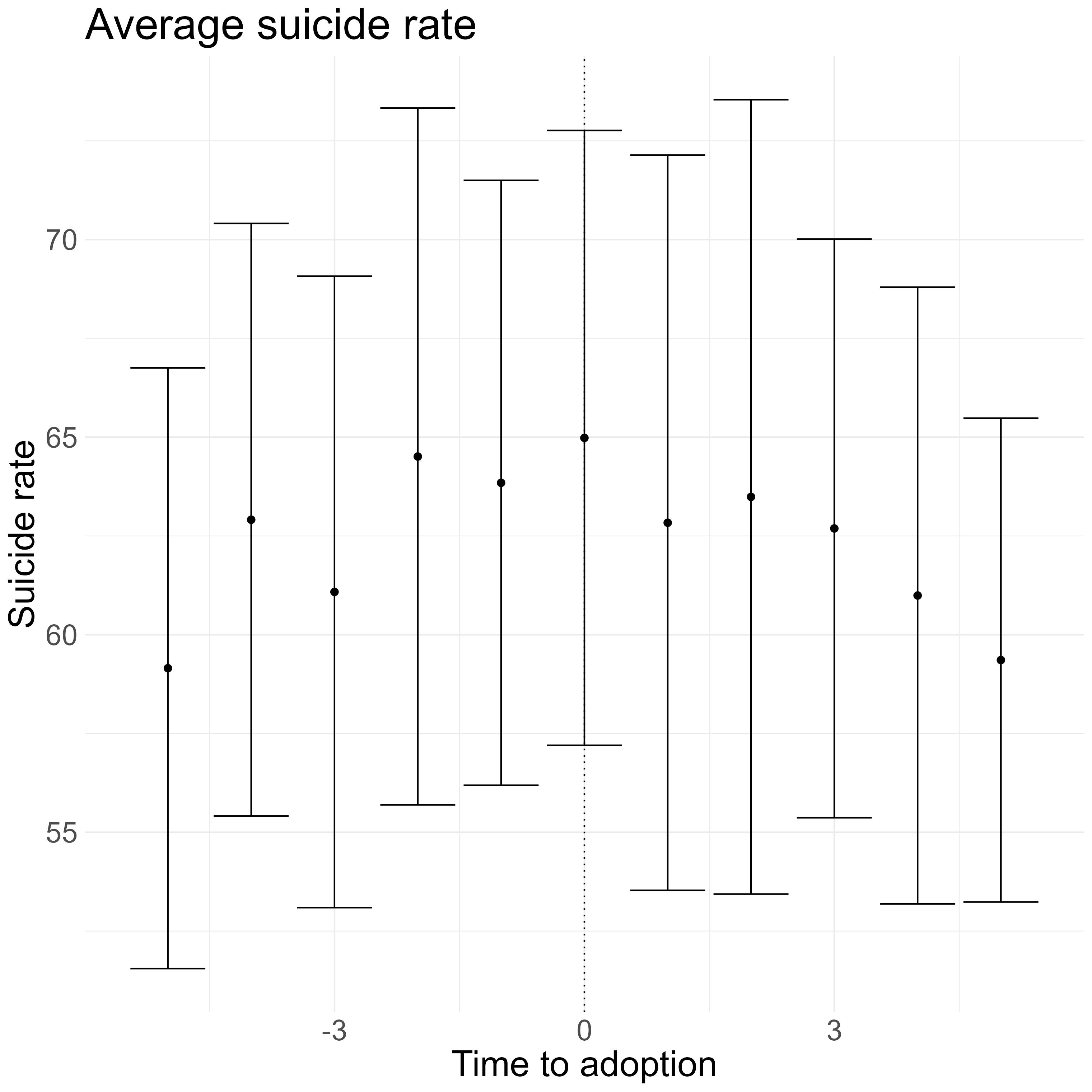
Figure 1: Average suicide rates across states as a function of time-to-adoption.

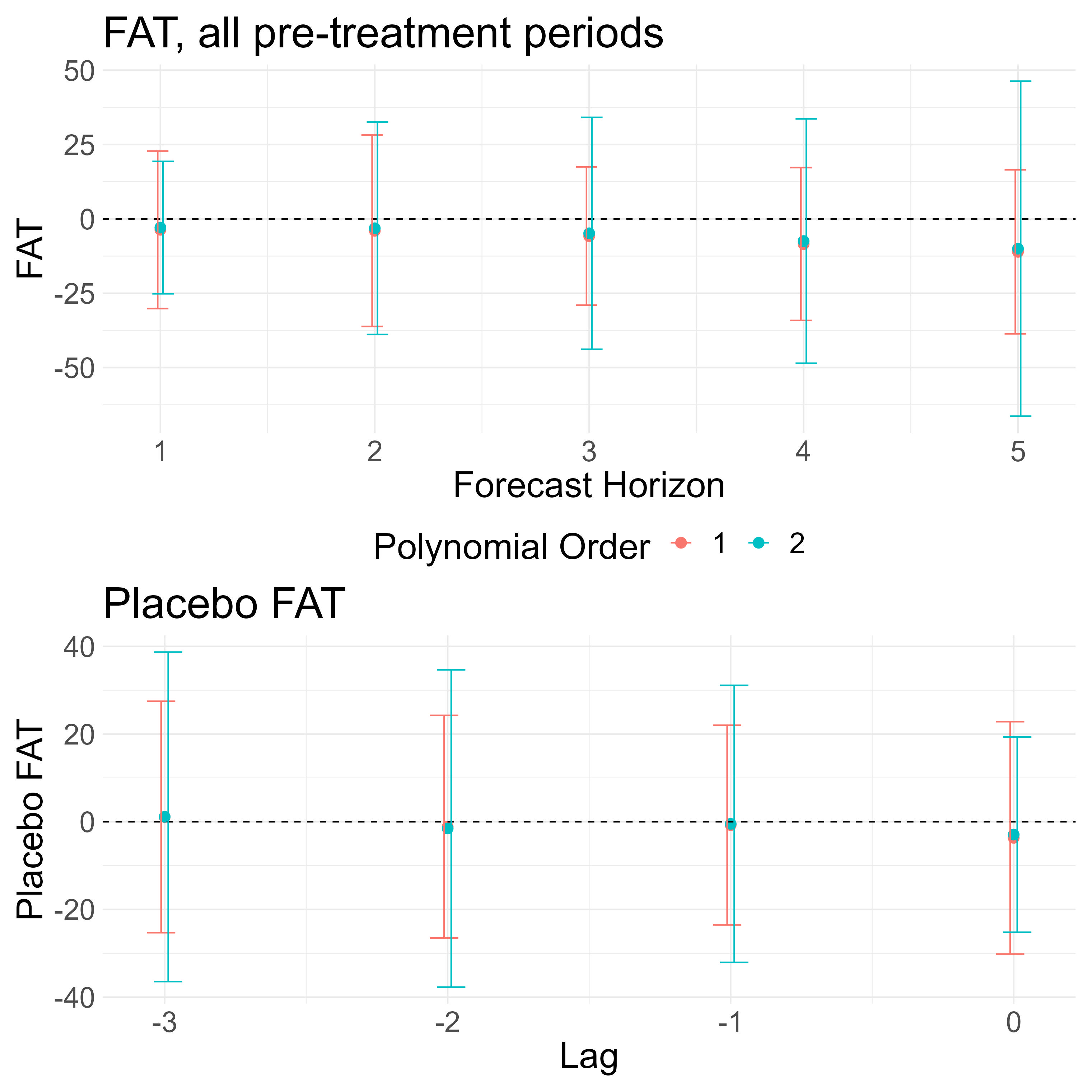
Figure 2: The top panel shows estimates of FAT for different forecast horizons (horizontal axis) and polynomial orders (different colors). The bottom panel shows estimates of placebo FAT (for $h=1$) as a function of the lag (horizontal axis) and polynomial order (different lines). Lag 0 is the actual adoption-year and placebo FAT at lag 0 is the FAT at forecast horizon 1 in the top panel. The error bars in both panels represent $95\%$ confidence intervals.

6 Conclusion

This paper proposed an estimator of the average treatment effects in the absence of a control group, based on forecasting individual counterfactuals using basis function regressions over a (short) time series of pre-treatment data. Forecast unbiasedness is a key requirement that is satisfied by our approach under a broad class of DGPs that express the individuals counterfactuals as the sum of up to three unobserved components: a stationary process, a stochastic trend, and a deterministic trend. The approach is robust, general and flexible, allowing for unbalanced panels, heterogeneous treatment effects, and staggered treatment timing. Forecasting counterfactuals using a model instead requires stronger assumptions and can perform poorly due to misspecification and estimation bias in small samples (e.g., incidental parameter problem).

Appendix A Proofs

Proof of Lemma 1.

We have

$$\widehat{{\rm FAT}}_{h}-{\rm ATT}_{h} =\frac{1}{n}\sum_{i=1}^{n}\left(y_{i\tau+h}-\widehat{y}_{i\tau+h}\left(0\right)-\mathbb{E}\left[y_{i\tau+h}-y_{i\tau+h}\left(0\right)\right]\right)$$

$$=\frac{1}{n}\sum_{i=1}^{n}\left(y_{i\tau+h}-\widehat{y}_{i\tau+h}\left(0\right)-\mathbb{E}\left[y_{i\tau+h}-\widehat{y}_{i\tau+h}\left(0\right)\right]\right)$$

$$=\frac{1}{n}\sum_{i=1}^{n}\left(u_{i\tau+h}-\mathbb{E}u_{i\tau+h}\right),$$

where we used Assumption 1 to obtain the second equality above. Since our assumptions guarantee that $\left(u_{i\tau+h}-\mathbb{E}u_{i\tau+h}\right)$ has zero mean and satisfies a CLT, we obtain the desired result. ∎

Proof of Theorem 1.

It is sufficient to show that for each component $y_{it}^{(r)}(0)$, $r\in\{1,2\}$,

$$\mathbb{E}\left[\sum_{t\in{\cal T}_{i}}\,w_{it}\,y_{it}^{(r)}-y_{i\tau+h}^{(r)}(0)\right] =0.$$ (30)

For both the mean stationary component ($r=1$) and the random walk component ($r=2$) we have $\mathbb{E}\left(y_{it}^{(r)}-y_{i\tau+h}^{(r)}(0)\right)=0$. Multiplying this equation by $w_{it}$, summing over $t\in{\cal T}_{i}$, and using the fact that the non-random weights $w_{it}$ sum to 1, we obtain (30) for $r=1$ and $r=2$. ∎

Proof of Lemma 2.

Let $R_{i}=q_{i}+1$ and $c_{s}\equiv\tau_{i}-R_{i}+s$, $s=1,2,\dots,R_{i}$. Define the $R_{i}\times\left(q_{i}+1\right)$ alternant matrix $X_{i}$ and the $1\times\left(q_{i}+1\right)$ vector $H_{i}$ as, respectively,

$$X_{i}\equiv\left[\begin{array}[]{cccc}1&b_{1}\left(c_{1}\right)&\dots&b_{q_{i}}\left(c_{1}\right)\\ 1&b_{1}\left(c_{2}\right)&\dots&b_{q_{i}}\left(c_{2}\right)\\ 1&b_{1}\left(c_{3}\right)&\dots&b_{q_{i}}\left(c_{3}\right)\\ \dots&\dots&\dots&\dots\\ 1&b_{1}\left(c_{\tau_{i}}\right)&\dots&b_{q_{i}}\left(c_{\tau_{i}}\right)\end{array}\right],\text{}H_{i}\equiv\left[\begin{array}[]{cccc}1&b_{1}\left(\tau+h\right)&\dots&b_{q_{i}+1}\left(\tau+h\right)\end{array}\right].$$ (31)

The OLS coefficients from regressing $y_{i}=\left(y_{i\tau_{i}-R_{i}+1},\dots,y_{i\tau_{i}}\right)$ on $b_{k}\left(t\right)$ are given by

$$\hat{\alpha}^{\left(q_{i},R_{i}\right)}=\left(X_{i}^{\prime}X_{i}\right)^{-1}X_{i}^{\prime}y_{i},$$

so that the $R_{i}$ forecast weights are

$$w_{i}=H_{i}\left(X_{i}^{\prime}X_{i}\right)^{-1}X_{i}^{\prime}.$$ (32)

Since $X_{i}$ is a Vandermonde matrix with the first column being a column of ones (by assumption), it follows that $X_{i}e_{1}=\iota.$ Then

$$\left(X_{i}^{\prime}X_{i}\right)^{-1}X_{i}^{\prime}\iota=e_{1}\equiv\left[\begin{array}[]{c}1\\ 0\\ \vdots\\ 0\end{array}\right],$$

so that $w_{i}\iota=1$, where $\iota$ is the $\left(q_{i}+1\right)\times 1$ vector of ones. This proves the statement. ∎

Proof of Theorem 2.

It is sufficient to show that for each component $y_{it}^{(r)}(0)$, $r\in\{1,2,3\}$,

$$\mathbb{E}\left[\sum_{t\in{\cal T}_{i}}\,w_{it}^{(q_{i},R_{i})}\,y_{it}^{(r)}-y_{i\tau+h}^{(r)}(0)\right] =0.$$ (33)

For the mean stationary component ($r=1$) and the random walk component ($r=2$) we have $\mathbb{E}\left(y_{it}^{(r)}-y_{i\tau+h}^{(r)}(0)\right)=0$. Multiplying this equation by $w_{it}^{(q_{i},R_{i})}$, summing over $t\in{\cal T}_{i}$, and using the fact that the non-random weights sum to 1 by Lemma 2, we obtain (33) for $r=1$ and $r=2$. To show (33) for the deterministic time trend component ($r=3$), note that by (10), $\sum_{t\in{\cal T}_{i}}w_{it}^{(q_{i},R_{i})}\,y_{it}^{(3)}=\sum_{k=0}^{q_{i}}\widetilde{c}_{ik}^{(q_{i},R_{i})}\,(\tau+h)^{k}$, where

$$\widetilde{c_{i}}^{(q_{i},R_{i})} :=\mathop{\mathrm{argmin}}_{c\in\mathbb{R}^{q_{i}+1}}\sum_{t\in{\cal T}_{i}}\left(y_{it}^{(3)}-\sum_{k=0}^{q_{i}}c_{k}\,b_{k}(t)\right)^{2}.$$

Since $q_{i}\geq q_{0i}$ for all $i$, the objective function in the last display is minimized (with value zero) at $\widetilde{c}_{ik}^{(q_{i},R_{i})}=c_{ik}^{(3)}$, which implies $y_{i\tau+h}^{(3)}(0)=\sum_{t\in{\cal T}_{i}}\,w_{it}^{(q_{i},R_{i})}\,y_{it}^{(3)}$, that is, (33) holds for $r=3$ even without taking the expectation. ∎

Proof of Theorem 3.

We have

$$\widehat{{\rm FAT}}_{h}^{\rm MB}-{\rm ATT}_{h}$$

$$=\frac{1}{n}\sum_{i=1}^{n}\left(y_{i\tau+h}-\widehat{y}_{h}(\widehat{\beta},y_{i},x_{i})-\mathbb{E}\left[y_{i\tau+h}-y_{i\tau+h}\left(0\right)\right]\right)$$

$$=\frac{1}{n}\sum_{i=1}^{n}\left(y_{i\tau+h}-\widehat{y}_{h}(\widehat{\beta},y_{i},x_{i})-\underbrace{\mathbb{E}\left[y_{i\tau+h}-\widehat{y}_{h}(\beta_{0},y_{i},x_{i})\right]}_{=\mathbb{E}\left[u_{i\tau+h}^{*}\right]}\right)$$

$$=\frac{1}{n}\sum_{i=1}^{n}\left[y_{i\tau+h}-\widehat{y}_{h}(\beta_{0},y_{i},x_{i})-\frac{\partial\widehat{y}_{h}(\beta_{0},y_{i},x_{i})}{\partial\beta^{\prime}}\left(\widehat{\beta}-\beta_{0}\right)\right]-\mathbb{E}\left[u_{i\tau+h}^{*}\right]$$

$$\qquad+O\left(R_{n}\left\|\widehat{\beta}-\beta_{0}\right\|^{2}\right)$$

$$=\frac{1}{n}\sum_{i=1}^{n}u_{i\tau+h}^{*}-\mathbb{E}\left[u_{i\tau+h}^{*}\right]+O\left(R_{n}\left\|\widehat{\beta}-\beta_{0}\right\|^{2}\right)$$

$$\qquad-\left\{\frac{1}{n}\sum_{i=1}^{n}\frac{\partial\widehat{y}_{h}(\beta_{0},y_{i},x_{i})}{\partial\beta^{\prime}}-\frac{1}{n}\sum_{j}\mathbb{E}\left[\frac{\partial\widehat{y}_{h}(\beta_{0},y_{j},x_{j})}{\partial\beta^{\prime}}\right]\right\}\left(\widehat{\beta}-\beta_{0}\right)$$

$$\qquad-\frac{1}{n}\sum_{j}\mathbb{E}\left[\frac{\partial\widehat{y}_{h}(\beta_{0},y_{j},x_{j})}{\partial\beta^{\prime}}\right]r_{n}$$

$$=\frac{1}{n}\sum_{i=1}^{n}u_{i\tau+h}^{*}-\mathbb{E}\left[u_{i\tau+h}^{*}\right]+o_{P}(n^{-1/2})$$

Here, in the first step, we plugged in the definitions of $\widehat{{\rm FAT}}_{h}^{\rm MB}$ and ${\rm ATT}_{h}$. In the second step, we used the unbiasedness of the forecast, definition (26), and assumption (iii) that $\mathbb{E}\left(\psi(y_{i},x_{i})\right)=0$. In the third step, given assumption (ii), we employed a Taylor expansion of $\widehat{y}_{h}(\beta,y_{i},x_{i})$ in $\beta$ around $\beta_{0}$. In the fourth step we decomposed $\frac{\partial\widehat{y}_{h}(\beta_{0},y_{i},x_{i})}{\partial\beta^{\prime}}$ into its expectation and its deviation from the expectation, and used $\widehat{\beta}-\beta_{0}=\frac{1}{n}\sum_{i=1}^{n}\psi(y_{i},x_{i})+r_{n}$ and the definition of $u_{i\tau+h}^{*}$ in (26). In the final step, we used our assumptions to conclude that the various remainder terms are all of order $o_{P}(n^{-1/2})$. By an application of a standard cross-sectional CLT we then obtain the conclusion of the theorem. ∎

Appendix B Estimating the variance of $\widehat{{\rm FAT}}_{h}$

According to Lemma 1 the asymptotic variance of $\sqrt{n}\widehat{{\rm FAT}}_{h}$ is given by $\bar{\sigma}^{2}_{n}:={\rm Var}(\frac{1}{\sqrt{n}}\sum_{i}u_{i\tau+h})$, which under cross-sectional independence can be consistently estimated by

$$\frac{1}{n}\sum_{i=1}^{n}\left(u_{i\tau+h}-\overline{u}_{\tau+h}\right)^{2},$$

where $\overline{u}_{\tau+h}=\frac{1}{n}\sum_{i=1}^{n}u_{i\tau+h}$, with $u_{i\tau+h}:=y_{i\tau+h}-\widehat{y}_{i\tau+h}(0)$.

If an additional unknown common parameter $\beta_{0}$ needs to be estimated, then the uncertainty of the estimator $\widehat{\beta}$ also becomes relevant. In that case, according to Theorem 3, the asymptotic variance of $\sqrt{n}\widehat{{\rm FAT}}_{h}$ is $\bar{\sigma}^{*2}_{n}:={\rm Var}\left(\frac{1}{\sqrt{n}}\sum_{i}u^{*}_{i\tau+h}\right)$, where $u^{*}_{i\tau+h}:=y_{i\tau+h}-\widehat{y}_{h}(\beta_{0},y_{i},x_{i})-\frac{1}{n}\sum_{j=1}^{n}\mathbb{E}\left[\frac{\partial\widehat{y}_{h}(\beta_{0},y_{j},x_{j})}{\partial\beta^{\prime}}\right]\psi(y_{i},x_{i})$. Here, both $\beta_{0}$ and the influence function $\psi(y_{i},x_{i})$ of $\widehat{\beta}$ are unknown. For example, if $\widehat{\beta}$ is a method of moment estimator (which includes OLS, MLE, and exactly identified IV) that solves the sample moment condition

$$\sum_{i=1}^{n}g(y_{i},x_{i},\widehat{\beta})=0,$$

then, assuming that $g(y_{i},x_{i},\beta)$ is sufficiently often differentiable in $\beta$, we have

$$\psi(y_{i},x_{i})=\left(\frac{1}{n}\sum_{j=1}^{n}\frac{\partial^{2}g(y_{j},x_{j},\beta_{0})}{\partial\beta\partial\beta^{\prime}}\right)^{-1}\frac{\partial g(y_{i},x_{i},\beta_{0})}{\partial\beta},$$

which can be estimated by

$$\widehat{\psi}(\widehat{\beta},y_{i},x_{i})=\left(\frac{1}{n}\sum_{j=1}^{n}\frac{\partial^{2}g(y_{j},x_{j},\widehat{\beta})}{\partial\beta\partial\beta^{\prime}}\right)^{-1}\frac{\partial g(y_{i},x_{i},\widehat{\beta})}{\partial\beta}.$$

In that case, we can estimate $u^{*}_{i\tau+h}$ by

$$\widehat{u}^{*}_{i\tau+h}=y_{i\tau+h}-\widehat{y}_{h}(\widehat{\beta},y_{i},x_{i})-\left(\frac{1}{n}\sum_{j=1}^{n}\ \frac{\partial\widehat{y}_{h}(\beta_{0},y_{j},x_{j})}{\partial\beta^{\prime}}\right)\widehat{\psi}(\widehat{\beta},y_{i},x_{i}),$$

and a consistent estimator for $\bar{\sigma}^{*2}_{n}$ is given by

$$\frac{1}{n}\sum_{i=1}^{n}\left(\widehat{u}^{*}_{i\tau+h}-\overline{\widehat{u}}^{*}_{\tau+h}\right)^{2},$$

where $\overline{\widehat{u}}^{*}_{\tau+h}=\frac{1}{n}\sum_{i=1}^{n}\widehat{u}^{*}_{i\tau+h}$. If $\widehat{\beta}$ is not a method of moment estimator (e.g., it is a more general GMM estimator), then the formula for $\widehat{\psi}(\widehat{\beta},y_{i},x_{i})$ needs to be generalized accordingly, but the final estimation of $\bar{\sigma}^{*2}_{n}$ by the sample variance of $\widehat{u}^{*}_{i\tau+h}$ remains unchanged.

Appendix C Online Appendix

The Online Appendix contains extensions, additional simulations and empirical replications. In the main text, we consider FAT under the assumption that the class of DGPs for the counterfactuals does not include common unforecastable shocks. We show how this assumption can be relaxed when there exists another variable that is subject to the same common shock but not to the treatment (in Online Appendix C.1) or when there exists a control group that is subject to the common shock (in Online Appendix C.2). The simulations in the main text consider the case of homogeneous time trends and autoregressive parameters. We relax this in Online Appendix C.3. Finally, we present two additional empirical applications in Online Appendix C.4 and C.5.

C.1 Extension: no control group, common shock

We sketch here a possible way to weaken the assumption of no forecastable shock between treatment time $\tau$ and forecast time $\tau+h,h\geq 1$.

Let $\widetilde{y}_{it}\left(0\right)$ follow either Assumption 3 or 4 and let $W_{it}$ be another observed variable that is affected by a shock $\gamma_{t}$ but not by the treatment. Suppose that

$$y_{it}\left(0\right) =\gamma_{t}1\left(t>\tau\right)+\widetilde{{y}}_{it}\left(0\right),$$ (34)

$$W_{it} =\theta_{i}^{W}\gamma_{t}1\left(t>\tau\right)+\epsilon_{it}.$$ (35)

Denote by $\widehat{\gamma}_{t}$ the estimator of $\gamma_{t}$ obtained from post-treatment data on $W_{it},$ $t>\tau$ via, e.g., PCA. Then

$$\widehat{{\rm FAT}}_{h} =\frac{1}{n}\sum_{i}\left(y_{i\tau+h}-\widehat{\widetilde{y}}_{i\tau+h}\left(0\right)\right)-\widehat{\gamma}_{\tau+h},$$ (36)

where $\widehat{\widetilde{y}}_{i\tau+h}(0)$ is the couterfactual forecast obtained as before via basis function regression.

C.2 Extension: control group

In this section, we discuss how to modify our baseline procedure when a group of individuals not exposed to the treatment is available.

Without a control group, Section 2 derived sufficient conditions ensuring that ${\rm FAT}_{h}$ defined in (6) is a consistent and asymptotically normal estimator of ${\rm ATT}_{h}$ defined in (4). These conditions are the ability to obtain forecasts of the counterfactuals using pre-treatment data that are on average unbiased (Assumption 1) and the validity of a central limit theorem (Assumption 2). As discussed in the main text, these conditions exclude the presence of time effects such as macro shocks that affect all individuals between times $\tau$ and $\tau+h$, $h\geq 1$, and that are unforecastable using pre-treatment data. The presence of a control group allows us to weaken this assumption.

C.2.1 DFAT: FAT with a control group

Suppose that all individuals are untreated before the implementation of the treatment at time $\tau$ and that some individuals remain untreated after $\tau$. Let $D_{i}=1$ if individual $i$ is untreated before and after $\tau$. The observed outcome of individual $i$ at time $t$ is then

$$y_{it}=D_{i}\left[1\left(t\leq\tau\right)y_{it}\left(0\right)+1\left(t>\tau\right)y_{it}\left(1\right)\right]+\left(1-D_{i}\right)y_{it}\left(0\right).$$ (37)

As before, the parameter of interest is the average treatment effect on the treated $h$ periods after the implementation of the treatment:

$${\rm ATT}_{h}=\frac{1}{n}\sum^{n}_{i=1}\mathbb{E}\left(\left.y_{i\tau+h}\left(1\right)-y_{i\tau+h}\left(0\right)\right|D_{i}=1\right).$$ (38)

Our proposed estimator is defined as:

$$\widehat{\rm DFAT}_{h}=\frac{1}{n_{1}}\sum_{i:D_{i}=1}(\left.y_{i\tau+h}-\widehat{y}_{i\tau+h}(0)\right)-\frac{1}{n_{0}}\sum_{i:D_{i}=0}(\left.y_{i\tau+h}-\widehat{y}_{i\tau+h}(0)\right),$$ (39)

where $n_{1}$ is the number of treated individuals at time $\tau+h$, $n_{0}$ is the number of control individuals at time $\tau+h$, and $y_{i\tau+h}$ is the observed outcome at $\tau+h$ given by (37).

Note that under (40) below, $\mathbb{E}(\widehat{\rm DFAT}_{h})={\rm ATT}_{h}$ in (38):

$$\frac{1}{n}\sum^{n}_{i=1}\mathbb{E}\left(\left.y_{i\tau+h}\left(0\right)-\widehat{y}_{i\tau+h}(0)\right|D_{i}=1\right)=\frac{1}{n}\sum^{n}_{i=1}\mathbb{E}\left(\left.y_{i\tau+h}\left(0\right)-\widehat{y}_{i\tau+h}(0)\right|D_{i}=0\right).$$ (40)

Unlike in the baseline case, the forecast $\widehat{y}_{i\tau+h}(0)$ can be biased, as long as the average bias for the treated group equals the average bias for the control group. As a consequence, the DGP for $y_{it}(0)$ can contain additive time effects that are common across individuals such as additive macro shocks that affect both treated and control groups in the same way.

The presence of a control group allows us to substitute Assumption 4 to allow for a common shock that is not necessarily polynomial, e.g., $y_{it}\left(0\right)=\tilde{y}_{it}(0)+\gamma_{t}$, where $\tilde{y}_{it}(0)$ satisfies Assumption 4. Then, under assumptions similar to Assumptions 1 and 2, it is possible to show consistency and asymptotic normality of (39).

As in Section 2 in the main text, we suggest using $\widehat{y}_{i\tau+h}^{(q_{i},R_{i})}(0)$ as an estimator for $\widehat{y}_{i\tau+h}(0)$ in (39). Here, the parameters $q_{i},R_{i}$ do not necessarily have to be the same for the treated and control units.

C.2.2 Comparison with Difference-in-Differences

Despite the apparent similarity with the difference-in-differences (DiD) framework, our method in the presence of a control group allows for DGPs for counterfactuals with more general forms of latent heterogeneity. For example, our approach allows for counterfactuals that follow fully heterogeneous autoregressive processes and/or unit root processes. In addition, it allows for the DGPs to have additive individual-specific time trends, as long as the deterministic time trend is either known or can be approximated by, e.g., a polynomial.

To see this, consider for example the following DGP for the counterfactuals:

$$y_{it}\left(0\right)=\rho y_{it-1}\left(0\right)+\gamma_{t}+k_{i}t+\epsilon_{it},\mathbb{E}\left(\epsilon_{it}\right)=0,$$

where $\rho\in[0,1]$, $\gamma_{t}$ is a common shock and $k_{i}$ is an individual-specific time trend coefficient.

DiD can accommodate such specifications as long as the assumption of parallel-paths holds, which requires restricting the heterogeneity of both the initial condition, i.e.,

$$\frac{1}{n}\sum^{n}_{i=1}\mathbb{E}(\left.y_{i0}(0)\right|D_{i}=1)=\frac{1}{n}\sum^{n}_{i=1}E(\left.y_{i0}(0)\right|D_{i}=0)$$

and the time trend coefficients, i.e.,

$$\frac{1}{n}\sum^{n}_{i=1}k_{i}I\left(D_{i}=1\right)=\frac{1}{n}\sum^{n}_{i=1}k_{i}I\left(D_{i}=0\right),$$

where $I(\cdot)$ is the indicator function.

In contrast, ${\rm DFAT}_{h}$ does not require restricting the unobserved individual heterogeneity, and allows for heterogeneous $k_{i}$. In addition, it is straightforward to include lagged pre-treatment covariates with a homogeneous autoregressive parameter or a heterogeneous one, which is generally considered problematic in DiD methods.

In addition, our paradigm of first obtaining individual-specific forecasts and only afterwards averaging across individuals avoids any concern about estimating weighted as opposed to unweighted treatment effects. It is well known that for unbalanced panels and for staggered adoption designs the DiD method will estimate a weighted average of the individual specific treatment effects with weights that are determined implicitly by the regression design, and that may even be negative in some cases (see e.g. deChaisemartinX2020,GoodmanBacon). By contrast, FAT (or DFAT) explicitly gives a weight of $1/n$ (or $1/n_{d}$) to each individual by construction, in accordance with the unweighted treatment effect that is specified as estimand.

C.2.3 Related literature

Conceptually, when there exists a control group, our solution resembles difference-in-differences or, more generally, an “event-study design analysis”, e.g., Borusyaketal2021. Although the estimated outcome equations may look similar, there is an important distinction between these methods and ours. For example, the extension of FAT to the case of a control group (which we call DFAT) uses control groups to correct for the effect of a common shock, whereas the other methods use control groups to correct for selection into treatment (under different assumptions). Additionally, FAT allows for heterogeneous time trends as well as for heterogeneous effects of lagged pre-treatment outcomes. In contrast, there is no straightforward way to control for pre-treatment lagged outcomes in the specifications of, e.g., SunAbraham, CallawaySantAnna, Borusyaketal2021.

The synthetic control method has been increasingly used to evaluate the effect of interventions implemented at an aggregate level, see Abadie2021 for a recent review. In the conventional setting for synthetic controls, there is only one unit that is treated and there are many untreated units that could be used as pseudo-controls, i.e. these are untreated units selected such that the weighted average of their past outcomes “resembles” the trajectory of past outcomes of the treated unit. The counterfactual outcome for the treated unit is then constructed as a weighted average of the post-treatment outcomes of the selected pseudo-control units. In comparison, in our baseline setting, all individuals in the population are treated and there are no control units. The counterfactual outcome for each treated unit is a weighted average of the unit’s own past outcomes. The properties of our estimator rest on averaging across many treated units, an advantage of which is standard inference. Our results apply even when the number of pre-treatment time periods is small, and we fully characterize the class of DGPs that obtains a consistent estimator of the ATT.

Imputing counterfactual outcomes for the treated from data on the control is used in the literature on matrix completion, e.g., athey2021matrix, bai2019matrix, fernandez2020low. Our framework has a thin matrix of outcomes. However since we do not observe cross-sectional control units, we cannot appeal to these methods to impute the counterfactuals.

C.3 Simulation: Heterogeneous coefficients

We compare the finite-sample behavior of the polynomial-regression FAT when the counterfactual process satisfies Assumption 4 with heterogeneous coefficients $\rho_{i}$ and $\delta_{i}$. That is, we consider the same specification of $y_{it}(0)$ as in Section 4.2 with $I_{1}=I_{2}=I_{3}=1$, with the only changes being that $\rho_{i}$ and $\delta_{i}$ vary across individuals.

Table 3 presents the results for $\delta_{i}\sim\mathcal{U}\left[0,2\right]$ with a homogeneous autoregressive parameter $\rho=0.2$ (top panel) and with a heterogeneous autoregressive parameter $\rho_{i}\sim\mathcal{U}\left[0,0.99\right]$ (bottom panel). We can see that the presence of heterogeneous parameters does not change the conclusions that we derived from Table 2.

		$R_{i}$
		$q+1$	$q+2$	$q+3$	$q+4$	$q+5$
Stationary AR(1) $I_{1}=I_{2}=I_{3}=1$ with $\delta_{i}\sim\mathcal{U}[0,2]$	$q=0$
	bias	0.999	1.4987	2.0003	2.5012	3.0015
	s.e.	0.0544	0.0585	0.0655	0.0739	0.0826
	$q=1$
	bias	0.0013	0.0038	0.0009	0
	s.e.	0.0793	0.0666	0.0646	0.0635
	$q=2$
	bias	-0.0024	0.0065	0.0045
	s.e.	0.1437	0.0971	0.0846
Stationary AR(1) $I_{1}=I_{2}=I_{3}=1$ with $\delta_{i}\sim\mathcal{U}[0,2]$ and $\rho_{i}\sim\mathcal{U}[0,0.99]$	$q=0$
	bias	0.9967	1.4961	1.9963	2.4958	2.9947
	s.e.	0.0554	0.0613	0.0693	0.078	0.0861
	$q=1$
	bias	-0.0002	0.001	0.0027	0.0035
	s.e.	0.0717	0.0629	0.0643	0.0672
	$q=2$
	bias	0.0019	-0.0023	-0.0005
	s.e.	0.1264	0.0929	0.0801

Table 3: Bias and standard error (s.e.) for the polynomial-regression FAT when the counterfactual is specified as in the left-most column. The time trend component is heterogeneous across individuals (top panel), with the addition of a cross-sectionally heterogeneous autoregressive component (bottom panel). Stationary initial condition for the AR($1$) component for each $i$.

C.4 Empirical replication: Overdose mortality and medical cannabis laws

We use data from Shover to analyze the effect of adopting legalized medical cannabis laws on opioid overdose mortality in the US. Shover contributes to the debate about whether the adoption of such laws has decreased overdose mortality, see, e.g., Bachuber.

The unit of observation is at the level of state-year, with states adopting legalized medical cannabis laws from 1999 to 2017. Our analysis includes $n=$34 states that legalized medical cannabis during that period. The outcome of interest is the log mortality rate.

Both Bachuber and Shover use two-way fixed-effects estimators to analyze the effects of adopting legalized medical cannabis laws. In a staggered adoption setting, this estimation method produces biased results, e.g. Goodman-Bacon (2021). Therefore, we first redo the analysis to remove the bias of the original studies by using various methods, such as the staggered DiD approach of CallawaySantAnna and the generalized synthetic control method of Xu. Figure 3 uses the method of Callaway and Sant’Anna (2021) with not-yet-treated-states as control units, while Figure 4 uses the method of Xu to impute counterfactuals for each treated unit using a linear two-way fixed effects regression. This analysis finds an initial increase in overdose mortality and then a reversal, but neither is statistically significant.

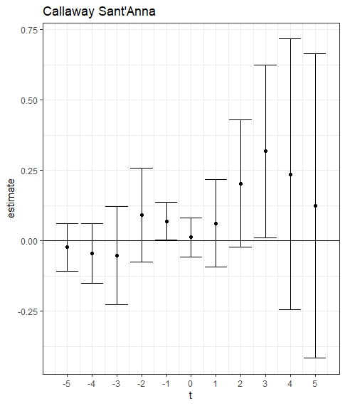
Figure 3: Overdose mortality rate as a function of time to adoption using not-yet-treated-states as control units.

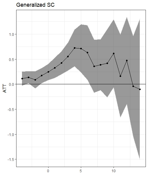
Figure 4: Overdose mortality rate as a function of time to adoption via generalized SC.

We then implement FAT. We start with a plot of the log mortality rate averaged across states as a function of time to adoption; see Figure 5, in order to get a sense for the time series properties of the outcome of interest. The outcome appears to be non-stationary over the pre-treatment period, so we choose the smallest possible estimation window $R=q+1$ to calculate FAT (as in (29)) and let the order of the polynomial be $q=1,2$. The top panel of Figure 6 shows our FAT estimates for the ATT as a function of the forecast horizon. Our estimates are stable across the polynomial orders, and our results show a slight increase in the overdose mortality rate. However, the increase does not appear to be statistically significant across the forecast horizon. Our results thus corroborate those of the approaches of CallawaySantAnna and Xu, but without using a control group.

We also compute placebo FAT by assuming that the law was adopted by each state either one year earlier or two years earlier, respectively, in the bottom panel of Figure 6. We consider these values because FAT in the top panel is computed using the outcome either one period before adoption (when $q=1$) or two periods before adoption (when $q=2$). Figure 6 shows the placebo FAT estimates computed with $R=q+1$, $q=1,2$. The forecast horizon is $h=1$, so the placebo FAT at lag 0 corresponds to FAT at forecast horizon 1 in the top panel. The figure shows that the estimated placebo FATs are statistically insignificant. Although this is not a test of our assumptions, these placebo estimates offer suggestive evidence that FAT estimates may be interpreted as the ATT across different forecast horizons.

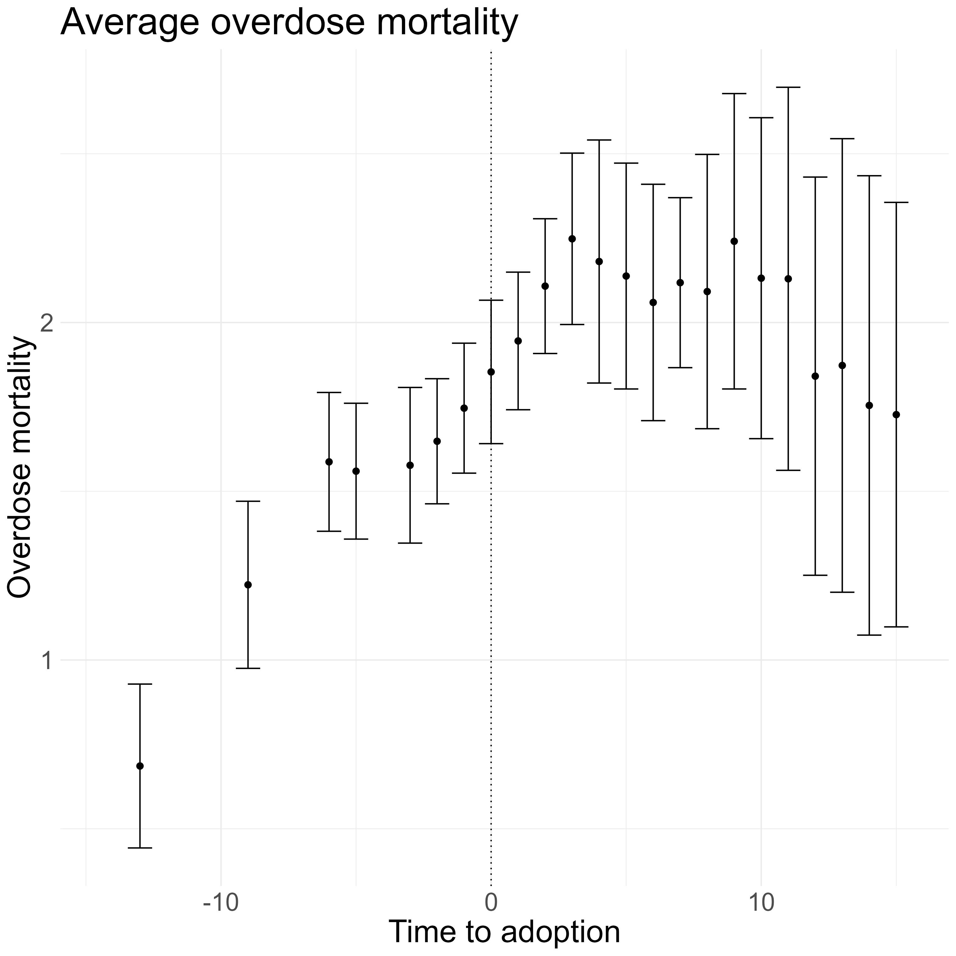
Figure 5: Log mortality rate averaged across states as a function of time-to-adoption.

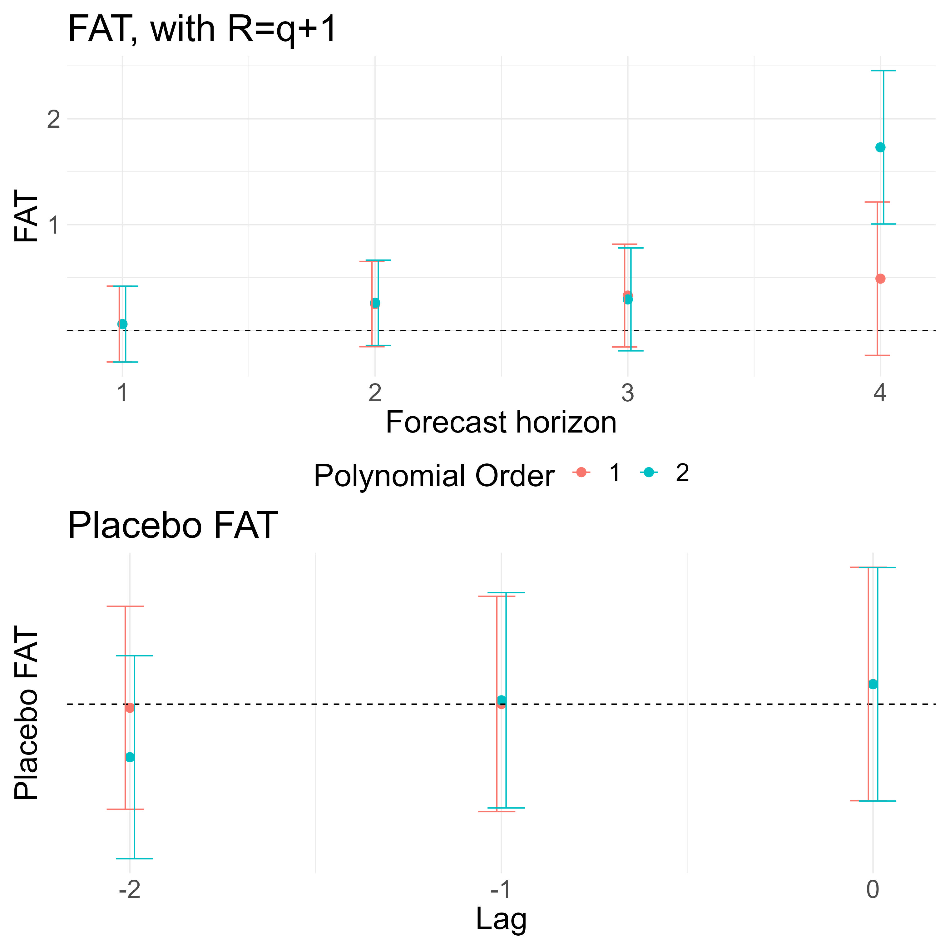
Figure 6: The effect of adopting legalized marijuana laws on overdose mortality rate. The top panel shows estimates of FAT as a function of forecast horizon (horizontal axis) and polynomial order (colored lines). FAT is computed with a variable number of pre-treatment time periods, $R=q+1,q=1,2$. The bottom panel shows estimates of placebo FAT as a function of lag (horizontal axis) and polynomial order (colored lines). Lag 0 is the actual adoption year. Placebo FAT is computed with a variable number of pre-treatment time periods, $R=q+1,q=1,2$.

C.5 Empirical replication: Refugees and far-right support

In this replication exercise, we use data from Dinas which examines the relationship between refugee arrivals and support for the far right. Dinas consider the case of Greece, and make use of the fact that some Greek islands (those close to the Turkish border) witnessed sudden and unexpected increases in the number of refugees during the summer of 2015, while other nearby Greek islands saw much more moderate inflows of refugees. The municipalities in the former Greek islands are considered treated, while the municipalities in the latter are considered controls. The authors use a standard DiD analysis to assess whether the treated municipalities were more supportive of the far-right Golden Dawn party in the September 2015 general election. The original data set contains a total of 96 municipalities, $48$ of which were treated, and data on four elections: three elections pre-treatment in 2012, 2013, 2015, and one post-treatment in 2016. The outcome of interest is the vote share for Golden Dawn (GD). Figure 7 shows the vote share for GD averaged across municipalities, treated and control, before and after the treatment time.

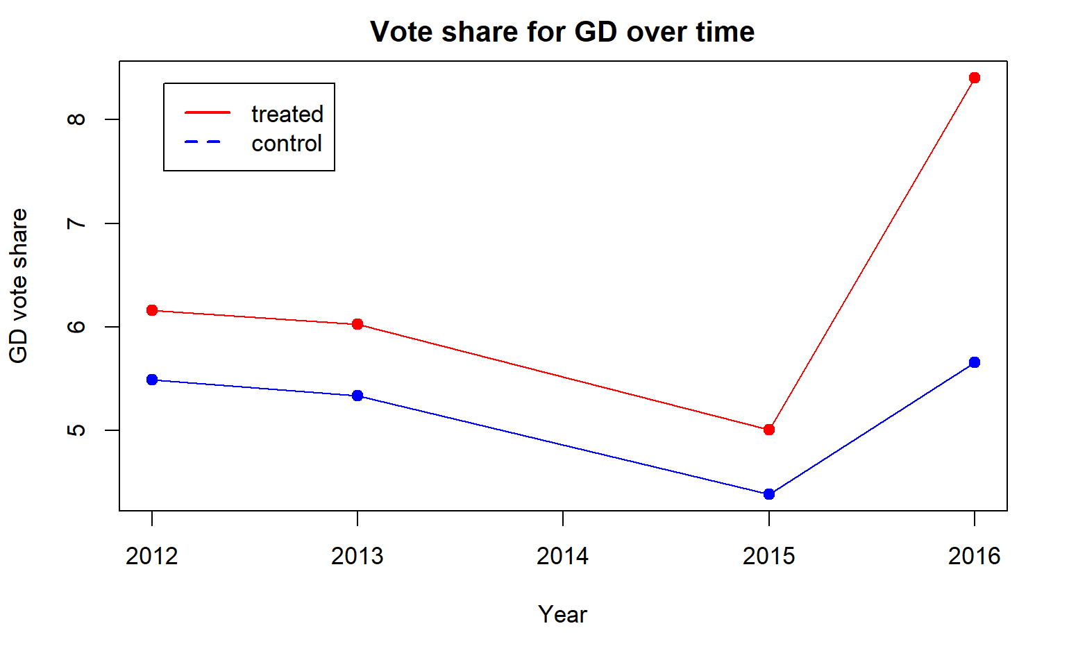
Figure 7: Vote share for Golden Dawn averaged across municipalities before and after $2015$ for municipalities that were treated (red) and control (blue).

We use data on both the treated and the control municipalities to compute $\widehat{\rm{DFAT}}_{h}$ in equation (39) with $h=1$ and show that our estimate replicates the original DiD estimates. This application can be viewed as a “worst-case” scenario for our proposed estimator since the number of treated units is very small. We show results that use all three pre-treatment elections, in which case the order of the polynomial is $q_{i}=q\in\left\{0,1,2\right\}$, and results that use only the $2013$ and $2015$ pre-treatment elections, in which case the order of the polynomial is $q_{i}=q\in\left\{0,1\right\}$. Note that we perform municipality-specific polynomial regressions to compute the forecasted vote share – the counterfactual outcome of interest, using the same polynomial order across all municipalities.

As Table 4 shows, our DFAT results are comparable with those in the original paper. The DiD estimates in the original paper are $0.0206$ and $0.0208$ when using $2013$ and $2015$ as pre-treatment periods and all pre-treatment periods, respectively. The two-way fixed-effects estimate is $0.021$ with a standard error of $0.0393$.

We include here placebo FAT estimates which we compute by assuming that the treatment took place in $2015$. The point here is to assess if the estimated placebo FAT is statistically not different from zero. We use a polynomial of degree $q=0$ when the pre-treatment year is $2013$ and a polynomial of degree $q=1$ when the pre-treatment years are $2012$ and $2013$. The placebo FATs are all statistically insignificant: the placebo FAT for the treated when $q=0$ is $-0.010$ with a standard error of $0.013$, while when $q=1$ it is $-0.009$ with a standard error of $0.029$. The placebo FAT for the control when $q=0$ is $-0.010$ with a standard error of $0.012$, while when $q=1$ it is $-0.008$ with a standard error of $0.017$. The corresponding placebo DFAT’s are then: $0$ for $q=1$ with a standard error of $-0.001$ and $0.016$ for $q=1$ with a standard error of $0.034$.

	FAT Treated	FAT Control	DFAT
Polynomial order	2013-2015
$q=0$	0.029 (0.016)	0.008 (0.009)	0.021
$q=1$	0.054 (0.028)	0.032 (0.026)	0.022
	2012-2015
$q=0$	0.027 (0.012)	0.006 (0.011)	0.021
$q=1$	0.038 (0.025)	0.017 (0.016)	0.019
$q=2$	0.053 (0.036)	0.030 (0.027)	0.023

Table 4: DFAT under different polynomial orders and pre-treatment periods.

References

- Abouk and Adams (2013) Abouk, R. and S. Adams (2013). Texting bans and fatal accidents on roadways: Do they work? or do drivers just react to announcements of bans? American Economic Journal: Applied Economics 5(2), 179–199.
- Angrist and Pischke (2009) Angrist, J. and J. Pischke (2009). Mostly harmless econometrics. Princeton University Press.
- Arkhangelsky and Imbens (2023) Arkhangelsky, D. and G. Imbens (2023). Causal models for longitudinal and panel data: A survey. NBER Working Paper No. 31942.
- Baker et al. (2008) Baker, M., J. Gruber, and K. Milligan (2008). Universal child care, maternal labor supply, and family well-being. Journal of Political Economy 116, 709–745.
- Baltagi (2013) Baltagi, B. H. (2013). Chapter 18 - panel data forecasting. In G. Elliott and A. Timmermann (Eds.), Handbook of Economic Forecasting, Volume 2 of Handbook of Economic Forecasting, pp. 995–1024. Elsevier.
- Bernal et al. (2017) Bernal, J. L., S. Cummins, and A. Gasparrini (2017). Interrupted time series regression for the evaluation of public health interventions: a tutorial. International Journal of Epidemiology 46(1), 348–355.
- Blundell et al. (2004) Blundell, R., C. Meghir, M. Costa Dias, and J. Van Reenen (2004). Evaluating the employment impact of a mandatory job search program. Journal of the European Economic Association 2(4), 569–606.
- Brodersen et al. (2015) Brodersen, K., F. Gallusser, J. Koehler, N. Remy, and S. L. Scott (2015). Inferring causal impact using bayesian structural time-series models. Annals of Applied Statistics 1(9), 247–274.
- Brown and Warner (1985) Brown, S. and J. Warner (1985). Using daily stock returns: The case of event studies. Journal of Financial Economics 14(1), 3–31.
- Cerqua et al. (2023) Cerqua, A., M. Letta, and F. Menchetti (2023). The machine learning control method for counterfactual forecasting. https://ssrn.com/abstract=4315389.
- Chernozhukov et al. (2013) Chernozhukov, V., I. Fernández-Val, J. Hahn, and W. Newey (2013). Average and quantile effects in nonseparable panel models. Econometrica 81(2), 535–580.
- Chernozhukov et al. (2021) Chernozhukov, V., K. Wuethrich, and Y. Zhu (2021). An exact and robust conformal inference method for counterfactual and synthetic controls. Journal of the American Statistical Association 116(536), 1849–1864.
- Clarke and Tapia-Schythe (2021) Clarke, D. and K. Tapia-Schythe (2021). Implementing the panel event study. The Stata Journal 21(4), 853–884.
- de Chaisemartin and D’Haultfoeuille (2020) de Chaisemartin, C. and X. D’Haultfoeuille (2020). Two-way fixed effects estimators with heterogeneous treatment effects. American Economic Review 110(9), 2964–2996.
- Dufour (1984) Dufour, J.-M. (1984). Unbiasedness of predictions from estimated autoregressions when the true order is unknown. Econometrica 52(1), 209–216.
- Fuller and Hasza (1980) Fuller, W. and D. Hasza (1980). Predictors for the first-order autoregressive process. Journal of Econometrics 13(2), 139–157.
- Gallego et al. (2013) Gallego, F., J.-P. Montero, and C. Salas (2013). The effect of transport policies on car use: Evidence from latin american cities. Journal of Public Economics 107, 47–62.
- Ghanem et al. (2022) Ghanem, D., P. Sant’Anna, and K. Wuthrich (2022). Selection and parallel trends. CESifo Working Paper No. 9910.
- Goodman-Bacon (2021) Goodman-Bacon, A. (2021). Difference-in-differences with variation in treatment timing. Journal of Econometrics 225(2), 254–277.
- Heckman and Vytlacil (2005) Heckman, J. and E. Vytlacil (2005). Econometric evaluation of social programs. In J. Heckman and E. Leamer (Eds.), Handbook of Econometrics, Volume 6. Amsterdam: Elsevier Science.
- Hirano and Imbens (2001) Hirano, K. and G. Imbens (2001). Estimation of causal effects using propensity score weighting: An application to data on right heart catheterization. Health Services & Outcomes Research Methodology 2, 259–278.
- Jorda and Taylor (2016) Jorda, O. and A. Taylor (2016). The time for austerity: Estimating the average treatment effect of fiscal policy. The Economic Journal 126, 219–255.
- Juodis (2013) Juodis, A. (2013). A note on bias-corrected estimation in dynamic panel data models. Economics Letters 118(3), 435–438.
- Kitagawa and Muris (2016) Kitagawa, T. and C. Muris (2016). Model averaging in semiparametric estimation of treatment effects. Journal of Econometrics 193(1), 271–289.
- Liu et al. (2020) Liu, L., H. Moon, and F. Schorfheide (2020). Forecasting with dynamic panel data models. Econometrica 88(1), 171–201.
- Marx et al. (2023) Marx, P., E. Tamer, and X. Tang (2023). Parallel trends and dynamic choices. arXiv:2207.06564.
- Mavroeidis et al. (2015) Mavroeidis, S., Y. Sasaki, and I. Welch (2015). Estimation of heterogeneous autoregressive parameters with short panel data. Journal of Econometrics 188(1), 219–235.
- Menchetti et al. (2023) Menchetti, F., F. Cipollini, and F. Mealli (2023). Combining counterfactual outcomes and ARIMA models for policy evaluation. The Econometrics Journal 26(1), 1–24.
- Nelson and Plosser (1982) Nelson, C. and C. Plosser (1982). Trends and random walks in macroeconomic time series: Some evidence and implications. Journal of Monetary Economics 10(2), 139–162.
- Roth et al. (2023) Roth, J., P. Sant’Anna, A. Bilinski, and J. Poe (2023). What’s trending in difference-in-differences? A synthesis of the recent econometrics literature. Journal of Econometrics 235(2), 2218–2244.
- Sun and Shapiro (2022) Sun, L. and J. Shapiro (2022). A linear panel model with heterogeneous coefficients and variation in exposure. Journal of Economic Perspectives 36, 193–204.
- Trefler (2004) Trefler, D. (2004). The long and short of the Canada - U.S. free trade agreement. American Economic Review 94(4), 870–895.
- Viviano and Bradic (2023) Viviano, D. and J. Bradic (2023). Synthetic learner: Model-free inference on treatments over time. Journal of Econometrics 234, 691–713.
- Watson (1986) Watson, M. (1986). Univariate detrending methods with stochastic trends. Journal of Monetary Economics 18, 49–75.
- White (2001) White, H. (2001). Asymptotic theory for econometricians. Academic Press.
- Wooldridge (2005) Wooldridge, J. M. (2005). Fixed-effects and related estimators for correlated random coefficient and treatment-effect panel data models. Review of Economics and Statistics 87, 385–390.

References

- Abadie (2021) Abadie, A. (2021). Using synthetic controls: Feasibility, data requirements, and methodological aspects. Journal of Economic Literature 59(2), 391–425.
- Athey et al. (2021) Athey, S., M. Bayati, N. Doudchenko, G. Imbens, and K. Khosravi (2021). Matrix completion methods for causal panel data models. Journal of the American Statistical Association 116(536), 1716–1730.
- Bachhuber et al. (2014) Bachhuber, M., B. Saloner, C. Cunningham, and C. Barry (2014). Medical cannabis laws and opioid analgesic overdose mortality in the united states, 1999-2010. JAMA Intern Med. 174(10), 1668–1673.
- Bai and Ng (2021) Bai, J. and S. Ng (2021). Matrix completion, counterfactuals, and factor analysis of missing data. Journal of the American Statistical Association 116(536), 1746–1763.
- Borusyak et al. (2023) Borusyak, K., X. Jaravel, and J. Spiess (2023). Revisiting event study designs: Robust and efficient estimation. https://arxiv.org/pdf/2108.12419.pdf.
- Callaway and Sant’Anna (2021) Callaway, B. and P. H. C. Sant’Anna (2021). Difference-in-differences with multiple time periods. Journal of Econometrics 225(2), 200–230.
- de Chaisemartin and D’Haultfoeuille (2020) de Chaisemartin, C. and X. D’Haultfoeuille (2020). Two-way fixed effects estimators with heterogeneous treatment effects. American Economic Review 110(9), 2964–2996.
- Dinas et al. (2019) Dinas, E., K. Matakos, D. Xefteris, and D. Hangartner (2019). Waking up the golden dawn: Does exposure to the refugee crisis increase support for extreme-right parties? Political Analysis 27(2), 244–254.
- Fernández-Val et al. (2021) Fernández-Val, I., H. Freeman, and M. Weidner (2021). Low-rank approximations of nonseparable panel models. The Econometrics Journal 24(2), C40–C77.
- Goodman-Bacon (2021) Goodman-Bacon, A. (2021). Difference-in-differences with variation in treatment timing. Journal of Econometrics 225(2), 254–277.
- Shover et al. (2019) Shover, C., C. Davis, S. Gordon, and K. Humphreys (2019). Association between medical cannabis laws and opioid overdose mortality has reversed over time. PNAS 116(26), 12624–12626.
- Sun and Abraham (2020) Sun, L. and S. Abraham (2020). Estimating dynamic treatment effects in event studies with heterogeneous treatment effects. Journal of Econometrics 225(2), 175–199.
- Xu (2017) Xu, Y. (2017). Generalized synthetic control method: Causal inference with interactive fixed effects models. Political Analysis 25(1), 1–20.