Boundary Peeling: Outlier Detection Method Using One-Class Peeling

Abstract

Unsupervised outlier detection constitutes a crucial phase within data analysis and remains a dynamic realm of research. A good outlier detection algorithm should be computationally efficient, robust to tuning parameter selection, and perform consistently well across diverse underlying data distributions. We introduce One-Class Boundary Peeling, an unsupervised outlier detection algorithm. One-class Boundary Peeling uses the average signed distance from iteratively-peeled, flexible boundaries generated by one-class support vector machines. One-class Boundary Peeling has robust hyperparameter settings and, for increased flexibility, can be cast as an ensemble method. In synthetic data simulations One-Class Boundary Peeling outperforms all state of the art methods when no outliers are present while maintaining comparable or superior performance in the presence of outliers, as compared to benchmark methods. One-Class Boundary Peeling performs competitively in terms of correct classification, AUC, and processing time using common benchmark data sets.

I Introduction

Outlier detection is important in many applications such as fraud detection [1], medicine [2] and network intrusion [3]. Although there exists a large body of literature on outlier detection methods, there is no consensus on a single best method for outlier identification [4]. Since there is no consensus, it is advantageous to continue to improve upon current methods and develop new methods. In all of the literature outliers have many definitions, but broadly speaking, an outlier is an object that deviates sufficiently from most observations, enough to consider it as being generated by another process [5, 6].

In this paper we introduce an unsupervised method for outlier detection which uses the average signed distance from iteratively-peeled, flexible boundaries, generated by one-class support vector machines (OCSVM) [7]. One-Class Boundary Peeling (OCBP) provides robust default hyperparameters, (unlike $k$ in nearest neighbor methods) and performs well when implemented with a simple threshold for outlier identification. We show that the proposed method is computationally efficient and outperforms many current state of the art methods on benchmark and synthetic data sets. This is especially the case when there are no outliers present which is particularly appealing when the sample size, $N$ is small. Unlike outlier detection methods based on covariance estimation OCBP performs well when the dimension of the data, $p$, is smaller than $N$ [8]. One-Class Boundary Peeling performs well regardless of the number of modes and with various percentages of outliers. Additionally, for multimodal data, OCBP requires no pre-specification of the number of modes.

Real-world data might be high dimensional and have distributions with multiple modes. Multiple modes in data are generated from processes that operate under different modalities [9, 10, 11, 12]. Examples of multimodal data can be found in chemical engineering, environmental science, biomedicine, and the pharmaceutical business [13, 14]. In fact, all business processes that involve transitions or depend on time might be categorized as multimodal. According to [15], a multimode process is one that operates properly at various operational points. It is important to identify and separate defects from modes in order to preserve data quality. In this work we assess the performance of our method, as well as others, in unimodal and multimodal settings. Ideally, a method should work well regardless of the number of modes and not require the specification of the number of modes a priori.

Outlier detection methods can be supervised, semi-supervised, or unsupervised. Unsupervised outlier detection is the most challenging, but most realistic case, as labeled data is often unavailable. Unsupervised outlier detection methods include ensemble-based, probabilistic methods, proximity-based methods, deep learning methods, and graph-based methods [5]. An ideal method will scale to problems with high-dimensional and/or large data, perform regardless of the shape of the data, consistently identifies outliers in uni- or multimodal data, have minimal hyperparameter tuning, and be computationally efficient. A popular ensemble method that checks many of those boxes is the Isolation Forest [16].

The Isolation Forest (ISO) algorithm identifies outliers by generating recursive random splits on attribute values which isolate anomalous observations using the path length from the root node. The popularity of ISO is due its accuracy, flexibility, and its linear time complexity. [5] shows the ISO to be the preferable method among other unsupervised methods using real and synthetic data sets. [17] point out that the ISO has weaknesses, including finding anomalies in multimodal data with a large number of modes and finding outliers that exist between axis parallel clusters. [17] addresses these weakness with a supervised method which we do not consider in this work.

Proximity-based or distance-based methods find outliers either based on a single distance measure, such as Mahalanobis distance, from some estimated center or using a local neighborhood of distances. Local Outlier Factor (LOF) [18] is a popular distance-based method that finds outliers based on Euclidean distance between a point $x_{i}$ and its $k^{th}$ closest neighbor. The implementation of LOF requires the specification of $k$, the number of neighbors. Another widely implemented distance-based method is k-nearest neighbors (kNN) [19] which ranks each point on the basis of its distance to its $k^{th}$ nearest neighbor. From this ranking, one can declare the top $n$ points to be outliers. The kNN algorithm is very scalable and easy to understand but also requires the specification of $k$.

Graph-based Learnable Unified Neighbourhood-based Anomaly Ranking (LUNAR) is a graph-neural network based outlier detection method that is more flexible and adaptive to a given set of data than local outlier methods such as kNN and LOF. [20]. Different from the proximity based methods kNN and LOF, LUNAR learns to optimize model parameters for better outlier detection. LUNAR is more robust to the choice of $k$ compared to other local outlier methods and shows good performance when compared to other deep methods.

Deep learning methods such as Autoencoders or adversarial neural networks are increasingly used for unsupervised outlier detection [21, 22, 23, 24]. Deep-learning methods help to overcome the curse of dimensionality by learning the features of the data while simultaneously flagging anomalous observations. A competitive, deep-learning, unsupervised outlier detection method is Deep SVDD [25], which combines kernel-based SVDD with deep learning to simultaneously learn the network parameters and minimize the volume of a data-enclosing hypersphere. Outliers are identified as observations whose distance are far from the estimated center.

Deep autoencoders [26] are the predominant approach used in deep outlier detection. Autoencoders are typically trained to minimize the reconstruction error, the difference between the input data and the reconstruction of the input data with the latent variable. A Variational AutoEncoder (VAE) [27] is a stochastic generative model in which the encoder and decoder are generated by probabilistic functions. In this manner VAE does not represent the latent space with a simple value but maps input data to a stochastic variable. Observations with a high reconstruction error are candidates to be considered anomalous in VAEs [28].

Probabilistic methods for unsupervised outlier detection estimate the density function of a data set. One such method, Empirical Cumulative Distribution Functions (ECOD), [29] estimates the empirical distribution function of the data. ECOD performs this estimation by computing an empirical cumulative distribution function for each dimension separately. [29] shows ECOD to be a competitive method for outlier detection. ECOD does not require hyperparameter specification and is a scalable algorithm.

The sampling of outlier detection methods mentioned above, and others, from a variety of different approaches are implemented in the PyOD package [28]. Details of each implementation and the methods available can be found here: https://github.com/yzhao062/pyod. We have used the PyOD implementations of the above-mentioned algorithms for ease of comparison.

This paper is organized as follows Section II describes the Boundary Peeling One Class (OCBP) and the Ensembled version (EOCBP). Section IV compares the performance of Boundary Peeling with other benchmark methods on semantically constructed benchmark datasets. Section III compares the performance of our method with other benchmark methods using synthetic data. Section V discusses the limitations, contributions and future research.

II Boundary Peeling

[30] introduced One Class Peeling (OCP), a proximity-based method, for outlier detection using Support Vector Data Description (SVDD) [31]. The OCP method involves fitting a SVDD boundary and then removing the points identified as support vectors from the data. The process is then repeated until a small number, say 2, points remain. These final points are used to estimate the multivariate center of data. From that center, Gaussian kernel distances used to calculate a distance of each observation from the estimated center and large distances are flagged as outliers. OCP is not dissimilar from convex hull peeling [32] but unlike convex hull peeling OCP is scaleable and flexible [30]. The OCP method works well, but only on data with a single mode. While [30] does provide empirical threshold values to control the false positive rate, those values are highly dependent on the data itself.

Similar to the OCP method [30] the Boundary Peeling One Class method paper uses successively peeled boundaries created one-class support vector machines (OCVM) [7]. Interestingly, [33] and [34] show that One Class Support Vector Machines (OCSVM) [7] are equivalent as long as the data is transformed to unit variance. Instead of successively peeling boundaries to estimate a mean and then calculating distances, the OCBP method calculates the signed distance from each observation to each successive OCVM separating hyperplane. From each boundary a group of support vectors is obtained, and the radius, $R$, is calculated using

R^2=∑_i,jα_iα_jK(x_i⋅x_j) +K(x_sv⋅x_sv)- 2∑_iα_iK(x_i⋅x_sv),

(1)

where $x_{sv}$ is any support vector. Similar to OCP, the boundaries are constructed to be as large as possible and made flexible by employing the Gaussian kernel and the boundaries are intentionally large for sensitivity to individual observations. The bandwidth of the Gaussian kernel function is set $s=p$, which is the recommended setting in [35] and [33].

Suppose the decision function $f(x)=\|x-\mathbf{a}\|^{2}-R^{2}$ measures the signed distance to the separating hyperplane generated by the OCSVM fit. If $f(x)>0$, the sample will be outside the hyperplane, and if $f(x)<0$, the sample will inside the hyperplane. $f(x)=0$ only for support vectors. As successive peels are made, the decision function’s signed distance values are stored in a $N\times\textit{peel}$ matrix. In other words, every observation receives a decision function value from each successively created boundary, $\hat{f(x)_{ij}}$ even if the observation has been removed from a previous boundary. In total, $j$ boundaries are created and peeled until at least two observations remain. The $N\times\textit{peel}$ decision function values are averaged over each $i^{th}$ observation, $\overline{f(x)}_{i}$.

Observations with $\hat{f(x)_{ij}}\geq 0$ in the early peels are more likely outliers and therefore we inversely weight the final average decision function values. For example, if observation $i$ is labeled as an outlier or support vector on the first peel then observation $i$ would have a $depth_{i}=1$. If a total of 10 peels were constructed to eliminate all but 2 observations then $peel=10$. The weight, $d$, for this observation would be $d=\frac{depth_{i}}{peel}=\frac{10}{1}=10$, a relatively large weight since an early peel indicates a potentially anomalous observation. Combining the weights and the averaged decision function values, creates a vector of length $N$ of final kernel distance scores, $\text{KDS}_{i}=d_{i}*\overline{f(x)}_{i}$. An observation is flagged as an outlier if its $\text{KDS}_{i}$ is outside of a threshold defined as $h=Q_{3}{(\mathbf{KDS})}+1.5\cdot\text{IQR}(\mathbf{KDS})$.

Algorithm OCBP

1:procedure OCBP($S,q=0.01,n=2$)

2:     $r\leftarrow N$

3:     $s\leftarrow p$

4:     $S_{r}\leftarrow S$

5:     $peel\leftarrow 0$

6:     while $r>n$ do

7:         $X_{SV}\leftarrow\text{OCSVM}(S_{r},q,s)$

8:         $S_{r}\leftarrow S_{r}\char 92\relax X_{SV}$

9:         $D_{r}\leftarrow f(S)$

10:         $r\leftarrow$ rows$(S_{r})$

11:         $peel\leftarrow$ $peel+1$

12:         $depth_{i}\leftarrow$ $peel$

13:     end while

14:     $\text{d}\leftarrow$ $peel/depth_{i}$

15:     $\text{KDS}_{i}\leftarrow d\cdot mean(D_{r})$

16:     $h\leftarrow Q_{3}\mathbf{(KDS)}+1.5\cdot\text{IQR}\mathbf{(KDS)}$

17:     $\text{flag}_{\text{OCBP}}\leftarrow I(\text{KDS}_{i}>h)$

18:     return $\text{KDS}_{i},\text{flag}_{\text{OCBP}}$

19:end procedure

To illustrate how the OCBP method works, we have plotted in Figure 1 the boundaries generated at some iterations on 100 observations sampled from the multivariate T distribution ($df=10$) as inliers, and 10 observations from a uniform distribution $U(-10,10)$ as outliers. The picture in the top row, center is the first flexible boundary and notice that every outlier is indicated by a blue contour, indicating a positive distance, that they are outside the hyperplane. In the second iteration (Figure 1 top row, far right graph) the outliers and few inliers in the outer regions in all four quadrants have no contours surrounding them. Those observations were all identified as support vectors and were ”peeled” off prior to the creation of the second boundary. In Figure 1 bottom row left and center pictures we observe that peels 3 and 4 only remove a small number of points each time and then the final far right, bottom row plot shows the final peel where only a few points are left.

Similarly, Figure 2 illustrates how the OCBP method works in a bimodal data set. 50 inlier observations are generated from normal distribution with mean vector $\bm{\mu}=\mathbf{-3}$ and off-diagonal elements of $\Sigma$ equal to 0.5. For the second mode, 50 observations from the normal distribution are generated mean vector $\bm{\mu}=\mathbf{3}$ and off-diagonal elements of $\Sigma$ equal to 0.5. The 20 outlying observations are generated from $U(-10,10)$. We can see how outlying observations are selected as support vectors on the first two iterations. Subsequently, we can see how the inlier observations have lower kernel distances than outlying observations as the they are peeled last. The average kernel distances for outlying observations are therefore higher as they are far away from the modes.

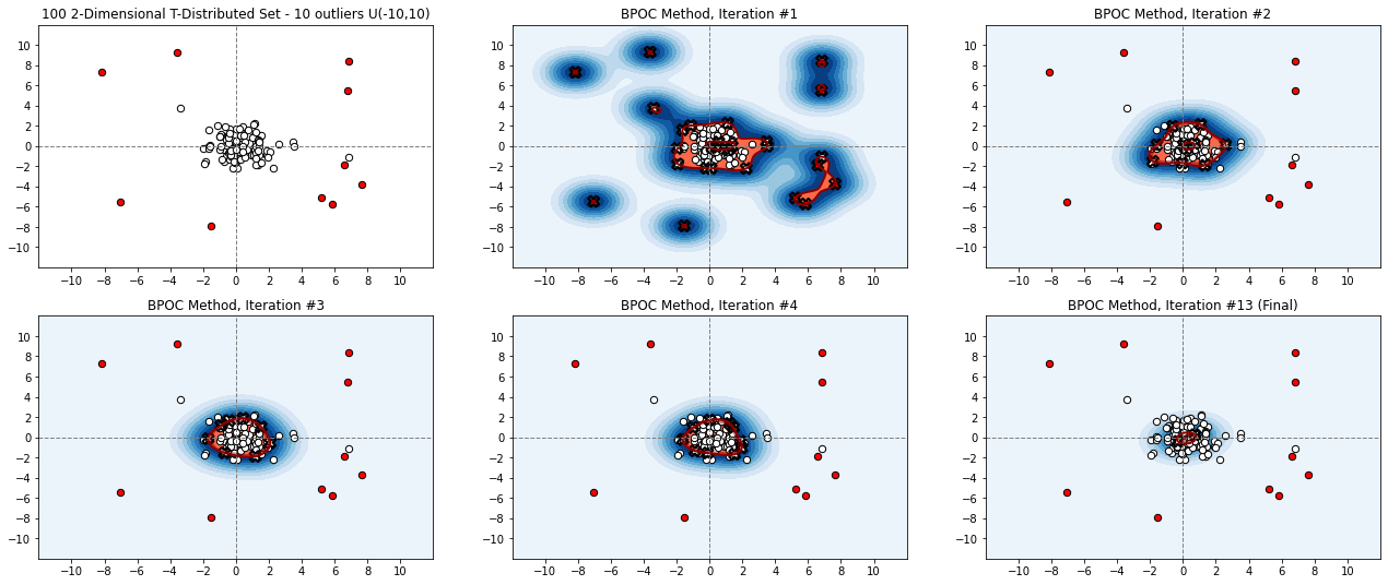
Figure 1: OCBP Example on a 2-dimensional unimodal data set. 100 inlier observations generated from $T(df=5)$, and 10 outlier observations generated from $U(-10,10)$. Contours indicate kernel signed distances from separating hyperplane. Blue contours indicate positive distances (darker blue indicates distance closer to zero), while red indicate negative distances. Support vectors are marked with an X.

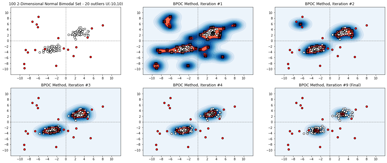
Figure 2: OCBP Example on a 2-dimensional bimodal data set. 50 inlier observations generated from $N(-3,1)$ and 50 inlier observations generated from $N(3,1)$. 20 outlier observations generated from $U(-10,10)$. Contours indicate kernel signed distances from separating hyperplane. Blue contours indicate positive distances (darker blue indicates distance closer to zero), while red indicate negative distances. Support vectors are marked with an X.

II-A Ensembled Boundary Peeling

To increase the sensitivity of the OCBP method, we computed the average distance calculated after fitting the OCBP method on feature sampled data, say $Y_{r}$. We call this approach the ensemble OCBP (EOCBP). While the OCBP algorithm Algorithm is relatively fast compared to other methods (see Table VII), the EOCBP algorithm is slower, but still a relatively strong-performing and feasible algorithm. The additional set of steps of the EOCBP algorithm is most prominent in line 5 of Algorithm Algorithm, where a subset of $\sqrt{p}$ of features are selected and the algorithm is iterated $c$ times. In our implementation we chose $c=50$ to limit the computational time in simulations. EOCBP flags outliers using and average of $\text{KDS}_{i}=d_{i}*\overline{f(x)}_{i}$ from each of the $c$ ensembles compared to a robust threshold, $h$, computed from the $\text{KDS}_{i}$ averaged over all $c$ iterations.

Algorithm The Ensemble OCBP Method

1:procedure EOCBP($S,q=0.01,n=2,c=50$)

2:     $r\leftarrow N$

3:     $S_{r}\leftarrow S$

4:     for $i\leftarrow 1$ to $c$ do

5:         $Y_{r}\leftarrow\text{colsample}(S_{r},int(\sqrt{p}))$

6:         while $r>n$ do

7:              $X_{SV}\leftarrow\text{OCSVM}(Y_{r},q,s)$

8:              $Y_{r}\leftarrow Y_{r}\char 92\relax X_{SV}$

9:              $D_{r}\leftarrow f(S)$

10:              $r\leftarrow\text{rows}(Y_{r})$

11:              $peel\leftarrow$ $peel+1$

12:              $depth_{i}\leftarrow$ $peel$

13:         end while

14:         $\text{d}\leftarrow$ $depth_{i}/peel$

15:         $\text{KDS}_{i}\leftarrow\text{mean}(D_{r})$

16:     end for

17:     $\text{EKDS}_{i}\leftarrow\text{mean}(\text{KDS}_{i})\times\text{mean}(d)$

18:     $h=Q_{3}\mathbf{(\text{EKDS})}+1.5\cdot\text{IQR}\mathbf{(\text{EKDS})}$

19:     $\text{flag}_{\text{EOCBP}}\leftarrow I(\text{ERKD}_{i}>h)$

20:     return $\text{ERKD}_{i},\text{flag}_{\text{EOCBP}}$

21:end procedure

III Synthetic Data Comparison

To explore the behavior of the OCBP and EOCBP methods under controlled circumstances, we conducted simulations of 1,000 data sets of size $n=50$, and dimension $p=100$ with sample observations drawn from the multivariate normal, T($df=5$), Lognormal and Wishart distributions on unimodal and multimodal data. For each of 1000 iterations we randomly generated sample data with different correlation structures; none, medium and high for data with no outliers and data with 10% outliers. For unimodal data with a single mode, data was generated with a $p$-dimensional mean vector $\bm{\mu}=\mathbf{0}$. For bimodal data the second mode has mean vector $\bm{\mu}=\mathbf{2}$ or $\bm{\mu}=\mathbf{5}$. When the data has no correlation $\Sigma=I$. For moderate or high correlation the off-diagonal elements of $\Sigma$ are equal to 0.5 or 0.75 respectively. Outliers for the Normal, T, and Wishart distributions are generated uniformly using $U(-10,10)$. For the lognormal distribution the outliers are generated using $U(-20,20)$. There is also a mixed distribution case where the correlation and distributions of each mode are chosen at random between 0, 0,5 and 0.75 and from the three distributions.

For a more realistic scenario we also conduct a simulation where the number modes, the distribution of the modes, the means and covariance of the modes, and percentage of outliers were randomly generated for each iteration. For each iteration $N$ was chosen randomly from $[50,150]$ and $p$ from [50,300]. In each case the number of modes was randomly selected from 1 to 5 where $N$ was divided equally among the number of modes. The off-diagonal elements of $\Sigma$ were chosen uniformly between 0 and 1. For each mode the data was randomly generated from the multivariate normal, T($df=5$), Lognormal and Wishart distributions. The percentage of contamination randomly selected between three different settings that include no contamination, 1 to 10% and 10 to 20%. The outlying observations were generated from the $U(-20,20)$ distribution.

For all scenarios we compare OCBP and EOCBP with ISO, ECOD, KNN, LOF, LUN, VAE and DSVDD. We implement each method using the default/recommended settings listed in the PYOD package [28] and the OCBP and EOCBP parameters as shown in Algorithms 1 and 2. The contamination ratio ($cr$) is kept at a default value of 10% for all competing algorithms.

We measure performance using detection rate (DR), correct classification rate (CC), area under the curve, and precision. Using the usual measures of True Positive (TP), True Negative (TN) False Positive (FP) and False Negative (FN) we define the detection rate as $DR_{i}=\frac{{TP_{i}}}{{TP_{i}+FN_{i}}}\times 100$. We define correct classification for a dataset $i$ as $\text{CC}_{i}=\frac{TP_{i}+TN_{i}}{N}\times 100$ and Precision (PREC) is defined as $\text{PREC}_{i}=\frac{TP_{i}}{TP_{i}+FP_{i}}\times 100$. The Area Under the Curve (AUC) of the Receiver Operating Characteristic curve measures the probability of correctly separating inlier and outliers. For brevity, only the tables for CC and AUC are shown. Tables for DR and PREC can be found in the supplementary materials.

TABLE I: Correct Classification rates for unimodal and bimodal simulated data with no outliers for $N=50$ and $d=100$. The parenthesis indicate the mean(s) of the mode ($\mu_{0}$) or modes ($\bm{\mu}_{1},\bm{\mu}_{5}$).

	Cor	OCBP	EOCBP	ISO	ECOD	LOF	KNN	DSVDD	LUNAR	VAE
N(0)	0	100.00	94.856	99.824	90.000	90.000	90.002	90.000	90.000	90.000
LN(0)	0	98.284	95.890	99.996	90.000	90.000	90.000	90.000	90.000	90.000
T(0)	0	99.948	99.539	90.339	90.000	90.000	90.000	90.000	90.000	90.000
W(0)	0	100.00	98.730	99.794	90.000	90.000	90.000	90.000	90.000	90.000
N(0)	0.5	94.928	84.242	89.950	90.000	90.000	90.010	90.000	90.000	90.000
LN(0)	0.5	100.00	83.720	88.864	90.000	90.000	90.000	90.000	90.000	90.000
T(0)	0.5	99.440	95.979	88.238	90.000	90.000	90.003	90.000	90.000	90.000
W(0)	0.5	100.00	98.785	99.800	90.000	90.000	90.000	90.000	90.000	90.000
N(0)	0.75	88.778	83.932	86.430	90.000	90.000	90.034	90.000	90.000	90.000
LN(0)	0.75	82.641	90.742	87.104	90.000	90.000	90.000	90.000	90.000	90.000
T(0)	0.75	92.414	90.830	86.790	90.000	90.000	90.009	90.000	90.000	90.000
W(0)	0.75	100.00	98.788	99.803	90.000	90.000	90.001	90.000	90.000	90.000
N(0,5)	0	99.994	96.981	98.433	90.000	90.000	90.740	90.000	90.000	90.000
LN(0,5)	0	99.912	96.742	99.942	90.000	90.000	90.000	90.000	90.000	90.000
T(0,5)	0	100.00	86.444	88.492	90.000	90.000	90.009	90.000	90.000	90.000
W(0,5)	0	100.00	98.022	99.686	90.000	90.000	90.006	90.000	90.000	90.000
N(0,5)	0.5	99.238	87.376	86.536	90.000	90.000	90.002	90.000	90.000	90.000
LN(0,5)	0.5	100.00	86.880	87.834	90.000	90.000	90.001	90.000	90.000	90.000
T(0,5)	0.5	100.00	86.146	85.966	90.000	90.000	90.003	90.000	90.000	90.000
W(0,5)	0.5	100.00	98.060	99.696	90.000	90.000	90.001	90.000	90.000	90.000
N(0,5)	0.75	94.954	86.470	82.316	90.000	90.000	90.033	90.000	90.000	90.000
LN(0,5)	0.75	100.00	84.856	85.190	90.000	90.000	90.000	90.000	90.000	90.000
T(0,5)	0.75	99.752	86.108	84.618	90.000	90.000	90.004	90.000	90.000	90.000
W(0,5)	0.75	100.00	98.120	99.712	90.000	90.000	90.000	90.000	90.000	90.000

The results in Table I show when no outliers are present OCBP will have the best, most consistent, correct classification rate. This is the case for unimodal and bimodal data with two modes ($\bm{\mu}_{1}=0$ and $\bm{\mu}_{2}=5$). For small samples, this property is a protection against data loss. Note that for the many of the methods, the necessity of having to provide a percentage of outliers ahead of time forces the identification of 10% of points as outliers.

TABLE II: Correct Classification rates for unimodal and bimodal simulated data with 10% outliers for $N=50$ and $d=100$. The parenthesis indicate the mean(s) of the mode ($\mu_{0}$) or modes ($\bm{\mu}_{1},\bm{\mu}_{5}$).

	Cor	OCBP	EOCBP	ISO	ECOD	LOF	KNN	DSVDD	LUN	VAE
N(0)	0	100.00	99.793	100.00	93.333	88.367	93.167	79.440	93.333	93.333
N(0,5)	0	99.111	98.909	100.00	99.178	99.262	99.476	83.455	98.953	98.965
LN(0)	0	99.357	99.887	100.00	93.333	88.133	93.160	79.360	93.333	93.333
LN(0,5)	0	98.348	99.922	100.00	88.580	87.660	93.120	76.843	93.327	93.475
T(0)	0	99.263	97.837	99.757	93.320	88.253	93.147	79.200	93.333	93.333
T(0,5)	0	98.338	98.538	99.752	89.478	88.250	93.103	77.167	93.327	93.285
W(0)	0	99.867	99.867	100.00	93.333	88.700	92.967	76.600	93.333	93.333
W(0,5)	0	99.498	99.995	100.00	89.482	88.300	92.862	76.590	93.333	93.347
N(0)	0.5	99.757	97.717	99.993	93.320	87.880	92.863	80.033	93.333	93.333
N(0,5)	0.5	95.180	93.085	99.885	98.991	99.244	99.385	83.938	99.065	99.073
LN(0)	0.5	98.100	86.653	99.647	93.333	86.463	92.717	80.887	93.327	93.327
LN(0,5)	0.5	97.658	84.512	99.825	88.493	89.813	93.193	78.273	93.297	93.457
T(0)	0.5	99.237	97.393	99.430	93.093	87.373	92.517	80.067	93.307	93.300
T(0,5)	0.5	98.610	97.940	99.475	86.848	88.107	92.633	77.177	93.333	93.062
W(0)	0.5	99.800	100.00	100.00	93.333	88.767	92.900	76.667	93.333	93.333
W(0,5)	0.5	100.00	100.00	100.00	88.767	88.367	92.767	76.400	93.333	93.533
N(0)	0.75	99.867	97.517	99.897	93.167	87.057	92.707	84.093	93.333	93.333
N(0,5)	0.75	95.751	91.698	99.425	98.442	99.253	99.316	84.585	99.073	99.024
LN(0)	0.75	97.720	86.343	99.147	93.300	85.030	92.440	83.153	93.287	93.273
LN(0,5)	0.75	97.190	90.415	99.503	88.428	90.532	93.193	79.213	93.253	93.417
T(0)	0.75	99.257	97.110	99.100	92.520	86.930	92.503	83.033	93.333	93.333
T(0,5)	0.75	98.478	97.688	99.158	84.060	88.665	92.522	78.083	93.317	92.828
W(0)	0.75	99.867	99.933	100.00	93.333	88.867	92.900	77.200	93.333	93.333
W(0,5)	0.75	100.00	100.00	100.00	88.867	88.767	92.833	76.867	93.333	93.500
Mixed(0,5)		93.920	98.243	94.297	87.810	88.380	89.703	78.227	89.873	89.967
Average		98.507	96.300	99.512	91.784	89.502	93.539	79.463	93.892	93.896

TABLE III: AUC for unimodal and bimodal simulated data with no outliers for $N=50$ and $d=100$. The parenthesis indicate the mean(s) of the mode ($\mu_{0}$) or modes ($\bm{\mu}_{1},\bm{\mu}_{5}$).

	Cor	OCBP	EOCBP	ISO	ECOD	LOF	KNN	DSVDD	LUN	VAE
N(0)	0	100.00	100.00	100.00	100.00	100.00	100.00	46.798	99.736	99.652
N(0,5)	0	100.00	100.00	100.00	100.00	100.00	100.00	31.707	99.573	100.00
LN(0)	0	100.00	100.00	100.00	100.00	100.00	100.00	49.665	99.822	99.734
LN(0,5)	0	99.984	100.00	100.00	100.00	99.996	99.996	27.119	99.804	100.00
T(0)	0	99.998	99.999	99.994	99.992	99.998	99.998	51.463	99.676	99.668
T(0,5)	0	99.989	99.950	99.950	99.986	99.988	99.988	36.929	99.700	99.945
W(0)	0	100.00	100.00	100.00	100.00	100.00	100.00	30.444	99.400	98.656
W(0,5)	0	100.00	100.00	100.00	100.00	100.00	100.00	30.347	99.036	99.981
N(0)	0.5	100.00	100.00	100.00	99.994	100.00	100.00	47.930	99.978	99.979
N(0,5)	0.5	100.00	100.00	100.00	99.973	100.00	100.00	38.245	99.844	100.00
LN(0)	0.5	99.991	99.900	99.999	100.00	99.996	99.991	63.800	99.881	99.811
LN(0,5)	0.5	99.813	98.789	98.789	99.961	99.998	99.975	43.632	99.827	99.978
T(0)	0.5	99.977	99.970	99.960	99.844	99.984	99.977	51.867	99.737	99.747
T(0,5)	0.5	99.991	99.899	99.899	97.589	99.998	100.00	45.483	99.869	99.820
W(0)	0.5	100.00	100.00	100.00	100.00	100.00	100.00	29.668	98.548	99.024
W(0,5)	0.5	100.00	100.00	100.00	100.00	100.00	100.00	26.775	99.363	100.00
N(0)	0.75	100.00	100.00	100.00	99.892	100.00	100.00	63.888	99.990	99.987
N(0,5)	0.75	100.00	100.00	100.00	99.696	100.00	100.00	49.808	99.953	100.00
LN(0)	0.75	99.946	99.535	99.969	99.979	99.987	99.943	73.388	99.872	99.853
LN(0,5)	0.75	99.668	98.252	98.252	99.759	99.987	99.956	53.806	99.811	99.942
T(0)	0.75	99.998	99.992	99.977	99.504	99.998	99.999	64.051	99.908	99.956
T(0,5)	0.75	99.990	99.859	99.859	94.978	99.992	99.994	49.713	99.908	99.686
W(0)	0.75	100.00	100.00	100.00	100.00	100.00	100.00	31.076	99.040	98.552
W(0,5)	0.75	100.00	100.00	100.00	100.00	100.00	100.00	28.714	98.592	100.00
Mixed(0,5)		99.880	99.884	99.884	98.818	99.944	99.920	67.938	99.806	99.939
Average		99.968	99.834	99.855	99.582	99.994	99.989	45.311	99.622	99.761

.

Table II shows the CC rate for unimodal data with $\bm{\mu}=0$ and bimodal data with $\bm{\mu}_{1}=0$ and $\bm{\mu}_{2}=5$. ISO has the highest CC for most levels of correlation and distribution, closely followed by OCBP for the zero correlation case. For moderate correlation OCBP, EOCBP and ISO all have a perfect CC for the bimodal Wishart distribution case and EOCBP and ISO for the unimodal case. LOF produces the second highest CC for the bimodal moderately correlated Normal data. When the correlation is high we observe that OCBP and EPOC methods fair the best when the data is non-normal. In general we do not observe a difference between unimodal and bimodal data in terms of CC. We do observe that EOCBP has a slightly lower CC for highly-correlated lognormal data. When the correlation and distribution of the two modes is mixed, EOCBP has the highest CC rate. Overall ISO produces the highest average CC followed by OCBP then EOCBP. DSVDD had the lowest average CC overall.

Table III shows that all of the methods except for DSVDD have high values of AUC indicating that, at some cut off value, each method will be able to almost perfectly identify outliers in this simulated data. LOF has the highest overall average AUC followed by KNN then OCBP then VAE. ISO and EOCBP have the same same performance in the mixed distribution case, closely followed by OCBP.

Although not shown in the main body of the paper, the DR is high for most methods and for many cases (see Supplementary Materials). Data with two normally distributed modes, regardless of correlation structure, leads to the highest DR. ISO has the has a perfect DR except for the mixed distributions. For every case where ISO has a DR of 100% OCBP or EOCBP either also have a DR of 100% or have a DR of 99.272% or higher. EOCBP has the highest DR for the case when the modes have random distributions. ISO has the highest average DR=99.493 overall followed by OCBP=99.469 in close second. DSVDD has the lowest DR overall. ISO has the highest average precision followed by VAE, LUN and KNN (see Supplementary Materials). Interestingly, several of the methods, including OCBP and EOCBP have prefect precision when the modes are generated from the Wishart distribution and the correlation is high. In general a method that has a lower precision but a high detection rate is tending to flag more inliers as outliers.

Table IV gives the result of the random simulation. When no outliers are present, OCBP has the highest CC followed by EOCBP. This is also the case when outliers are present between 1% and 10%. At the the higher percentage of outliers, ISO has the best CC followed by LOF. When data contain 1-10% outliers ISO, LOF, KNN, LUN and VAE all have a DR=100.00%. For the higher percentage of outliers only KNN has a DR=100.00%. OCBP and EOCBP have a mid level DR at 98.208 and 98.734 respectively. This performance is consistent with what we have observed with OCBP and EOCBP of identifying less observations as outliers overall. This conservative behaviour is reflected in the high Precision observed in Table IV with both measures having the highest precision. Many of the measures have an extremely high AUC, EOCBP having the highest for a outliers between 1 and 10% and KNN having the highest overall. EOCBP has the second highest AUC whereas ECOD and DVSVDD have the lowest AUC.

TABLE IV: Summary of measures for each method on data with a randomly generated number of modes from random distributions and random correlation structure. Bold indicates the best performance.

Measure	% Out	OCBP	EOCBP	ISO	ECOD	LOF	KNN	DVSDD	LUN	VAE
CC	none	97.878	94.050	87.986	89.645	91.243	91.015	89.650	89.650	89.650
	1 to 10	99.040	96.881	93.504	90.395	93.078	92.743	88.392	91.559	91.559
	10 to 20	96.401	94.502	97.035	91.060	96.646	96.505	85.982	95.499	95.482
DR	1 to 10	99.803	99.608	100.00	99.350	100.00	100.00	98.233	100.00	100.00
	10 to 20	98.208	98.734	99.998	97.455	99.950	100.000	94.614	99.927	99.917
PREC	1 to 10	99.211	97.233	93.456	90.822	92.967	92.622	89.789	91.422	91.422
	10 to 20	98.076	95.505	96.879	92.941	96.524	96.326	90.214	95.334	95.325
AUC	1 to 10	99.680	99.966	99.934	83.660	99.850	99.978	48.067	99.574	99.701
	10 to 20	99.662	99.972	99.934	83.574	99.839	99.983	53.324	99.639	99.552

IV Example Data Comparison

[36] utilized semantically meaningful datasets to evaluate multiple outlier detection methods. The original datasets include a labeled class that can be assumed to be rare and therefore outliers. For example, a class of sick patients within a population dominated by healthy patients. The prepared datasets are from benchmark data commonly used in the outlier literature [36]. To prepare the datasets, the authors sampled (where possible) the outlying class at different rates 20%, 10%, 5%, and 2%. Because the datasets were sampled, to avoid bias, 10 different versions for each percentage of outliers for each data set were created. Note that not every dataset was created with all four different percentages of outliers due to the amount of observations in the outlier class. The authors give versions of these sample datasets that are normalized to [0,1] and with duplicates removed and non-normalized versions that contain duplicate observations. To emulate the most realistic scenario where data pre-processing has taken place we use the normalized datasets with no duplicates for a total of 1700 datasets. The datasets are available here: https://www.dbs.ifi.lmu.de/research/outlier-evaluation/ and the attribute type and number and sample size of each original dataset is summarized in Table LABEL:tab:semantic_data. Regarding the shape of the data, there no way to tell if this data is multi-modal, but several of the datasets contain data that belongs to more than two classes and therefore it might be reasonable to assume that some of these datasets might contain more than a single mode.

Table V shows the average CC across all versions of the datasets. This includes datasets with 2-20% outliers. EOCBP has the highest CC in 7 of the 11 datasets with ISO having a 1 of the highest and KNN having 3 of the highest.

Table VI shows the average AUC across all versions of the data. EOCBP has the highest average AUC in 5 cases where ISO has the highest AUC in 4 cases. OCBP has the highest average AUC for two cases. Since AUC is independent of the specific choice of cutoff indicating the EBOPC method is better at separating the outliers from the inliers for these datasets.

Although not shown in the main body of the paper, the DR is sporadic across the methods and the datasets with ISO and OCBP having 3 and 4 of the top DR respectively. In general the DR for these datasets are low and variable. For example for the Hepatitis data ISO had a detection rate of 85% whereas OCBP had a detection rate of 0. Likewise ISO has a 0% detection rate for the InternetAds data whereas LOF has 55% DR.

In 5 out the 8 datasets EOCBP has the highest precision. In two cases OCBP has a precision of 0% and in one case ISO hasa a precision of 0%. Lastly Table VII shows the average processing time overall versions of each of the datasets. OCBP had four of the fastest processing times but KNN had the overall average fastest processing time. Processing times were measured in seconds using a workstation with an Intel Xeon Processor E5-2687W and dual SLI NVIDIA Quadro P5000 graphical processing units (GPU).

TABLE V: Average correct classification rate overall of the semantically created normalized data sets without duplicates for each outlier detection method.

Data	OCBP	EOCBP	ISO	ECOD	LOF	KNN	DSVD	LUN	VAE
Annthyroid	86.270	94.730	93.350	88.860	88.500	87.950	89.090	87.970	87.490
Arrhythmia	84.900	91.410	91.940	90.930	87.110	87.540	83.820	87.240	86.970
Cardiotocography	84.090	89.770	87.070	87.330	84.920	85.890	83.630	85.180	86.670
HeartDisease	83.930	91.210	70.300	86.740	83.140	85.330	84.070	84.050	86.700
Hepatitis	93.130	91.380	60.820	85.890	86.580	84.930	84.500	88.230	88.360
InternetAds	94.360	94.820	94.360	94.260	89.980	91.060	88.400	89.490	89.730
PageBlock	84.310	87.040	89.770	90.700	90.290	90.790	88.840	90.620	90.880
Parkinson	86.120	87.340	85.910	85.930	87.750	88.320	82.980	87.280	87.410
Pima	80.900	85.790	82.980	85.050	83.610	84.500	82.050	84.730	84.470
SpamBas	84.720	90.170	90.290	85.930	83.070	84.570	83.600	84.780	84.740
Stamps	85.550	87.160	89.810	89.640	88.050	89.890	87.480	89.640	89.450
Average	86.207	90.075	85.145	88.296	86.636	87.343	85.315	87.201	87.534

TABLE VI: Average AUC rate overall of the semantically created normalized data sets without duplicates for each outlier detection methods.

Data	OCBP	EOCBP	ISO	ECOD	LOF	KNN	DSVD	LUN	VAE
Annthyroid	50.363	64.337	67.155	23.172	31.940	35.286	27.580	35.114	39.604
Arrhythmia	77.280	77.316	77.590	22.040	22.796	22.106	46.367	24.545	22.945
Cardiotocography	78.540	79.396	75.904	17.123	31.430	33.466	49.347	35.359	20.667
HeartDisease	77.012	84.692	80.960	20.377	30.105	23.889	35.427	29.932	20.372
Hepatitis	74.534	78.077	76.269	21.311	21.876	26.162	41.400	19.140	18.927
InternetAds	70.416	68.690	62.374	28.626	24.682	18.690	27.871	20.554	21.348
PageBlock	91.307	86.824	91.220	7.127	17.687	10.300	41.468	11.858	8.020
Parkinson	74.233	80.435	81.938	24.931	23.369	15.990	40.631	14.106	27.150
Pima	69.655	72.148	71.725	33.170	33.357	26.524	50.383	28.447	30.130
SpamBase	67.949	77.375	77.054	24.213	31.658	27.813	42.403	27.880	28.258
Stamps	88.311	91.302	91.731	9.173	12.096	8.252	38.641	13.405	8.406
Average	74.509	78.236	77.629	21.024	25.545	22.589	40.138	23.667	22.348

TABLE VII: Average processing time in seconds for normalized data sets without duplicates processing times were measured in seconds using a workstation with an Intel Xeon Processor E5-2687W and dual SLI NVIDIA Quadro P5000 graphical processing units (GPU).

Data	OCBP	EOCBP	ISO	ECOD	LOF	KNN	DSVD	LUN	VAE
Annthyroid	11.475	1026.208	0.431	5.972	1.130	1.126	14.370	3.785	26.004
Arrhythmia	0.119	3.346	0.277	0.043	0.159	0.160	2.404	2.543	4.946
Cardiotocography	0.821	99.658	0.316	0.262	0.382	0.382	5.627	3.660	150.287
HeartDisease	0.017	3.208	0.263	0.020	0.037	0.035	2.237	1.661	3.434
Hepatitis	0.008	0.973	0.258	0.021	0.220	0.220	1.973	3.054	2.835
InternetAds	7.325	155.107	1.780	1.036	0.478	0.688	10.339	4.824	925.483
PageBlock	6.243	1379.576	0.383	3.662	0.116	0.179	10.945	3.038	16.824
Parkinson	0.007	0.417	0.257	0.032	0.221	0.222	2.601	2.699	3.039
Pima	0.094	15.080	0.281	0.143	27.987	0.037	3.042	1.677	4.810
SpamBase	1.913	245.913	0.359	1.169	0.598	0.621	7.002	4.084	14.090
Stamps	0.066	7.804	0.268	0.015	0.038	0.035	2.542	1.700	3.758
Average	2.553	267.026	0.443	1.125	2.851	0.337	5.735	2.975	105.046

In the implementation of the methods in the PyOD package, the users must specify the percentage of outliers in the data. We set that to be 10% for all of the methods. We show the DR, CC, AUC and Precision for only the sampled datasets with 10% outliers. Generally we see similar patterns as before. DR is fairly sporadic with OCBP having three of the highest values. EOCBP dominates correct classification for the datasets with only 10% outliers. EOCBP had four of the highest AUC values followed by ISO with three of the highest values. ISO shows a precision of 100% for the Arrhythmia datasets with 10% outliers, however, EOCBP has four of the highest precision values for the remainder of the datasets.

V Discussion

We have introduced a novel method for outlier detection based on iteratively peeled observations and signed distances. We have compared our method with state-of-the art methods on unimdoal and multimodal synthetic and on semantically meaningful benchmark data. From the synthetic data studies we can make the following conclusions. When no outliers are present OCBP has a higher CC rate than ISO in all but a single case. All methods have high CC and DR rates for unimodal and bimodal data with 10% outliers, OCBP and EOCBP included. LOF has the highest average AUC for all synthetic data with OCBP with the second highest. . In the case of completely randomly generated synthetic data OCBP has the highest CC rate for data with 0-10% outliers and the highest precision. KNN has the highest AUC but OCBP and EOCBP are on par with AUCs of all of the other methods.

From the synthetic data comparison we conclude that the performance of OCBP and EOCBP will be equivalent when outliers are present and better if there are no outliers present. For small sample data, preventing unnecessary data loss by eliminating inliers is potentially a problem. Using OCBP or EOCBP will protect against unessary data loss in the case of a small sample.

The comparison of the methods on the semantically created benchmark datasets illustrates the following. EOCBP had the highest overall CC but not the highest overall DR indicating it is conservative in its identification of outliers. The method with the highest average DR is ISO followed by closely by VAE. VAE never had the highest DR for a single dataset, but had the most consistent performance. Although EOCBP did not have highest DR it did have the highest AUC and Precision. This indicates that the default threshold for outlier identification might not be optimal. The most consistent, computationally, efficient method is KNN. In its current implementation, EOCBP is the least efficient. However OCBP is about average compared to the other methods. We can conclude that EOCBP is performs better on a variety of data types. Further work is required to increase the computational efficiency of the method. If computational efficiency is necessary, the OCBP method will perform equivalently to the other methods.

One weakness of the OCBP and EOCBP involves the size of the modes. In the synthetic data random mode simulation the modes created had different sizes, but not despairingly different. If one mode contained almost all of the data and another was small, OCBP and EOCBP would probably categorize the observations in the smaller mode as outliers. We tested the performance of the OCBP and EOCBP against the other algorithms and although the performance in terms of the correct classification rate is lower compared to cases where the number of modes is similar, they perform competitively and most often outperform competing methods.

OCBP and EOCBP were implemented with baseline parameters and the performance of both could be improved by tuning, specifically the value $h$ the outlier threshold and further research is warranted here since OCBP proves to be a computationally efficient method (see Table VII). In the implementation of EOCBP, the parameter $c$ and the feature set, $\sqrt{p}$ were set to strict values. Changing these might improve the computational efficiency and sensitivity of the method.

For both methods the boundaries created by OCSVM were set to be as large as possible and hence peel a small number of observations at a time. For a dataset with a large number of observations, adjusting $q$ so that smaller boundaries are created each peel would improve the computational efficiency by requiring fewer peels.

References

- [1] A. Westerski, R. Kanagasabai, E. Shaham, A. Narayanan, J. Wong, and M. Singh, “Explainable anomaly detection for procurement fraud identification—lessons from practical deployments,” International Transactions in Operational Research, vol. 28, no. 6, pp. 3276–3302, 2021.
- [2] H. Zhang, W. Guo, S. Zhang, H. Lu, and X. Zhao, “Unsupervised deep anomaly detection for medical images using an improved adversarial autoencoder,” Journal of Digital Imaging, vol. 35, no. 2, pp. 153–161, 2022.
- [3] A. Ponmalar and V. Dhanakoti, “An intrusion detection approach using ensemble support vector machine based chaos game optimization algorithm in big data platform,” Applied Soft Computing, vol. 116, p. 108295, 2022.
- [4] C. C. Aggarwal and C. C. Aggarwal, An introduction to outlier analysis. Springer, 2017.
- [5] R. Domingues, M. Filippone, P. Michiardi, and J. Zouaoui, “A comparative evaluation of outlier detection algorithms: Experiments and analyses,” Pattern recognition, vol. 74, pp. 406–421, 2018.
- [6] X. Tan, J. Yang, and S. Rahardja, “Sparse random projection isolation forest for outlier detection,” Pattern Recognition Letters, vol. 163, pp. 65–73, 2022.
- [7] B. Schölkopf, J. C. Platt, J. Shawe-Taylor, A. J. Smola, and R. C. Williamson, “Estimating the support of a high-dimensional distribution,” Neural computation, vol. 13, no. 7, pp. 1443–1471, 2001.
- [8] P. Filzmoser, R. Maronna, and M. Werner, “Outlier identification in high dimensions,” Computational statistics & data analysis, vol. 52, no. 3, pp. 1694–1711, 2008.
- [9] S. Nedelkoski, J. Cardoso, and O. Kao, “Anomaly detection from system tracing data using multimodal deep learning,” in 2019 IEEE 12th International Conference on Cloud Computing (CLOUD), pp. 179–186, IEEE, 2019.
- [10] J. Sipple, “Interpretable, multidimensional, multimodal anomaly detection with negative sampling for detection of device failure,” in International Conference on Machine Learning, pp. 9016–9025, PMLR, 2020.
- [11] D. Park, Z. Erickson, T. Bhattacharjee, and C. C. Kemp, “Multimodal execution monitoring for anomaly detection during robot manipulation,” in 2016 IEEE International Conference on Robotics and Automation (ICRA), pp. 407–414, IEEE, 2016.
- [12] Y. Feng, Z. Liu, J. Chen, H. Lv, J. Wang, and X. Zhang, “Unsupervised multimodal anomaly detection with missing sources for liquid rocket engine,” IEEE Transactions on Neural Networks and Learning Systems, 2022.
- [13] D. Lahat, T. Adali, and C. Jutten, “Multimodal data fusion: an overview of methods, challenges, and prospects,” Proceedings of the IEEE, vol. 103, no. 9, pp. 1449–1477, 2015.
- [14] L. Chiang, B. Lu, and I. Castillo, “Big data analytics in chemical engineering,” Annual review of chemical and biomolecular engineering, vol. 8, pp. 63–85, 2017.
- [15] M. Quiñones-Grueiro, A. Prieto-Moreno, C. Verde, and O. Llanes-Santiago, “Data-driven monitoring of multimode continuous processes: A review,” Chemometrics and Intelligent Laboratory Systems, vol. 189, pp. 56–71, 2019.
- [16] F. T. Liu, K. M. Ting, and Z.-H. Zhou, “Isolation-based anomaly detection,” ACM Transactions on Knowledge Discovery from Data (TKDD), vol. 6, no. 1, pp. 1–39, 2012.
- [17] T. R. Bandaragoda, K. M. Ting, D. Albrecht, F. T. Liu, Y. Zhu, and J. R. Wells, “Isolation-based anomaly detection using nearest-neighbor ensembles,” Computational Intelligence, vol. 34, no. 4, pp. 968–998, 2018.
- [18] M. M. Breunig, H.-P. Kriegel, R. T. Ng, and J. Sander, “Lof: identifying density-based local outliers,” in ACM sigmod record, vol. 29, pp. 93–104, ACM, 2000.
- [19] S. Ramaswamy, R. Rastogi, and K. Shim, “Efficient algorithms for mining outliers from large data sets,” in ACM Sigmod Record, vol. 29, pp. 427–438, ACM, 2000.
- [20] A. Goodge, B. Hooi, S.-K. Ng, and W. S. Ng, “Lunar: Unifying local outlier detection methods via graph neural networks,” in Proceedings of the AAAI Conference on Artificial Intelligence, vol. 36, pp. 6737–6745, 2022.
- [21] J. Chen, S. Sathe, C. Aggarwal, and D. Turaga, “Outlier detection with autoencoder ensembles,” in Proceedings of the 2017 SIAM international conference on data mining, pp. 90–98, SIAM, 2017.
- [22] O. Lyudchik, “Outlier detection using autoencoders,” tech. rep., 2016.
- [23] C. Zhou and R. C. Paffenroth, “Anomaly detection with robust deep autoencoders,” in Proceedings of the 23rd ACM SIGKDD international conference on knowledge discovery and data mining, pp. 665–674, 2017.
- [24] Y. Liu, Z. Li, C. Zhou, Y. Jiang, J. Sun, M. Wang, and X. He, “Generative adversarial active learning for unsupervised outlier detection,” IEEE Transactions on Knowledge and Data Engineering, vol. 32, no. 8, pp. 1517–1528, 2019.
- [25] L. Ruff, R. Vandermeulen, N. Goernitz, L. Deecke, S. A. Siddiqui, A. Binder, E. Müller, and M. Kloft, “Deep one-class classification,” in International conference on machine learning, pp. 4393–4402, PMLR, 2018.
- [26] G. E. Hinton and R. R. Salakhutdinov, “Reducing the dimensionality of data with neural networks,” science, vol. 313, no. 5786, pp. 504–507, 2006.
- [27] D. P. Kingma and M. Welling, “Auto-encoding variational bayes,” arXiv preprint arXiv:1312.6114, 2013.
- [28] Y. Zhao, Z. Nasrullah, and Z. Li, “Pyod: A python toolbox for scalable outlier detection,” arXiv preprint arXiv:1901.01588, 2019.
- [29] Z. Li, Y. Zhao, X. Hu, N. Botta, C. Ionescu, and G. Chen, “Ecod: Unsupervised outlier detection using empirical cumulative distribution functions,” IEEE Transactions on Knowledge and Data Engineering, 2022.
- [30] W. G. Martinez, M. L. Weese, and L. A. Jones-Farmer, “A one-class peeling method for multivariate outlier detection with applications in phase i spc,” Quality and Reliability Engineering International, vol. 36, no. 4, pp. 1272–1295, 2020.
- [31] D. M. Tax and R. P. Duin, “Support vector domain description,” Pattern recognition letters, vol. 20, no. 11-13, pp. 1191–1199, 1999.
- [32] V. Barnett, “The ordering of multivariate data,” Journal of the Royal Statistical Society. Series A (General), pp. 318–355, 1976.
- [33] D. M. Tax and R. P. Duin, “Support vector data description,” Machine learning, vol. 54, no. 1, pp. 45–66, 2004.
- [34] A. Bounsiar and M. G. Madden, “One-class support vector machines revisited,” in 2014 International Conference on Information Science & Applications (ICISA), pp. 1–4, IEEE, 2014.
- [35] L. Lee, M. L. Weese, W. G. Martinez, and L. A. Jones-Farmer, “Robustness of the one-class peeling method to the gaussian kernel bandwidth,” Quality and Reliability Engineering International, vol. 38, no. 3, pp. 1289–1301, 2022.
- [36] G. O. Campos, A. Zimek, J. Sander, R. J. Campello, B. Micenková, E. Schubert, I. Assent, and M. E. Houle, “On the evaluation of unsupervised outlier detection: measures, datasets, and an empirical study,” Data Mining and Knowledge Discovery, vol. 30, no. 4, pp. 891–927, 2016.