Minimum Area Confidence Set Optimality for Simultaneous Confidence Bands for Percentiles in Linear Regression

Abstract

Simultaneous confidence bands (SCBs) for percentiles in linear regression are valuable tools with many applications. In this paper, we propose a novel criterion for comparing SCBs for percentiles, termed the Minimum Area Confidence Set (MACS) criterion. This criterion utilizes the area of the confidence set for the pivotal quantities, which are generated from the confidence set of the unknown parameters. Subsequently, we employ the MACS criterion to construct exact SCBs over any finite covariate intervals and to compare multiple SCBs of different forms. This approach can be used to determine the optimal SCBs.

It is discovered that the area of the confidence set for the pivotal quantities of an asymmetric SCB is uniformly and can be very substantially smaller than that of the corresponding symmetric SCB. Therefore, under the MACS criterion, exact asymmetric SCBs should always be preferred. Furthermore, a new computationally efficient method is proposed to calculate the critical constants of exact SCBs for percentiles. A real data example on drug stability study is provided for illustration.

Keywords: Simultaneous confidence band; Confidence sets; Minimum area; Linear regression; Percentile line.

1 Introduction

In this paper, we consider the simple linear regression model with mean-centred covariates,

$$y_{i}={\bm{x}}_{i}^{T}\bm{\beta}+\epsilon_{i}=\beta_{0}+\beta_{1}(x_{i}-\bar{x})+\epsilon_{i},\ i=1,2,\dots,n,$$

where $\bar{x}=\frac{1}{n}\sum_{i=1}^{n}x_{i}$, ${\bm{x}}_{i}=(1,x_{i}-\bar{x})^{T}$, $\bm{\beta}=(\beta_{0},\beta_{1})^{T}$, the random errors $\epsilon_{i}$ are identically and independently distributed as $N(0,\sigma^{2})$, and $\beta_{0}$, $\beta_{1}$ and $\sigma^{2}$ are unknown parameters. Let $\bm{X}$ denote the centered design matrix, the $i$th row of which is given by $\bm{x}_{i}^{T}$, $i=1,2,\dots,n$. Let $S_{xx}=\sum_{i=1}^{n}(x_{i}-\bar{x})^{2}$, then $(\bm{X}^{T}\bm{X})^{-1}$ is a $2\times 2$ diagonal matrix given by

$$(\bm{X}^{T}\bm{X})^{-1}=\begin{pmatrix}1/n&0\\ 0&1/S_{xx}\end{pmatrix}.$$ (1)

Denote the least square estimators of $\bm{\beta}$ and $\sigma^{2}$ by $\hat{\bm{\beta}}=(\hat{\beta}_{0},\hat{\beta}_{1})^{T}=(\bm{X}^{T}\bm{X})^{-1}\bm{X}\bm{y}$ and $\hat{\sigma}^{2}=\frac{(\bm{y}-\hat{\bm{y}})^{T}(\bm{y}-\hat{\bm{y}})}{\nu}$ with $\nu=n-2$, $\bm{y}=(y_{1},\dots,y_{n})^{T}$ and $\hat{\bm{y}}={\bm{x}}^{T}\hat{\bm{\beta}}$, respectively. Then, $\hat{\bm{\beta}}\sim N_{2}(\bm{\beta},\sigma^{2}(\bm{X}^{T}\bm{X})^{-1})$, $\hat{\sigma}/\sigma\sim\sqrt{\chi^{2}_{\nu}/\nu}$, and $\hat{\bm{\beta}}$ and $\hat{\sigma}$ are independent random variables.

1.1 Simultaneous Confidence Band for Percentiles in Linear Regression

For linear regression model, the general $100\gamma$th percentile regression line is

$$\bm{x}^{T}\bm{\beta}+z_{\gamma}\sigma,$$

where $z_{\gamma}$ is the $100\gamma$th percentile of the standard normal distribution, i.e., $\Phi(z_{\gamma})=\int_{-\infty}^{z_{\gamma}}\phi(x)dx=\gamma$ with $\phi(x)=\exp(-x^{2}/2)/\sqrt{2\pi}$. It is noteworthy that the mean regression line $\bm{x}^{T}\bm{\beta}$ is the 50th percentile, which is a special case of the percentile line $\bm{x}^{T}\bm{\beta}+z_{\gamma}\sigma$ with $\gamma=0.5$. Several articles, including Spurrier (1999), Al-Saidy et al. (2003), Liu et al. (2004, 2007, 2009) and Piegorsch et al. (2005), have studied simultaneous confidence bands (SCBs) for $\bm{x}^{T}\bm{\beta}$. SCBs for the $100\gamma$th percentile line $\bm{x}^{T}\bm{\beta}+z_{\gamma}\sigma$ over the whole covariate range $(-\infty,\infty)$, have been studied by Steinhorst and Bowden (1971), Turner and Bowden (1977, 1979) and Thomas and Thomas (1986). It is known that, linear regression models are often constructed for a finite covariate range, and an exact SCB over a finite interval $(a,b)$ can be substantially narrower than a conservative SCB which is constructed over the entire covariate range $(-\infty,\infty)$ in terms of average band width, and so exact SCBs are more informative. Han et al. (2015) has proposed a method for constructing exact asymmetric SCBs for percentiles over a finite interval $(a,b)$.

In this paper, we focus on the SCBs $(l(x),u(x))$ for the $100\gamma$th percentile line $\bm{x}^{T}\bm{\beta}+z_{\gamma}\sigma$, over a finite interval of interest $x-\bar{x}\in(a,b)$, that have confidence level equal to $1-\alpha$:

$$\inf_{-\infty<\beta_{0},\beta_{1}<\infty,\ \sigma>0}P\Bigl{\{}l(x)\leq\bm{x}^{T}\bm{\beta}+z_{\gamma}\sigma\leq u(x)\ \text{for all}\ x-\bar{x}\in(a,b)\Bigr{\}}=1-\alpha.$$ (2)

In drug stability studies, the $100\gamma$th percentile line can be more important than the mean regression line $\bm{x}^{T}\bm{\beta}$. In order to measure the degradation of active pharmaceutical ingredients over time, drug stability studies are commonly conducted in the pharmaceutical industry. For example, it is expected that drug content of a large proportion of dosage units, say $95\%$ of tablets, should be larger than the threshold $h$ (in percentage) before an expected expiry date. Hence, the percentile line with $\gamma=1-95\%=5\%$ is of interest. In this case, a two-sided SCB with a specific confidence level (e.g., $1-\alpha=95\%$) for the $5\%$-percentile line should be used to determine the expiry date.

Consider two-sided SCBs of the form

$$\bm{x}^{T}\hat{\bm{\beta}}+z_{\gamma}\hat{\sigma}/\theta- c_{1}\hat{\sigma}\sqrt{\bm{x}^{T}(\bm{X}^{T}\bm{X})^{-1}\bm{x}+(z_{\gamma})^{2}\xi}\leq\bm{x}^{T}\bm{\beta}+z_{\gamma}\sigma$$

$$\leq\bm{x}^{T}\hat{\bm{\beta}}+z_{\gamma}\hat{\sigma}/\theta+c_{2}\hat{\sigma}\sqrt{\bm{x}^{T}(\bm{X}^{T}\bm{X})^{-1}\bm{x}+(z_{\gamma})^{2}\xi}\qquad\text{for all}\ x-\bar{x}\in(a,b),$$ (3)

where $c_{1}$ and $c_{2}$ denote the critical constants satisfy $(\ref{condition})$, and the constants $\theta\neq 0$ and $\xi$ are selected for constructing different forms of SCBs. The symmetric SCB, with $c_{1}=c_{2}=c$, is a special case of SCBs in (3). In this paper, we consider six different forms of SCBs, which are the only forms available in the literature; see Steinhorst and Bowden (1971), Turner and Bowden (1977), Thomas and Thomas (1986), and Han et al. (2015). Table 1 gives the values of $\xi$ and $\theta$ for these six bands: SB, TBU and TBE (Type $I$ with $\xi=0$), V, UV and TT (Type $II$ with $\xi\neq 0$). The corresponding asymmetric bands are denoted as SBa, TBUa, TBEa, Va, UVa and TTa, respectively.

Table 1: Six simultaneous confidence bands

Name	Type	$\xi$	$\theta$	Origin
SB	$I$	0	1	Steinhorst and Bowden (1971)
TBU	$I$	0	$\sqrt{\frac{2}{v}}\frac{\Gamma(\frac{v+1}{2})}{\Gamma(\frac{v}{2})}$	Turner and Bowden (1977)
TBE	$I$	0	$\sqrt{\frac{2}{v}}\frac{\Gamma(\frac{v}{2})}{\Gamma(\frac{v-1}{2})}$	Turner and Bowden (1977)
V	$II$	$1-\frac{2}{v}\Big{(}\frac{\Gamma(\frac{v+1}{2})}{\Gamma(\frac{v}{2})}\Big{)}^{2}$	1	Han et al. (2015)
UV	$II$	$\frac{v}{2}\Big{(}\frac{\Gamma(\frac{v+1}{2})}{\Gamma(\frac{v}{2})}\Big{)}^{2}-1$	$\sqrt{\frac{2}{v}}\frac{\Gamma(\frac{v+1}{2})}{\Gamma(\frac{v}{2})}$	Han et al. (2015)
TT	$II$	$\frac{1}{2v}$	$\frac{4v-1}{4v}$	Thomas and Thomas (1986)

The pursuit of an optimal SCB is motivated by the desire to identify the most informative SCB among the different available forms given above. The average width (AW) of a SCB has been widely used as an optimality criterion for comparing different forms of confidence bands since Gafarian (1964). In the context of percentiles of linear regression, Han et al. (2015) has conducted a thorough comparison of SCBs under the AW criterion. However, one drawback of the AW criterion, as pointed out in Liu and Hayter (2007), is that it may give too much weight to the interval of interest $(a,b)$ on which the confidence band is presented. Hence, we consider the comparison under the minimum area confidence set (MACS) criterion. Several authors have studied optimal confidence bands for the mean regression line, $\bm{x}^{T}\bm{\beta}$, using the MACS criterion based on the confidence set of $\bm{\beta}$ only; see Liu and Hayter (2007), Liu et al. (2008), and Liu and Ah-kine (2010). Liu and Hayter (2007) has employed the MACS criterion to compare simultaneous confidence bands (SCBs) in the context of simple linear regression, and identified the optimal SCB for various scenarios. Additionally, Liu and Ah-kine (2010) focuses on finding the best inner-hyperbolic band for the simple linear regression model utilising the MACS criterion. In this paper, we construct pivotal quantities that are generated from the unknown parameters $(\bm{\beta},\sigma)$ via a linear transformation. The area of the confidence set of the pivotal quantities is used as the new MACS criterion, and we aim to find the optimal SCBs that minimise the area of corresponding confidence set. Since the comparison of SCBs for percentiles in the linear regression has not been conducted under the MACS criterion, this paper aims to fill this gap. We also propose an efficient method to calculate critical constants of SCBs for percentiles, and this method can significantly reduce computational costs.

The layout of the paper is as follows. Section 2 considers the construction of confidence sets for several SCBs for percentile line, including Type $I$ and Type $II$ bands. In Section 3, the comparison of different forms of SCBs, symmetric and asymmetric, for percentile lines is conducted under MACS criterion. In Section 4, an illustrative example on the application of SCBs for percentile lines is provided. Finally, Section 5 contains conclusions and discussions.

2 Confidence Sets for Two-sided SCBs

Let $\bm{P}$ be the square root matrix of $(\bm{X}^{T}\bm{X})^{-1}$ given by

$$\bm{P}=(\bm{X}^{T}\bm{X})^{-1/2}=\begin{pmatrix}\sqrt{1/n}&0\\ 0&\sqrt{1/S_{xx}},\end{pmatrix}$$

and $\bm{P}\bm{x}=(\frac{1}{\sqrt{n}},\frac{x-\bar{x}}{\sqrt{S_{xx}}})^{T}$. From (3), the confidence level of a two-sided SCB is given by

$$1-\alpha =P\Bigl{\{}\bm{x}^{T}\hat{\bm{\beta}}+z_{\gamma}\hat{\sigma}/\theta-c_{1}\hat{\sigma}\sqrt{\bm{x}^{T}(\bm{X}^{T}\bm{X})^{-1}\bm{x}+(z_{\gamma})^{2}\xi}\leq\bm{x}^{T}\bm{\beta}+z_{\gamma}\sigma$$

$$\qquad\leq\bm{x}^{T}\hat{\bm{\beta}}+z_{\gamma}\hat{\sigma}/\theta+c_{2}\hat{\sigma}\sqrt{\bm{x}^{T}(\bm{X}^{T}\bm{X})^{-1}\bm{x}+(z_{\gamma})^{2}\xi}\quad\text{for all}\ x-\bar{x}\in(a,b)\Bigr{\}}$$

$$=P\Bigl{\{}-c_{2}\leq\frac{(\bm{P}\bm{x})^{T}\bm{N}/U+z_{\gamma}(1/\theta-1/U)}{\sqrt{(\bm{P}\bm{x})^{T}(\bm{P}\bm{x})+(z_{\gamma})^{2}\xi}}\leq c_{1}\quad\text{for all}\ x-\bar{x}\in(a,b)\Bigr{\}}$$

$$=P\Bigl{\{}-c_{2}\leq\frac{(\frac{N_{1}}{\sqrt{n}}+\frac{N_{2}(x-\bar{x})}{\sqrt{S_{xx}}})/U+z_{\gamma}(1/\theta-1/U)}{\sqrt{\frac{1}{n}+\frac{(x-\bar{x})^{2}}{S_{xx}}+z_{\gamma}^{2}\xi}}\leq c_{1}\quad\text{for all}\ x-\bar{x}\in(a,b)\Bigr{\}}$$

$$=P\Biggl{\{}-c_{2}\leq\frac{\bm{w}^{T}(\bm{T}+\bm{\nu})}{\left\|\bm{w}\right\|}\leq c_{1}\quad\text{for all}\ x-\bar{x}\in(a,b)\Biggr{\}}$$

$$=P\Biggl{\{}-c_{2}\leq\frac{\bm{w}^{T}\bm{V}}{\left\|\bm{w}\right\|}\leq c_{1}\quad\text{for all}\ x-\bar{x}\in(a,b)\Biggr{\}},$$ (4)

where $\bm{w}=\left(\sqrt{\frac{1}{n}+z_{\gamma}^{2}\xi},\frac{x-\bar{x}}{\sqrt{S_{xx}}}\right)^{T}$, $\bm{N}:=(N_{1},N_{2})^{T}=\bm{P}^{-1}(\hat{\bm{\beta}}-\bm{\beta})/\sigma\sim\bm{N}_{2}(\bm{0},\bm{I}_{2})$, $U:=\hat{\sigma}/\sigma\sim\sqrt{\chi_{\upsilon}^{2}/\upsilon}$, and two vectors of pivotal quantities

$$\bm{T} =\begin{pmatrix}t_{1}\\ t_{2}\end{pmatrix}=\begin{pmatrix}\frac{N_{1}-\sqrt{n}z_{\gamma}}{U\sqrt{1+nz_{\gamma}^{2}\xi}}\\ N_{2}/U\end{pmatrix},\ \bm{\nu}=\begin{pmatrix}\frac{z_{\gamma}\sqrt{n}}{\sqrt{\theta^{2}(1+nz_{\gamma}^{2}\xi)}}\\ 0\end{pmatrix}$$

$$\text{and}\quad\bm{V} =\begin{pmatrix}v_{1}\\ v_{2}\end{pmatrix}=\begin{pmatrix}\frac{N_{1}-\sqrt{n}z_{\gamma}}{U\sqrt{1+nz_{\gamma}^{2}\xi}}+\frac{z_{\gamma}\sqrt{n}}{\sqrt{\theta^{2}(1+nz_{\gamma}^{2}\xi)}}\\ N_{2}/U\end{pmatrix}.$$ (5)

2.1 MACS Criterion

The MACS criterion is based on the area of the confidence set for the unknown parameter vector $\bm{\theta}=(\bm{\beta}^{T},\sigma)^{T}=(\beta_{0},\beta_{1},\sigma)^{T}$. Intuitively, each $\bm{\theta}$ in a confidence set corresponds to the $\gamma$th percentile line ${\bm{x}}^{T}\bm{\beta}+z_{\gamma}\sigma$ in linear regression that lies completely inside the corresponding confidence band and vice versa. Since each line ${\bm{x}}^{T}\bm{\beta}+z_{\gamma}\sigma$ lying completely inside a confidence band is deemed by the band to be a plausible candidate for the true but unknown regression line, the smaller the area of the confidence set, the better the corresponding confidence band.

Denote $\bm{R}_{\bm{V}}$, a region of $\bm{V}$, by

$$\bm{R}_{\bm{V}}=\Bigl{\{}\bm{V}:-c_{2}\leq\frac{\bm{w}^{T}\bm{V}}{\left\|\bm{w}\right\|}\leq c_{1}\quad\text{for all}\ x-\bar{x}\in(a,b)\Bigr{\}}\subset\mathcal{R}^{2}.$$ (6)

Then, the corresponding confidence set for pivotal quantity $\bm{V}$ is

$$C(\bm{V})=\Biggl{\{}\bm{V}:\bm{V}\in\bm{R}_{\bm{V}}\Biggr{\}}.$$

Further, the confidence set for the pivotal quantity $\bm{T}$ is given by

$$C(\bm{T}) =\Biggl{\{}\bm{T}:\bm{T}+\bm{\nu}\in\bm{R}_{\bm{V}}\Biggr{\}}$$

$$=\Biggl{\{}\bm{T}:\bm{T}\in\bm{R}_{\bm{V}}-\bm{\nu}\Biggr{\}},$$

and so the corresponding confidence set for unknown parameters $\bm{\theta}$ is

$$C_{\bm{\theta}} =\left\{\bm{\theta}:\bm{M}\bm{U}(\bm{a}-\bm{\theta})+\bm{\nu}\in\bm{R}_{\bm{V}}\right\}$$

$$=\left\{\bm{\theta}:\bm{M}\bm{U}(\bm{a}-\bm{\theta})\in\bm{R}_{\bm{V}}-\bm{\nu}\right\}$$ (7)

where $\bm{a}=(\hat{\beta}_{0},\hat{\beta}_{1},0)^{T}$,

$$\bm{M}=\begin{pmatrix}\sqrt{\frac{1}{1+nz_{\gamma}^{2}\xi}}&0\\ 0&1\end{pmatrix}\quad\text{and}\quad\bm{U}=\frac{1}{\hat{\sigma}}\begin{pmatrix}\sqrt{n}&0&z_{\gamma}\sqrt{n}\\ 0&\sqrt{S_{xx}}&0\end{pmatrix}.$$

Let $\bm{T}^{*}=\bm{U}(\bm{a}-\bm{\theta})$, then the corresponding confidence set of $\bm{T}^{*}$ is

$$C(\bm{T}^{*}) =\Biggl{\{}\bm{T}^{*}:\bm{M}\bm{T}^{*}+\bm{\nu}\in\bm{R}_{\bm{V}}\Biggr{\}}$$

$$=\Biggl{\{}\bm{T}^{*}:\bm{T}^{*}\in\bm{M}^{-1}\bm{R}_{\bm{V}}-\bm{M}^{-1}\bm{\nu}\Biggr{\}},$$

and so

$$\text{Area}(C(\bm{T}^{*}))=|\bm{M}^{-1}|\text{Area}(\bm{R}_{\bm{V}})=\text{Area}(\bm{R}_{\bm{V}})\sqrt{1+nz_{\gamma}^{2}\xi},$$ (8)

where $\text{Area}(\cdot)$ is the area of a confidence set. It is noteworthy that the confidence set $C(\bm{T}^{*})$ is generated from the confidence set $C_{\bm{\theta}}$ via a linear transformation $\bm{U}(\bm{a}-\bm{\theta})$ regardless the choices of $(\xi,\theta)$.

The optimisation of SCBs by MACS criterion is that of finding the region $\bm{R}_{\bm{V}}$ that minimises the $\text{Area}(C(\bm{T}^{*}))$ among all the regions in $\mathcal{R}^{2}$, such that the probability of the pivotal quantity $\bm{V}$ in $\bm{R}_{\bm{V}}$ is equal to $1-\alpha$. That is to say

$$\min_{C(\bm{T}^{*})}\int_{C(\bm{T}^{*})}1d\bm{t}^{*}\quad\text{subject to}\quad P(\bm{V}\in\bm{R}_{\bm{V}})=\int_{\bm{R}_{\bm{V}}}f(\bm{v})d\bm{v}=1-\alpha,$$ (9)

where $f(\bm{v})$ is the probability density function (pdf) of $\bm{V}$, see Appendix.

From (6), $\bm{R}_{\bm{V}}$ is spindle-shaped as illustrated in Figure 1, where the angle $\phi$ is formed by the vectors $\begin{pmatrix}\sqrt{\frac{1}{n}+z_{\gamma}^{2}\xi}\\ \frac{a}{\sqrt{S_{xx}}}\end{pmatrix}$ and $\begin{pmatrix}\sqrt{\frac{1}{n}+z_{\gamma}^{2}\xi}\\ \frac{b}{\sqrt{S_{xx}}}\end{pmatrix}$, and can be calculated by

$$\cos(\phi) =\begin{pmatrix}\sqrt{\frac{1}{n}+z_{\gamma}^{2}\xi}\\ \frac{a}{\sqrt{S_{xx}}}\end{pmatrix}^{T}\begin{pmatrix}\sqrt{\frac{1}{n}+z_{\gamma}^{2}\xi}\\ \frac{b}{\sqrt{S_{xx}}}\end{pmatrix}\Bigg{/}\left\|\begin{pmatrix}\sqrt{\frac{1}{n}+z_{\gamma}^{2}\xi}\\ \frac{a}{\sqrt{S_{xx}}}\end{pmatrix}\right\|\left\|\begin{pmatrix}\sqrt{\frac{1}{n}+z_{\gamma}^{2}\xi}\\ \frac{b}{\sqrt{S_{xx}}}\end{pmatrix}\right\|$$

$$=\frac{\frac{1}{n}+z_{\gamma}^{2}\xi+\frac{ab}{S_{xx}}}{\sqrt{\Big{[}\frac{1}{n}+z_{\gamma}^{2}\xi+\frac{a^{2}}{S_{xx}}\Big{]}\Big{[}\frac{1}{n}+z_{\gamma}^{2}\xi+\frac{b^{2}}{S_{xx}}\Big{]}}}.$$ (10)

When $(b-a)$ increases, $\phi$ increases.

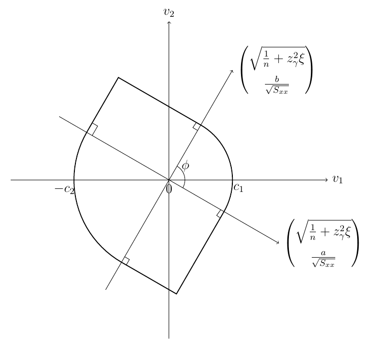
Figure 1: The area of $\bm{R}_{\bm{V}}$

Set $c_{min}=\min(c_{1},c_{2})$ and $c_{max}=\max(c_{1},c_{2})$. The $\text{Area}(\bm{R}_{\bm{V}})$ in (8) can be calculated for the following situations

1. When $\phi<\pi/2$, $\text{Area}(\bm{R}_{\bm{V}})=(c_{min}/\cos\phi+c_{max})^{2}/\tan\phi-c_{min}^{2}\tan\phi+\phi(c_{1}^{2}+c_{2}^{2})/2.$

2. When $\phi=\pi/2$, $\text{Area}(\bm{R}_{\bm{V}})=2c_{1}c_{2}+\phi(c_{1}^{2}+c_{2}^{2})/2.$

3. When $\phi>\pi/2$,

   1. if $c_{min}/\cos(\pi-\phi)>c_{max}$, $\text{Area}(\bm{R}_{\bm{V}})=c_{min}^{2}\tan(\pi-\phi)-(c_{min}/\cos(\pi-\phi)-c_{max})^{2}/\tan(\pi-\phi)+\phi(c_{1}^{2}+c_{2}^{2})/2$;

   2. if $c_{min}/\cos(\pi-\phi)\leq c_{max}$, $\text{Area}(\bm{R}_{\bm{V}})=c_{min}\sqrt{c_{max}^{2}-c_{min}^{2}}+c_{min}^{2}\phi/2+c_{max}^{2}(2\pi-\phi-2\arccos(c_{min}/c_{max}))/2$.

2.2 Confidence Level of Confidence Set

From the construction of SCBs, the critical constants $c_{1}$ and $c_{2}$ are determined from $P\{\bm{V}\in\bm{R_{V}}\}=1-\alpha$. The confidence set $\bm{R_{V}}$ in Figure 1 is partitioned into four triangles $\bm{R}_{\bm{V};M_{i}}$ and four fans $\bm{R}_{\bm{V};N_{i}}$ ($i=1,2,3,4$), see Figure 2. Here, $\phi$ in (10) is partitioned into $\phi_{1}$ and $\phi_{2}$. The angles $\phi_{1}$ and $\phi_{2}$ can be calculated by

$$\cos(\phi_{1}) =\begin{pmatrix}\sqrt{\frac{1}{n}+z_{\gamma}^{2}\xi}\\ 0\end{pmatrix}^{T}\begin{pmatrix}\sqrt{\frac{1}{n}+z_{\gamma}^{2}\xi}\\ \frac{b}{\sqrt{S_{xx}}}\end{pmatrix}\Bigg{/}\left\|\begin{pmatrix}\sqrt{\frac{1}{n}+z_{\gamma}^{2}\xi}\\ 0\end{pmatrix}\right\|\left\|\begin{pmatrix}\sqrt{\frac{1}{n}+z_{\gamma}^{2}\xi}\\ \frac{b}{\sqrt{S_{xx}}}\end{pmatrix}\right\|$$

$$=\frac{\frac{1}{n}+z_{\gamma}^{2}\xi}{\sqrt{[\frac{1}{n}+z_{\gamma}^{2}\xi]\Big{[}\frac{1}{n}+z_{\gamma}^{2}\xi+\frac{b^{2}}{S_{xx}}\Big{]}}},$$

$$\text{and}\ \cos(\phi_{2}) =\begin{pmatrix}\sqrt{\frac{1}{n}+z_{\gamma}^{2}\xi}\\ 0\end{pmatrix}^{T}\begin{pmatrix}\sqrt{\frac{1}{n}+z_{\gamma}^{2}\xi}\\ \frac{a}{\sqrt{S_{xx}}}\end{pmatrix}\Bigg{/}\left\|\begin{pmatrix}\sqrt{\frac{1}{n}+z_{\gamma}^{2}\xi}\\ 0\end{pmatrix}\right\|\left\|\begin{pmatrix}\sqrt{\frac{1}{n}+z_{\gamma}^{2}\xi}\\ \frac{a}{\sqrt{S_{xx}}}\end{pmatrix}\right\|$$

$$=\frac{\frac{1}{n}+z_{\gamma}^{2}\xi}{\sqrt{[\frac{1}{n}+z_{\gamma}^{2}\xi]\Big{[}\frac{1}{n}+z_{\gamma}^{2}\xi+\frac{a^{2}}{S_{xx}}\Big{]}}}.$$

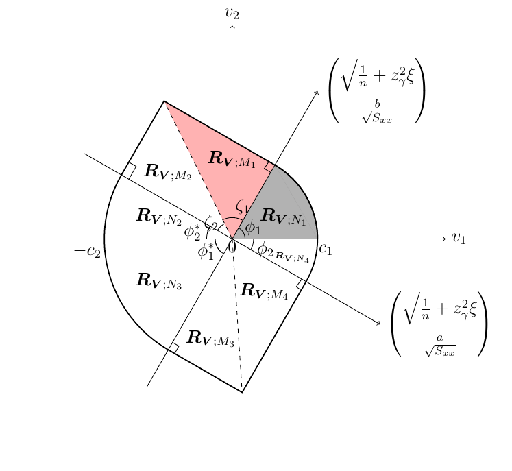
Figure 2: The partitioned regions of $\bm{R_{V}}$

In order to calculate the probability of $\bm{V}$ in $\bm{R_{V}}$, three different situations according to $\phi$ are considered below.

1. When $\phi=\frac{\pi}{2}$, we have $\zeta_{1}=\arctan\left(\frac{c_{max}}{c_{min}}\right)$, $\zeta_{2}=\pi-\zeta_{1}-\phi$, $\phi_{1}^{*}=\phi_{1}$ and $\phi_{2}^{*}=\phi_{2}$.

2. When $\phi<\frac{\pi}{2}$, we have $\zeta_{1}=\arctan\left[\left(\frac{c_{max}}{\cos\phi}+c_{min}\right)\tan\left(\frac{\pi}{2}-\phi\right)/c_{min}\right]$, $\zeta_{2}=\pi-\zeta_{1}-\phi$, $\phi_{1}^{*}=\phi_{1}$ and $\phi_{2}^{*}=\phi_{2}$.

3. When $\phi>\frac{\pi}{2}$,

   1. if $c_{min}/\cos(\pi-\phi)>c_{max}$, we have $\zeta_{1}=\arctan\left[\left(\frac{c_{max}}{\cos(\pi-\phi)}-c_{min}\right)\tan\left(\phi-\frac{\pi}{2}\right)/c_{min}\right]$, $\zeta_{2}=\pi-\zeta_{1}-\phi$, $\phi_{1}^{*}=\phi_{1}$ and $\phi_{2}^{*}=\phi_{2}$;

   2. if $c_{min}/\cos(\pi-\phi)\leq c_{max}$, we have $\zeta_{1}=\arccos\left(\frac{c_{min}}{c_{max}}\right)$, $\zeta_{2}=0$, $\phi_{1}^{*}=\pi-\phi_{2}-\zeta_{1}$, and $\phi_{2}^{*}=\pi-\phi_{1}-\zeta_{1}$.

Define the polar coordinates of $\bm{V}=(V_{1},V_{2})^{T}$, $(R,\delta)$, by

$$V_{1}=R\cos\delta,\ V_{2}=R\sin\delta\ \text{for}\ R>0\ \text{and}\ \delta\in[0,2\pi).$$

The joint density of $(R,\delta)$ is

$$f_{R,\delta}(r,\delta) =f_{V_{1},V_{2}}(v_{1},v_{2})r$$

$$=\frac{r\exp(-q_{3}^{2}/2)\nu^{\nu/2}}{q_{1}2^{\nu/2}\pi\Gamma(\nu/2)}\int_{0}^{\infty}v_{3}^{\nu+1}\exp\Bigg{\{}-\frac{1}{2}\Bigg{[}\left(\left(\frac{r\cos\delta-q_{2}}{q_{1}}\right)^{2}+r^{2}(\sin\delta)^{2}+\nu\right)v_{3}^{2}$$

$$\hskip 213.39566pt+\frac{2q_{3}(r\cos\delta-q_{2})}{q_{1}}v_{3}\Bigg{]}\Bigg{\}}dv_{3}.$$ (11)

where $q_{1}=\sqrt{\frac{1}{1+nz_{\gamma}^{2}\xi}}$, $q_{2}=\frac{z_{\gamma}\sqrt{n}}{\sqrt{\theta^{2}(1+nz_{\gamma}^{2}\xi)}}$ and $q_{3}=z_{\gamma}\sqrt{n}$, the derivation of $f_{V_{1},V_{2}}(v_{1},v_{2})$ in (11) is given in the Appendix.

As pointed out above region $\bm{R_{V}}$ is partitioned in the following way:

$$\bm{R_{V}}=\bm{R}_{\bm{V};M_{1}}+\bm{R}_{\bm{V};M_{2}}+\bm{R}_{\bm{V};M_{3}}+\bm{R}_{\bm{V};M_{4}}+\bm{R}_{\bm{V};N_{1}}+\bm{R}_{\bm{V};N_{2}}+\bm{R}_{\bm{V};N_{3}}+\bm{R}_{\bm{V};N_{4}}$$

where

$$\bm{R}_{\bm{V};M_{1}} =\{\bm{V}:\ \delta\in[\phi_{1},\phi_{1}+\zeta_{1}),\ 0\leq\left(\cos\left(\phi_{1}\right),\sin\left(\phi_{1}\right)\right)\bm{V}\leq c_{1}\}$$

$$=\left\{(R,\delta):\ \delta\in[\phi_{1},\phi_{1}+\zeta_{1}),\ R\leq\frac{c_{1}}{\cos\left(\delta-\phi_{1}\right)}\right\},$$

$$\bm{R}_{\bm{V};M_{2}} =\{\bm{V}:\ \delta\in[\phi_{1}+\zeta_{1},\pi-\phi_{2}^{*}),\ 0\leq\left(\cos\left(\pi-\phi_{2}^{*}\right),\sin\left(\pi-\phi_{2}^{*}\right)\right)\bm{V}\leq c_{2}\}$$

$$=\left\{(R,\delta):\ \delta\in[\phi_{1}+\zeta_{1},\pi-\phi_{2}^{*}),\ R\leq\frac{c_{2}}{\cos\left(\delta-\pi+\phi_{2}^{*}\right)}\right\},$$

$$\bm{R}_{\bm{V};M_{3}} =\{\bm{V}:\ \delta\in[\pi+\phi_{1}^{*},\pi+\phi_{1}^{*}+\zeta_{2}),\ 0\leq\left(\cos\left(\pi+\phi_{1}^{*}\right),\sin\left(\pi+\phi_{1}^{*}\right)\right)\bm{V}\leq c_{2}\}$$

$$=\left\{(R,\delta):\ \delta\in[\pi+\phi_{1}^{*},\pi+\phi_{1}^{*}+\zeta_{2}),\ R\leq\frac{c_{2}}{\cos\left(\delta-\pi-\phi_{1}^{*}\right)}\right\},$$

$$\bm{R}_{\bm{V};M_{4}} =\{\bm{V}:\ \delta\in[\pi+\phi_{1}^{*}+\zeta_{2},2\pi-\phi_{2}),\ 0\leq\left(\cos\left(2\pi-\phi_{2}\right),\sin\left(2\pi-\phi_{2}\right)\right)\bm{V}\leq c_{2}\}$$

$$=\left\{(R,\delta):\ \delta\in[\pi+\phi_{1}^{*}+\zeta_{2},2\pi-\phi_{2}),\ R\leq\frac{c_{2}}{\cos\left(\delta-2\pi+\phi_{2}\right)}\right\},$$

$$\bm{R}_{\bm{V};N_{1}} =\{\bm{V}:\ \delta\in[0,\phi_{1}),\ ||\bm{V}||\leq c_{1}\}=\{(R,\delta):\ \delta\in[0,\phi_{1}),\ R\leq c_{1}\},$$

$$\bm{R}_{\bm{V};N_{2}} =\{\bm{V}:\ \delta\in[\pi-\phi_{2}^{*},\pi),\ ||\bm{V}||\leq c_{2}\}=\{(R,\delta):\ \delta\in[\pi-\phi_{2}^{*},\pi),\ R\leq c_{2}\},$$

$$\bm{R}_{\bm{V};N_{3}} =\{\bm{V}:\ \delta\in[\pi,\pi+\phi_{1}^{*}),\ ||\bm{V}||\leq c_{2}\}=\{(R,\delta):\ \delta\in[\pi,\pi+\phi_{1}^{*}),\ R\leq c_{2}\},$$

$$\bm{R}_{\bm{V};N_{4}} =\{\bm{V}:\ \delta\in[2\pi-\phi_{2},2\pi),\ ||\bm{V}||\leq c_{2}\}=\{(R,\delta):\ \delta\in[\pi,\pi+\phi_{1}^{*}),\ R\leq c_{2}\}.$$

Therefore, we have

$$P\{\bm{V}\in\bm{R}_{\bm{V}}\}= P\{\bm{V}\in\bm{R}_{\bm{V};M_{1}}\}+P\{\bm{V}\in\bm{R}_{\bm{V};M_{2}}\}+P\{\bm{V}\in\bm{R}_{\bm{V};M_{3}}\}+P\{\bm{V}\in\bm{R}_{\bm{V};M_{4}}\}$$

$$+P\{\bm{V}\in\bm{R}_{\bm{V};N_{1}}\}+P\{\bm{V}\in\bm{R}_{\bm{V};N_{2}}\}+P\{\bm{V}\in\bm{R}_{\bm{V};N_{3}}\}+P\{\bm{V}\in\bm{R}_{\bm{V};N_{4}}\}$$

$$= \int_{\phi_{1}}^{\phi_{1}+\zeta_{1}}\int_{0}^{\frac{c_{1}}{\cos\left(\delta-\phi_{1}\right)}}f_{R,\delta}(r,\delta)drd\delta+\int_{\phi_{1}+\zeta_{1}}^{\pi-\phi_{2}^{*}}\int_{0}^{\frac{c_{2}}{\cos\left(\delta+\phi_{2}^{*}-\pi\right)}}f_{R,\delta}(r,\delta)drd\delta$$

$$+\int_{\pi+\phi_{1}^{*}}^{\pi+\phi_{1}^{*}+\zeta_{2}}\int_{0}^{\frac{c_{2}}{\cos\left(\delta-\phi_{1}^{*}-\pi\right)}}f_{R,\delta}(r,\delta)drd\delta+\int_{\pi+\phi_{1}^{*}+\zeta_{2}}^{2\pi-\phi_{2}}\int_{0}^{\frac{c_{1}}{\cos\left(\delta+\phi_{2}-2\pi\right)}}f_{R,\delta}(r,\delta)drd\delta$$

$$+\int_{0}^{\phi_{1}}\int_{0}^{c_{1}}f_{R,\delta}(r,\delta)drd\delta+\int_{\pi-\phi_{2}^{*}}^{\pi}\int_{0}^{c_{2}}f_{R,\delta}(r,\delta)drd\delta+\int_{\pi}^{\pi+\phi_{1}^{*}}\int_{0}^{c_{2}}f_{R,\delta}(r,\delta)drd\delta$$

$$+\int_{2\pi-\phi_{2}}^{2\pi}\int_{0}^{c_{1}}f_{R,\delta}(r,\delta)drd\delta.$$ (12)

Expression (12) gives the confidence level of a two-sided SCB for the percentile line with given $c_{1}$ and $c_{2}$.

From (12), we propose a new method, based on the confidence set of $\bm{V}$, to compute the critical constants $(c_{1},c_{2})$ for SCBs: given sample size $n$, confidence level $1-\alpha$, $\gamma$, and covariate interval of interest $(a,b)$, we can compute the values of $c_{1}$ and $c_{2}$ to satisfy $P\{\bm{V}\in\bm{R}_{\bm{V}}\}=1-\alpha$ and to minimise the area of $\bm{R_{V}}$ simultaneously.

From our numerical investigations, the computation of critical constants only takes 8 seconds for symmetric SCBs and 115 seconds for asymmetric SCBs on an ordinary Window’s PC (Intel(R) Core(TM) i7-6700 CPU with 3.40GHz, 3.41 GHz, RAM 16.0 GB). We additionally use the simulation-based method introduced by Han et al. (2015) to compute the critical constants $(c_{1},c_{2})$. The simulation-based method requires approximately 340 seconds for symmetric SCBs and 500 seconds for asymmetric SCBs, utilising 1,000,000 simulations, on the same Windows PC. Therefore, our newly proposed method is significantly more efficient.

3 Comparisons under the MACS Criterion

In our numerical comparisons, we focus on the case where $a=-b$, i.e., the interval $x-\bar{x}\in(a,b)$ is symmetric about 0. Let $s=b/\sqrt{S_{xx}}$. Note that, the range of $(a,b)$ is large when $s$ is large. In this case, the critical constants $(c_{1},c_{2})$ and so the areas of confidence sets for $\bm{V}$ depend only on $s$, $n$, $\gamma$, and $1-\alpha$. In our numerical comparison, the settings we used are as follows: (i) $\alpha=0.1,0.01$; (ii) $\gamma=0.75,0.95$; (iii) $n=10,100$; and (iv) $s=0.1,1,10$. According to (10), the $\phi$-values for each SCB depend on $a=-b$ and $S_{xx}$ only through $s$. For Type $I$ bands, the $\phi$-values are denoted as $\phi^{I}$ in the Tables below. For Type $II$ bands, the $\phi$-values also depend on different $\xi$-values. Even with different $\xi$-values, the $\phi$-values for all Type $II$ bands remain the same up to two decimal places for given $s$ and $n$, which are denoted by $\phi^{II}$ in the tables below.

Suppose we have two bands $A$ and $B$ with confidence sets $C_{A}(\bm{T}^{*})$ and $C_{B}(\bm{T}^{*})$, respectively. Given the interval of interest $(a,b)$, $n$, $\alpha$, $\gamma$, $\theta$ and $\xi$, the ratio

$$r=\frac{\text{Area}(C_{B}(\bm{T}^{*}))}{\text{Area}(C_{A}(\bm{T}^{*}))}$$

is of interest for comparing bands $A$ and $B$ under MACS criterion. When $r>1$, the area of $C_{A}(\bm{T}^{*})$ is smaller, and so $A$ is better; otherwise, $B$ is better.

Table 2 shows the comparison among Type $I$ bands relative to TBEa band. Table 3 shows the comparison among Type $II$ bands relative to UVa band. According to Table 2, asymmetric Type $I$ bands outperform symmetric Type $I$ bands by up to about 100% when both $1-\alpha$ and $\gamma$ are large. Among the three symmetric Type $I$ bands, TBE has the smallest area of $C(\bm{T}^{*})$, and so TBE is the best in terms of MACS. The difference in the areas of confidence sets among the three asymmetric Type $I$ bands is small. From Table 3, asymmetric Type $II$ bands are better than symmetric Type $II$ bands, by as much as about 78% when $1-\alpha$ is large and $s$ is small. Among the three symmetric Type $II$ bands, V band consistently performs slightly worse than UV band under MACS criterion, and therefore, V band is not recommended. The differences in the areas of confidence sets between UV and TT are small, so either band can be used. Additionally, the differences in the areas of confidence sets among the three asymmetric Type $II$ bands are minor. In general, an asymmetric SCB is better than the corresponding symmetric SCB according to the MACS criterion.

To investigate the performances cross Type $I$ and Type $II$ bands, both symmetric and asymmetric, Table 4 presents the comparison of TBE, TBEa, UV relative to UVa. Notably, UVa performs the best in most cases, while TBEa is the best when the sample size is small and $x$-values in the training dataset are dispersed (i.e. $n=10$ and $s=10$).

Based on the results in Table 4, we conduct a comparison between TBEa and UVa with $n=10$ in Figures 3 and 4. The $\phi^{I}$-values for Type $I$ bands are utilised as $\phi$-axis. Figures 3 and 4 reveal that the $r$ ratio is below 1 for large $\phi$ and $1-\alpha$ (e.g., $\phi>2.8$ and $1-\alpha=0.99$), when the sample size $n$ is small. Therefore, one concludes that TBEa is better than UVa when both $\phi$ and $1-\alpha$ are large, and sample size $n$ is small. It is also noteworthy that $\phi^{I}$ and $\phi^{II}$ are larger than 3 when $s\geq 10$, indicating that $x$-values of training dataset are dispersed. Hence, asymmetric Type $I$ bands should be used only for dispersed $x$-values of training dataset and large confidence level $1-\alpha$, when sample size $n$ is small. Therefore, asymmetric Type $II$ bands, like UVa, are recommanded in general.

Table 2: Ratios $r$, relative to TBEa, of the areas of $C(\bm{T}^{*})$ for symmetric and asymmetric Type $I$ SCBs: SB, TBU, TBE, SBa , TBUa.

$1-\alpha$	$\gamma$	$n$	$s$	$\phi^{I}$	$SB$	$TBU$	$TBE$	$SBa$	$TBUa$
0.9	0.75	10	0.1	0.613	1.038	1.020	1.000	1.000	1.000
			1	2.529	1.039	1.024	1.003	1.003	1.001
			10	3.078	1.038	1.023	1.002	1.008	1.005
		100	0.1	1.571	1.004	1.003	1.002	1.000	1.000
			1	2.942	1.002	1.001	1.000	1.000	1.000
			10	3.122	1.002	1.001	1.000	1.001	1.000
	0.95	10	0.1	0.613	1.158	1.079	1.000	0.999	0.999
			1	2.529	1.158	1.087	1.004	0.977	0.985
			10	3.078	1.160	1.089	1.006	0.965	0.974
		100	0.1	1.571	1.006	1.003	1.000	0.999	1.000
			1	2.942	1.006	1.003	1.000	0.996	0.998
			10	3.122	1.006	1.003	1.000	0.996	0.998
0.99	0.75	10	0.1	0.613	1.322	1.287	1.206	1.000	1.000
			1	2.529	1.243	1.218	1.160	1.006	1.004
			10	3.078	1.226	1.201	1.144	1.014	1.009
		100	0.1	1.571	1.025	1.021	1.014	1.000	1.000
			1	2.942	1.023	1.019	1.013	1.000	1.001
			10	3.122	1.022	1.019	1.013	1.001	1.000
	0.95	10	0.1	0.613	1.807	1.731	1.554	1.000	1.000
			1	2.529	1.921	1.844	1.664	0.974	0.980
			10	3.078	2.004	1.922	1.735	1.006	1.000
		100	0.1	1.571	1.085	1.071	1.046	1.000	1.000
			1	2.942	1.107	1.093	1.067	0.990	0.993
			10	3.122	1.114	1.100	1.074	0.986	0.989

• $\phi^{I}$ is the angle $\phi$ in (10) for symmetric and asymmetric Type $I$ bands ($SB$, $TBU$, $TBE$, $SBa$, $TBUa$ and $TBEa$ bands).

Table 3: Ratios $r$, relative to UVa, of the areas of $C(\bm{T}^{*})$ for symmetric and asymmetric Type $II$ SCBs: V, UV, TT, Va, TTa.

$1-\alpha$	$\gamma$	$n$	$s$	$\phi^{II}$	$V$	$UV$	$TT$	$Va$	$TTa$
0.9	0.75	10	0.1	0.543	1.038	1.020	1.020	1.000	1.000
			1	2.451	1.036	1.022	1.022	1.002	1.000
			10	3.070	1.027	1.014	1.014	1.004	1.000
		100	0.1	1.466	1.002	1.001	1.001	1.000	1.000
			1	2.920	1.002	1.001	1.001	1.000	1.000
			10	3.119	1.001	1.000	1.000	1.001	1.000
	0.95	10	0.1	0.543	1.161	1.081	1.080	1.000	1.000
			1	2.451	1.141	1.092	1.091	1.001	0.999
			10	3.070	1.114	1.070	1.068	1.007	0.998
		100	0.1	1.466	1.007	1.003	1.003	1.000	1.000
			1	2.920	1.006	1.003	1.003	1.001	1.000
			10	3.119	1.005	1.002	1.002	1.001	1.000
0.99	0.75	10	0.1	0.543	1.322	1.286	1.286	1.000	1.000
			1	2.451	1.191	1.168	1.169	1.002	1.000
			10	3.070	1.149	1.128	1.128	1.004	0.999
		100	0.1	1.466	1.024	1.021	1.021	1.000	1.000
			1	2.920	1.016	1.014	1.014	1.001	1.000
			10	3.119	1.015	1.012	1.012	1.000	1.000
	0.95	10	0.1	0.543	1.807	1.731	1.729	1.000	1.000
			1	2.451	1.535	1.476	1.479	1.003	0.999
			10	3.070	1.381	1.328	1.331	1.006	0.998
		100	0.1	1.466	1.085	1.072	1.072	1.000	1.000
			1	2.920	1.059	1.050	1.050	1.001	1.000
			10	3.119	1.055	1.045	1.045	1.001	1.000

• $\phi^{II}$ is the angle $\phi$ in (10) for symmetric and asymmetric Type $II$ bands ($V$, $UV$, $TT$, $Va$, $UVa$ and $TTa$ bands).

Table 4: Ratios $r$, relative to UVa, of the areas of $C(\bm{T}^{*})$ for SCBs: TBE , TBEa, UV.

$1-\alpha$	$\gamma$	$n$	$s$	$\phi^{I}$	$\phi^{II}$	$TBE$	$TBEa$	$UV$
0.9	0.75	10	0.1	0.613	0.543	1.003	1.005	1.022
			1	2.529	2.451	1.008	1.005	1.027
			10	3.078	3.070	0.998	0.994	1.012
		100	0.1	1.571	1.466	1.014	1.012	1.003
			1	2.942	2.920	1.006	1.005	1.002
			10	3.122	3.119	1.004	1.005	1.001
	0.95	10	0.1	0.613	0.543	1.015	1.014	1.082
			1	2.529	2.451	1.120	1.114	1.091
			10	3.078	3.070	1.090	1.085	1.063
		100	0.1	1.571	1.466	1.087	1.088	1.004
			1	2.942	2.920	1.112	1.110	1.003
			10	3.122	3.119	1.111	1.110	1.001
0.99	0.75	10	0.1	0.613	0.543	1.214	1.011	1.291
			1	2.529	2.451	1.152	0.994	1.172
			10	3.078	3.070	1.112	0.973	1.129
		100	0.1	1.571	1.466	1.035	1.019	1.021
			1	2.942	2.920	1.017	1.006	1.010
			10	3.122	3.119	1.016	1.006	1.012
	0.95	10	0.1	0.613	0.543	1.562	1.019	1.720
			1	2.529	2.451	1.766	1.065	1.455
			10	3.078	3.070	1.587	0.915	1.306
		100	0.1	1.571	1.466	1.184	1.138	1.070
			1	2.942	2.920	1.251	1.177	1.046
			10	3.122	3.119	1.239	1.160	1.038

• $\phi^{I}$ is the angle $\phi$ in (10) for Type $I$ bands ($SB$, $TBU$ and $TBE$ bands).

• $\phi^{II}$ is the angle $\phi$ in (10) for Type $II$ bands ($V$, $UV$ and $TT$ bands).

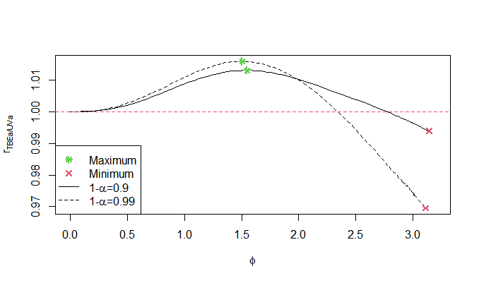
Figure 3: The ratios between TBEa and UVa bands when $\gamma=0.75$, $n=10$ and $\phi\in(0,2\pi)$

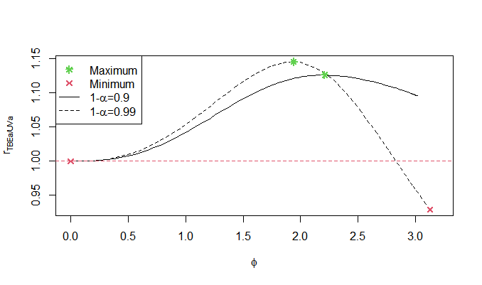
Figure 4: The ratios between TBEa and UVa bands when $\gamma=0.95$, $n=10$ and $\phi\in(0,2\pi)$

4 Real Data Example

In order to illustrate a visual demonstration of SCBs and their corresponding confidence sets $C(\bm{T}^{*})$, a drug stability study based on the observations on the first batch of Experiment One in Ruberg and Hsu (1992) is used as a real data example. Drug stability studies are routinely carried out to understand the degradation over time of a drug product in the pharmaceutical industry. One frequently used statistical model for drug stability studies is the simple linear regression. According to the observations in Ruberg and Hsu (1992), the fitted model is $\hat{y}=98.244-1.515(x-\bar{x})$ with the coefficient of determination $R^{2}=0.9961$, where $\bar{x}=\sum_{i=1}^{n}x_{i}/n=1.482$ and $n=9$.

From patients’ point of view, a large proportion, $1-\gamma$, of all the dosage units should have a drug content level above a pre-specified threshold $h$ before the expiry date. In this case, it is desirable to establish the SCBs for $\bm{x}^{T}\bm{\beta}+z_{\gamma}\sigma$ to study the degradation of this drug product. If the lower confidence band of $\bm{x}^{T}\bm{\beta}+z_{\gamma}\sigma$ is above the threshold $h$ (e.g., for a hypothetic value $h=98$) over time $x\in(a,b)$, it signifies that $1-\gamma$ of all the dosage units have a drug content level above $h$ with confidence $1-\alpha$, and so this drug is still safe to use. Since the expiry date required by the United States Food and Drug Administration (FDA) for drug package labels is generally no longer than two years, it is reasonable to set the time interval as $x\in(0,2)$.

Given the inputs $\bm{Y}$, $\bm{X}$, $(a,b)=(0-\bar{x},2-\bar{x})=(-1.482,0.518)$, $\gamma=0.05$ and $1-\alpha=0.95$, Table 5 shows the ratios of areas of confidence sets among: (i) the symmetric SCBs and (ii) the asymmetric SCBs, over the covariate interval $(a,b)$. It is clear from Table 5 that the areas of confidence set for asymmetric SCBs are substantially smaller than those for symmetric SCBs under MACS criterion. Based on the numerical results, we can conclude that UVa band is the best under MACS criterion in this example.

Table 5: Ratios $r$ of the areas of confidence sets for the example on the drug stability study, relative to UVa band.

Bands	Ratio	Bands	Ratio	Bands	Ratio	Bands	Ratio
SB/UVa	1.579	V/UVa	1.425	SBa/UVa	1.089	Va/UVa	1.002
TBU/UVa	1.472	UV/UVa	1.335	TBUa/UVa	1.089	UVa/UVa	1.000
TBE/UVa	1.235	TT/UVa	1.334	TBEa/UVa	1.091	TTa/UVa	1.000

In order to visually demonstrate the disparity in the areas of confidence sets, $C(\bm{T}^{*})$ for TBE, UV, TBEa and UVa are used in Figure 5. The areas of $C(\bm{T}^{*})$ for TBE, UV, TBEa and UVa are given by solid line, dash line, dash-doted line, and doted line, respectively. It is clear that the area of $C(\bm{T}^{*})$ for UVa is the smallest.

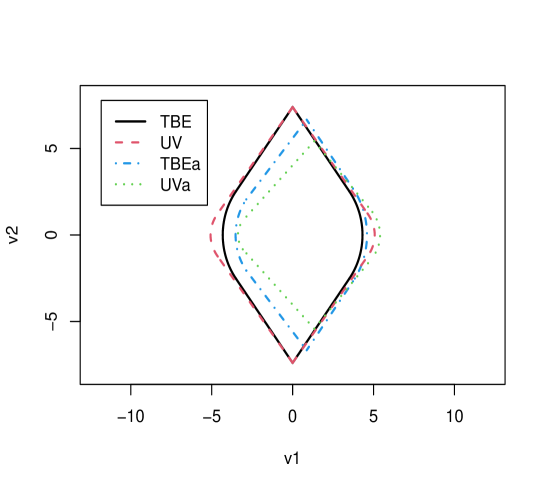
Figure 5: The areas of $C(\bm{T}^{*})$ for bands TBE, UV, TBEa and UVa on coordinate system ($v_{1}$, $v_{2}$)

In Figure 6, the estimated percentile line $\bm{x}^{T}\hat{\bm{\beta}}+z_{\gamma}\hat{\sigma}/\theta$ is shown by the solid line, and the asymmetric Type $II$ band UVa is given by the doted lines. The critical constants ($c_{1}$, $c_{2}$) for UVa are (3.230, 2.016). For the given threshold $h=98$, which is given by the dash-dotted line, one can infer from the band UVa that, the percentile line $\bm{x}^{T}\bm{\beta}+z_{\gamma}\sigma$ is above $h$ before the time point $x=1.326$, and so at least $1-\gamma=95\%$ proportion of all the dosage units have drug content above $h$ by this time point. But beyond the time point $x=1.591$, the percentile line $\bm{x}^{T}\bm{\beta}+z_{\gamma}\sigma$ is below $h$, and so less than 95% proportion of all the dosage units have drug content above $h$. It should be noted that the exact time point $x$ at which $\bm{x}^{T}\bm{\beta}+z_{\gamma}\sigma=h$ can be anywhere in the interval (1.326, 1.591).

In general, according to the area of confidence sets in Figure 5 and the numerical results in Table 5, the asymmetric Type $II$ bands (Va, UVa and TTa) should be used under MACS criterion.

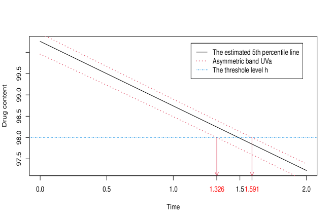
Figure 6: The 95% asymmetric band UVa for the 5th percentile.

5 Conclusion

The MACS criterion is proposed in this paper and it allows the comparison of different types of SCBs for percentiles based on the area of confidence set for the pivotal quantities $\bm{T}^{*}$ related to the unknown parameters $(\bm{\beta},\sigma)$. In addition, our newly proposed MACS-based method of calculating the critical constants for SCBs for percentiles is more computationally efficient than the previous methods available in the statistical literature.

In our paper, it is observed that the areas of confidence set for asymmetric SCBs are uniformly and can be very substantially smaller than those for the corresponding symmetric bands. Asymmetric bands are inherently superior to corresponding symmetric bands according to the MACS criterion, making them the preferred choice. In most cases, asymmetric Type $II$ bands perform better. Therefore, asymmetric Type $II$ bands, like UVa, are recommended.

Although this paper only focuses the simple linear regression model, the proposed method can readily be generalised to multiple linear regression and polynomial regression. Furthermore, the MACS criterion can be used to select optimal simultaneous tolerance intervals for linear regression, which is currently under research and will be reported separately.

Appendix: Joint density function of $(V_{1},V2)$ in $\bm{V}$

Since $N_{1}\sim N(0,1)$, $N_{2}\sim N(0,1)$ and $U\sim\sqrt{\chi_{\nu}^{2}/\nu}$ are independent in (4), the joint density function of $(N_{1},N_{2},U)$ is

$$f(n_{1},n_{2},u)=\frac{\nu^{\nu/2}}{2^{\nu/2}\pi\Gamma(\nu/2)}u^{\nu-1}\exp(-\frac{1}{2}(n_{1}^{2}+n_{2}^{2}+\nu u^{2})).$$ (13)

Now, consider the pdf for $\bm{V}$. We have

$$V_{1}=q_{1}\frac{N_{1}-q_{3}}{U}+q_{2}\ \text{and}\ V_{2}=N_{2}/U,$$

where $q_{1}=\sqrt{\frac{1}{1+nz_{\gamma}^{2}\xi}}$, $q_{2}=\frac{z_{\gamma}\sqrt{n}}{\sqrt{\theta^{2}(1+nz_{\gamma}^{2}\xi)}}$ and $q_{3}=z_{\gamma}\sqrt{n}$. Define the random variable $V_{3}=U$, such that the inverse functions $N_{1}$, $N_{2}$ and $U$ in terms of $V_{1}$, $V_{2}$ and $V_{3}$ are

$$N_{1}=V_{3}\frac{V_{1}-q_{2}}{q_{1}}+q_{3},\ N_{2}=V_{2}V_{3},\ \text{and}\ U=V_{3}.$$ (14)

This implies the following Jacobian matrix and determinant

$$\bm{J} =\begin{pmatrix}\frac{\partial N_{1}}{\partial V_{1}}&\frac{\partial N_{1}}{\partial V_{2}}&\frac{\partial N_{1}}{\partial V_{3}}\\ \frac{\partial N_{2}}{\partial V_{1}}&\frac{\partial N_{3}}{\partial V_{2}}&\frac{\partial N_{3}}{\partial V_{3}}\\ \frac{\partial U}{\partial V_{1}}&\frac{\partial U}{\partial V_{2}}&\frac{\partial U}{\partial V_{3}}\end{pmatrix}=\begin{pmatrix}\frac{V_{3}}{q_{1}}&0&\frac{V_{1}-q_{2}}{q_{1}}\\ 0&V_{3}&V_{2}\\ 0&0&1\end{pmatrix},$$

$$|\bm{J}| =V_{3}^{2}/q_{1}.$$ (15)

With the probability density function of an invertible function, the joint density of $V_{1}$, $V_{2}$ and $V_{3}$ can be derived as

$$f_{V_{1},V_{2},V_{3}}(v_{1},v_{2},v_{3})=f_{\bm{N},U}(n_{1},n_{2},u)|J|.$$

Substituting (14) into (13), and then with (15), we have

$$f_{V_{1},V_{2},V_{3}}(v_{1},v_{2},v_{3})=\frac{\nu^{\nu/2}}{q_{1}2^{\nu/2}\pi\Gamma(\nu/2)}v_{3}^{\nu+1}\exp\Bigg{\{}-\frac{1}{2}\Bigg{[} \left(\left(\frac{v_{1}-q_{2}}{q_{1}}\right)^{2}+v_{2}^{2}+\nu\right)v_{3}^{2}$$

$$+\frac{2q_{3}(v_{1}-q_{2})}{q_{1}}v_{3}+q_{3}^{2}\Bigg{]}\Bigg{\}}.$$

The marginal density of $V_{1}$ and $V_{2}$ can be obtained by integrating out $V_{3}$

$$f_{V_{1},V_{2}}(v_{1},v_{2})=\frac{\exp(-q_{3}^{2}/2)\nu^{\nu/2}}{q_{1}2^{\nu/2}\pi\Gamma(\nu/2)}\int_{0}^{\infty}v_{3}^{\nu+1}\exp\Bigg{\{}-\frac{1}{2}\Bigg{[} \left(\left(\frac{v_{1}-q_{2}}{q_{1}}\right)^{2}+v_{2}^{2}+\nu\right)v_{3}^{2}$$

$$+\frac{2q_{3}(v_{1}-q_{2})}{q_{1}}v_{3}\Bigg{]}\Bigg{\}}dv_{3}.$$

Reference

Al-Saidy, O. M., Piegorsch, W. W., West, R. W., and Nitcheva, D. K. (2003). Confidence bands for low‐dose risk estimation with quantal response data. Biometrics, 59(4), 1056-1062.

Gafarian, A. V. (1964). Confidence bands in straight line regression. Journal of the American Statistical Association, 59(305), 182-213.

Han, Y., Liu, W., Bretz, F., and Wan, F. (2015). Simultaneous confidence bands for a percentile line in linear regression. Computational Statistics and Data Analysis, 81, 1-9.

Liu, W., and Ah-kine, P. (2010). Optimal simultaneous confidence bands in simple linear regression. Journal of statistical planning and inference, 140(5), 1225-1235.

Liu, W., Bretz, F., Hayter, A. J., and Wynn, H. P. (2009). Assessing nonsuperiority, noninferiority, or equivalence when comparing two regression models over a restricted covariate region. Biometrics, 65(4), 1279-1287.

Liu, W., and Hayter, A. J. (2007). Minimum area confidence set optimality for confidence bands in simple linear regression. Journal of the American Statistical Association, 102(477), 181-190.

Liu, W., Jamshidian, M., and Zhang, Y. (2004). Multiple comparison of several linear regression models. Journal of the American Statistical Association, 99(466), 395-403.

Liu, W., Jamshidian, M., Zhang, Y., Bretz, F., and Han, X. L. (2007). Pooling batches in drug stability study by using constant‐width simultaneous confidence bands. Statistics in medicine, 26(14), 2759-2771.

Liu, W., Lin, S., and Piegorsch, W. W. (2008). Construction of exact simultaneous confidence bands for a simple linear regression model. International Statistical Review, 76(1), 39-57.

Piegorsch, W. W., Webster West, R., Pan, W., and Kodell, R. L. (2005). Low dose risk estimation via simultaneous statistical inferences. Journal of the Royal Statistical Society: Series C (Applied Statistics), 54(1), 245-258.

Ruberg, S. J., and Hsu, J. C. (1992). Multiple comparison procedures for pooling batches in stability studies. Technometrics, 34(4), 465-472.

Spurrier, J. D. (1999). Exact confidence bounds for all contrasts of three or more regression lines. Journal of the American Statistical Association, 94(446), 483-488.

Steinhorst, R. K., and Bowden, D. C. (1971). Discrimination and confidence bands on percentiles. Journal of the American Statistical Association, 66(336), 851-854.

Thomas, D. L., and Thomas, D. R. (1986). Confidence bands for percentiles in the linear regression model. Journal of the American Statistical Association, 81(395), 705-708.

Turner, D. L., and Bowden, D. C. (1977). Simultaneous confidence bands for percentile lines in the general linear model. Journal of the American Statistical Association, 72(360a), 886-889.

Turner, D. L., and Bowden, D. C. (1979). Sharp confidence bands for percentile lines and tolerance bands for the simple linear model. Journal of the American Statistical Association, 74(368), 885-888.