Learning the Geodesic Embedding with Graph Neural Networks

Abstract.

We present GeGnn, a learning-based method for computing the approximate geodesic distance between two arbitrary points on discrete polyhedra surfaces with constant time complexity after fast precomputation. Previous relevant methods either focus on computing the geodesic distance between a single source and all destinations, which has linear complexity at least or require a long precomputation time. Our key idea is to train a graph neural network to embed an input mesh into a high-dimensional embedding space and compute the geodesic distance between a pair of points using the corresponding embedding vectors and a lightweight decoding function. To facilitate the learning of the embedding, we propose novel graph convolution and graph pooling modules that incorporate local geodesic information and are verified to be much more effective than previous designs. After training, our method requires only one forward pass of the network per mesh as precomputation. Then, we can compute the geodesic distance between a pair of points using our decoding function, which requires only several matrix multiplications and can be massively parallelized on GPUs. We verify the efficiency and effectiveness of our method on ShapeNet and demonstrate that our method is faster than existing methods by orders of magnitude while achieving comparable or better accuracy. Additionally, our method exhibits robustness on noisy and incomplete meshes and strong generalization ability on out-of-distribution meshes. The code and pretrained model can be found on https://github.com/IntelligentGeometry/GeGnn.

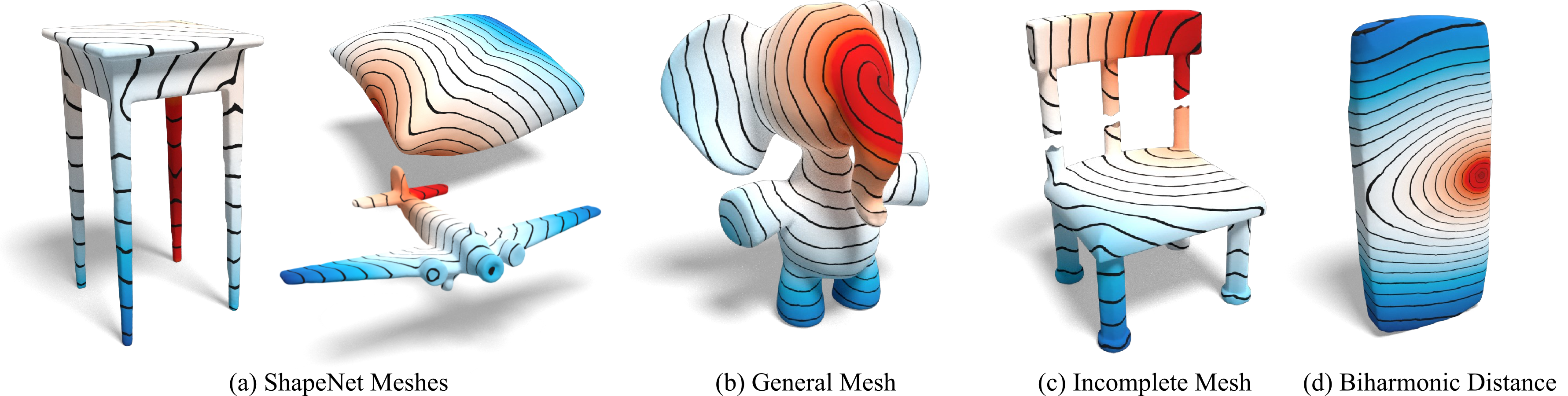
Figure 1. Appealing results produced by our method. The distance fields are color-coded using a gradient ranging from red to blue. (a) We train a graph neural network on ShapeNet to predict the geodesic distances among arbitrary pairs of points on meshes with constant time complexity after a single forward pass as precomputation; the shown results are from the testing set and unseen categories of ShapeNet with an average relative error of less than 1.4% and 2.6%, respectively, which are visually indistinguishable from the ground truth. (b) The network exhibits strong generalization capabilities and can be applied to general meshes out of ShapeNet. (c) The network demonstrates strong robustness on meshes with corrupted topology, which traditional geodesic algorithms cannot handle. (d) Our method is general and can also be used to predict biharmonic distances.

1. Introduction

The computation of the geodesic distance between two arbitrary points on polyhedral surfaces, also referred to as the geodesic distance query (GDQ), is a fundamental problem in computational geometry and graphics and has a broad range of applications, including texture mapping (Zigelman et al., 2002), symmetry detection (Xu et al., 2009), mesh deformation (Bendels and Klein, 2003), and surface correspondence (Raviv et al., 2010). Although plenty of methods (Mitchell et al., 1987; Ying et al., 2013; Adikusuma et al., 2020; Crane et al., 2013b) have been proposed for computing single-source-all-destinations geodesic distances, and some of them can even run empirically in linear time (Crane et al., 2013b; Ying et al., 2013; Tao et al., 2019), it is still too expensive to leverage these methods for GDQs. Consequently, a few dedicated methods (Xin et al., 2012; Panozzo et al., 2013; Xia et al., 2021; Gotsman and Hormann, 2022) have been proposed to ensure that the computation complexity of GDQ is constant to meet the huge requirements of frequent GDQs in interactive applications.

However, these methods either have low accuracy or require long precomputation time, which severely limits their applicability to large-scale meshes. Specifically, in the precomputation stage, these methods typically need to compute the exact geodesic distances between a large number of vertex pairs (Gotsman and Hormann, 2022; Xin et al., 2012; Panozzo et al., 2013; Xia et al., 2021), incurring at least quadratic space and computation complexity; then some methods employ nonlinear optimization (Panozzo et al., 2013; Rustamov et al., 2009) like Metric Multidimensional Scaling (MDS) (Carroll and Arabie, 1998) or cascaded optimization (Xia et al., 2021) to embed the input mesh into a high-dimensional space and approximate the geodesic distance with Euclidean distance in the high-dimensional space, where the optimization process is also time-consuming and costs several minutes, up to hours, even for meshes with tens of thousands of vertices. Additionally, these methods are highly dependent on the quality of input meshes, severely limiting their ability to deal with noisy or incomplete meshes.

In this paper, we propose a learning-based method for const time GDQ on arbitrary meshes. Our key idea is to train a graph neural network (GNN) to embed an input mesh into a high-dimensional feature space and compute the geodesic distance between any pair of vertices with the corresponding feature distance defined by a learnable mapping function. The high-dimensional feature space is referred to as a geodesic embedding of a mesh (Xia et al., 2021; Panozzo et al., 2013). Therefore, our method can be regarded as learning the geodesic embedding with a GNN, instead of relying on costly optimization procedures (Panozzo et al., 2013; Rustamov et al., 2009; Xia et al., 2021); thus, we name our method as GeGnn. After training, our GeGnn can predict the geodesic embedding by just one forward pass of the network on GPUs, which is significantly more efficient than previous optimization-based methods (Xia et al., 2021; Panozzo et al., 2013; Rustamov et al., 2009). Our GeGnn also learns shape priors for geodesic distances during the training process, which makes it robust to the quality of input meshes. As a result, our GeGnn can even be applied to corrupted or incomplete meshes, with which previous methods often fail to produce reasonable results.

The key challenges of our GeGnn are how to design the graph convolution and pooling modules, as well as the mapping function for geodesic distance prediction. Although plenty of graph convolutions have been proposed (Wu et al., 2020) and widely used for learning on meshes (Hanocka et al., 2019; Fey et al., 2018), they are mainly designed for mesh understanding, thus demonstrating inferior performance for our purpose. Our key observation is that the local geometric structures of a mesh are crucial for geodesic embedding. To this end, we propose a novel graph convolution by incorporating local distance features on edges and an adaptive graph pooling module by considering the normal directions of vertices. Our graph convolution follows the message-passing paradigm (Gilmer et al., 2017; Simonovsky and Komodakis, 2017), which updates the vertex feature by aggregating neighboring vertex features. Inspired by the Dijkstra-like methods for computing geodesic distances (Tsitsiklis, 1995; Sethian, 1999) that propagates extremal distance on the wavefront, we propose aggregating local features with the max operator instead of sum or mean, which we find to be much more effective for geodesic embedding.

After embedding an input mesh into a high-dimensional feature space with the proposed GNN, one may naively follow previous works (Panozzo et al., 2013; Rustamov et al., 2009) to use the Euclidean distance in the embedding space between two vertices to approximate the geodesic distance. However, we observe that the Euclidean distance cannot well approximate the geodesic distance, regardless of the dimension of the embedding space. To tackle this issue, we propose to use a lightweight multilayer perceptron (MLP) as a learnable distance function to map the embedding features of a pair of vertices to the geodesic distance, which turns out to work much better than the Euclidean distance.

We train our GeGnn on ShapeNet and verify its effectiveness and efficiency over other state-of-the-art methods for GDQs. Our GeGnn has constant time complexity after a single forward pass of the network as precomputation and linear space complexity, which is much more efficient than previous methods (Xia et al., 2021; Panozzo et al., 2013; Rustamov et al., 2009), with a speedup of orders of magnitude for precomputation and comparable approximation errors for geodesic distances. Our GeGnn also demonstrates superior robustness and strong generalization ability during the inference stage. Finally, we showcase a series of interesting applications supported by our GeGnn.

In summary, our main contributions are as follows:

• We propose GeGnn, a learning-based method for GDQ using a graph neural network with constant time complexity after a single forward pass as precomputation.

• We propose a novel graph convolution module and a graph pooling module, which significantly increase the capability of GeGnn on learning the geodesic embedding.

• We propose to use a learnable distance function to map the embedding features of a pair of vertices to the geodesic distance, resulting in a significant improvement in the approximation accuracy compared with the Euclidean distance.

• We conduct experiments to demonstrate that the proposed framework is robust and generalizable and is also applicable to predict the biharmonic distance.

2. Related Work

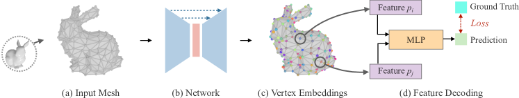
Figure 2. Overview of our GeGnn. We construct a graph from an input mesh (a), and feed the graph to a graph neural network (b). The network architecture follows U-Net. The network lifts every vertex to a high-dimensional embedding space (c). Then we use a lightweight MLP to decode the embeddings of a vertex pair to the corresponding geodesic distance (d). In the training stage, we obtain a loss by comparing the predicted geodesic distance with the precomputed ground truth geodesic distance, which is used to backpropagate through the network and update its parameters. In the testing stage, we can directly use the trained network to predict the vertex features and then compute geodesic distance between any two vertices on the mesh with the MLP.

Single-Source Geodesic Distances

Plenty of algorithms have been developed for the problem of single source geodesic distances computing, we refer the readers to (Crane et al., 2020) for a comprehensive survey. Representative methods include wavefront-propagation-based methods with a priority queue following the classic Dijkstra algorithm (Mitchell et al., 1987; Chen and Han, 1990; Surazhsky et al., 2005; Xin and Wang, 2009; Ying et al., 2014; Xu et al., 2015; Qin et al., 2016), PDE-based methods by solving the Eikonal equation (Sethian, 1999; Kimmel and Sethian, 1998; Mémoli and Sapiro, 2001, 2005; Crane et al., 2013a, 2017), and Geodesic-graph-based methods (Ying et al., 2013; Adikusuma et al., 2020; Sharp and Crane, 2020). There are also parallel algorithms that leverage GPUs for acceleration (Weber et al., 2008). However, the computational cost of these methods is at least linear to the number of vertices, while our method has constant complexity during inference.

Geodesic Distance Queries

The goal of our paper is to approximate the geodesic distance between two arbitrary vertices on a mesh in const time after fast precomputation. The research on this problem is relatively preliminary, and there are only a few related works (Xin et al., 2012; Panozzo et al., 2013; Shamai et al., 2018; Gotsman and Hormann, 2022; Zhang et al., 2023). A naive solution is to compute the geodesic distance between all pairs of vertices in advance and store them in a lookup table. However, this method is not scalable to large meshes due to its quadratic time and space complexity. Xin et al.  (2012) propose to construct the geodesic Delaunay triangulation for a fixed number of sample vertices, compute pairwise geodesic distances, record the distances of each vertex to the three vertices of the corresponding geodesic triangle, and approximate the geodesic distance between two arbitrary vertices using triangle unfolding. Its time and space complexity is quadratic to the number of samples, which is still not scalable to large meshes. Panozzo et al.  (2013) propose to embed a mesh into a high-dimensional space to approximate the geodesic distance between a pair of points with the Euclidean distance in the embedding space, which is realized by optimizing with Metric MDS (Carroll and Arabie, 1998; Rustamov et al., 2009). However, the metric MDS in (Panozzo et al., 2013) involves a complex nonlinear optimization and thus is computationally expensive. Shamai et al.  (2018) solve pairwise geodesics employing a fast classic MDS, which extrapolates distance information obtained from a subset of points to the remaining points. Xia et al.  (2021) propose to compute the geodesic embedding by cascaded optimization on a proximity graph containing a subset of vertices (Ying et al., 2013). Likewise, the computational expense of this optimization process makes it impractical for large meshes. Recently, Gotsman et al.  (2022) propose to compress the pairwise geodesic distances by a heuristic divide and conquer algorithm, but its worst case time complexity for GDQ is not constant. In contrast, our GeGnn needs no expensive precomputation and has remarkable efficiency for GDQ, thus is scalable to large meshes. Concurrently, Zhang et al.  (2023) also propose to use neural networks for GDQs; however, this method concentrates on learning on a single mesh, while our method is trained on a large dataset to achieve the generalization capability across different meshes.

Other Geometric Distances

Apart from the geodesic distance, there are also several other distances on meshes. The diffusion distance (Coifman et al., 2005) is defined by a diffusion process on the mesh and is widely used for global shape analysis. The commute-time distance (Fouss et al., 2007; Yen et al., 2007) is intuitively described by the expected time for a random walk to travel between two vertices. The biharmonic distance (Lipman et al., 2010) can be calculated by the solution of the biharmonic equation. The earth mover’s distance (Solomon et al., 2014) is defined by the minimum cost of moving the mass of one point cloud to another. Apart from geodesic distances, our GeGnn can also be easily extended to approximate these distances by replacing the geodesic distance with the corresponding distance in the loss function. We showcase the results of approximating the biharmonic distance in our experiments.

Graph Neural Networks

Graph neural networks (GNN) have been widely used in many applications (Wu et al., 2020). As the core of a GNN, a graph convolution module can be formulated under the message passing paradigm (Gilmer et al., 2017; Simonovsky and Komodakis, 2017). Representative GNNs include the graph convolutional network (Kipf and Welling, 2017), the graph attention network (Velickovic et al., 2017), and GraphSAGE (Hamilton et al., 2017). Many point-based neural networks for point cloud understanding (Qi et al., 2017; Li et al., 2018; Thomas et al., 2019; Xu et al., 2018a; Wang et al., 2019) can be regarded as special cases of graph neural networks on k-nearest-neighbor graphs constructed from unstructured point clouds. Graph neural networks can also be applied to triangle meshes for mesh understanding (Hanocka et al., 2019; Hu et al., 2022; Yi et al., 2017), simulation (Pfaff et al., 2020), processing (Liu et al., 2020), and generation (Hanocka et al., 2020). However, these methods are not specifically designed for GDQs and demonstrate inferior performance compared to our dedicated graph convolution in terms of approximation accuracy.

3. Method

Overview

The overall pipeline of our GeGnn is shown in Fig. 2. Our method can be roughly separated into two parts: precomputation, and geodesic distance query (GDQ) . The precompuation step (Fig. 2 (b)) involves evaluating a graph neural network to obtain vertex-wise features of fixed dimension. This step is performed only once for each mesh, regardless of the number of subsequent queries. The geodesic distance query (Fig. 2 (d)) involves forwarding the powered difference between two features to a fixed size MLP. This process requires a fixed number of max/add/multiplication operations for each query, resulting in a time complexity of $O(1)$ for GDQ. Specifically, given an input mesh $\mathcal{M}=\{\mathcal{V},\mathcal{F}\}$, where $\mathcal{V}$ and $\mathcal{F}$ denote the set of vertices and faces of the mesh, the connectivity of the mesh defined by $\mathcal{F}$ naturally forms a graph $\mathcal{G}$. We first train a graph neural network that takes $\mathcal{G}$ and $\mathcal{V}$ as input and maps each vertex $v_{i}$ in $\mathcal{V}$ to a high dimensional embedding vector $p_{i}\in\mathbb{R}^{c}$, where $c$ is set to 256 by default. We construct a U-Net (Ronneberger et al., 2015) on the graph to effectively extract features for each vertex. Then we use a lightweight MLP to take the features of two arbitrary vertices as input and output the corresponding geodesic distance between them. The key building blocks of our network include a novel graph convolution module and a graph pooling module, which are elaborated in Section 3.1. The feature decoding scheme for geodesic distance prediction is elaborated in Section 3.2. Finally, the network details and the loss function are introduced in Section 3.3.

3.1. Graph Neural Network

In this section, we introduce our graph convolution and pooling modules tailored for learning the geodesic embedding, which serve as the key building blocks of our network.

3.1.1. Graph Convolution

The graph convolution module is used to aggregate and update features on a graph. The graph $\mathcal{G}$ constructed from an input mesh $\mathcal{M}=\{\mathcal{V},\mathcal{F}\}$ contains the neighborhood relationships among vertices. For the $i^{th}$ vertex $v_{i}$ in $\mathcal{V}$, we denote the set of its neighboring vertices as $\mathcal{N}(i)$ and its feature as $F_{i}$. Generally, denote the output of the graph convolution module as $F_{i}^{\prime}$, the module under the message passing paradigm (Gilmer et al., 2017; Simonovsky and Komodakis, 2017; Fey and Lenssen, 2019) can be defined as follows:

(1) $$F_{i}^{\prime}=\gamma\left(F_{i},\;\mathcal{A}_{j\in\mathcal{N}(i)}\phi\left(F_{i},F_{j},v_{i},v_{j}\right)\right),$$

where $\gamma$ and $\phi$ are differentiable functions for updating features, and $\mathcal{A}$ is a differentiable and permutation invariant function for aggregating neighboring features, e.g., sum, mean, or max. The key difference among different graph convolution operators lies in the design of $\gamma$, $\phi$, and $\mathcal{A}$.

Although plenty of graph convolutions have been proposed, they are mainly used for graph or mesh understanding (Fey et al., 2018; Velickovic et al., 2017; Kipf and Welling, 2017) and are insensitive to the local distances between vertices, which are crucial for geodesic embedding. Our design philosophy is to explicitly incorporate the distances between neighboring vertices into the graph convolution, with a focus on maximizing simplicity while maintaining expressiveness. Therefore, we define the functions for updating features $\phi$ and $\gamma$ as follows:

(2) $$\gamma(F_{i},\bar{F}_{i}) =W_{0}\times F_{i}+\bar{F}_{i},$$

(3) $$\phi\left(F_{i},F_{j},v_{i},v_{j}\right) =W_{1}\times[F_{j}\mathbin{\|}v_{ij}\mathbin{\|}l_{ij}],$$

where $\bar{F}_{i}=\mathcal{A}_{j\in\mathcal{N}(i)}\phi\left(F_{i},F_{j},v_{i},v_{j}\right)$, $W_{0}$ and $W_{1}$ are trainable weights, $\mathbin{\|}$ is a concatenation operator, $v_{ij}$ is a shorthand for $v_{i}-v_{j}$, and $l_{ij}$ is the length of $v_{ij}$. For the aggregation operator, we choose max, instead of sum or mean, which is motivated by Dijkstra-like methods for computing geodesic distances (Tsitsiklis, 1995; Sethian, 1999) that propagate the shortest distance on the wavefront. This choice is also consistent with the observation in (Xu et al., 2018b) that the max is advantageous in identifying representative elements. In summary, our graph convolution is defined as follows:

(4) $$F_{i}^{\prime}=W_{0}\times F_{i}+\max\nolimits_{j\in\mathcal{N}(i)}\left(W_{1}\times[F_{j}\mathbin{\|}v_{ij}\mathbin{\|}l_{ij}]\right),$$

Since our graph convolution is designed for geodesic embedding, we name it as GeoConv. According to Eq. 4, our GeoConv does not use any global information such as absolute positions, and thus is translation and permutation invariant by design, which are desired properties for geodesic computing.

Compared with previous graph convolutions in the field of 3D deep learning (Wang et al., 2019; Simonovsky and Komodakis, 2017) that define $\phi$ or $\gamma$ as MLPs, our GeoConv is much simpler, while being more effective for geodesic embedding, as verified in our experiments and ablation studies. Our GeoConv is reminiscent of GraphSAGE (Hamilton et al., 2017) for graph node classification on citation and Reddit post data; however, GraphSAGE does not consider local distances between vertices and uses mean for aggregation, resulting in an inferior performance for geodesic embedding.

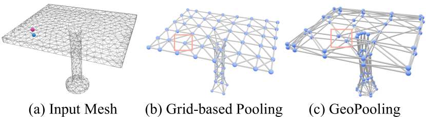
Figure 3. Comparison of graph pooling strategies. (a) The red and blue vertices are located on opposite sides of the tabletop. Although they are distant in terms of geodesic distance, they are close in Euclidean space. (b) The grid-based pooling merges the red and blue vertices into a single vertex, which is inadequate for geodesic embedding. (c) Our GeoPool is capable of preserving the geodesic distance and effectively distinguishing between the red and blue vertices.

3.1.2. Graph Pooling

Graph pooling is used to progressively downsample the graph to facilitate the construction of U-Net. Representative graph pooling designs in previous works are either based on mesh simplification with a priority queue (Hanocka et al., 2019) or leverage farthest point sampling (Qi et al., 2017), incurring huge computational cost and diffculties concerning parallelism. Therefore, we resort to grid-based graph pooling for efficiency (Hu et al., 2020; Thomas et al., 2019; Simonovsky and Komodakis, 2017). Grid-based pooling employs regular voxel grids to cluster vertices within the same voxel into a single vertex, resulting in a straightforward and efficient way to downsample the graph. Nevertheless, grid-based pooling only relies on the Euclidean distance of vertices and ignores the topology of the underlying graph or mesh. An example is shown in Fig. 3-(a): the red and blue vertices are on the opposite sides of the tabletop; they are far away in terms of geodesic distance but close in Euclidean space. Grid-based pooling may merge these two vertices into a single vertex as shown in Fig. 3-(b), which is undesirable for geodesic embedding.

To address this issue, we propose a novel graph pooling, called GeoPool, which is aware of both Euclidean and geodesic distances. Specifically, we construct regular grids in 6D space consisting of vertex coordinates and the corresponding normals. We specify two scale factors, $\sigma_{c}$ for the coordinates and $\sigma_{n}$ for the normals, to control the size of the grids in different dimensions. Then we merge vertices within the same grid in 6D space and compute the averages of coordinates, normals, and associated features as the output. The use of normals can effectively prevent vertices on the opposite sides of a thin plane from being merged when downsampling the graph. As shown in Fig. 3-(c), the red and blue vertices are in different grids in 6D space, and thus are not merged into a single vertex with GeoPool. Note that GeoPool reduces to vanilla grid-based pooling when $\sigma_{n}$ is set to infinity.

We also construct a graph unpooling module, named GeoUnpool, for upsampling the graph in the decoder of U-Net. Specifically, we keep track of the mapping relation between vertices before and after the pooling operation, and GeoUnpool is performed by reversing the GeoPool with the cached mapping relation.

3.1.3. Network Architecture

We construct a U-Net (Ronneberger et al., 2015) with our GeoConv, GeoPool, and GeoUnpool modules, as shown in Fig. 4. The network takes the graph constructed from an input mesh as input. The initial vertex signals have 6 channels, including the normalized vertex coordinates and normals. The vertex features are updated by GeoConv; and each GeoConv is followed by a ReLU activation and a group normalization (Wu and He, 2018). The ResBlock in Fig. 4 is built by stacking 2 GeoConv modules with a skip connection (He et al., 2016). The output channels of each GeoConv are all set to 256. The graph is progressively downsampled and upsampled by GeoPool and GeoUnpool. Since the input mesh is first normalized into $[-1,1]$, $\sigma_{c}$ and $\sigma_{n}$ are initially set to $1/16$ and $3/16$, and increase by a factor of 2 after each pooling operation. Overall, the U-Net extracts a feature for every vertex, which is then mapped to 256 channels as the geodesic embedding using a MLP consisting of two fully-connected layers with 256 channels.

The geodesic distance between two arbitrary vertices is determined by the shortest path between them, which is a global property of the mesh. The U-Net built upon our graph modules has global receptive fields, while being aware of local geometric structures, which is advantageous for geodesic embedding. The multi-resolution structure of U-Net also increases the robustness when dealing with incomplete meshes, since the missing edges or isolated vertices in incomplete meshes can be merged and get connected in coarser resolutions. We verify the robustness of our network in the experiments.

3.2. Geodesic Decoder

The graph network outputs a geodesic embedding $p_{i}\in\mathbb{R}^{256}$ for each vertex $v_{i}$. To approximate the geodesic distance between vertex $v_{i}$ and $v_{j}$, we need to define a distance function $d(p_{i},p_{j})$ in the embedding space as the decoder. An intuitive strategy is to directly use the Euclidean distance between $p_{i}$ and $p_{j}$, following (Panozzo et al., 2013; Rustamov et al., 2009): $d(p_{i},p_{j})=||p_{i}-p_{j}||_{2}$. However, such an Euclidean embedding is unattainable in most scenarios, including curved surfaces with non-zero Gaussian curvature (Pressley and Pressley, 2010) and finite metric spaces with Gramian matrices that lack positive semidefiniteness (Maehara, 2013).

Here is a simple example to illustrate the issue. Denote the geodesic distance between point $X$ and point $Y$ as $d_{XY}$. For a unit circle depicted on the right, we can easily compute that $d_{AC}=d_{BC}=\pi/2$ and $d_{AB}=\pi$. If we embed this circle into a high-dimensional Euclidean space $\mathcal{X}$, we will have $C$ at the midpoint of the segment $AB$ in $\mathcal{X}$. Similarly, when considering $A$, $B$, and $D$, we know that $D$ is also the midpoint of the segment $AB$. Therefore, $C$ and $D$ would be at the same point in $\mathcal{X}$; however, $d_{CD}$ is equal to $\pi$ on the circle. This example shows that the Euclidean distance cannot well approximate the geodesic distance even on a circle, which is irrelevant to the dimension of the embedding space.

Previous efforts have also attempted manual design of embedding spaces (Shamai et al., 2018), which involves mapping data onto a sphere. Instead of manually designing the decoding function $d(p_{i},p_{j})$, which turns out to be tedious and hard according to our initial experiments, we propose to learn it from data. Specifically, we train a small MLP with 3 fully connected layers and ReLU activation functions in between to learn the decoding function, as shown in Fig. 2-(d). The channels of the decoding MLP are set to 256, 256, and 1, respectively. Define $p_{i}=\left(p_{i,1},\;p_{i,2},\;\dots,\;p_{i,n}\right)$, where $p_{i,k}$ is the $k^{th}$ components of $p_{i}$ and $n$ is the dimension of $p_{i}$, the MLP takes the squared difference $s_{ij}$ between $p_{i}$ and $p_{j}$ as the input:

(5) $$s_{ij}=\left(\left(p_{i,1}-p_{j,1}\right)^{2},\;\left(p_{i,2}-p_{j,2}\right)^{2},\;\dots,\;\left(p_{i,n}-p_{j,n}\right)^{2}\right),$$

and the output of the MLP approximates the geodesic distance between $v_{i}$ and $v_{j}$: $d(p_{i},p_{j})=MLP(s_{ij})$. The square operation in Eq. 5 is necessary as it preserves the symmetry of $d(p_{i},p_{j})$ with respect to $p_{i}$ and $p_{j}$.

Since the MLP only contains 3 layers, its execution on GPUs is very efficient. For each input mesh, we forward the U-Net once to obtain the geodesic embedding of each vertex and cache the results; then each batch of GDQs only requirs a single evaluation of the MLP.

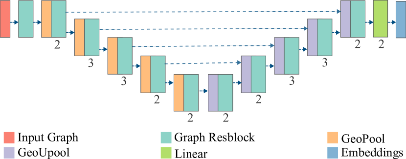
Figure 4. U-Net constructed with our basic network modules. The network takes a graph as input and outputs high-dimensional geodesic embeddings for vertices. The feature channels are all set to 256, and the numbers of each block are shown underneath.

3.3. Loss Function

We adopt the mean relative error (MRE) as the loss function for training, which is also used as the evaluation metric to assess the precision of predicted geodesic distances following (Surazhsky et al., 2005; Xia et al., 2021).

In the data preparation stage, we precompute and store $N$ pairs of exact geodesic distances for each mesh with the method proposed in (Mitchell et al., 1987). In each training iteration, we randomly sample a batch of meshes from the training set, then randomly sample $n$ pair of vertices from the precomputed geodesic distances for each mesh. The MRE for each mesh can be defined as follows:

(6) $$L=\frac{1}{n}\sum\nolimits_{(i,j)\in\mathcal{I}}\frac{|d(p_{i},p_{j})-d_{ij}|}{d_{ij}+\epsilon},$$

where $\mathcal{I}$ is the set of sampled vertex pairs, $d_{ij}$ is the ground-truth geodesic distance between vertex $v_{i}$ and vertex $v_{j}$, $d(p_{i},p_{j})$ is the decoding function described in Section 3.2, and $\epsilon$ is a small constant to avoid numerical issues. In our experiments, we set $N$ to $600k$, $n$ to $100k$, and $\epsilon$ to $0.001$.

Remark

Although our main goal is to predict the geodesic distance, our method is general and can be trivially applied to learn other forms of distances. For example, we precompute Biharmonic distances (Lipman et al., 2010) for certain meshes and use them to replace the geodesic distances in Eq. 6 to train the network. After training, our network can learn to estimate the Biharmonic distances as well. We verify this in our experiments, and we expect that our method has the potential to learn other types of distances as well, which we leave for future work.

4. Results

In this section, we validate the efficiency, accuracy, and robustness of our GeGnn on the task of GDQ and demonstrate its potential applications. We also analyze and discuss key design choices of GeGnn in the ablation study. The experiments were conducted using 4 Nvidia 3090 GPUs with 24GB of memory.

4.1. Geodesic Distance Queries

Dataset

We use a subset of ShapeNet (Chang et al., 2015) to train our network. The subset contains 24,807 meshes from 13 categories of ShapeNet, of which roughly 80% are used for training and others for testing. Since the meshes from ShapeNet are non-manifold, prohibiting the computation of ground-truth geodesic distances, we first convert them into watertight manifolds following (Wang et al., 2022). Then, we apply isotropic explicit remeshing (Bhat et al., 2004; Hoppe et al., 1993) to make the connectivity of meshes regular. Next, we do mesh simplification (Garland and Heckbert, 1997) to collapse 15% of the edges, which diversifies the range of edge length and potentially increases the robustness of our network. The resulting meshes have an average of 5,057 vertices. We normalize the meshes in $[-1,1]$ and leverage the MMP method (Mitchell et al., 1987) to calculate the exact geodesic distance of $600k$ pairs of points on each mesh, which takes 10-15s on a single CPU core for each mesh.

Settings

We employ the AdamW optimizer (Loshchilov and Hutter, 2019) for training, with an initial learning rate of 0.0025, a weight decay of 0.01, and a batch size of 40. We train the network for 500 epochs and decay the learning rate using a polynomial function with a power of 0.9. We implemented our method with PyTorch (Paszke et al., 2019); the training process took 64 hours on 4 Nvidia 3090 GPUs. We use the mean relative error (MRE) defined in Eq. 6 to compare the accuracy of the predicted geodesic distance. To compute the MRE, we randomly sample $500$ vertices, calculate the geodesic distances from each vertex and all other vertices within a given mesh, and then compute the average error between the predicted distances and the ground-truth distances. We use the average time required of 1 million geodesic queries and pre-processing time to evaluate the efficiency. We choose three groups of meshes for evaluation:

• ShapeNet-A: 100 meshes from the testing set of ShapeNet, whose categories are included in the training set. The average number of vertices is 5,057.

• ShapeNet-B: 50 meshes from the ShapeNet, whose categories are different from the 13 categories of the training set. The average number of vertices is 5,120.

• Common: 10 meshes that are not contained in ShapeNet, such as Elephant, Fandisk, and Bunny. The topologies, scales, and geometric features of these meshes are significantly different from those in ShapeNet. The average number of vertices is 7,202.

Several examples from these three groups of meshes are shown in Fig. 5. The meshes from ShapeNet-B and Common are used to test the generalization ability of our method when dealing with out-of-distribution meshes.

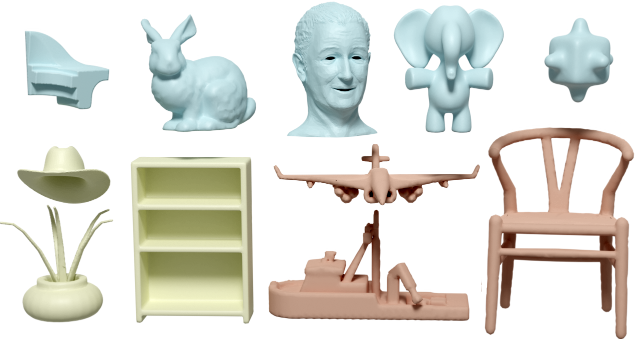
Figure 5. Example meshes for evaluation. The meshes from the ShapeNet-A, ShapeNet-B, and Common groups are shown in red, yellow, and blue, respectively. Notice that our network can handle meshes with boundaries: the head (MRE=2.0%) has open boundaries near its eyes and neck.

Comparisons

We compare our method with several state-of-the-art methods on geodesic distance queries (GDQs). MMP (Mitchell et al., 1987) is a classic method for computing geodesic distances, with a time complexity of $\mathcal{O}(N^{2}\log N)$ for each GDQ, where $N$ is the number of mesh vertices. MMP does not require precomputation and produces exact geodesic distances, which are used for reference. The Heat Method (HM) (Crane et al., 2013b, 2017) computes geodesic distances by solving a heat equation and a Poisson equation on meshes, with a time complexity of $\mathcal{O}(N)$ for each GDQ after matrix factorization of the involved linear system. The Discrete Geodesic Graphs (DGG) (Adikusuma et al., 2020) construct an undirected and sparse graph for computing discrete geodesic distances on triangle meshes and requires $\mathcal{O}(N)$ time for each GDQ. The optimization-based methods, including the Euclidean Embedding Method (EEM) (Panozzo et al., 2013) and the Geodesic Embedding (GE) (Xia et al., 2021), leverage costly cascaded non-linear optimization to compute the geodesic embedding of a mesh, with a time complexity of $\mathcal{O}(1)$ for each GDQ. The precomputation time of FPGDC (Shamai et al., 2018) depends on its sample number $k$, with a time complexity of $\mathcal{O}(1)$ for each GDQ. Our method produces the geodesic embedding by a forward evaluation of a GNN and has a time complexity of $\mathcal{O}(1)$ for each GDQ. We compare our method with the above methods on the three groups of meshes using the code provided by the authors or publicly available on the web. Previous methods are mainly developed with C++ and run on CPU, and it is non-trivial for us to reimplement them on GPU; we thus run them on top of a Windows computer with a Ryzen R9 5900HX CPU and 32GB of memory. We keep their default parameter settings unchanged during the evaluations unless specified. We evaluate our method on a single RTX 3090 GPU with a batch size of 10.

Table 1. Performances comparisons on geodesic distance queries. Algorithms specifically designed for GDQ are in bold. PC represents the average time of precomputation for GQDs. GDQ represents the average time of 1 million GDQs after any precomputation. MRE represents the mean relative error. Compared with the state-of-the-art methods, including MMP (Mitchell et al., 1987), HM (Crane et al., 2013b, 2017), DGG (Adikusuma et al., 2020), EEM (Panozzo et al., 2013), FPGDC (Shamai et al., 2018) and GE (Xia et al., 2021), our GeGnn achieves comparable accuracies while being significantly faster in terms of both precomputation and GDQs by orders of magnitude, as indicated in the Speedup column with green color.

Method	Complexity	Speedup	Metric	ShapeNet-A	ShapeNet-B	Common
				5,057	5,120	7,202
MMP	$\mathcal{O}(N^{2}\log N)$	$1.7\!\times\!10^{6}$	GDQ	15.85h	18.00h	25.41h
HM	$\mathcal{O}(N)$	$6.7\!\times\!10^{4}$	GDQ	2345s	2406s	3506s
			MRE	2.41%	2.04%	1.46%
DGG	$\mathcal{O}(N)$	$3.2\!\times\!10^{4}$	GDQ	1163s	1157s	1626s
			MRE	0.27%	0.27%	0.50%
		$4.1\!\times\!10^{2}$	PC	45.02s	30.87s	41.21s
EEM	$\mathcal{O}(1)$	$3.2\!\times\!10^{0}$	GDQ	0.134s	0.120s	0.136s
			MRE	8.11%	8.78%	5.64%
		$7.1\!\times\!10^{1}$	PC	5.64s	6.28s	8.23s
FPGDC	$\mathcal{O}(1)$	$6.2\!\times\!10^{1}$	GDQ	2.75s	2.37s	2.56s
			MRE	2.50%	2.30%	2.30%
GE	$\mathcal{O}(1)$	$3.2\!\times\!10^{3}$	PC	225.5s	297.8s	387.8s
			PC	0.089s	0.091s	0.104s
GeGnn	$\mathcal{O}(1)$		GDQ	0.042s	0.040s	0.041s
			MRE	1.33%	2.55%	2.30%

Speed

The key benefit of our method is its efficiency in terms of both precomputation and GDQs compared with the state-of-the-art methods. The results are summarized in Table 1. Since MMP, HM, and DGG are targeted at computing single-source-all-destinations geodesic distances, our method is at least $\mathbf{3.2\times 10^{4}}$ times faster than them when computing GDQs. Compared with EEM, GE and FPGDC, which all have $\mathcal{O}(1)$ complexity for GDQs, in terms of precomputation, our method is $\mathbf{3.2\times 10^{3}}$ times faster than GE, $\mathbf{4.1\times 10^{2}}$ times faster than EEM, $\mathbf{71}$ times faster than FPGDC with its parameter $N$ set to 400. Here, the precomputation time is the time required to compute the geodesic embedding of a mesh, which is not applicable to MMP, HM, and SVG. The precomputation of our GeGnn involves a single forward pass of the network, which is trivially parallelized on GPUs. In contrast, the precomputation of GE, FPGDC and EMM requires a costly non-linear optimization process or eigen decomposition, which is hard to take advantage of GPU parallelism without sophisticated optimization efforts. Additionally, each GDQ of our method only involves a few matrix products, which are also highly optimized and parallelized on GPUs, whereas the GDQ of GE involves geodesic computation with the help of saddle vertex graphs. We did not calculate the GDQ and MRE of GE in Table 1 since the authors only provided the code for precomputation.

Accuracy

In Table 1, MMP (Mitchell et al., 1987) computes the exact geodesic distances, which is used as the ground truth; the other methods compute approximate geodesic distances. We observe that the accuracy of FPGDC is severely affected by the sample number. With sample number 20 (the default value), its MRE is 12%, much worse than the other methods. Therefore, we set its sample number $k$ to $400$, with which it achieves an accuracy that is slightly worse than ours. Note that FPGDC fails on over 5% of samples in ShapeNet-A and ShapeNet-B; EEM also fails on around 2% meshes. We exclude those failed samples when computing their accuracies. It can be seen that the accuracy of our GeGnn is significantly better than EEM (Panozzo et al., 2013), and our GeGnn even outperforms the Heat Method (Crane et al., 2013b, 2017) on ShapeNet-A. However, our accuracy is slightly worse than DGG (Adikusuma et al., 2020). Nevertheless, we emphasize that it does not affect the applicability of our method in many graphics applications with a mean relative error of less than 3%, including texture mapping, shape analysis as verified in Section 4.3, and many other applications as demonstrated in EEM (Panozzo et al., 2013), of which the mean relative error is above 8% on ShapeNet.

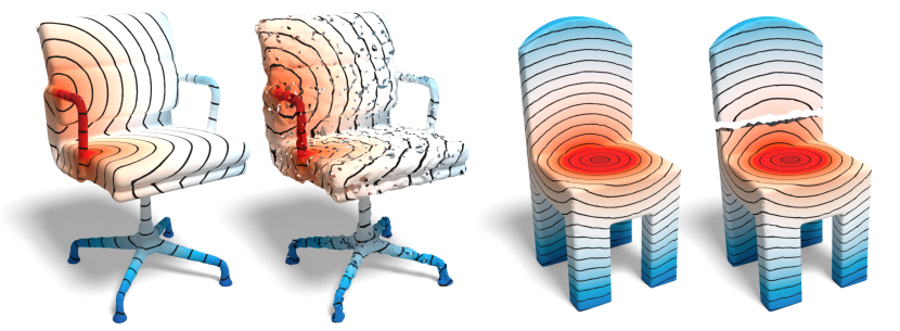
Figure 6. Robustness of our method. Left: the result on an incomplete and noisy mesh. Right: the result on a mesh containing two separated parts.

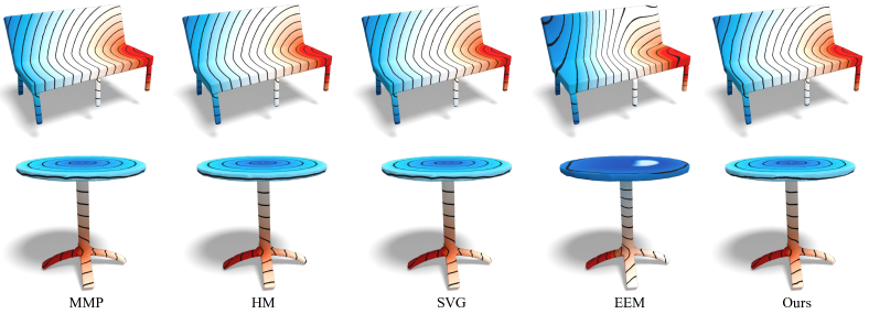
Figure 7. Visual Comparisons. We compared our results with the results of MMP (Mitchell et al., 1987), DDG (Adikusuma et al., 2020), EEM (Panozzo et al., 2013), and HM (Crane et al., 2017). All methods apart from EEM get visually pleasing results.

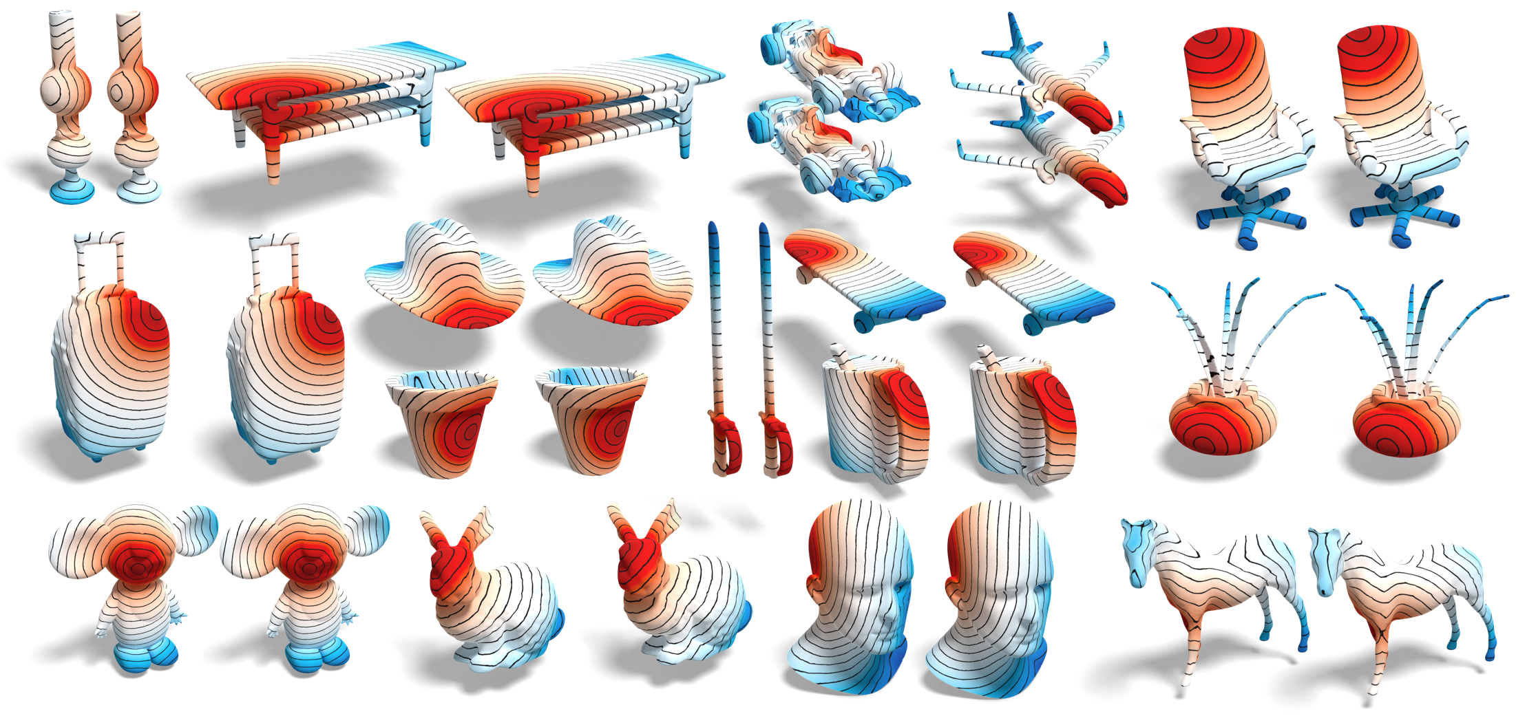
Figure 8. More results on meshes with complex geometric or topological structures. For each pair of meshes, our results are shown on the left or top side, and the corresponding ground truth results are shown on the right or bottom side. The meshes from top to bottom are selected from ShapeNet-A, ShapeNet-B, and Common, respectively. These results demonstrate the effectiveness and strong generalization ability of our method.

Visual Results

We compare the geodesic distances of our method with other methods in Fig. 7. And we show more geodesic distance fields generated by our method in Fig. 8 on various shapes from group ShapeNet-A, ShapeNet-B, and Common in each of the three rows, respectively. These results demonstrate the effectiveness of our GeGnn in computing geodesic distances on meshes with different topologies and geometries, such as those with high genus, curved surfaces, and complex features. It is worth highlighting that our network is trained on ShapeNet-A, and it can generalize well to ShapeNet-B and Common, which demonstrates the strong generalization ability of our method.

Robustness

After training, our GeGnn learns shape priors from the dataset, endowing it with strong robustness to incomplete or noisy meshes. On the left of Fig. 6, we randomly remove 15% of the triangles and add a Gaussian noise with a standard deviation of 0.06 on every vertex. Applying our method to the incomplete and noisy mesh results in an MRE of 2.76%. On the right of Fig. 6, we removed a continuous triangular area, separating the mesh into two parts. Traditional methods cannot handle this case, while our method can still generate a good result.

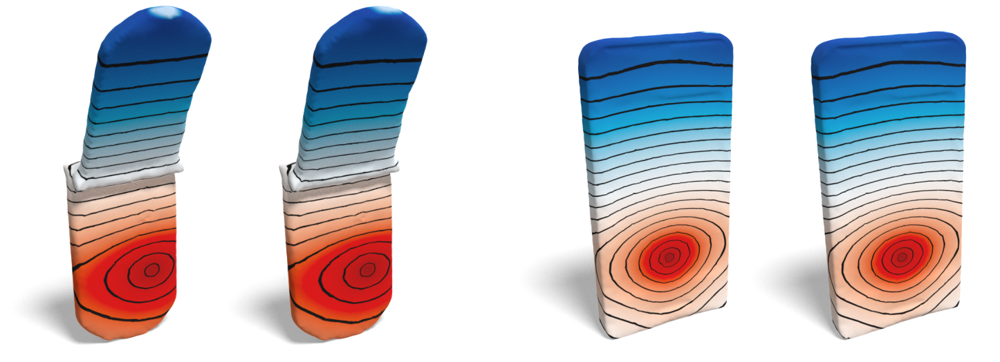
Figure 9. Train our network to predict the biharmonic distance. In each pair of results, the exact biharmonic distance is on the left, and the predicted biharmonic distance is on the right. Our model predicts the biharmonic distance with high accuracy.

Biharmonic Distance

In this experiment, we verify the versatility of our method on learning high-dimensional embeddings for the biharmonic distance (Lipman et al., 2010). We select 900 meshes from the training data and compute their ground-truth biharmonic distance. Then, we train the network in a similar way as learning the geodesic embedding. After training, we can also query the biharmonic distances between two arbitrary points, eliminating the requirements of estimating eigenvectors and solving linear systems in (Lipman et al., 2010). We show the predicted results in Fig. 9, which are faithful to the ground truth. Potentially, it is possible to apply our method to learn embeddings for other types of distances on manifolds, such as the diffusion distance (Coifman et al., 2005) and the earth mover’s distance (Solomon et al., 2014).

Finetune

We also test the effect of finetuning by additionally training the network with the ground-truth samples on the specified mesh to improve the performance of GeGnn. An example is shown in Fig. 10. The mesh is not contained in ShapeNet and has a relatively complicated topology. Our network produces moderately accurate results initially. After finetuning, the predicted geodesic distance is much closer to the ground truth.

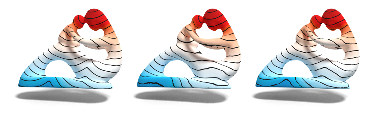
Figure 10. The effect of finetuning. Left: Exact geodesic distance. Middle: Predicted geodesic distance. Right: Predicted geodesic distance after 2,500 iterations of finetuning. Before finetuning, the MRE is 4.1%, while after finetuning, the MRE is reduced to 1.0%.

Scalability and Convergence

Our network is fully convolutional and has good scalability with large meshes. We firstly test our method on the ShapeNet-A dataset with meshes of different sizes. Specifically, we apply the Loop subdivision (Loop, 1987) on ShapeNet-A to get two sets of meshes with an average number of vertices of 18,708 and 23,681, respectively. Then, we test the speed and accuracy of our method on these meshes. The results are shown in Table 2. Although our network is trained on ShapeNet with an average number of vertices of 5,057, it can efficiently and accurately deal with mesh with many more vertices. To verify the ability of our method on even larger meshes, we conduct experiments on subdivided spheres following (Surazhsky et al., 2005). We report the accuracy and running time in Fig. 11. The mean, maximum, and minimum relative errors on meshes are almost constant on spheres with a wide range of resolutions. And the running time only increases slightly when the resolution increases since the network runs in parallel on GPUs. The results demonstrate that our algorithm exhibits good convergence in terms of mesh resolution.

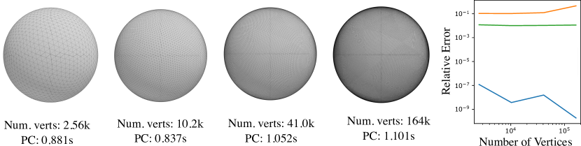
Figure 11. The convergence test. Left: The meshes with increasing number of vertices and their corresponding precomputation time. Right: The plot of mean (green), max (orange), and min (blue) relative error.

Table 2. The scalability test about the number of vertices. The “Ratio” represents the ratio between the average number of vertices of the test meshes and the average number of vertices in our training dataset.

Avg. Vert.	23682	18708	5202
Ratio	4.7	3.7	1.0
PC	0.1395s	0.1311s	0.089s
MRE	2.00%	1.88%	1.33%

4.2. Ablation Studies

In this section, we study and discuss the effectiveness of key designs in our method, including the graph convolution module, the graph pooling module, and the decoding function. We compare the MRE on the whole testing set, including 4,732 meshes.

Graph Convolution

The two key designs of our graph convolution are the local geometric features and the max aggregator in Eq. 4. To verify the effectiveness of these designs, we conduct a set of experiments to compare the performance; the mean relative errors are listed as follows:

	GeoConv	mean	sum	w/o dist	w/o rel. pos.
MRE	1.57%	2.53%	2.53%	1.67%	1.84%

After replacing the max aggregator with mean or sum, as shown in the third and fourth columns of the table, the performance drops by 0.96%. After removing the pairwise edge length (w/o dist) and the relative position (w/o rel. pos.), the performance drops by 0.27% and 0.67%, respectively.

We also compare our GeoConv with other graph convolutions, including GraphSAGE (Hamilton et al., 2017), GCN (Kipf and Welling, 2017), GATv2 (Brody et al., 2022), and EdgeConv (Wang et al., 2018). We keep all the other settings the same as our method, except that we halve the batch size GATv2 and EdgeConv; otherwise, the models will run out of GPU memory. The results are listed as follows:

	GeoConv	GraphSAGE	GCN	GATv2	EdgeConv
MRE	1.57%	2.84%	3.25%	2.34%	1.62%

It can be seen that although our GeoConv in Eq. 4 only contains two trainable weights, it still outperforms all the other graph convolutions by a large margin in the task of geodesic embedding. Our GeoConv is easy to implement and can be implemented within 15 lines of code with the Torch Geometric library (Fey and Lenssen, 2019), which we expect to be useful for other geometric learning tasks.

Graph Pooling

In this experiment, we replace our GeoPool with naive grid-based pooling to verify the efficacy of our graph pooling. We did not compare the pooling strategy in MeshCNN (Hanocka et al., 2019) and SubdivConv (Hu et al., 2022) since they require sequential operations on CPUs and are time-consuming for our task. The MRE of grid-based pooling is 2.04%, which is 0.47% worse than our GeoPool.

Decoding Function

In this experiment, we verify the superiority of our MLP-based function over conventional Euclidean distance (Panozzo et al., 2013; Xia et al., 2021) when decoding the geodesic distance from the embedding vectors. After replacing our MLP with Euclidean distance, the MRE is 3.03%, decreasing by 1.46%.

4.3. Applications

In this section, we demonstrate several interesting applications with our constant-time GDQs.

Texture Mapping

We create a local geodesic polar coordinate system around a specified point on the mesh, which is known as the logarithmic map in differential geometry, also called the logarithmic map. Then, we can map the texture from the polar coordinate system to the mesh. We follow (Xin et al., 2012; Panozzo et al., 2013) to compute the exponential map with constant-time GDQs, which has proven to be more efficient and more accurate than (Schmidt et al., 2006). The results are shown in Fig. 12, where the texture is smoothly mapped to curved meshes with the computed exponential map, demonstrating that our algorithm is robust even on the edge of the surface.

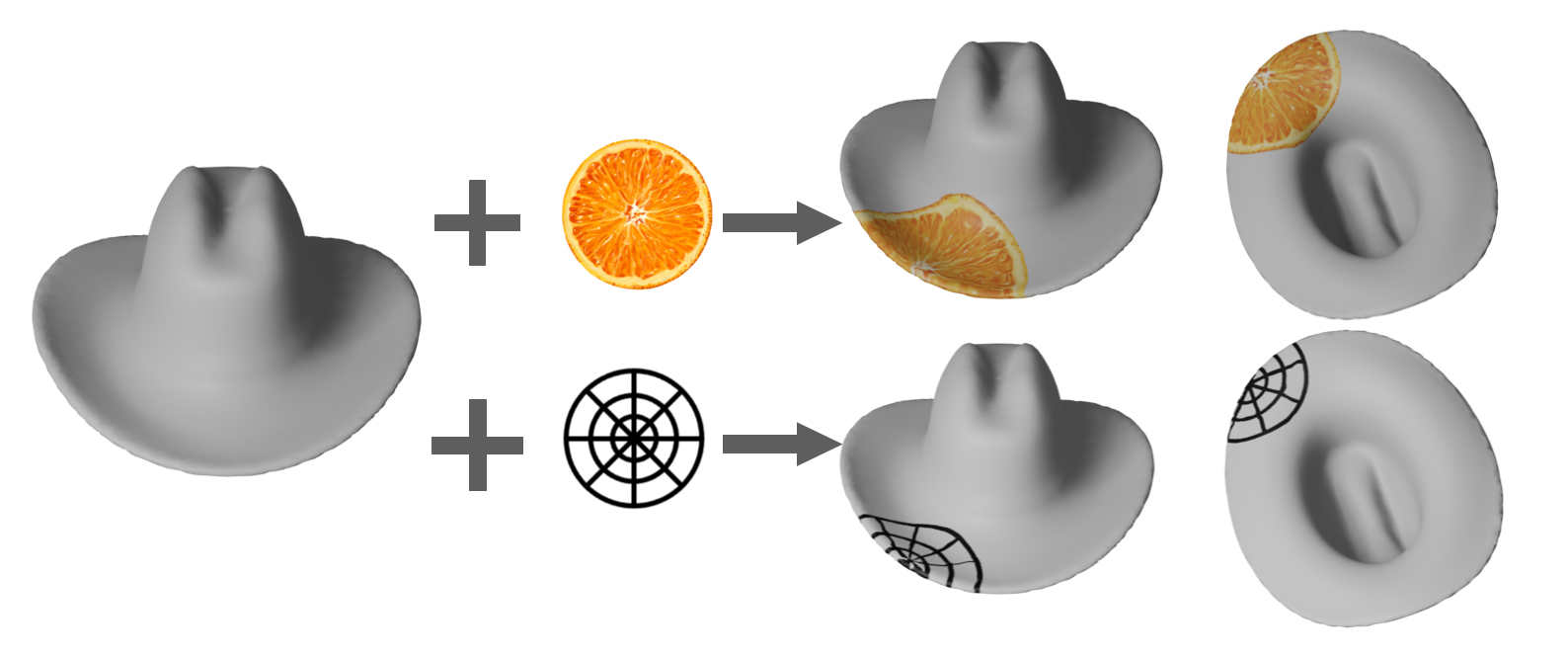
Figure 12. Texture Mapping. We compute the exponential map with our constant-time GDQs (below) and map the texture from the polar coordinate system to the mesh (top).

Shape Matching

Shape distributions (Osada et al., 2002) are widely used in shape matching and retrieval, which is based on shape histograms of pairwise distances between many point pairs on the mesh using a specific shape function. In (Osada et al., 2002), the shape function is defined as the Euclidean distance or angle difference between two points. We follow (Martinek et al., 2012) to use the geodesic distances as the shape function. Our constant-time GDQs allow for the extremely efficient computation of geodesic distances between randomly selected surface points. The results are shown in Fig. 13; we can see that the shape distributions computed with geodesic distances are invariant to the articulated deformation of the mesh, while the shape distributions computed with Euclidean distances are not.

Geodesic Path

We can also efficiently compute the geodesic path by tracing the gradient of the geodesic distance field from the target point to the source point (Xin et al., 2012; Kimmel and Sethian, 1998). The gradient of the geodesic distance field can be computed in constant time on each triangle with our method, therefore the geodesic path can be computed in $\mathcal{O}(k)$ time, where $k$ is the number of edges crossed by the path. The results are shown on the right. For visualization, the geodesic distance field is also drawn on the mesh.

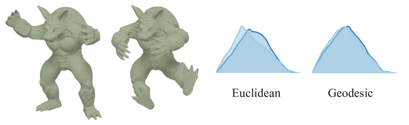
Figure 13. Shape distributions. We use Blender to deform the mesh of the armadillo and compute the shape distributions with geodesic distances and Euclidean distances as shape functions, respectively. The shape distributions computed with geodesic distances are more invariant to the articulated deformation of the mesh than Euclidean distances.

5. Discussion and limitations

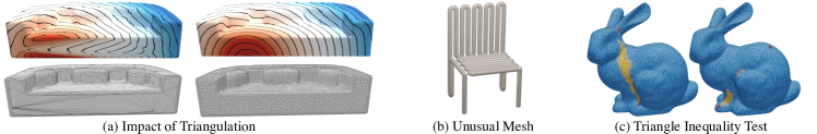
Figure 14. The limitations of our method. (a) Our method cannot handle the extremely anisotropic mesh; the result on a regular mesh is much better, as shown on the right. (b) Our method cannot handle shapes with unusual geometry. (c) Our method cannot guarantee the triangle inequality for the predicted geodesic distances. For fixed vertices marked in red, all vertices for which triangle inequality is not satisfied are marked in orange.

In this section, we discuss our method’s limitations and possible improvements.

Triangulations

Although our method exhibits good robustness against different triangulations, it cannot work well with extremely anisotropic meshes; an example is shown in Fig. 14-(a). However, this issue could be easily alleviated by making the mesh regular through remeshing.

Unusual meshes

Our method may struggle to process meshes that have unusual topology and geometry. The chair in Fig. 14-(b) is constructed by bending a long and thin tube multiple times; such geometry is rare in the training dataset. As a consequence, our method produces an MRE of about 25%, significantly higher than the average error throughout the test set. In order to address this issue, we could potentially expand and diversify our training data while also enlarging our networks to enhance the overall generalizability and robustness.

Triangle Inequality and Error Bound

The geodesic distance satisfies the triangle inequality. However, our GeGnn only predicts the approximate geodesic distances and cannot strictly pass the triangle inequality test. We follow (Solomon et al., 2014) to illustrate this issue in Fig. 14 (c). Specifically, given two fixed vertices $p$ and $q$, we identify and mark all vertices $x$ for which triangle inequality $d(p,q)\geq d(p,x)+d(q,x)$ are not satisfied. Our results are visually on par with the results of (Crane et al., 2013a). As a learning-based method, our GeGnn cannot offer theoretical guarantees of error bound, either. It would be interesting to incorporate additional geometric priors to address this limitation.

Rotation and Translation Invariance

Although the GeoConv in Eq. 4 is translation-invariant, the network is not due to the grid sampling in pooling. Our network is not rotation invariant, either. It is possible to leverage network architectures that possess invariant properties (Deng et al., 2021) to increase the performance further.

6. Conclusion

We propose to learn the geodesic embedding with graph neural networks, which enables constant time complexity for geodesic distance queries on discrete surfaces with arbitrary topology and geometry. We design a novel graph neural network to predict the vertex-wise geodesic embedding and leverage a lightweight MLP to decode the geodesic distance from the embeddings. The key technical contributions of our method include a novel graph convolution, graph pooling, and the design of the MLP decoder. We verify the efficiency, effectiveness, robustness, and generalizability of our method on ShapeNet and a variety of out-of-distribution meshes. We expect our work can inspire more learning-based methods for geodesic distance or general geometry problems. Several future works are discussed as follows.

General Geometric Distances

In this paper, we mainly use GeGnn to learn the geodesic embedding and verify the feasibility in learning an embedding for biharmonic distances. In the future, it is interesting to explore the possibility of learning other geometric distances and, furthermore, training a single general model for all geometric distances on meshes.

Geometry Optimization

The process of computing geodesic embedding is essentially a geometry optimization problem on meshes. In the future, we plan to use graph neural networks to solve other geometry optimization problems, such as shape deformation, remeshing, and parameterization.

Transformers on Meshes

Transformers have been prevailing in natural language processing and computer vision. It is interesting to use Transformers to meshes to replace the graph neural networks in our method for better performance in the future.

- (1)
- Adikusuma et al. (2020) Yohanes Yudhi Adikusuma, Zheng Fang, and Ying He. 2020. Fast construction of discrete geodesic graphs. ACM Trans. Graph. 39, 2 (2020).
- Bendels and Klein (2003) G. H. Bendels and R. Klein. 2003. Mesh Forging: Editing of 3D-Meshes Using Implicitly Defined Occluders. In SGP.
- Bhat et al. (2004) Pravin Bhat, Stephen Ingram, and Greg Turk. 2004. Geometric texture synthesis by example. In Symp. Geom. Proc.
- Brody et al. (2022) Shaked Brody, Uri Alon, and Eran Yahav. 2022. How Attentive are Graph Attention Networks?. In ICLR.
- Carroll and Arabie (1998) J. Douglas Carroll and Phipps Arabie. 1998. Multidimensional scaling. Measurement, judgment and decision making (1998).
- Chang et al. (2015) Angel X. Chang, Thomas Funkhouser, Leonidas J. Guibas, Pat Hanrahan, Qixing Huang, Zimo Li, Silvio Savarese, Manolis Savva, Shuran Song, Hao Su, Jianxiong Xiao, Li Yi, and Fisher Yu. 2015. ShapeNet: An information-rich 3D model repository. arXiv preprint arXiv:1512.03012 (2015).
- Chen and Han (1990) Jindong Chen and Yijie Han. 1990. Shortest paths on a polyhedron. In Proceedings of the sixth annual symposium on Computational geometry.
- Coifman et al. (2005) Ronald R Coifman, Stephane Lafon, Ann B Lee, Mauro Maggioni, Boaz Nadler, Frederick Warner, and Steven W Zucker. 2005. Geometric diffusions as a tool for harmonic analysis and structure definition of data: Diffusion maps. Proceedings of the national academy of sciences 102, 21 (2005).
- Crane et al. (2013a) Keenan Crane, Fernando de Goes, Mathieu Desbrun, and Peter Schröder. 2013a. Digital geometry processing with discrete exterior calculus. In ACM SIGGRAPH 2013 courses.
- Crane et al. (2020) Keenan Crane, Marco Livesu, Enrico Puppo, and Yipeng Qin. 2020. A survey of algorithms for geodesic paths and distances. arXiv preprint arXiv:2007.10430 (2020).
- Crane et al. (2013b) Keenan Crane, Clarisse Weischedel, and Max Wardetzky. 2013b. Geodesics in heat: A new approach to computing distance based on heat flow. ACM Trans. Graph. 32, 5 (2013).
- Crane et al. (2017) Keenan Crane, Clarisse Weischedel, and Max Wardetzky. 2017. The Heat Method for Distance Computation. Commun. ACM 60, 11 (2017).
- Deng et al. (2021) Congyue Deng, Or Litany, Yueqi Duan, Adrien Poulenard, Andrea Tagliasacchi, and Leonidas J Guibas. 2021. Vector neurons: A general framework for so (3)-equivariant networks. In CVPR.
- Fey and Lenssen (2019) Matthias Fey and Jan Eric Lenssen. 2019. Fast Graph Representation Learning with PyTorch Geometric. In ICLR Workshop.
- Fey et al. (2018) Matthias Fey, Jan Eric Lenssen, Frank Weichert, and Heinrich Müller. 2018. SplineCNN: Fast Geometric Deep Learning with Continuous B-Spline Kernels. In CVPR.
- Fouss et al. (2007) Francois Fouss, Alain Pirotte, Jean-Michel Renders, and Marco Saerens. 2007. Random-walk computation of similarities between nodes of a graph with application to collaborative recommendation. IEEE Transactions on knowledge and data engineering 19, 3 (2007).
- Garland and Heckbert (1997) Michael Garland and Paul S Heckbert. 1997. Surface simplification using quadric error metrics. In SIGGRAPH.
- Gilmer et al. (2017) Justin Gilmer, Samuel S Schoenholz, Patrick F Riley, Oriol Vinyals, and George E Dahl. 2017. Neural message passing for quantum chemistry. In ICML.
- Gotsman and Hormann (2022) Craig Gotsman and Kai Hormann. 2022. Compressing Geodesic Information for Fast Point-to-Point Geodesic Distance Queries. In SIGGRAPH Asia.
- Hamilton et al. (2017) Will Hamilton, Zhitao Ying, and Jure Leskovec. 2017. Inductive Representation Learning on Large Graphs. In NeurIPS.
- Hanocka et al. (2019) Rana Hanocka, Amir Hertz, Noa Fish, Raja Giryes, Shachar Fleishman, and Daniel Cohen-Or. 2019. MeshCNN: A network with an edge. ACM Trans. Graph. (SIGGRAPH) 38, 4 (2019).
- Hanocka et al. (2020) Rana Hanocka, Gal Metzer, Raja Giryes, and Daniel Cohen-Or. 2020. Point2Mesh: A Self-Prior for Deformable Meshes. ACM Trans. Graph. (SIGGRAPH) 39, 4 (2020).
- He et al. (2016) Kaiming He, Xiangyu Zhang, Shaoqing Ren, and Jian Sun. 2016. Deep residual learning for image recognition. In CVPR.
- Hoppe et al. (1993) Hugues Hoppe, Tony DeRose, Tom Duchamp, John McDonald, and Werner Stuetzle. 1993. Mesh optimization. In SIGGRAPH.
- Hu et al. (2020) Qingyong Hu, Bo Yang, Linhai Xie, Stefano Rosa, Yulan Guo, Zhihua Wang, Niki Trigoni, and Andrew Markham. 2020. RandLA-Net: Efficient Semantic Segmentation of Large-Scale Point Clouds. CVPR.
- Hu et al. (2022) Shi-Min Hu, Zheng-Ning Liu, Meng-Hao Guo, Jun-Xiong Cai, Jiahui Huang, Tai-Jiang Mu, and Ralph R Martin. 2022. Subdivision-based mesh convolution networks. ACM Trans. Graph. 41, 3 (2022).
- Kimmel and Sethian (1998) Ron Kimmel and James A. Sethian. 1998. Computing geodesic paths on manifolds. Proceedings of the National Academy of Science 95, 15 (1998).
- Kipf and Welling (2017) Thomas N Kipf and Max Welling. 2017. Semi-supervised classification with graph convolutional networks. In ICLR.
- Li et al. (2018) Yangyan Li, Rui Bu, Mingchao Sun, Wei Wu, Xinhan Di, and Baoquan Chen. 2018. PointCNN: Convolution on X-transformed points. In NeurIPS.
- Lipman et al. (2010) Yaron Lipman, Raif M Rustamov, and Thomas A Funkhouser. 2010. Biharmonic distance. ACM Trans. Graph. 29, 3 (2010).
- Liu et al. (2020) Hsueh-Ti Derek Liu, Vladimir G. Kim, Siddhartha Chaudhuri, Noam Aigerman, and Alec Jacobson. 2020. Neural Subdivision. ACM Trans. Graph. (SIGGRAPH) 39, 4 (2020).
- Loop (1987) Charles Loop. 1987. Smooth subdivision surfaces based on triangles. Thesis, University of Utah (1987).
- Loshchilov and Hutter (2019) Ilya Loshchilov and Frank Hutter. 2019. Decoupled weight decay regularization. In ICLR.
- Maehara (2013) Hiroshi Maehara. 2013. Euclidean embeddings of finite metric spaces. Discrete Mathematics 313, 23 (2013).
- Martinek et al. (2012) Michael Martinek, Matthias Ferstl, and Roberto Grosso. 2012. 3D Shape Matching based on Geodesic Distance Distributions. In Vision, Modeling and Visualization.
- Mémoli and Sapiro (2001) Facundo Mémoli and Guillermo Sapiro. 2001. Fast computation of weighted distance functions and geodesics on implicit hyper-surfaces. Journal of computational Physics 173, 2 (2001).
- Mémoli and Sapiro (2005) Facundo Mémoli and Guillermo Sapiro. 2005. Distance Functions and Geodesics on Submanifolds of and Point Clouds. SIAM J. Appl. Math. 65, 4 (2005).
- Mitchell et al. (1987) Joseph S. B. Mitchell, David M. Mount, and Christos H. Papadimitriou. 1987. The discrete geodesic problem. SIAM J. Comput. 16, 4 (1987).
- Osada et al. (2002) Robert Osada, Thomas Funkhouser, Bernard Chazelle, and David Dobkin. 2002. Shape distributions. ACM Trans. Graph. 21, 4 (2002).
- Panozzo et al. (2013) Daniele Panozzo, Ilya Baran, Olga Diamanti, and Olga Sorkine-Hornung. 2013. Weighted averages on surfaces. ACM Trans. Graph. (SIGGRAPH) 32, 4 (2013).
- Paszke et al. (2019) Adam Paszke, Sam Gross, Francisco Massa, Adam Lerer, James Bradbury, Gregory Chanan, Trevor Killeen, Zeming Lin, Natalia Gimelshein, Luca Antiga, Alban Desmaison, Andreas Kopf, Edward Yang, Zachary DeVito, Martin Raison, Alykhan Tejani, Sasank Chilamkurthy, Benoit Steiner, Lu Fang, Junjie Bai, and Soumith Chintala. 2019. PyTorch: An Imperative Style, High-Performance Deep Learning Library. In NeurIPS.
- Pfaff et al. (2020) Tobias Pfaff, Meire Fortunato, Alvaro Sanchez-Gonzalez, and Peter Battaglia. 2020. Learning Mesh-Based Simulation with Graph Networks. In ICLR.
- Pressley and Pressley (2010) Andrew Pressley and Andrew Pressley. 2010. Gauss’ theorema egregium. Elementary differential geometry (2010).
- Qi et al. (2017) Charles R. Qi, Li Yi, Hao Su, and Leonidas J. Guibas. 2017. PointNet++: Deep hierarchical feature learning on point sets in a metric space. In NeurIPS.
- Qin et al. (2016) Yipeng Qin, Xiaoguang Han, Hongchuan Yu, Yizhou Yu, and Jianjun Zhang. 2016. Fast and exact discrete geodesic computation based on triangle-oriented wavefront propagation. ACM Trans. Graph. (SIGGRAPH) 35, 4 (2016).
- Raviv et al. (2010) Dan Raviv, Alexander M Bronstein, Michael M Bronstein, and Ron Kimmel. 2010. Full and partial symmetries of non-rigid shapes. International Journal of Computer Vision 89, 1 (2010).
- Ronneberger et al. (2015) Olaf Ronneberger, Philipp Fischer, and Thomas Brox. 2015. U-Net: Convolutional networks for biomedical image segmentation. In International Conference on Medical image computing and computer-assisted intervention.
- Rustamov et al. (2009) Raif M Rustamov, Yaron Lipman, and Thomas Funkhouser. 2009. Interior distance using barycentric coordinates. Comput. Graph. Forum (SGP) 28, 5 (2009).
- Schmidt et al. (2006) Ryan Schmidt, Cindy Grimm, and Brian Wyvill. 2006. Interactive Decal Compositing with Discrete Exponential Maps. In SIGGRAPH.
- Sethian (1999) James A. Sethian. 1999. Fast marching methods. SIAM review 41, 2 (1999).
- Shamai et al. (2018) Gil Shamai, Michael Zibulevsky, and Ron Kimmel. 2018. Efficient inter-geodesic distance computation and fast classical scaling. TPAMI 42, 1 (2018).
- Sharp and Crane (2020) Nicholas Sharp and Keenan Crane. 2020. You can find geodesic paths in triangle meshes by just flipping edges. ACM Trans. Graph. (SIGGRAPH ASIA) 39, 6 (2020).
- Simonovsky and Komodakis (2017) Martin Simonovsky and Nikos Komodakis. 2017. Dynamic edge-conditioned filters in convolutional neural networks on graphs. In CVPR.
- Solomon et al. (2014) Justin Solomon, Raif Rustamov, Leonidas Guibas, and Adrian Butscher. 2014. Earth mover’s distances on discrete surfaces. ACM Trans. Graph. (SIGGRAPH) 33, 4 (2014).
- Surazhsky et al. (2005) Vitaly Surazhsky, Tatiana Surazhsky, Danil Kirsanov, Steven J Gortler, and Hugues Hoppe. 2005. Fast exact and approximate geodesics on meshes. ACM Trans. Graph. 24, 3 (2005).
- Tao et al. (2019) Jiong Tao, Juyong Zhang, Bailin Deng, Zheng Fang, Yue Peng, and Ying He. 2019. Parallel and scalable heat methods for geodesic distance computation. IEEE Trans. Pattern Anal. Mach. Intell. 43, 2 (2019).
- Thomas et al. (2019) Hugues Thomas, Charles R. Qi, Jean-Emmanuel Deschaud, Beatriz Marcotegui, François Goulette, and Leonidas J. Guibas. 2019. KPConv: Flexible and deformable convolution for point clouds. In ICCV.
- Tsitsiklis (1995) John N. Tsitsiklis. 1995. Efficient algorithms for globally optimal trajectories. IEEE transactions on Automatic Control 40, 9 (1995).
- Velickovic et al. (2017) Petar Velickovic, Guillem Cucurull, Arantxa Casanova, Adriana Romero, Pietro Lio, and Yoshua Bengio. 2017. Graph attention networks. stat 1050, 20 (2017).
- Wang et al. (2018) Nanyang Wang, Yinda Zhang, Zhuwen Li, Yanwei Fu, Wei Liu, and Yu-Gang Jiang. 2018. Pixel2Mesh: Generating 3D mesh models from single RGB images. In CVPR.
- Wang et al. (2022) Peng-Shuai Wang, Yang Liu, and Xin Tong. 2022. Dual Octree Graph Networks for Learning Adaptive Volumetric Shape Representations. ACM Trans. Graph. (SIGGRAPH) 41, 4 (2022).
- Wang et al. (2019) Yue Wang, Yongbin Sun, Ziwei Liu, Sanjay E Sarma, Michael M Bronstein, and Justin M Solomon. 2019. Dynamic graph CNN for learning on point clouds. ACM Trans. Graph. 38, 5 (2019).
- Weber et al. (2008) Ofir Weber, Yohai S Devir, Alexander M Bronstein, Michael M Bronstein, and Ron Kimmel. 2008. Parallel algorithms for approximation of distance maps on parametric surfaces. ACM Transactions on Graphics (TOG) (2008).
- Wu and He (2018) Yuxin Wu and Kaiming He. 2018. Group normalization. In ECCV.
- Wu et al. (2020) Zonghan Wu, Shirui Pan, Fengwen Chen, Guodong Long, Chengqi Zhang, and S Yu Philip. 2020. A comprehensive survey on graph neural networks. IEEE Transactions on Neural Networks and Learning Systems 32, 1 (2020).
- Xia et al. (2021) Qianwei Xia, Juyong Zhang, Zheng Fang, Jin Li, Mingyue Zhang, Bailin Deng, and Ying He. 2021. GeodesicEmbedding (GE): a high-dimensional embedding approach for fast geodesic distance queries. IEEE. T. Vis. Comput. Gr. (2021).
- Xin and Wang (2009) Shi-Qing Xin and Guo-Jin Wang. 2009. Improving Chen and Han’s algorithm on the discrete geodesic problem. ACM Trans. Graph. (SIGGRAPH) 28, 4 (2009).
- Xin et al. (2012) Shi-Qing Xin, Xiang Ying, and Ying He. 2012. Constant-time all-pairs geodesic distance query on triangle meshes. In I3D.
- Xu et al. (2015) Chunxu Xu, Tuanfeng Y Wang, Yong-Jin Liu, Ligang Liu, and Ying He. 2015. Fast wavefront propagation (FWP) for computing exact geodesic distances on meshes. IEEE. T. Vis. Comput. Gr. 21, 7 (2015).
- Xu et al. (2018b) Keyulu Xu, Weihua Hu, Jure Leskovec, and Stefanie Jegelka. 2018b. How powerful are graph neural networks? arXiv preprint arXiv:1810.00826 (2018).
- Xu et al. (2009) Kai Xu, Hao Zhang, Andrea Tagliasacchi, Ligang Liu, Guo Li, Min Meng, and Yueshan Xiong. 2009. Partial intrinsic reflectional symmetry of 3D shapes. In ACM Trans. Graph. (SIGGRAPH ASIA).
- Xu et al. (2018a) Yifan Xu, Tianqi Fan, Mingye Xu, Long Zeng, and Yu Qiao. 2018a. SpiderCNN: Deep Learning on Point Sets with Parameterized Convolutional Filters. In ECCV.
- Yen et al. (2007) Luh Yen, Francois Fouss, Christine Decaestecker, Pascal Francq, and Marco Saerens. 2007. Graph nodes clustering based on the commute-time kernel. In Advances in Knowledge Discovery and Data Mining.
- Yi et al. (2017) Li Yi, Hao Su, Xingwen Guo, and Leonidas J. Guibas. 2017. SyncSpecCNN: Synchronized spectral CNN for 3D shape segmentation. In CVPR.
- Ying et al. (2013) Xiang Ying, Xiaoning Wang, and Ying He. 2013. Saddle vertex graph (SVG) a novel solution to the discrete geodesic problem. ACM Trans. Graph. (SIGGRAPH ASIA) 32, 6 (2013).
- Ying et al. (2014) Xiang Ying, Shi-Qing Xin, and Ying He. 2014. Parallel Chen-Han (PCH) algorithm for discrete geodesics. ACM Trans. Graph. 33, 1 (2014).
- Zhang et al. (2023) Qijian Zhang, Junhui Hou, Yohanes Yudhi Adikusuma, Wenping Wang, and Ying He. 2023. NeuroGF: A Neural Representation for Fast Geodesic Distance and Path Queries. arXiv preprint arXiv:2306.00658 (2023).
- Zigelman et al. (2002) Gil Zigelman, Ron Kimmel, and Nahum Kiryati. 2002. Texture mapping using surface flattening via multidimensional scaling. IEEE. T. Vis. Comput. Gr. 8, 2 (2002).