Implications for the Explosion Mechanism of Type Ia Supernovae from their Late-time Spectra

Abstract

Late-time spectra of Type Ia supernovae (SNe Ia) are important in clarifying the physics of their explosions, as they provide key clues to the inner structure of the exploding white dwarfs. We examined late-time optical spectra of 36 SNe Ia, including blackfive from our own project (SNe 2019np, 2019ein, 2021hpr, 2021wuf, and 2022hrs), with phase coverage of $\sim 200$ to $\sim 400$ days after maximum light. At this late phase, the outer ejecta have become transparent and the features of inner iron-group elements emerge in the spectra. Based on multicomponent Gaussian fits and reasonable choices for the pseudocontinuum around Ni and Fe emission features, we get reliable estimates of the Ni to Fe ratio, which is sensitive to the explosion models of SNe Ia. Our results show that the majority (about black67%) of our SNe Ia are more consistent with the sub-Chandrasekhar-mass (i.e., double-detonation) model, although they could be affected by evolutionary or ionisation effects. Moreover, we find that the Si II $\lambda$6355 velocity measured around the time of maximum light tends to increase with the Ni to Fe ratio blackfor the subsample with either redshifted or blueshifted nebular velocities, suggesting that progenitor metallicity might play an important role in accounting for the observed velocity diversity of SNe Ia.

1 Introduction

It is widely accepted that thermonuclear explosions of carbon-oxygen (CO) white dwarfs (WDs) with masses close to the Chandrasekhar limit (Nomoto et al., 1997; Hillebrandt & Niemeyer, 2000; Maoz et al., 2014) produce Type Ia supernovae (SNe Ia; see, e.g., Filippenko 1997 for a review of supernova classification). However, the mechanism that triggers the explosion and drives the propagation of the burning front, together with the nature of the donor, still remain unclear. Different models (that probably yield multiple valid channels of the explosion) invoke for the mass donor a non-WD companion such as a red giant or a helium star (the “single-degenerate” channel; Whelan & Iben, 1973), or another WD (the “double-degenerate” channel; Iben & Tutukov, 1984; Webbink, 1984). Also, increasing attention is being paid to sub-Chandrasekhar-mass (sub-$M_{\rm Ch}$) models (Bildsten et al., 2007; Shen & Bildsten, 2009). In addition to the vast parameter space for the progenitor systems, since the spectral features of SNe Ia exhibit both intermediate-mass elements (IMEs, i.e., from Si to Ca) and iron-group elements (IGEs), a transition of the nuclear burning front from subsonic to supersonic phases is expected to take place. Various models are mainly differentiated by the mechanism that triggers the detonation, as follows.

(i) In WDs near $M_{\rm Ch}$, owing to the compressional heating, an initial burning starts as a subsonic deflagration near its mass centre. As the burning front propagates outward, some parts of the front would be accelerated due to the Rayleigh-Taylor (RT) instabilities. Subsequent transitions from the subsonic deflagration to the supersonic detonation would take place at the plume structures that develop (Gamezo et al., 2005; Seitenzahl et al., 2013). Such a later-ignited “delayed-detonation” (DDT) front will synthesise the remaining WD into IGE-dominated products.

(ii) In WDs below $M_{\rm Ch}$ (i.e., $\lesssim 1.2$ M_⊙), the detonation of the CO WD can be triggered by an initial instability-induced detonation of an accreted helium shell on top of the WD (the “double-detonation”; Sim et al., 2010; Shen et al., 2018; Townsley et al., 2019).

(iii) Based on the result of hydrodynamic simulations, dynamical procedures such as the merger or the head-on collision of a double WD binary would also be able to meet the criteria that detonate the merged WD (Raskin et al., 2009; Kushnir et al., 2013; Pakmor et al., 2013; Pakmor, 2017).

Because WDs are mostly electron-degenerate matter consisting of carbon and oxygen, all models that blow up the WD are anchored to the same network of nuclear reactions, which dominate the electromagnetic signatures of SNe Ia around their peak luminosity. Such a commonality thus lead to universal chemical compositions and energetics regardless of the model details. This also roughly explains why the photometric and spectroscopic evolution of SNe Ia around the time of maximum light can be well reproduced by a broad range of models.

When WDs explode as SNe Ia, the timescale of their photometric evolution is well correlated with its peak luminosity. Both quantities are determined by the content of the heavy elements synthesised during the explosion. The peak luminosities of SNe Ia, including the slowly-declining, hot, luminous SN 1991T-like or SN 1999aa-like objects, the rapidly-declining, cool, subluminous SN 1991bg-like objects, and the “Branch-normal" objects (Branch et al., 1993), show a prominent correlation with the post-peak decline rate ${\Delta}m_{15}(B)$, with brighter objects having smaller ${\Delta}m_{15}(B)$ (Phillips, 1993). This correlation has been dubbed the “Phillips relation." It serves as the basic recipe for the cosmological use of SNe Ia, and it is believed to be governed mainly by the amount of ⁵⁶Ni produced in the explosion (Hoeflich & Khokhlov, 1996). Moreover, there is increasing evidence showing that SN Ia peak luminosity is not parameterised only by the decline rate. The inclusion of a color parameter helps tighten the dispersion of normalised peak luminosity (Tripp, 1998; Wang et al., 2005) and improves distance estimates from SNe Ia (e.g., Guy et al. 2007; Betoule et al. 2014).

However, despite the first-order simplicity and commonality of SNe Ia, diversity among a range of subtypes has also been explored by various studies. For example, Benetti et al. (2005) found that SNe Ia exhibit large scatter in the velocity evolution of the ejecta, and the velocity gradient measured from Si II $\lambda$6355 absorption is not correlated with $\Delta m_{15}(B)$ for Branch-normal SNe Ia. Wang et al. (2009b) divided Branch-normal SNe Ia into two groups based on Si II $\lambda$6355 velocities measured around their time of $B$-band maximum light, with the high-velocity (HV) group having Si velocities $\gtrsim 12,000$ $\rm km\ s^{-1}$ and the normal-velocity (NV) group having Si velocities $\lesssim 12,000$ $\rm km\ s^{-1}$. Such velocity diversity is independent of ${\Delta}m_{15}(B)$, and the origin of the spectral differences was interpreted as a geometric viewing-angle effect (Maeda et al., 2010a; Silverman et al., 2013). However, Wang et al. (2013) studied the birthplace environments of SNe Ia and found that HV SNe Ia tend to occur in inner, brighter regions of more-massive galaxies compared with the NV counterparts, suggesting that these two subclasses may have different progenitor properties. For example, HV SNe Ia are likely associated with metal-rich progenitors (Pan et al., 2015a; Pan, 2020), and they have more circumstellar matter (CSM) than NV SNe Ia (Wang et al., 2019). Thus, the idea that all SNe Ia originate from one family or one explosion mechanism is challenged even if we do not consider peculiar subclasses of SNe Ia such as those defined by subluminous SN 1991bg-like (Filippenko et al., 1992), overluminous SN 1991T-like (Phillips et al., 1992), SN 2002es-like (Ganeshalingam et al., 2012), and SN 2009dc-like (Silverman et al., 2011) SNe Ia.

To further explore the explosion mechanism and progenitor physics of SNe Ia, we need to inspect the inner regions of their ejecta. At early times, the outer ejecta are opaque, and the deeper regions are hidden. At a phase of over 200 days after peak brightness, the ejecta have expanded substantially and become transparent to the radiation from the inner core, which is dominated by emission from the Fe-group elements. At such nebular phases, the shape of the spectral profile over the wavelength range of 6800–7800 Å, dominated by [Fe II] and [Ni II] features (Maguire et al., 2018; Flörs et al., 2020), delivers critical constraints on the structure and abundance ratio of the Fe-group elements. For instance, the nonzero velocity shifts of [Fe II] and [Ni II] features indicate an asymmetric explosion (Maeda et al., 2010b). In addition, the iron is mainly contributed by the end product of the radioactive decay of ⁵⁶Ni, and the stable nickel was synthesised by the explosion. Thus, the Ni/Fe ratio in the nebular phase reflects the ratio of stable to radioactive isotopes of Fe-group elements produced in the explosion, which is sensitive to the central density of the exploding WD. Maguire et al. (2018) used a multicomponent Gaussian fit to measure the Ni/Fe ratio in the 7300 Å region in optical spectra to distinguish $M_{\rm Ch}$ and sub-$M_{\rm Ch}$ models since the central densities of WDs are quite different for these two explosion models. Flörs et al. (2020) and Graham et al. (2022) also measured the Ni/Fe ratio using different methods, but their results were generally lower than those given by Maguire et al. (2018). Flörs et al. (2020) mentioned that the differences are mainly due to the placement of the pseudocontinuum across the 7300 Å region. In this work, we generally follow the fitting method of Maguire et al. (2018) but adopt the pseudocontinuum blackin a different way.

Using nebular-phase spectra of SNe Ia published in the literature as well as data collected through our own program, we attempt to provide more-accurate measurements of the Ni/Fe ratio to put tighter constraints on the explosion mechanism of SNe Ia. Since the Ni/Fe ratio can be affected by the progenitor metallicity (Timmes et al., 2003; Shen et al., 2018; Shingles et al., 2020), we also examine correlations of this ratio with SN Ia observables measured at early times, such as the Si II velocity and $\Delta m_{15}(B)$.

The paper is structured as follows. We outline the sample used in our analysis in Section 2, and Section 3 shows the fitting methods. Our results are presented in Section 4 and discussed in Section 5. Section 6 summarises our conclusions.

2 Data Sources

In order to examine the distribution of the Ni/Fe ratio, we collect a sample of 58 late-time spectra taken at $t\approx+200$–400 days after maximum light for 36 SNe Ia. Those showing peculiar properties such as SN 1991T-like and SN 1991bg-like SNe Ia are also included except when their spectra exhibit strong calcium features or have a flat profile in the 7300 Å region. The publicly available data were retrieved using the Open Supernova Catalog (OSC; Guillochon et al. 2017), the Weizmann Interactive Supernova data REPository (WISeREP; Yaron & Gal-Yam 2012), and the Supernovae Database (SNDB; Silverman et al. 2012a; Shivvers et al. 2019). The $t\approx+384$ day spectrum of SN 2017fgc comes from Zeng et al. (2021). Information on the spectra collected by our own project is presented in Section 2.1. An overview of the observations for all the SNe Ia in this work is listed in Table 2. References for all the late-time spectra can be found in Table 3.

To study the connections between early-time and late-time properties, blackwe used the spectrum around the time of maximum light (i.e., within about 3 days from the $B$-band peak, except for SN 2012hr at +5 days and ASASSN-14jg at +6 days) to measure the Si II $\lambda$6355 velocity from the absorption minimum for each object of our sample. The Si velocities and the phase of the spectra used in the measurements are presented in Table 2. We collected the post-peak decline rate ${\Delta}m_{15}(B)$ and the date of $B$-band maximum from the literature when available. For SNe 2003kf, 2012hr, and 2013cs, these two parameters are estimated by applying the SALT2 (Guy et al., 2007) fit to their light curves. All spectra used in the analysis have been corrected for host-galaxy redshift from the NASA/IPAC Extragalactic Database (NED) and extinction due to the Milky Way black(Schlafly & Finkbeiner, 2011) and host galaxy whenever possible (for details, see Table 2). As we only focus on the 7300 Å region in the spectra, the results should suffer little from uncertainties in extinction corrections.

2.1 Late-Time Spectra from our Project

Our program aims to collect some late-time spectra for SNe Ia that were well observed at early phases. Thus far, we have obtained late-time spectra of SN 2019np (Sai et al., 2022), SN 2019ein (Xi et al., 2022), SN 2021hpr (Iskandar et al., in prep.), SN 2021wuf (Zeng et al., in prep.), and SN 2022hrs (Liu et al., in prep.). The nebular spectra of these last four SNe Ia were taken with LRIS (Oke et al., 1995) mounted on the 10 m Keck-I telescope and the DEIMOS spectrograph (Faber et al., 2003) on the 10 m Keck-II telescope on Maunakea, and the Kast double spectrograph (Miller & Stone, 1993) mounted on the Shane 3 m telescope at Lick Observatory. The late-time spectra of SN 2019np were obtained with OSIRIS mounted on the 10.4 m Gran Telescopio CANARIAS (GTC) at the Roque de Los Muchachos Observatory (Spain). blackTo minimise slit losses caused by atmospheric dispersion (Filippenko, 1982), the slit was oriented at or near the parallactic angle. The Keck I/LRIS spectra were reduced using the LPipe pipeline (Perley, 2019). The GTC/OSIRIS, Keck II/DEIMOS, and Shane/Kast observations were reduced using standard IRAF routines for CCD processing (e.g., Silverman et al. 2012a) and optimal spectrum extraction (Horne, 1986). The spectra were flux calibrated using observations of appropriate spectrophotometric standard stars observed on the same night, at similar airmasses, and with an identical instrument configuration. We corrected for the atmospheric extinction using the extinction curves of local observatories. A journal of observations is given in Table 1 and the corresponding spectra are shown in Fig. 1.

Table 1: Overview of the Observations.

Name	Observation	Observation	Phase	Range	Instrument	Telescope	Exposure
	MJD	Date (UTC)	(d)	[Å]			[s]
SN 2019ein	58932	2020 Mar. 24	+313	3147–10,278	LRIS	Keck I	1077.5
SN 2019np	58813	2019 Nov. 26	+303	3812–7830	OSIRIS	GTC	1380
SN 2019np	58878	2020 Jan. 30	+368	3832–7831	OSIRIS	GTC	1380
SN 2021hpr	59585	2022 Jan. 6	+263	3622–10,380	Kast	Shane	3600
SN 2021hpr	59610	2022 Jan. 31	+288	3166–10,275	LRIS	Keck I	1200
SN 2021wuf	59670	2022 Apr. 1	+208	3142–10,272	LRIS	Keck I	1200
SN 2021wuf	59761	2022 July 1	+299	3138–10,259	LRIS	Keck I	2400
SN 2022hrs	59995	2023 Feb. 20	+297	3634–10,752	Kast	Shane	3660
SN 2022hrs	60025	2023 Mar. 22	+327	4420–9626	DEIMOS	Keck II	1500

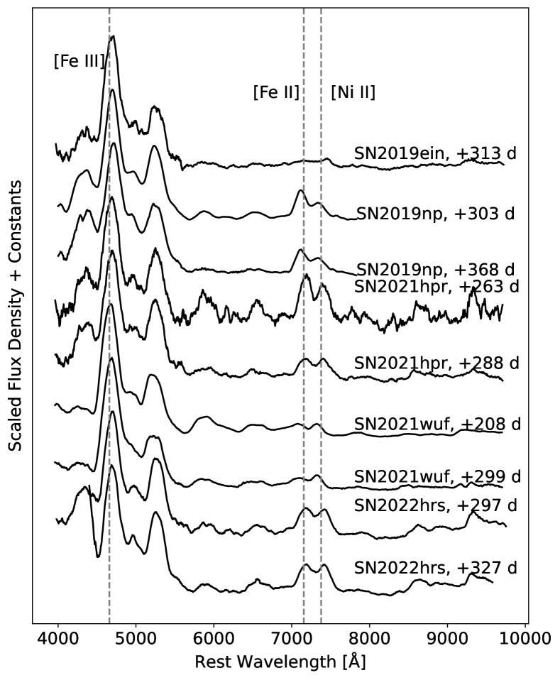
Figure 1: Late-time spectra of SNe 2019ein, 2019np, 2021hpr, 2021wuf, and 2022hrs. Flux densities ($f_{\lambda}$) are all normalised to the [Fe III] 4700 Å feature black and smoothed with a Savitsky-Golay filter of width $\sim 50$ Å and order 1. The rest-frame wavelengths of [Fe III] 4659 Å, [Fe II] 7155 Å, and [Ni II] 7378 Å are marked by dashed lines.

3 Fitting Method

3.1 Multicomponent Gaussian Fit

To derive the Ni/Fe ratio in an SN Ia explosion, we focus on the 7300 Å region in the nebular-phase spectra, where the emission features are dominated by [Fe II] (7155, 7172, 7388, 7453 Å) and [Ni II] (7378, 7412 Å) (Maguire et al., 2018). The [Fe II] features mainly come from ⁵⁶Fe which results from the decay of ⁵⁶Co, while the [Ni II] features are mostly contributed by stable ⁵⁸Ni, since radioactive ⁵⁶Ni has a half-life of only 6.1 days and its contribution is negligible at late times.

To measure accurately the velocity shift, width, and strength of the above features, a multicomponent Gaussian function is used to fit the line profiles following Maguire et al. (2018),

$$f(\lambda)=\sum_{i=1}^{6}A_{i}{\rm exp}(-\frac{(\lambda-\lambda_{i}^{\rm centre})^{2}}{2\sigma_{i}^{2}})\,,$$ (1)

where $A_{i}$ is the strength of the emission feature, $\lambda_{i}^{\rm centre}$ is the central wavelength, and $\sigma_{i}$ represents the width. The subscript $i$ denotes different components. With these parameters, we can calculate the velocity shift ($v_{i}$), full width at half-maximum intensity ($\rm FWHM_{i}$), and flux ($F_{i}$) for different emission components:

$$v_{i}=(\frac{\lambda_{i}^{\rm centre})^{2}-(\lambda_{i}^{\rm rest})^{2}}{\lambda_{i}^{\rm centre})^{2}+(\lambda_{i}^{\rm rest})^{2}}c\,,$$ (2)

$${\rm FWHM_{i}}=\frac{(\sqrt{2\,{\rm ln}\,2}\sigma_{i}+\lambda_{i}^{\rm rest})^{2}-(\lambda_{i}^{\rm rest})^{2}}{(\sqrt{2\,{\rm ln}\,2}\sigma_{i}+\lambda_{i}^{\rm rest})^{2}+(\lambda_{i}^{\rm rest})^{2}}2c\,,$$ (3)

$${\rm and}~{}F_{i}=\sqrt{2\pi}A_{i}\sigma_{i}\,,$$ (4)

where $\lambda_{i}^{\rm rest}$ is the rest-frame wavelength of the corresponding emission component and $c$ is the speed of light, blackand we use the relativistic Doppler formula to convert wavelengths to velocities. The Ni/Fe ratio is inferred from the flux ratio of [Ni II] 7378 Å and [Fe II] 7155 Å, $F_{7378}/F_{7155}$; more details are presented in Section 4.2.

Before fitting the Ni and Fe emission features, each spectrum blackis smoothed with a Savitsky-Golay filter of width $\sim 20$–50 Å and order 1 using the scipy package’s $\rm signal.savgol\_filter$ function. The pseudocontinuum is defined as a straight line connecting the interactively chosen points to the red and blue of the features in the 7300 Å region. We notice that the red side of the features near 7600 Å were often affected by telluric absorption lines, so we choose a region longward of this (i.e., at $\sim 7700$ Å) as the red continuum point when such absorption appears in the spectrum, and we mask the absorption before fitting. blackAfter subtracting the pseudocontinuum, we apply a multicomponent Gaussian function to fit the observed features. Following Maguire et al. (2018), line widths and velocity shifts of the same species are set to the same values, and the relative strengths of the same species are fixed as well. Following Jerkstrand et al. (2015), the strengths of the [Fe II] 7172, 7388, and 7453 Å features relative to [Fe II] 7155 Å are set to 0.24, 0.19, and 0.31, respectively, while the [Ni II] 7412 Å feature has a relative strength of 0.31 compared to [Ni II] 7378 Å. Thus, there are only six free parameters for the multicomponent Gaussian function: width, velocity shift, and strength of each of [Fe II] 7155 Å and [Ni II] 7378 Å. Similar to Graham et al. (2022), we also place the boundary of the nickel width to be $\lesssim 13,000$ km s^-1.

blackIt should be noted that possible [Ca II] emission at 7291.5 and 7323.9 Å could contaminate the late-time spectra. We try to add two additional Gaussian components to represent the weak [Ca II] emission lines in the fit, where the velocity shifts of the [Fe II] and [Ni II] are set to the same values; otherwise the [Ca II] could dominate the blue or red peak. We find that the influence of the [Ca II] emission on our fitting is very limited for most objects except the SN 1991bg-like SNe Ia such as SN 1986G and SN 2003gs, blackwhich is consistent with previous work (e.g., Graham et al. 2017; Maguire et al. 2018; Flörs et al. 2020; Tucker et al. 2022). In fact, the spectra of SN 1986G and SN 2003gs cannot be fit well by only [Fe II] and [Ni II], so we fit them by adding the [Ca II] emission lines.

To estimate the uncertainties, blackthe endpoints of the continuum vary within 10–50 Å (smaller variation ranges for lower-quality spectra to avoid improperly determining of the continuum; if some regions are masked, their edges are varied within 10 Å) and the emission features at 7100–7400 Å are refit 1000 times through the Monte Carlo method. A fit is rejected when the FWHM of nickel emission features is $>12,500$ km s^-1. The standard deviation in the measurement is taken as one part of the uncertainty of the Gaussian parameters. Additional uncertainty comes from smoothing the spectrum, which is taken as the difference between the results given by the smoothed spectrum and the observed one. Following Maguire et al. (2018), an uncertainty of 200 $\rm km\ s^{-1}$ is added to the velocity-shift measurement to account for the peculiar velocities of host galaxies.

Graham et al. (2022) also adopted the analysis method of Maguire et al. (2018) to fit the 7300 Å region, finding that the nickel line profile can be unusually broad. Thus, they proposed a two-stage minimum-Ni fit to further suppress the nickel contribution, which led to a lower Ni/Fe ratio. Flörs et al. (2020) used a non-local-thermodynamic-equilibrium (NLTE) level population model of the first and second ionisation stages of iron, nickel, and cobalt to fit the full late-time spectra for their SN Ia sample. The Ni/Fe ratios derived by them are lower than those obtained by Maguire et al. (2018) for the same objects and the deviations were attributed to the placement of the pseudocontinuum. Although in this work we mainly follow the fitting method of Maguire et al. (2018), we try to give a more reasonable placement of the pseudocontinuum to make the Ni/Fe ratio more accurate; see Section 3.2.

3.2 Selection of Pseudocontinuum

We notice that there exists a small bump at 6800–7000 Å in most spectra of our sample, which tends to disappear at later phases and might be contributed by Co lines such as [Co III] $\lambda$6855 (Flörs et al., 2020). In the analysis by Maguire et al. (2018), the blue end of the continuum for the emission features near 7100–7400 Å was chosen as the point around 6900 Å (called point $A^{\prime}$), which would induce a steeper pseudocontinuum. In our analysis, we prefer to choose the minimum in the blue wing of the bump as the blue end of the continuum (called point $A$) to place a flatter pseudocontinuum. Fig. 2 shows a comparison of these two placements for spectra of SN 2011fe and SN 2012fr, two well-observed nearby SNe Ia (e.g., Zhang et al. 2016; Childress et al. 2015). The pseudocontinuum defined with point $A^{\prime}$ is steeper than that defined with point $A$, significantly affecting the fitting results. In the following analysis, we call these two cases of choosing the blue side of the continuum as case $A$ and case $A^{\prime}$, respectively.

blackWe mask the bump feature at 6800–7000 Å before fitting. However, this bump may be blended with iron emission [Fe II] 7155 Å. To roughly estimate the influence on the fitting, we blacktry to use another Gaussian component to fit the bump feature near 6900 Å instead of masking it. We find that the $F_{7378}/F_{7155}$ ratio derived by these two methods can differ by about 15% when using the $t\approx+222$ day spectrum of SN 2012fr. Such a discrepancy becomes less significant with time, and it nearly disappears in the $t\approx+357$ day spectrum of SN 2012fr. Assuming that the bump feature near 6900 Å is indeed mainly contributed by [Co III] 6855 Å, it has a limited effect on the iron feature unless the [Co III] emission has an unreasonably broad width.

An important reason for us to choose case $A$ is that it gives a smaller systematic error for the estimation of feature velocities. Assuming that velocities of [Fe II] 7155 Å and [Ni II] 7378 Å are similar (Maeda et al., 2010b), the velocity difference of these two features should be close to zero or at least has a symmetric distribution with respect to zero for our sample. Fig. 3 compares the velocity fitting results between case $A$ and case $A^{\prime}$. We find that the velocity difference of case $A^{\prime}$ with a mean value of $\sim-900$ km s^-1 tends to be bluer — blackthat is, the nickel velocity tends to be bluer than the iron velocity. This bias is more serious for the spectra taken at $t<+300$ days. Meanwhile, the velocity difference distribution of case $A$ is consistent with our expectations, with a mean value of $\sim-200$ km s^-1, close to zero.

Another problem of case $A^{\prime}$ is the overly broad nickel component in some fitting cases, which is also mentioned by Graham et al. (2022). We find that, in most cases, the unreasonably broad nickel component can be avoided by using point $A$ to set the pseudocontinuum and adjusting the masking regions. When the adjustment doesn’t work (only for the spectrum of SN 2017cbv at +317 days in our sample), we assume that the velocity shifts of [Fe II] and [Ni II] are the same, which can also avoid the overly broad nickel.

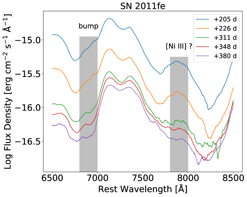
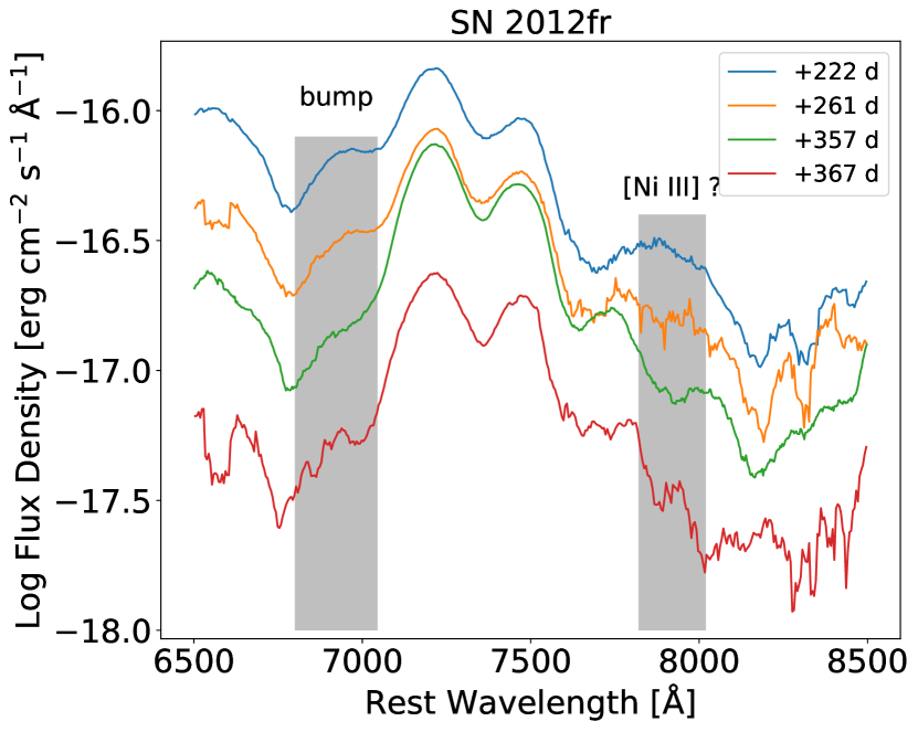
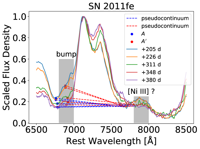
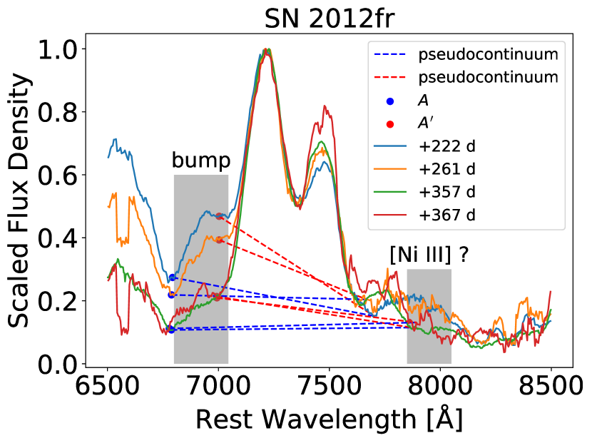
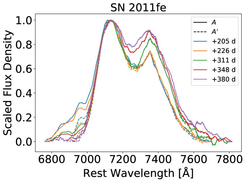
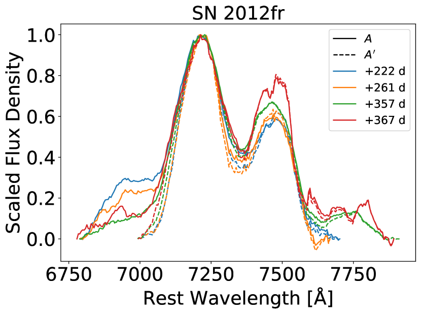
Figure 2: Evolution of the 7300 Å region shown for late-time spectra of SN 2011fe and SN 2012fr. blackAll spectra have been smoothed with a Savitsky-Golay filter of width $\sim 50$ Å and order 1. Upper panel: Evolution of unscaled spectra. Middle panel: Evolution of spectra scaled to the 7155 Å peak. The pseudocontinuum is defined as a straight line connecting the red and blue endpoints of the fitting region. The pseudocontinuum with point $A^{\prime}$ or point $A$ as the blue endpoint are shown with red and blue dashed lines, respectively. The bump near 6900 Å affecting the definition of the pseudocontinuum blackand the region near 7900 Å which might be contaminated by [Ni III] are labeled by the shaded region. blackBottom panel: Evolution of spectra from which the pseudocontinuum defined in the middle panel has been subtracted. The spectra obtained by subtracting the pseudocontinuum defined by $A$ or $A^{\prime}$ are shown as solid and dashed, respectively.

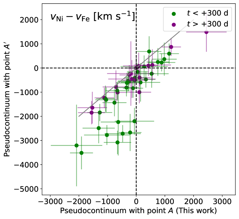
Figure 3: Comparisons of the velocity difference of [Ni II] 7378 Å and [Fe II] 7155 Å between case $A$ and case $A^{\prime}$. The velocity difference inferred from the spectra taken at $t<+300$ days are shown with green dots while those taken at $t>+300$ days are shown with purple dots.

blackFig. 4 shows the best fit to the 7300 Å region for the late-time spectra of SNe 2017fgc, 2019ein, 2019np, 2021hpr, 2021wuf, and 2022hrs.

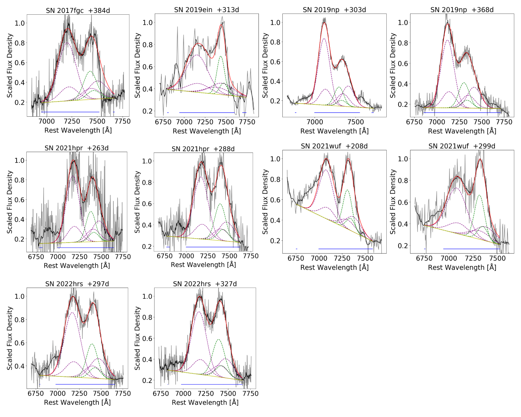
Figure 4: Best fits to the 7300 Å region dominated by [Fe II] and [Ni II] features. The reddening-corrected spectra are shown in grey while the smoothed spectra are in black. The overall fits are shown with a red line, while the fitting regions are indicated by blue lines. The [Fe II] and [Ni II] features are represented by purple and green dashed lines, respectively.

4 Results

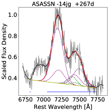
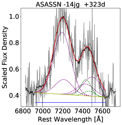
Figure 10: Best fits to the 7300 Å region dominated by [Fe II] and [Ni II] features. The reddening-corrected spectra are shown in grey while the smoothed spectra are shown in black. The overall fits are shown in red, the [Fe II] features are in purple dashed lines, and the [Ni II] features are in green dashed lines. The [Ca II] features for SN 1986G and SN 2003gs are in pink. The fitting regions are indicated with blue lines, and the pseudocontinuum is in yellow.

The velocity shifts and line widths (i.e., FWHM) of the [Fe II] 7155 Å and [Ni II] 7378 Å features as well as their flux ratios are listed in Table 3. blackSignificant differences are found to exist in the velocity shifts and FWHM between the [Fe II] 7155 Å and [Ni II] 7378 Å features for some objects, as discussed in 4.1. We use the velocity shifts of [Fe II] 7155 Å and [Ni II] 7378 Å to identify whether the nebular velocities are redshifted or blueshifted, which might have a connection with asymmetric explosion models (Maeda et al., 2010a). We then use the flux ratio of [Fe II] 7155 Å and [Ni II] 7378 Å to roughly estimate the Ni/Fe ratio and constrain the explosion models. The fits for all the spectra used in this work are shown in Fig 10. The inferred nebular velocities and Ni/Fe ratios are also listed in Table 3. Some potential correlations can be found between nebular velocities, Ni/Fe ratios, Si II velocities at maximum light, and post-maximum decline rates $\Delta m_{15}(B)$.

4.1 blackVelocities and Widths of [Fe II] and [Ni II] features

blackNebular velocities were often estimated from the mean velocity shift inferred from the [Fe II] 7155 Å and [Ni II] 7378 Å emission features (e.g., Maeda et al. 2010a; Silverman et al. 2013). However, we note that the velocities inferred from [Fe II] and [Ni II] lines tend to show noticeable differences (e.g., over 1000 km s^-1) when their emission peaks are not of comparable strength. The velocity inferred from the weaker feature usually has a larger uncertainty relative to the stronger one. To quantify the difference between these two velocities, we apply a simple linear fit and find that $v_{\rm Ni}=1.24\,v_{\rm Fe}-170$ km s^-1. For an absolute mean velocity of $v_{\rm Fe}=1260$ km s^-1, the difference in $v_{\rm Ni}$ and $v_{\rm Fe}$ is within about 500 km s^-1, which is not significant. As the [Fe II] 7155 Å feature is usually stronger and has smaller measurement uncertainties in our sample, we adopt the [Fe II] velocity to represent the nebular velocity except when the [Ni II] 7378 Å feature is stronger. In these cases, we use the [Ni II] velocity to represent the nebular velocity (e.g., for SN 2003hv).

Fig. 5 shows the nebular velocities inferred from the [Fe II] 7155 Å blackor [Ni II] 7378 Å features in spectra taken at different phases. As can be seen, the nebular velocity does not show significant evolution in a given object. When the nebular velocity is close to zero within the quoted uncertainty, we consider its nebular velocity as zero instead of identifying it as a redshifted or blueshifted subclass. Among the 36 SNe Ia collected in our study, we find that 14 can be classified as having redshifted nebular velocities and 18 as having blueshifted ones. The numbers of redshifted and blueshifted objects are comparable, and the nebular velocities have a roughly symmetric distribution in the approximate range $-3000$ to 3000 km s^-1.

blackFor the line widths, there is considerable scatter between the FWHM of [Fe II] and [Ni II] features. The [Fe II] FWHM is usually larger than the [Ni II] FWHM, with mean values of $8429\pm 961$ km s^-1 and $6078\pm 1445$ km s^-1 (respectively) — approximately consistent with the DDT models of Seitenzahl et al. (2013) where ⁵⁶Ni usually has a slightly wider distribution than ⁵⁸Ni (see their Fig. 8). But in some extreme cases, the [Fe II] FWHM is much larger than the [Ni II] FWHM (e.g., more than a factor of two), not expected from the models. Note that the difference between [Fe II] and [Ni II] FWHM evolves with phase, with a tendency of being larger at earlier nebular phases (e.g., ASASSN-14jg), which can partially explain the large FWHM differences as revealed in Table A2. Nevertheless, inspecting the measurements for those spectra taken at similar phases (i.e., $t\approx 250$ days), we still find large FWHM scatter between [Ni II] and [Fe II] lines, suggesting that this scatter might be genuine and its origin should be further explored.

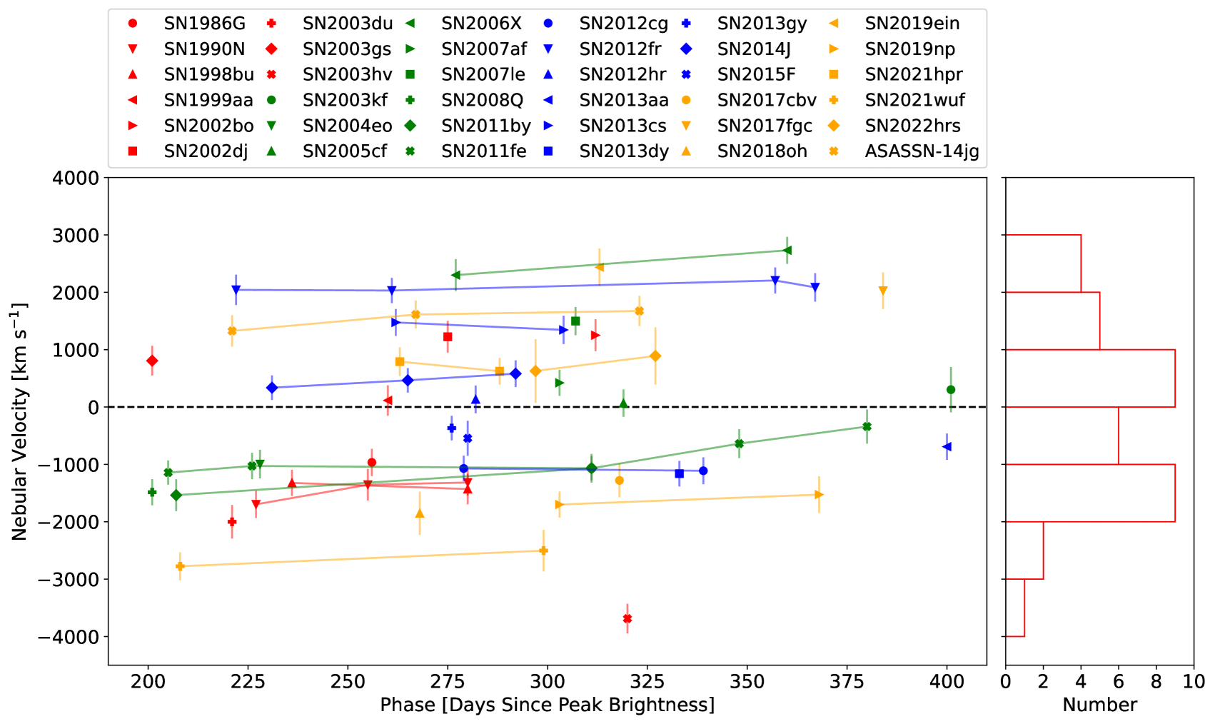
Figure 5: blackLeft panel: Nebular velocities inferred from the [Fe II] 7155 Å or [Ni II] 7378 Å features as a function of time. Right panel: The corresponding histogram for average nebular velocity measured for our sample.

4.2 Estimation of Ni/Fe Ratio

The Ni/Fe ratio is estimated following the method of Maguire et al. (2018),

$$\frac{n_{\rm Ni~{}II}}{n_{\rm Fe~{}II}\ }=\frac{L_{7378}}{L_{7155}}\exp{\left(-\frac{0.28}{kT}\right)}\frac{d_{C_{\rm Fe~{}II}}}{d_{C_{\rm Ni~{}II}}}/4.9\,,$$ (5)

where $d_{C_{\rm Fe~{}II}}/d_{C_{\rm Ni~{}II}}$ denotes the ratio of departure coefficients, $k$ is the Boltzmann constant blackin units of eV per K, and $T$ is the temperature. $L_{7378}/L_{7155}$ represents the luminosity ratio and is estimated as the measured flux ratio of [Fe II] 7155 Å and [Ni II] 7378 Å. Note that Maguire et al. (2018) used the ratio of pseudoequivalent width of these two lines.

To obtain a rough estimate of the Ni/Fe ratio, Maguire et al. (2018) adopted the value of the ratio of departure coefficients, temperature, and ionisation balance from a day 330 W7 model of Fransson & Jerkstrand (2015). The ratio $d_{C_{\rm Fe~{}II}}/d_{C_{\rm Ni~{}II}}$ has a range of 1.2–2.4 over the phase of interest, with smaller coefficients at earlier times when the conditions are slightly closer to LTE. The temperature is assumed to range from 3000 K to 8000 K, while the Ni/Fe ratio $n_{\rm Ni}/n_{\rm Fe}$ is considered to be equal to $n_{\rm Ni~{}II}/n_{\rm Fe~{}II}$. We also use these estimates to infer the Ni/Fe ratio. Then the mass ratio of Ni and Fe is estimated using ⁵⁶Fe and ⁵⁸Ni. The relative uncertainty of the Ni/Fe ratio obtained in this way is about 40% (Maguire et al., 2018), and it is combined with that of the measured flux ratio to give a total uncertainty.

Considering the decay of ⁵⁶Co, the abundance of ⁵⁶Fe will increase with time while the resulting Ni/Fe ratio will decrease accordingly. To avoid such an effect of temporal evolution, we scale the Ni/Fe ratio to $t\rightarrow\infty$ under the assumption that all of the ⁵⁶Fe comes from the final decay product of ⁵⁶Ni; the contribution from other stable irons is negligible.

Fig. 6 shows the estimated mass ratio of Ni and Fe as a function of phase since maximum light. We notice that the Ni/Fe ratio inferred from nebular-phase spectra might increase with time, as seen in SN 2011fe, which is also discussed in Section 5.1. For those SNe Ia with multiple late-time spectra, we usually adopt the Ni/Fe ratios derived from the latest ones. The final results shown in Fig. 6 indicate that the inferred Ni/Fe ratios for about $70\pm 6\%$ of our SN Ia sample favour the double-detonation sub-$M_{\rm Ch}$ model. Here the proportion uncertainty is simply estimated by using a Monte Carlo method to vary the Ni/Fe ratios according to their uncertainty. This proportion is higher than that derived by Maguire et al. (2018), mainly because of the different pseudocontinuum adoption in the fitting. The remaining objects are in better agreement with delayed-detonation models (Seitenzahl et al., 2013) or have a critical Ni/Fe ratio lying between the above two models, except for SN 2015F and SN 2002bo which have too high Ni/Fe ratios. Tiwari et al. (2022) use late-time light curves to constrain the mass of SN Ia progenitors and find that SN 2015F is only consistent with the sub-$M_{\rm Ch}$ model, which suggests that its Ni/Fe ratio should be small. In addition, we notice that the shapes of the 7300 Å feature are peculiar and cannot be well fit, so we exclude SN 2015F from the following analysis. For SN 2002bo, the red half of the 7300 Å feature seems much stronger than the blue half, compared with other objects, which leads to a Ni/Fe ratio that is much higher than the upper limit given by the models involved in our analysis. Thus, we also exclude SN 2002bo from our analysis.

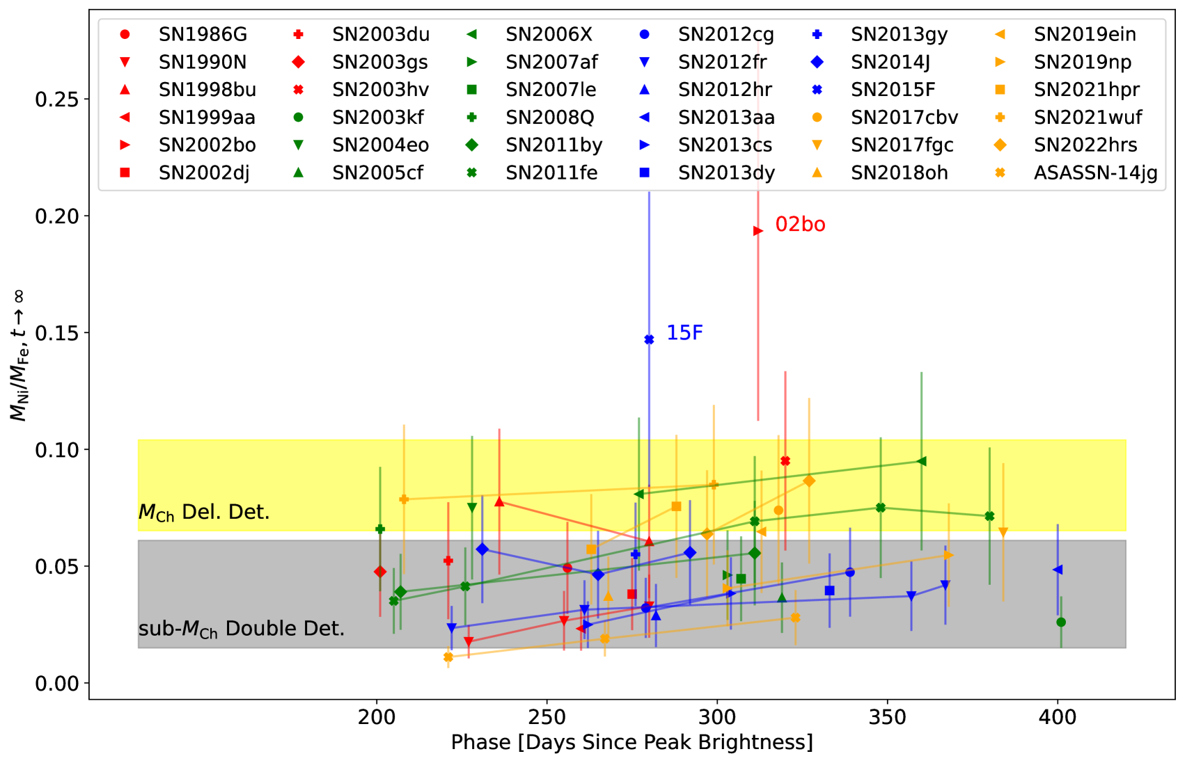
Figure 6: The inferred mass ratio of Ni and Fe as a function of phase after maximum light for SNe Ia collected in this work. The large error bars are mainly due to the $\sim 40$% relative uncertainty of the estimate of Maguire et al. (2018) that we adopt. Following Flörs et al. (2020), the Ni/Fe ratio range predicted for the DDT models (Seitenzahl et al., 2013) is shown by the yellow band and that of the sub-$M_{\rm Ch}$ models (Shen et al., 2018) is represented by the grey band. Both the Ni/Fe ratios measured from the observed spectra and those predicted by the explosion models are scaled to $t\rightarrow\infty$ by assuming a rise time of $\sim 18$ d (Ganeshalingam et al., 2011).

4.3 Connection between Ni/Fe Ratios and Si Velocities

To find some potential correlations between Ni/Fe ratios and early-time observed properties, we use the $t\approx 300$ days spectra whenever possible, since the parameters that we adopt to infer the Ni/Fe ratio come from the W7 model at $t\approx 330$ days (Fransson & Jerkstrand, 2015). Note that $t\approx+300$ days is the median of the phase range ($\sim+200$–400 days) of our sample.

The distribution of the inferred Ni/Fe mass ratios and the Si II $\lambda$6355 velocities measured around the time of maximum light is shown in Fig. 7, where one can see that the $M_{\rm Ni}/M_{\rm Fe}$ ratio tends to increase with Si II velocity. Moreover, the subsamples with redshifted or blueshifted nebular velocities seem to follow distinct $M_{\rm Ni}/M_{\rm Fe}$–$v_{\rm Si~{}II}$ relations. To test the robustness of the above correlation, we further use the scipy package’s stats.pearsonr function to calculate the Pearson coefficient. The correlations are found to be prominent for both the blueshifted and redshifted subsamples when not considering the error bars, with the $r$-values being black0.53 and 0.61, and the $p$-values being black0.03 and 0.03, respectively. blackWhen combining the whole sample, the correlation seems to be less prominent, with the $r$-value being only 0.32, and the $p$-value being 0.07. For the case including error bars, we assume a Gaussian distribution for the quoted uncertainties and repeat the calculation 20,001 times with a Monte Carlo method. If selecting the middle number of the Monte Carlo results, the significance of the correlations becomes more ambiguous, with the $r$-values being black0.32 and 0.38, and the $p$-values being black0.21 and 0.19, for the blueshifted and redshifted subsamples, respectively. Nevertheless, the connection is in agreement with some previous work and will be further discussed in Section 5.2.

From the histograms shown in Fig. 7, we can see that all SNe Ia with blueshifted Ni/Fe velocities in the nebular phase have Si velocities $<12,000$ km s^-1 except for SN 2021wuf, while those with redshifted nebular velocities have Si velocities ranging from 10,000 km s^-1 to black$\sim 17,000$ km s^-1. The range of the Ni/Fe ratio is similar for these two subgroups. We also notice that when the Si velocity is near 10,000 km s^-1, the two groups with blueshifted and redshifted Ni/Fe velocities tend to mix.

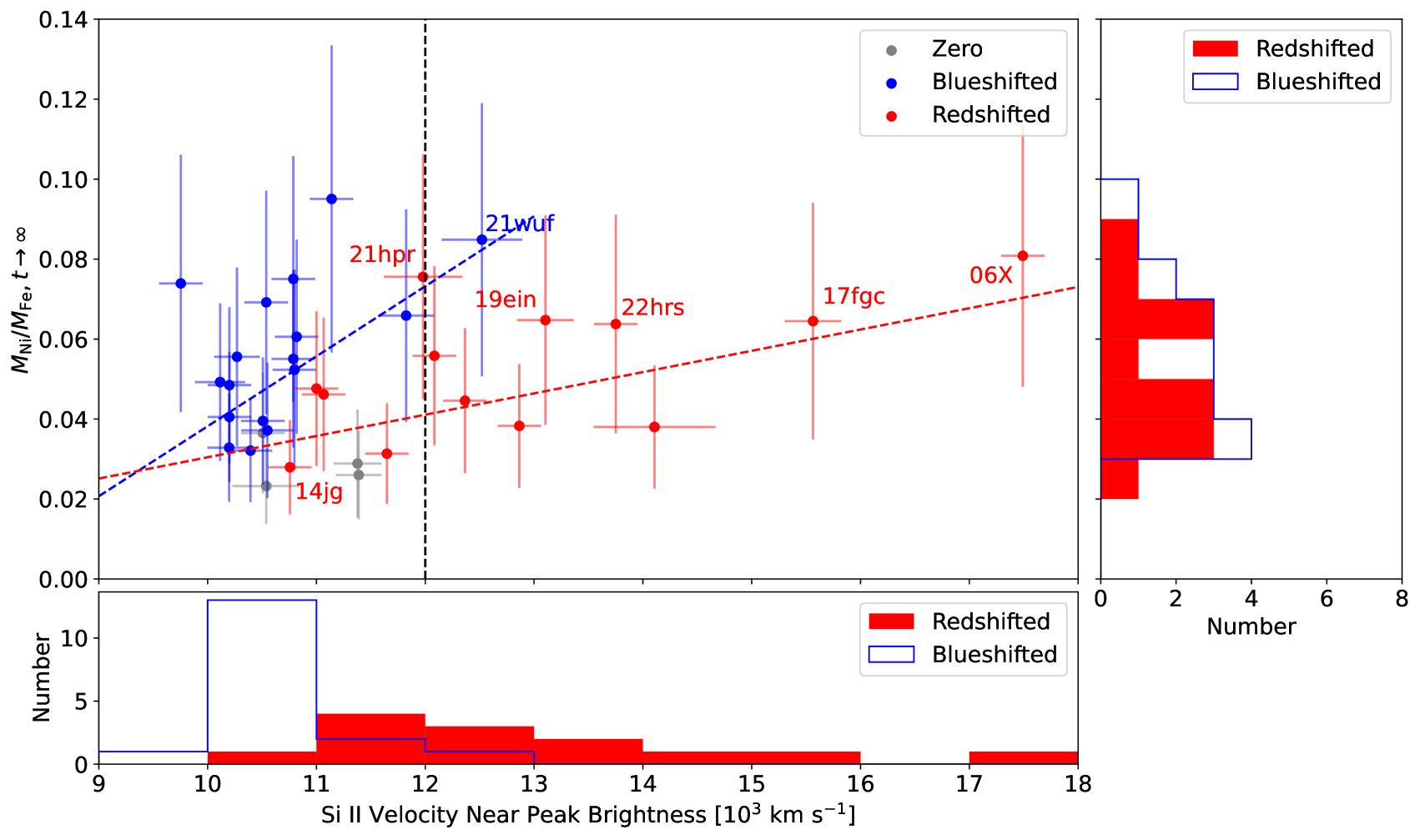
Figure 7: Inferred Ni/Fe mass ratio versus the Si II 6355 Å velocity measured around the time of maximum light. SNe Ia that have redshifted or blueshifted nebular velocities are shown by red and blue circles, respectively, while those with nebular velocities close to zero are represented by grey dots. The red and blue dashed lines represent the best linear fits to the data points with redshifted and blueshifted nebular velocities, respectively. The horizontal and vertical histograms represent the distributions of Si velocities and Ni/Fe ratios.

4.4 Connection between the Ni/Fe Ratio and $\Delta m_{15}(B)$

Fig. 8 shows the relation between the Ni/Fe mass ratio and $\Delta m_{15}(B)$. Note that SNe Ia with blueshifted and redshifted nebular velocities tend to mix in the plot, in contrast to the distinct distribution seen in Fig. 7. The Ni/Fe mass ratio seems to increase with $\Delta m_{15}(B)$, with fast decliners having larger Ni/Fe mass ratio. However, this correlation reverses for SNe Ia with larger post-peak decline rates — that is, the SNe Ia with black$\Delta m_{15}(B)>1.7$ mag have small Ni/Fe mass blackratio. blackThis discrepancy is likely related to the intrinsic difference existing between the SN 1991bg-like (SN 1986G and SN 2003gs in Fig. 8) and other SNe Ia. In addition, we caution about the low Ni/Fe ratio inferred for the overluminous SN 1991T-like SN 1999aa, which favours a sub-$M_{\rm Ch}$ explosion. Note that the sub-$M_{\rm Ch}$ detonation model of Shen et al. (2018) of a relatively massive WD (1.1 M_⊙) shows lower luminosity than the overluminous SN Ia; thus, it seems to be hard for the sub-$M_{\rm Ch}$ model to produce the high luminosity.

We calculate the Pearson’s $r$-values for all of the sample shown in Fig. 8, except SN 1986G and SN 2003gs. We obtain an $r$-value of black0.68 and a $p$-value of black$2.18\times 10^{-5}$ without considering the error bars, and an $r$-value of black0.43 and a $p$-value of black0.01 when including the error bars with the Monte Carlo method adopted in Section 4.3. These results strongly suggest that the inferred Ni/Fe mass ratio has a positive correlation with $\Delta m_{15}(B)$.

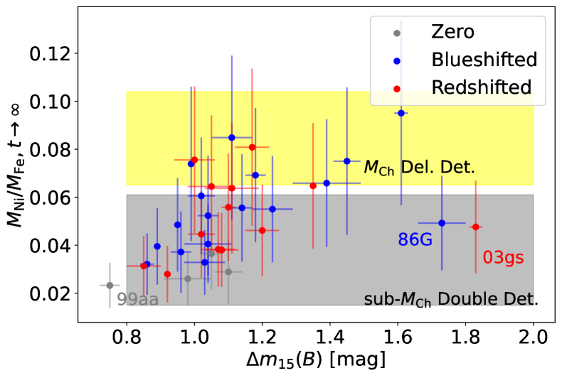
Figure 8: Inferred mass ratio of Ni and Fe versus the post-peak decline rate $\Delta m_{15}(B)$. The symbols are the same as in Fig. 7. Yellow and grey regions represent the explosion models as indicated in Fig. 6.

5 Discussion

In this paper, we applied multicomponent Gaussian fits to the spectral features near 7300 Å for 36 SNe Ia. Nebular velocities and Ni/Fe mass ratios are inferred from the velocity shifts and flux ratios, respectively. In this section, we further discuss the evolution of the inferred Ni/Fe ratio, and we explore possible connections between inferred late-time parameters and early-time parameters and their implications for explosion mechanisms.

5.1 blackEvolution of the 7300 Å region

For the well-observed object SN 2011fe, we notice that the inferred Ni/Fe ratio shows temporal evolution, moving from the regions favouring the sub-$M_{\rm Ch}$ double-detonation model to that favouring the $M_{\rm Ch}$ delayed detonation model. blackThe increasing trend is also found for other events having at least three spectra except for SN 2014J. Considering the uncertainties using a Monte Carlo method, the mean Pearson $r$-value derived for SNe 1990N, 2011fe, 2012fr, and ASASSN-14jg is $0.73\pm 0.11$. Note that the variation inferred for the Ni/Fe ratio with phase only reflects the evolution of the flux ratio of [Ni II] 7378 Å and [Fe II] 7155 Å, since we use the same temperature and departure coefficients to infer the Ni/Fe ratio in all phases as Maguire et al. (2018) did. It should be noted that the errors associated with the Ni/Fe ratio shown in Fig. 6 are dominated by uncertainties in temperature and departure coefficients ratio, which might be overestimated when analysing the evolution for the same object. This is due to the fact that the temperature usually decreases with time while the departure coefficients increase with time for the same object, and the net evolution effect of these two parameters on the inferred Ni/Fe ratio is thus limited.

blackNote that we use the same temperature and ratio of departure coefficients to infer the Ni/Fe ratio, hence the evolution of the Ni/Fe ratio is due to the evolution of the flux ratio of [Ni II] 7378 Å and [Fe II] 7155 Å. This evolution is clearly indicated in Fig. 2, where the [Ni II] 7378 Å feature tends to become increasingly prominent compared with the [Fe II] 7155 Å feature, which might be due to the suppression of the [Ni II] lines as a result of higher ionisation of nickel in the inner ejecta (Blondin et al., 2022). As the inner ejecta cool gradually, the flux ratio of [Ni II] to [Ni III] increases with time, leading to the increase of the inferred Ni/Fe ratio. blackIn fact, we also notice that the scaled flux of the 7900 Å region decreases with time and this region could have a contribution from [Ni III] 7890 Å. Thus, the spectral evolution might indicate the recombination of [Ni III], since the flux-density ratio of [Ni II] 7378 Å and the 7900 Å region increases with time. Moreover, the high-quality spectra of SN 2011fe show that there exists a weak feature in the 7900 Å region, which nearly disappears at later phases.

blackAnother possible reason for the increase of the flux ratio of [Ni II] 7378 Å and [Fe II] 7155 Å is that the [Fe II] 7155 Å feature is contributed by the bump that gets weaker with time. Fig. 2 also shows the evolution of the spectra subtracting the pseudocontinuums defined by point $A^{\prime}$, where the bump (likely related to some additional features that only contribute at early times) is subtracted. In this case, the trend that the flux ratio of [Ni II] 7378 Å and [Fe II] 7155 Å increase with time is still visible. But if the bump contributes little to the [Ni II] 7378 Å feature, the strength of the [Ni II] 7378 Å feature will be underestimated when subtracting the pseudocontinuums defined by point $A^{\prime}$. A more careful fitting that includes some new emission lines related to the bump is needed to confirm the evolution, which is more complicated and beyond the scope of this paper.

Flörs et al. (2020) used an NLTE level population model to fit the full late-time spectra for their SN Ia sample and found no evident evolution for Ni/Fe ratios for a given object. In Fig. 9, we compare our inferred Ni/Fe ratios with those predicted by Flörs et al. (2020) for the same spectra. We also show the comparison of the Ni/Fe ratios between case $A$ and case $A^{\prime}$. blackThe results from Flörs et al. (2020) and ours are in good agreement at phases $t\lesssim+300$ days. When approaching $t\gtrsim+300$ days, our fits tend to give systematically larger Ni/Fe ratios. A possible interpretation is that the evolution of the Ni/Fe ratio disappears when more accurate temperatures, departure coefficients, and flux ratios are obtained through the NLTE calculations and full spectral fitting. But we notice that the 7900 Å region is not fit well by Flörs et al. (2020), which might also lead to the different results. For case $A$ and case $A^{\prime}$, the Ni/Fe mass ratios inferred from the spectra taken at $t>+300$ days are more similar, since the small bump at 6800–7000 Å that leads to the different pseudocontinua becomes weak at such phases.

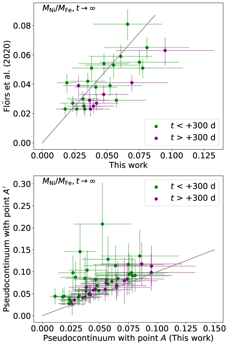
Figure 9: Comparisons of the Ni/Fe ratios given by different methods. The top panel compares our fits with those from the NLTE model of Flörs et al. (2020) for the same spectra. The labeled objects are those whose Ni/Fe ratios deviate by more than 1$\sigma$. The bottom panel compares the fits using point $A$, which defines a similar pseudocontinuum to that of Maguire et al. (2018), with the fits using point $A^{\prime}$, which is adopted in this work. The Ni/Fe ratios inferred from the spectra taken at $t<+300$ days are shown with green dots while those taken at $t>+300$ days are shown with purple dots.

It should be noted that the evolution of the inferred Ni/Fe ratio makes the distinction between $M_{\rm Ch}$ models and sub-$M_{\rm Ch}$ models difficult. If the evolution is caused by suppression of [Ni II], more-accurate estimates of the Ni/Fe ratio could be inferred from very late-phase spectra, at $t\gtrsim+350$ days when the minor emission on the left side of the $\sim 7300$ Å feature disappears in the spectra. Considering such an evolutionary trend, a relatively lower Ni/Fe ratio inferred from earlier nebular-phase spectra (i.e., at $t\approx 250$ days) should be used carefully to confine the explosion models. For our sample, black7 and 12 out of 19 SNe Ia are found to be more in favour of the $M_{\rm Ch}$ and sub-$M_{\rm Ch}$ models, respectively, if restricting the SN Ia sample to those with at least one spectrum at $t>+300$ days. The relative fractions (i.e., about black$37\%$ for $M_{\rm Ch}$ and black$63\%$ for sub-$M_{\rm Ch}$) are consistent with the results derived for the whole sample. However, the proportion favouring an origin in sub-$M_{\rm Ch}$ explosions still could be overestimated because the inferred low Ni/Fe ratio might be affected by spectral evolution.

5.2 Implications for the Variation of Si Velocities

Maeda et al. (2010a) found that Si velocity gradients were correlated with nebular velocities, and they proposed an asymmetric and off-centre explosion toy model to interpret this correlation as a geometric effect. In particular, one will find low-velocity-gradient (LVG) SNe Ia when viewing from the direction of off-centre ignition and high-velocity-gradient (HVG) SNe Ia from the opposite direction. A similar correlation can be found between Si velocities at maximum light and nebular velocities (Silverman et al., 2013). Fig. 7 shows that almost all HV SNe Ia display a redshifted nebular velocity, in agreement with Silverman et al. (2013). Note that the HV subclass is not bound exactly to the HVG subclass; for example, SN 2021wuf can be put into the HV group while its Si velocity gradient is relatively low (LVG). Nevertheless, to do the analysis we use the Si velocity around the time of maximum light instead of the Si velocity gradient, since the former parameter is more convenient to measure.

As indicated in Fig. 7, the two branches of SNe Ia characterised by redshifted or blueshifted nebular velocities show distinct distributions in the Ni/Fe ratio and Si II velocity plane, especially at the larger velocity end where no blueshifted SNe Ia are found except for SN 2021wuf. The histogram distribution of the Ni/Fe ratio and Si II velocity indicates that the separation between redshifted and blueshifted objects is caused mainly by Si velocity instead of the Ni/Fe ratio.

To examine whether the blueshifted and redshifted objects at lower velocities also come from different groups, we applied a two-dimensional K-S test (Fasano & Franceschini, 1987) and derived the $p$-value as black0.05. Such a small $p$-value suggests that the blueshifted and redshifted branches still show a significant difference. Nevertheless, we caution that this result may suffer from small-number statistics (especially for redshifted NV objects), and a larger sample is needed for further analysis. blackNote that the correlation between the Ni/Fe ratio and Si velocity is weak for the whole sample, with a Pearson $r$-value being 0.31 even when not considering the uncertainties. Thus, we focus on the subsamples with redshifted or blueshifted nebular velocities in the following analysis in this subsection.

In the study by Maeda et al. (2010a), the LVG SNe Ia displaying redshifted nebular velocities were not regarded as exceptions, and they suggested that SNe Ia of the LVG and HVG subclasses do not have intrinsic differences as long as the redshifted nebular velocity is not too large (i.e., $\lesssim 1000$ km s^-1). However, the blackpossible LVG SN Ia ASASSN-14jg (Graham et al., 2017), with Si velocity black$\sim 10,760$ km s^-1 at +6 days, has an unusually large redshifted nebular velocity black($\sim 1600$ km s^-1) relative to the expected upper limit of $\sim 1000$ km s^-1. This suggests that ASASSN-14jg could still be observed in the NV subclass when viewing from the opposite direction of off-centre ignition owing to its overall low Si velocity. Moreover, among the redshifted objects, black$\sim 40$% are found to have normal Si velocity (i.e., $\lesssim 12,000$ km s^-1), which means that it is not rare that NV SNe Ia display redshifted nebular velocities. Thus, other factors are needed to interpret the variation of Si velocities.

On the other hand, Wang et al. (2013) found that HV SNe Ia tend to occur in inner regions of their host galaxies, arguing that the diversity of Si velocities in SNe Ia cannot be completely attributed to geometric effects and HV SNe Ia may be related to metal-rich stellar populations (Pan et al., 2015a; Pan, 2020). This is consistent with the recent result that HV SNe Ia tend to have abundant circumstellar dust (Wang et al., 2019). The analysis of late-time spectral features presented in this paper also supports that HV SNe Ia may have metal-rich progenitors. Timmes et al. (2003) explored how the ratio of stable-to-radioactive nucleosynthetic products increases with the metallicity of SN progenitors. A higher ratio of stable-to-radioactive nucleosynthetic products means a higher late-time Ni/Fe ratio, since all of the radioactive ⁵⁶Ni would decay to ⁵⁶Co and finally ⁵⁶Fe. This has also been discussed by Graham et al. (2022). If we only focus on the SNe Ia that have redshifted or blueshifted nebular velocities, the Ni/Fe ratio tends to increase with Si velocity, so the Si velocity has a positive correlation with metallicity. This correlation is also in agreement with the simulated result that the blueshift of Si II absorption increases with the metallicity of the C+O layer of SN Ia progenitors (Lentz et al., 2000). Thus, the low Si velocity of ASASSN-14jg may be due to its low Ni/Fe ratio (low metallicity). However, we caution that whether the variation of metallicity can completely account for the observed variation of Si velocity is not clear, and more-detailed explosion simulations are needed in future work.

5.3 Sub-$M_{\rm Ch}$ Models Prefer Smaller $\Delta m_{15}(B)$?

As shown in Fig. 8, a positive correlation between the Ni/Fe ratio and $\Delta m_{15}(B)$ seems to exist for SNe Ia with black$\Delta m_{15}<1.7$ mag. A higher Ni/Fe ratio means a higher ratio of stable-to-radioactive nucleosynthetic products and hence a lower mass of synthetic radioactive ⁵⁶Ni. The mass of radioactive ⁵⁶Ni is a dominant parameter describing the explosion energy of SNe Ia, with larger ⁵⁶Ni corresponding to a more energetic explosion and hence smaller $\Delta m_{15}(B)$. Thus, given a similar total mass of ejecta, a higher ratio of stable-to-radioactive nucleosynthetic products would naturally result in a fainter SN Ia with larger $\Delta m_{15}(B)$.

However, the positive correlation between the Ni/Fe ratio and $\Delta m_{15}(B)$ also implies that the sub-$M_{\rm Ch}$ models would tend to produce more-luminous SNe Ia than the $M_{\rm Ch}$ models, contradicting the previous understanding of explosion models. Considering the [Ni II] suppression that we have discussed in Section 5.1, an alternative interpretation is that SNe Ia with smaller $\Delta m_{15}(B)$ might have more radioactive materials, which would ionise more nickel to Ni III at late phases. blackThis interpretation is supported by the finding of Blondin et al. (2022) that the strong [Ni II] lines predicted by their $M_{\rm Ch}$ models can be completely suppressed when ⁵⁶Ni is sufficiently mixed with the stable iron-group elements. Thus, the Ni/Fe ratio inferred from our methods would be underestimated for more-luminous SNe Ia. In other words, the positive correlation between the inferred Ni/Fe ratio and $\Delta m_{15}(B)$ is caused by different degrees of suppression of [Ni II] features.

6 Conclusions

We have performed multicomponent Gaussian fits to the 7300 Å emission features (due to [Fe II] and [Ni II]) in the nebular spectra of 36 SNe Ia. This has allowed us to measure the velocity shifts and flux ratios of [Ni II] and [Fe II] features in this region, which can be used to infer nebular velocities and the late-time Ni/Fe ratio, respectively. The nebular velocity might be connected to the geometry of the explosion, while the Ni/Fe ratio can be used to distinguish sub-$M_{\rm Ch}$ and $M_{\rm Ch}$ models. Connecting these inferred late-time parameters with the early-time observations (Si II $\lambda$6355 velocity at maximum light and $\Delta m_{15}(B)$), we find some interesting correlations. Our main results are as follows.

(i) The majority (about black67%) of SNe Ia in this work favour sub-$M_{\rm Ch}$ models. However, this fraction could be overestimated owing to a potentially increasing trend of the inferred Ni/Fe ratio with SN age. Moreover, the increasing trend can be interpreted as the suppression of [Ni II] lines as a result of higher ionisation of nickel in the inner ejecta.

(ii) blackAlthough the whole sample do not show a prominent correlation between the inferred Ni/Fe ratio and Si velocity, a positive correlation tends to exist for subsamples with redshifted or blueshifted nebular velocities. This indicates that the progenitor metallicity should be at least partially responsible for the variation of Si velocity observed in SNe Ia.

(iii) The Ni/Fe ratio has a positive correlation with $\Delta m_{15}(B)$, except for the SN 1991bg-like SNe Ia. This correlation seems to suggest that sub-$M_{\rm Ch}$ explosions tend to produce more-luminous SNe Ia than $M_{\rm Ch}$ explosions, which violates common sense. However, this correlation could be caused by serious suppression of [Ni II] (ionised to [Ni III]) for luminous SNe Ia with smaller $\Delta m_{15}(B)$.

Late-time spectra reveal the inner region of SNe Ia and are important in studying the explosion properties. Connections between the inner region and the outer ejecta also have many implications for the study of explosion mechanisms. In future work, more high-quality late-time spectra are needed to confirm these connections and explore new correlations. Additional well-observed SNe Ia at late phases are also needed to study the evolution of late-time spectra and give more-accurate estimates of the Ni/Fe ratio to confine explosion models.

Data Availability

The data underlying this article are available in the article. Information on the spectra collected by our own project is presented in Table 1. Some basic information about the SNe Ia in this work is presented in Table 2. The fits for all spectra in this work are shown in Fig. 10, and the corresponding parameters are presented in Table 3.

Appendix A Overview of SNe Ia and Fitting Results

Table 2: SNe Ia light curve, spectral, and host-galaxy information.

Name	Typea	Host galaxy	Redshift	$A_{V}$b	$\Delta m_{15}(B)$	blackSi vel., Phase	Date of max.c	Ref.d	Ref.e	Ref.
				[mag]	[mag]	[1000 $\rm km\ s^{-1}$, d]	UTC	Spec.	LC	$A_{V}$
SN 2019ein	pec	NGC 5353	0.007755	0.033	1.35$\pm$0.01	13.10$\pm$0.26, +0	20190516	1	2	3
SN 2019np	norm	NGC 3254	0.00452	0.054	1.04$\pm$0.07	10.20$\pm$0.20, +0	20190127	4	4	3
SN 2021hpr	norm	NGC 3147	0.009346	0.065	1.0$\pm$0.06	11.98$\pm$0.36, +1	20210418	5	5	3
SN 2021wuf	norm	NGC 6500/NGC 6501	0.01	0.241	1.11$\pm$0.06	12.52$\pm$0.37, +1	20210905	6	6	3
SN 2022hrs	norm	NGC 4647	0.0047	0.744	1.11$\pm$0.08	13.75$\pm$0.20, +0	20220429	7	7	7,3
SN 1986G	91bg	NGC 5128	0.001825	2.79	1.73$\pm$0.07	10.11$\pm$0.23, +0	19860511	8	9,10	9
SN 1990N	norm	NGC 4639	0.003369	0.069	1.03$\pm$0.06	10.20$\pm$0.20, +2	19900710	11	12	3
SN 1998bu	norm	NGC 3368	0.002992	1.054	1.02$\pm$0.04	10.82$\pm$0.20, -1	19980519	13	14	14
SN 1999aa	91T	NGC 2595	0.014907	0.106	0.75$\pm$0.03	10.54$\pm$0.31, -1	19990222	15	16	3
SN 2002bo	norm	NGC 3190	0.0043	1.333	1.13$\pm$0.05	13.41$\pm$0.31, +0	20020323	17	17	17
SN 2002dj	norm	NGC 5018	0.009393	0.254	1.08$\pm$0.05	14.11$\pm$0.56, -3	20020624	18	18	3
SN 2003du	norm	NGC 9391	0.006408	0.027	1.04$\pm$0.03	10.80$\pm$0.20, +0	20030506	19	20	3
SN 2003gs	91bg	NGC 936	0.00477	0.094	1.83$\pm$0.02	11.00$\pm$0.20, +2	20030728	21	22	3
SN 2003hv	norm	NGC 1201	0.005624	0.041	1.61$\pm$0.02	11.14$\pm$0.20, +1	20030909	23	23	3
SN 2003kf	norm	MCG -02-16-002	0.0074	0.833	0.98$\pm$0.07	11.39$\pm$0.21, -3	20031207	24	25	3
SN 2004eo	norm	NGC 6928	0.015718	0.288	1.45$\pm$0.04	10.79$\pm$0.20, -3	20040930	26	26	3
SN 2005cf	norm	MCG -01-39-003	0.006461	0.261	1.05$\pm$0.03	10.51$\pm$0.20, +0	20050612	27	28	3
SN 2006X	norm	NGC 4321	0.005294	2.172	1.17$\pm$0.05	17.49$\pm$0.20, +0	20060219	29	29	29,3
SN 2007af	norm	NGC 5584	0.005464	0.104	1.2$\pm$0.05	11.07$\pm$0.20, +0	20070314	24	30,25	3
SN 2007le	norm	NGC 7721	0.006721	0.71	1.02$\pm$0.04	12.36$\pm$0.20, +3	20071025	31	32,33	32,3
SN 2008Q	norm	NGC 524	0.0081	0.221	1.39$\pm$0.1	11.82$\pm$0.26, +0	20080209	24	34	3
SN 2011by	norm	NGC 3972	0.002843	0.037	1.14$\pm$0.03	10.27$\pm$0.21, +1	20110509	33	33	3
SN 2011fe	norm	M 101	0.000804	0.024	1.18$\pm$0.03	10.54$\pm$0.20, +0	20110910	35	36	3
SN 2012cg	91T	NGC 4424	0.001458	0.62	0.86$\pm$0.02	10.39$\pm$0.20, +3	20120603	37	37	38,3
SN 2012fr	norm	NGC 1365	0.004	0.054	0.85$\pm$0.05	11.65$\pm$0.20, +0	20121112	39	40	3
SN 2012hr	norm	ESO 121-G026	0.008	0.121	1.1$\pm$0.04	11.38$\pm$0.22, +5	20121228	41	42	3
SN 2013aa	norm	NGC 5643	0.003999	0.453	0.95$\pm$0.01	10.20$\pm$0.20, +0	20130220	41	43	3
SN 2013cs	norm	ESO 576-G017	0.00924	0.248	1.07$\pm$0.05	12.86$\pm$0.20, +1	20130525	44	45	3
SN 2013dy	norm	NGC 7250	0.00389	0.409	0.89$\pm$0.01	10.51$\pm$0.20, +1	20130728	46	46	3
SN 2013gy	norm	NGC 1418	0.014023	0.154	1.23$\pm$0.06	10.79$\pm$0.20, -1	20131222	47	47	3
SN 2014J	norm	NGC 3034	0.000677	2.421	1.1$\pm$0.02	12.08$\pm$0.20, +0	20140201	48	49	50,3
SN 2015F	norm	NGC 2442	0.0049	0.542	1.35$\pm$0.03	10.44$\pm$0.23, -3	20150325	51	52	3
SN 2017cbv	norm	NGC 5643	0.003999	0.45	0.99$\pm$0.01	9.75$\pm$0.20, -1	20170328	53	54	3
SN 2017fgc	norm	NGC 0474	0.008	0.091	1.05$\pm$0.07	15.56$\pm$0.26, +1	20170725	55	56	3
SN 2018oh	norm	UGC 04780	0.012	0.12	0.96$\pm$0.03	10.55$\pm$0.24, +0	20180213	57	57	3
ASASSN-14jg	norm	PGC 128348	0.0148	0.04	0.92$\pm$0.01	10.76$\pm$0.20, +6	20141031	44	41	3

blackReference: (1) Pellegrino et al. (2020); (2) Xi et al. (2022); (3) Schlafly & Finkbeiner (2011); (4) Sai et al. (2022); (5) Iskandar et al. (in prep.); (6) Zeng et al. (in prep.); (7) Liu et al. (in prep.); (8) Cristiani et al. (1992); (9) Phillips et al. (1987); (10) Phillips et al. (1999); (11) Mazzali et al. (1993); (12) Lira et al. (1998); (13) Matheson et al. (2008); (14) Jha et al. (1999); (15) Silverman et al. (2012a); (16) Krisciunas et al. (2000); (17) Benetti et al. (2004); (18) Pignata et al. (2008); (19) Gerardy (2005); (20) Anupama et al. (2005); (21) Evans et al. (2003); (22) Krisciunas et al. (2009); (23) Leloudas et al. (2009); (24) Blondin et al. (2012); (25) Hicken et al. (2009); (26) Pastorello et al. (2007); (27) Garavini et al. (2007); (28) Wang et al. (2009a); (29) Wang et al. (2008); (30) Simon et al. (2007); (31) Folatelli et al. (2013); (32) Simon et al. (2009); (33) Silverman et al. (2013); (34) Milne et al. (2010); (35) Pereira et al. (2013); (36) Zhang et al. (2016); (37) Marion et al. (2016); (38) Silverman et al. (2012b); (39) Childress et al. (2013); (40) Zhang et al. (2014); (41) Graham et al. (2017); (42) Brown et al. (2014); (43) Burns et al. (2020); (44) Childress et al. (2016); (45) Walker et al. (2015); (46) Pan et al. (2015b); (47) Holmbo et al. (2019); (48) Srivastav et al. (2016); (49) Li et al. (2019b); (50) Foley et al. (2014); (51) Foley et al. (2016); (52) Cartier et al. (2017); (53) Hosseinzadeh et al. (2017); (54) Wang et al. (2020); (55) Stahl et al. (2020); (56) Zeng et al. (2021); (57) Li et al. (2019a). The sample from our own project are put at the top of the table and separated from the public sample by a line.

^aThe type is estimated with SNID (Blondin & Tonry, 2007) using the spectrum around the maximum light except for SN 2003gs, SN 2013aa, and SN 2019ein, whose classifications are taken from Krisciunas et al. (2009), Parker et al. (2013), and Burke et al. (2019), respectively.

^bWe assume host $R_{V}=3.1$ except for SN 2006X, SN 2007le, and SN 2014J, whose host $R_{V}$ values are 1.48, 2.56, and 1.6, respectively.

^cThe date of $B$-band maximum light used in this work.

^dSources for the spectra used to calculate Si II $\lambda$6355 velocities around the time of $B$-band maximum and identify the type. The Si II $\lambda$6355 velocities of SN 2003gs and SN 2013aa are taken from Evans et al. (2003) and Graham et al. (2017), respectively.

^eReferences for the date of $B$-band maximum and $\Delta m_{15}(B)$. For SN 2003kf, SN 2012hr, and SN 2013cs, these two parameters are measured in this work with SALT2 using the light curves from the references.

Table 3: Multicomponent Gaussian-fit parameters of nebular-phase emission lines, and implications.

Name	Phase	[Fe II] Vel.	[Ni II] Vel.	[Fe II] FWHM	[Ni II] FWHM	Flux ratio	Nebular Vel.	$M_{\rm Ni}$/$M_{\rm Fe}$	Ref.
	[days]	[km s-1]	[km s-1]	[km s-1]	[km s-1]	$\lambda$7155/$\lambda$7378	[km s-1]	$t\rightarrow\infty$	Spec.
SN 2019ein	+313	-11$\pm$623	2436$\pm$326	12531$\pm$434	4368$\pm$379	0.370$\pm$0.023	2436$\pm$326	0.065$\pm$0.026	1
SN 2019np	+303	-1700$\pm$227	-3258$\pm$412	6980$\pm$80	5520$\pm$240	0.233$\pm$0.008	-1700$\pm$227	0.041$\pm$0.016	2
SN 2019np	+368	-1526$\pm$318	-3057$\pm$404	7128$\pm$331	5639$\pm$79	0.305$\pm$0.018	-1526$\pm$318	0.055$\pm$0.022	2
SN 2021hpr	+263	790$\pm$249	125$\pm$325	7453$\pm$626	5366$\pm$236	0.338$\pm$0.036	790$\pm$249	0.057$\pm$0.024	3
SN 2021hpr	+288	623$\pm$231	676$\pm$295	8363$\pm$222	5998$\pm$82	0.438$\pm$0.028	623$\pm$231	0.076$\pm$0.031	3
SN 2021wuf	+208	-3226$\pm$351	-2776$\pm$242	7691$\pm$162	4597$\pm$207	0.494$\pm$0.038	-2776$\pm$242	0.079$\pm$0.032	4
SN 2021wuf	+299	-3040$\pm$467	-2503$\pm$362	9977$\pm$144	4880$\pm$266	0.488$\pm$0.022	-2503$\pm$362	0.085$\pm$0.034	4
SN 2022hrs	+297	628$\pm$554	777$\pm$403	9064$\pm$213	6097$\pm$359	0.367$\pm$0.057	628$\pm$554	0.064$\pm$0.027	5
SN 2022hrs	+327	890$\pm$498	739$\pm$657	8212$\pm$515	6510$\pm$357	0.491$\pm$0.044	890$\pm$498	0.087$\pm$0.035	5
SN 1986Ga	+256	-965$\pm$237	-965$\pm$237	8109$\pm$163	3569$\pm$393	0.293$\pm$0.005	-965$\pm$237	0.049$\pm$0.020	6
SN 1990N	+227	-1696$\pm$236	-3606$\pm$323	8875$\pm$192	6472$\pm$103	0.108$\pm$0.007	-1696$\pm$236	0.018$\pm$0.007	7
SN 1990N	+255	-1354$\pm$274	-1827$\pm$569	9268$\pm$272	6655$\pm$806	0.158$\pm$0.042	-1354$\pm$274	0.027$\pm$0.013	7
SN 1990N	+280	-1315$\pm$229	-1968$\pm$418	9017$\pm$114	8165$\pm$358	0.191$\pm$0.018	-1315$\pm$229	0.033$\pm$0.014	7
SN 1998bu	+236	-1322$\pm$227	-1604$\pm$272	8198$\pm$68	5533$\pm$319	0.471$\pm$0.020	-1322$\pm$227	0.078$\pm$0.031	8
SN 1998bu	+280	-1429$\pm$265	-1686$\pm$289	8393$\pm$437	4824$\pm$303	0.353$\pm$0.009	-1429$\pm$265	0.061$\pm$0.024	8
SN 1999aa	+260	114$\pm$263	-209$\pm$277	8030$\pm$100	3392$\pm$211	0.138$\pm$0.009	114$\pm$263	0.023$\pm$0.009	8
SN 2002bo	+312	1251$\pm$278	1859$\pm$324	7505$\pm$579	8452$\pm$668	1.105$\pm$0.143	1251$\pm$278	0.194$\pm$0.081	9
SN 2002dj	+275	1224$\pm$276	2202$\pm$334	9535$\pm$210	5445$\pm$208	0.222$\pm$0.015	1224$\pm$276	0.038$\pm$0.015	10
SN 2003du	+221	-2001$\pm$292	-3024$\pm$741	8112$\pm$355	8075$\pm$803	0.323$\pm$0.085	-2001$\pm$292	0.052$\pm$0.025	11
SN 2003gsa	+201	807$\pm$258	807$\pm$258	9687$\pm$212	4932$\pm$87	0.303$\pm$0.021	807$\pm$258	0.048$\pm$0.019	8
SN 2003hv	+320	-2575$\pm$218	-3688$\pm$257	8525$\pm$225	4984$\pm$107	0.541$\pm$0.030	-3688$\pm$257	0.095$\pm$0.038	12
SN 2003kf	+401	302$\pm$396	115$\pm$728	10651$\pm$212	4944$\pm$1585	0.144$\pm$0.021	302$\pm$396	0.026$\pm$0.011	9
SN 2004eo	+228	-994$\pm$249	-2266$\pm$352	8329$\pm$149	8556$\pm$325	0.459$\pm$0.040	-994$\pm$249	0.075$\pm$0.031	13
SN 2005cf	+319	67$\pm$237	-84$\pm$1647	8574$\pm$1106	6790$\pm$461	0.208$\pm$0.021	67$\pm$237	0.036$\pm$0.015	14
SN 2006X	+277	2298$\pm$277	2248$\pm$237	8052$\pm$114	5434$\pm$117	0.472$\pm$0.031	2298$\pm$277	0.081$\pm$0.033	15
SN 2006X	+360	2731$\pm$235	2488$\pm$244	9182$\pm$212	5272$\pm$72	0.531$\pm$0.024	2731$\pm$235	0.095$\pm$0.038	8
SN 2007af	+303	421$\pm$226	367$\pm$349	7744$\pm$367	5775$\pm$223	0.265$\pm$0.029	421$\pm$226	0.046$\pm$0.019	9
SN 2007le	+307	1497$\pm$246	1614$\pm$293	8809$\pm$287	5238$\pm$77	0.255$\pm$0.019	1497$\pm$246	0.045$\pm$0.018	8
SN 2008Q	+201	-2239$\pm$318	-1485$\pm$228	11131$\pm$225	4765$\pm$29	0.419$\pm$0.024	-1485$\pm$228	0.066$\pm$0.027	8
SN 2011by	+207	-1536$\pm$277	-2845$\pm$488	7675$\pm$278	5547$\pm$435	0.246$\pm$0.029	-1536$\pm$277	0.039$\pm$0.016	16
SN 2011by	+311	-1066$\pm$212	-1716$\pm$243	7970$\pm$155	5080$\pm$40	0.318$\pm$0.013	-1066$\pm$212	0.056$\pm$0.022	16
SN 2011fe	+205	-1143$\pm$210	-2217$\pm$241	8423$\pm$78	5606$\pm$56	0.222$\pm$0.007	-1143$\pm$210	0.035$\pm$0.014	17
SN 2011fe	+226	-1027$\pm$229	-2077$\pm$308	8148$\pm$128	5709$\pm$145	0.254$\pm$0.012	-1027$\pm$229	0.041$\pm$0.017	18
SN 2011fe	+311	-1068$\pm$251	-1077$\pm$332	8329$\pm$215	7072$\pm$224	0.395$\pm$0.022	-1068$\pm$251	0.069$\pm$0.028	18
SN 2011fe	+348	-638$\pm$251	-1297$\pm$284	8507$\pm$107	6922$\pm$126	0.422$\pm$0.014	-638$\pm$251	0.075$\pm$0.030	19
SN 2011fe	+380	-340$\pm$297	-1047$\pm$356	9051$\pm$291	6980$\pm$226	0.397$\pm$0.038	-340$\pm$297	0.071$\pm$0.029	18
SN 2012cg	+279	-1070$\pm$223	-1830$\pm$354	7813$\pm$164	5603$\pm$94	0.187$\pm$0.005	-1070$\pm$223	0.032$\pm$0.013	20
SN 2012cg	+339	-1111$\pm$234	-841$\pm$314	8716$\pm$101	7279$\pm$141	0.267$\pm$0.010	-1111$\pm$234	0.047$\pm$0.019	21
SN 2012fr	+222	2041$\pm$264	2926$\pm$397	8033$\pm$93	5650$\pm$155	0.145$\pm$0.007	2041$\pm$264	0.023$\pm$0.009	22
SN 2012fr	+261	2030$\pm$219	2305$\pm$793	7338$\pm$785	5583$\pm$308	0.185$\pm$0.007	2030$\pm$219	0.031$\pm$0.013	22
SN 2012fr	+357	2205$\pm$226	2633$\pm$226	8059$\pm$52	5393$\pm$55	0.208$\pm$0.006	2205$\pm$226	0.037$\pm$0.015	21
SN 2012fr	+367	2085$\pm$248	3303$\pm$235	8799$\pm$267	4567$\pm$40	0.234$\pm$0.014	2085$\pm$248	0.042$\pm$0.017	22
SN 2012hr	+282	133$\pm$241	72$\pm$641	8342$\pm$349	7553$\pm$863	0.168$\pm$0.041	133$\pm$241	0.029$\pm$0.014	23
SN 2013aa	+400	-691$\pm$229	-1072$\pm$260	8237$\pm$113	6666$\pm$171	0.268$\pm$0.012	-691$\pm$229	0.048$\pm$0.020	23
SN 2013cs	+262	1474$\pm$234	2622$\pm$246	9232$\pm$68	4838$\pm$74	0.147$\pm$0.003	1474$\pm$234	0.025$\pm$0.010	23
SN 2013cs	+304	1343$\pm$245	1452$\pm$327	8179$\pm$170	6069$\pm$140	0.220$\pm$0.012	1343$\pm$245	0.038$\pm$0.015	21
SN 2013dy	+333	-1161$\pm$222	-1478$\pm$273	7664$\pm$97	6722$\pm$220	0.224$\pm$0.010	-1161$\pm$222	0.040$\pm$0.016	24
SN 2013gy	+276	-367$\pm$213	-438$\pm$402	8200$\pm$186	7044$\pm$259	0.322$\pm$0.015	-367$\pm$213	0.055$\pm$0.022	23
SN 2014J	+231	336$\pm$213	673$\pm$252	8291$\pm$88	9370$\pm$229	0.349$\pm$0.019	336$\pm$213	0.057$\pm$0.023	22
SN 2014J	+265	465$\pm$213	354$\pm$280	8071$\pm$116	7682$\pm$175	0.273$\pm$0.016	465$\pm$213	0.046$\pm$0.019	18
SN 2014J	+292	581$\pm$232	239$\pm$356	7826$\pm$108	7671$\pm$136	0.323$\pm$0.012	581$\pm$232	0.056$\pm$0.022	18
SN 2015F	+280	-545$\pm$303	-1233$\pm$254	7269$\pm$154	9694$\pm$799	0.857$\pm$0.136	-545$\pm$303	0.147$\pm$0.063	23
SN 2017cbvb	+318	-1279$\pm$294	-1279$\pm$294	7826$\pm$293	10293$\pm$958	0.421$\pm$0.072	-1279$\pm$294	0.074$\pm$0.032	25
SN 2017fgc	+384	2026$\pm$319	2112$\pm$444	8603$\pm$798	6175$\pm$642	0.358$\pm$0.081	2026$\pm$319	0.064$\pm$0.030	26
SN 2018oh	+268	-1852$\pm$376	-3934$\pm$813	7017$\pm$344	5299$\pm$662	0.219$\pm$0.048	-1852$\pm$376	0.037$\pm$0.017	25
ASASSN-14jg	+221	1326$\pm$274	1113$\pm$283	8065$\pm$78	3666$\pm$411	0.068$\pm$0.010	1326$\pm$274	0.011$\pm$0.005	27
ASASSN-14jg	+267	1612$\pm$244	984$\pm$560	7662$\pm$62	5537$\pm$437	0.111$\pm$0.005	1612$\pm$244	0.019$\pm$0.008	23

Table 4: continued

Name	Phase	[Fe II] Vel.	[Ni II] Vel.	[Fe II] FWHM	[Ni II] FWHM	Flux ratio	Nebular Vel.	$M_{\rm Ni}$/$M_{\rm Fe}$	Ref.
	[days]	[km s-1]	[km s-1]	[km s-1]	[km s-1]	$\lambda$7155/$\lambda$7378	[km s-1]	$t\rightarrow\infty$	Spec.
ASASSN-14jg	+323	1674$\pm$261	2236$\pm$596	8406$\pm$778	4992$\pm$552	0.159$\pm$0.021	1674$\pm$261	0.028$\pm$0.012	21

blackReference: (1) Xi et al. (2022); (2) Sai et al. (2022); (3) Iskandar et al. (in prep.); (4) Zeng et al. (in prep.); (5) Liu et al. (in prep.); (6) Cristiani et al. (1992); (7) Gómez & López (1998); (8) Silverman et al. (2012a); (9) Blondin et al. (2012); (10) Pignata et al. (2008); (11) Stanishev et al. (2007); (12) Leloudas et al. (2009); (13) Pastorello et al. (2007); (14) Wang et al. (2009a); (15) Wang et al. (2008); (16) Silverman et al. (2013); (17) Mazzali et al. (2015); (18) Stahl et al. (2020); (19) Graham et al. (2015); (20) Amanullah et al. (2015); (21) Maguire et al. (2018); (22) Childress et al. (2015); (23) Graham et al. (2017); (24) Pan et al. (2015b); (25) Tucker et al. (2019); (26) Zeng et al. (2021); (27) Tucker et al. (2020). The sample from our own project is put at the top of the table and separated from the public sample by a line.

^aThe velocity shifts of iron and nickel features are set to the same values, and [Ca II] emission lines are added to the fits.

^bThe velocity shifts of iron and nickel features are set to the same values.

References

- Amanullah et al. (2015) Amanullah R., et al., 2015, MNRAS, 453, 3300
- Anupama et al. (2005) Anupama G. C., Sahu D. K., Jose J., 2005, A&A, 429, 667
- Benetti et al. (2004) Benetti S., et al., 2004, MNRAS, 348, 261
- Benetti et al. (2005) Benetti S., et al., 2005, ApJ, 623, 1011
- Betoule et al. (2014) Betoule M., et al., 2014, A&A, 568, A22
- Bildsten et al. (2007) Bildsten L., Shen K. J., Weinberg N. N., Nelemans G., 2007, ApJ, 662, L95
- Blondin & Tonry (2007) Blondin S., Tonry J. L., 2007, ApJ, 666, 1024
- Blondin et al. (2012) Blondin S., et al., 2012, AJ, 143, 126
- Blondin et al. (2022) Blondin S., Bravo E., Timmes F. X., Dessart L., Hillier D. J., 2022, A&A, 660, A96
- Branch et al. (1993) Branch D., Fisher A., Nugent P., 1993, AJ, 106, 2383
- Brown et al. (2014) Brown P. J., Breeveld A. A., Holland S., Kuin P., Pritchard T., 2014, Ap&SS, 354, 89
- Burke et al. (2019) Burke J., Arcavi I., Howell D. A., Hiramatsu D., McCully C., Valenti S., 2019, Transient Name Server Classification Report, 2019-701, 1
- Burns et al. (2020) Burns C. R., et al., 2020, ApJ, 895, 118
- Cartier et al. (2017) Cartier R., et al., 2017, MNRAS, 464, 4476
- Childress et al. (2013) Childress M. J., et al., 2013, ApJ, 770, 29
- Childress et al. (2015) Childress M. J., et al., 2015, MNRAS, 454, 3816
- Childress et al. (2016) Childress M. J., et al., 2016, Publ. Astron. Soc. Australia, 33, e055
- Cristiani et al. (1992) Cristiani S., et al., 1992, A&A, 259, 63
- Evans et al. (2003) Evans R., et al., 2003, IAU Circ., 8171, 1
- Faber et al. (2003) Faber S. M., et al., 2003, in Iye M., Moorwood A. F. M., eds, Society of Photo-Optical Instrumentation Engineers (SPIE) Conference Series Vol. 4841, Instrument Design and Performance for Optical/Infrared Ground-based Telescopes. pp 1657–1669, doi:10.1117/12.460346
- Fasano & Franceschini (1987) Fasano G., Franceschini A., 1987, MNRAS, 225, 155
- Filippenko (1982) Filippenko A. V., 1982, PASP, 94, 715
- Filippenko (1997) Filippenko A. V., 1997, ARA&A, 35, 309
- Filippenko et al. (1992) Filippenko A. V., et al., 1992, AJ, 104, 1543
- Flörs et al. (2020) Flörs A., et al., 2020, MNRAS, 491, 2902
- Folatelli et al. (2013) Folatelli G., et al., 2013, ApJ, 773, 53
- Foley et al. (2014) Foley R. J., et al., 2014, MNRAS, 443, 2887
- Foley et al. (2016) Foley R. J., et al., 2016, MNRAS, 461, 1308
- Fransson & Jerkstrand (2015) Fransson C., Jerkstrand A., 2015, ApJ, 814, L2
- Gamezo et al. (2005) Gamezo V. N., Khokhlov A. M., Oran E. S., 2005, ApJ, 623, 337
- Ganeshalingam et al. (2011) Ganeshalingam M., Li W., Filippenko A. V., 2011, MNRAS, 416, 2607
- Ganeshalingam et al. (2012) Ganeshalingam M., et al., 2012, ApJ, 751, 142
- Garavini et al. (2007) Garavini G., et al., 2007, A&A, 471, 527
- Gerardy (2005) Gerardy C. L., 2005, in Turatto M., Benetti S., Zampieri L., Shea W., eds, Astronomical Society of the Pacific Conference Series Vol. 342, 1604-2004: Supernovae as Cosmological Lighthouses. p. 250
- Gómez & López (1998) Gómez G., López R., 1998, AJ, 115, 1096
- Graham et al. (2015) Graham M. L., Nugent P. E., Sullivan M., Filippenko A. V., Cenko S. B., Silverman J. M., Clubb K. I., Zheng W., 2015, MNRAS, 454, 1948
- Graham et al. (2017) Graham M. L., et al., 2017, MNRAS, 472, 3437
- Graham et al. (2022) Graham M. L., et al., 2022, MNRAS, 511, 3682
- Guillochon et al. (2017) Guillochon J., Parrent J., Kelley L. Z., Margutti R., 2017, ApJ, 835, 64
- Guy et al. (2007) Guy J., et al., 2007, A&A, 466, 11
- Hicken et al. (2009) Hicken M., et al., 2009, ApJ, 700, 331
- Hillebrandt & Niemeyer (2000) Hillebrandt W., Niemeyer J. C., 2000, ARA&A, 38, 191
- Hoeflich & Khokhlov (1996) Hoeflich P., Khokhlov A., 1996, ApJ, 457, 500
- Holmbo et al. (2019) Holmbo S., et al., 2019, A&A, 627, A174
- Horne (1986) Horne K., 1986, PASP, 98, 609
- Hosseinzadeh et al. (2017) Hosseinzadeh G., et al., 2017, ApJ, 845, L11
- Hunter (2007) Hunter J. D., 2007, Computing in Science and Engineering, 9, 90
- Iben & Tutukov (1984) Iben I. J., Tutukov A. V., 1984, ApJS, 54, 335
- Jerkstrand et al. (2015) Jerkstrand A., Ergon M., Smartt S. J., Fransson C., Sollerman J., Taubenberger S., Bersten M., Spyromilio J., 2015, A&A, 573, A12
- Jha et al. (1999) Jha S., et al., 1999, ApJS, 125, 73
- Krisciunas et al. (2000) Krisciunas K., Hastings N. C., Loomis K., McMillan R., Rest A., Riess A. G., Stubbs C., 2000, ApJ, 539, 658
- Krisciunas et al. (2009) Krisciunas K., et al., 2009, AJ, 138, 1584
- Kushnir et al. (2013) Kushnir D., Katz B., Dong S., Livne E., Fernández R., 2013, ApJ, 778, L37
- Leloudas et al. (2009) Leloudas G., et al., 2009, A&A, 505, 265
- Lentz et al. (2000) Lentz E. J., Baron E., Branch D., Hauschildt P. H., Nugent P. E., 2000, ApJ, 530, 966
- Li et al. (2019a) Li W., et al., 2019a, ApJ, 870, 12
- Li et al. (2019b) Li W., et al., 2019b, ApJ, 882, 30
- Lira et al. (1998) Lira P., et al., 1998, AJ, 115, 234
- Maeda et al. (2010a) Maeda K., et al., 2010a, Nature, 466, 82
- Maeda et al. (2010b) Maeda K., Taubenberger S., Sollerman J., Mazzali P. A., Leloudas G., Nomoto K., Motohara K., 2010b, ApJ, 708, 1703
- Maguire et al. (2018) Maguire K., et al., 2018, MNRAS, 477, 3567
- Maoz et al. (2014) Maoz D., Mannucci F., Nelemans G., 2014, ARA&A, 52, 107
- Marion et al. (2016) Marion G. H., et al., 2016, ApJ, 820, 92
- Matheson et al. (2008) Matheson T., et al., 2008, AJ, 135, 1598
- Mazzali et al. (1993) Mazzali P. A., Lucy L. B., Danziger I. J., Gouiffes C., Cappellaro E., Turatto M., 1993, A&A, 269, 423
- Mazzali et al. (2015) Mazzali P. A., et al., 2015, MNRAS, 450, 2631
- Miller & Stone (1993) Miller J., Stone R., 1993, Technical report, Lick Obs. Tech. Rep. 66. Lick Obs., Santa Cruz
- Milne et al. (2010) Milne P. A., et al., 2010, ApJ, 721, 1627
- Nomoto et al. (1997) Nomoto K., Iwamoto K., Kishimoto N., 1997, Science, 276, 1378
- Oke et al. (1995) Oke J. B., et al., 1995, PASP, 107, 375
- Pakmor (2017) Pakmor R., 2017, in Alsabti A. W., Murdin P., eds, , Handbook of Supernovae. p. 1257, doi:10.1007/978-3-319-21846-5_61
- Pakmor et al. (2013) Pakmor R., Kromer M., Taubenberger S., Springel V., 2013, ApJ, 770, L8
- Pan (2020) Pan Y.-C., 2020, ApJ, 895, L5
- Pan et al. (2015a) Pan Y. C., Sullivan M., Maguire K., Gal-Yam A., Hook I. M., Howell D. A., Nugent P. E., Mazzali P. A., 2015a, MNRAS, 446, 354
- Pan et al. (2015b) Pan Y. C., et al., 2015b, MNRAS, 452, 4307
- Parker et al. (2013) Parker S., Amorim A., Parrent J. T., Sand D., Valenti S., Graham M. L., Howell D. A., 2013, Central Bureau Electronic Telegrams, 3416, 1
- Pastorello et al. (2007) Pastorello A., et al., 2007, MNRAS, 377, 1531
- Pellegrino et al. (2020) Pellegrino C., et al., 2020, ApJ, 897, 159
- Pereira et al. (2013) Pereira R., et al., 2013, A&A, 554, A27
- Perley (2019) Perley D. A., 2019, PASP, 131, 084503
- Phillips (1993) Phillips M. M., 1993, ApJ, 413, L105
- Phillips et al. (1987) Phillips M. M., et al., 1987, PASP, 99, 592
- Phillips et al. (1992) Phillips M. M., Wells L. A., Suntzeff N. B., Hamuy M., Leibundgut B., Kirshner R. P., Foltz C. B., 1992, AJ, 103, 1632
- Phillips et al. (1999) Phillips M. M., Lira P., Suntzeff N. B., Schommer R. A., Hamuy M., Maza J., 1999, AJ, 118, 1766
- Pignata et al. (2008) Pignata G., et al., 2008, MNRAS, 388, 971
- Raskin et al. (2009) Raskin C., Timmes F. X., Scannapieco E., Diehl S., Fryer C., 2009, MNRAS, 399, L156
- Sai et al. (2022) Sai H., et al., 2022, MNRAS, 514, 3541
- Schlafly & Finkbeiner (2011) Schlafly E. F., Finkbeiner D. P., 2011, ApJ, 737, 103
- Seitenzahl et al. (2013) Seitenzahl I. R., et al., 2013, MNRAS, 429, 1156
- Shen & Bildsten (2009) Shen K. J., Bildsten L., 2009, ApJ, 699, 1365
- Shen et al. (2018) Shen K. J., Kasen D., Miles B. J., Townsley D. M., 2018, ApJ, 854, 52
- Shingles et al. (2020) Shingles L. J., et al., 2020, MNRAS, 492, 2029
- Shivvers et al. (2019) Shivvers I., et al., 2019, MNRAS, 482, 1545
- Silverman et al. (2011) Silverman J. M., Ganeshalingam M., Li W., Filippenko A. V., Miller A. A., Poznanski D., 2011, MNRAS, 410, 585
- Silverman et al. (2012a) Silverman J. M., et al., 2012a, MNRAS, 425, 1789
- Silverman et al. (2012b) Silverman J. M., et al., 2012b, ApJ, 756, L7
- Silverman et al. (2013) Silverman J. M., Ganeshalingam M., Filippenko A. V., 2013, MNRAS, 430, 1030
- Sim et al. (2010) Sim S. A., Röpke F. K., Hillebrandt W., Kromer M., Pakmor R., Fink M., Ruiter A. J., Seitenzahl I. R., 2010, ApJ, 714, L52
- Simon et al. (2007) Simon J. D., et al., 2007, ApJ, 671, L25
- Simon et al. (2009) Simon J. D., et al., 2009, ApJ, 702, 1157
- Srivastav et al. (2016) Srivastav S., Ninan J. P., Kumar B., Anupama G. C., Sahu D. K., Ojha D. K., Prabhu T. P., 2016, MNRAS, 457, 1000
- Stahl et al. (2020) Stahl B. E., et al., 2020, MNRAS, 492, 4325
- Stanishev et al. (2007) Stanishev V., et al., 2007, A&A, 469, 645
- Timmes et al. (2003) Timmes F. X., Brown E. F., Truran J. W., 2003, ApJ, 590, L83
- Tiwari et al. (2022) Tiwari V., Graur O., Fisher R., Seitenzahl I., Leung S.-C., Nomoto K., Perets H. B., Shen K., 2022, MNRAS,
- Townsley et al. (2019) Townsley D. M., Miles B. J., Shen K. J., Kasen D., 2019, ApJ, 878, L38
- Tripp (1998) Tripp R., 1998, A&A, 331, 815
- Tucker et al. (2019) Tucker M. A., Shappee B. J., Wisniewski J. P., 2019, ApJ, 872, L22
- Tucker et al. (2020) Tucker M. A., et al., 2020, MNRAS, 493, 1044
- Tucker et al. (2022) Tucker M. A., Ashall C., Shappee B. J., Kochanek C. S., Stanek K. Z., Garnavich P., 2022, ApJ, 926, L25
- Walker et al. (2015) Walker E. S., et al., 2015, ApJS, 219, 13
- Wang et al. (2005) Wang X., Wang L., Zhou X., Lou Y.-Q., Li Z., 2005, ApJ, 620, L87
- Wang et al. (2008) Wang X., et al., 2008, ApJ, 675, 626
- Wang et al. (2009a) Wang X., et al., 2009a, ApJ, 697, 380
- Wang et al. (2009b) Wang X., et al., 2009b, ApJ, 699, L139
- Wang et al. (2013) Wang X., Wang L., Filippenko A. V., Zhang T., Zhao X., 2013, Science, 340, 170
- Wang et al. (2019) Wang X., Chen J., Wang L., Hu M., Xi G., Yang Y., Zhao X., Li W., 2019, ApJ, 882, 120
- Wang et al. (2020) Wang L., et al., 2020, ApJ, 904, 14
- Webbink (1984) Webbink R. F., 1984, ApJ, 277, 355
- Whelan & Iben (1973) Whelan J., Iben Icko J., 1973, ApJ, 186, 1007
- Xi et al. (2022) Xi G., et al., 2022, MNRAS, 517, 4098
- Yaron & Gal-Yam (2012) Yaron O., Gal-Yam A., 2012, PASP, 124, 668
- Zeng et al. (2021) Zeng X., et al., 2021, ApJ, 919, 49
- Zhang et al. (2014) Zhang J.-J., Wang X.-F., Bai J.-M., Zhang T.-M., Wang B., Liu Z.-W., Zhao X.-L., Chen J.-C., 2014, AJ, 148, 1
- Zhang et al. (2016) Zhang K., et al., 2016, ApJ, 820, 67