STAR-loc: Dataset for STereo And Range-based localization

Abstract.

This document contains a detailed description of the STAR-loc dataset. For a quick starting guide please refer to the associated Github repository (https://github.com/utiasASRL/starloc). The dataset consists of stereo camera data (rectified/raw images and inertial measurement unit measurements) and ultra-wideband (UWB) data (range measurements) collected on a sensor rig in a Vicon motion capture arena. The UWB anchors and visual landmarks (Apriltags) are of known position, so the dataset can be used for both localization and Simultaneous Localization and Mapping (SLAM).

1. Summary

This dataset contains multiple trajectories of a custom sensor rig inside a motion capture (mocap) arena. Attached to the sensor rig are a stereo camera, providing image streams and inertial measurement unit (IMU) data, and one or two ultra-wideband (UWB) tags, providing distance measurements to up to 8 fixed and known UWB anchors. Also fixed in the mocap arena are 55 Apriltag apriltag landmarks of known position, which are detected online by the stereo camera. A depiction of the experimental setup can be found in Figure 1.

A compact version of the dataset can be found on Github and is the recommended starting point for using the dataset. It contains all pre-processed csv files of the data, as well as some convenience functions for reading the data. If required, the full dataset can be found on Google Drive. In addition to the aforementioned csv files, the full dataset also includes the raw bag files and many analysis plots, making it easier to choose which part of the dataset to use for the given application. Both the Github repository and drive are structured as follows:

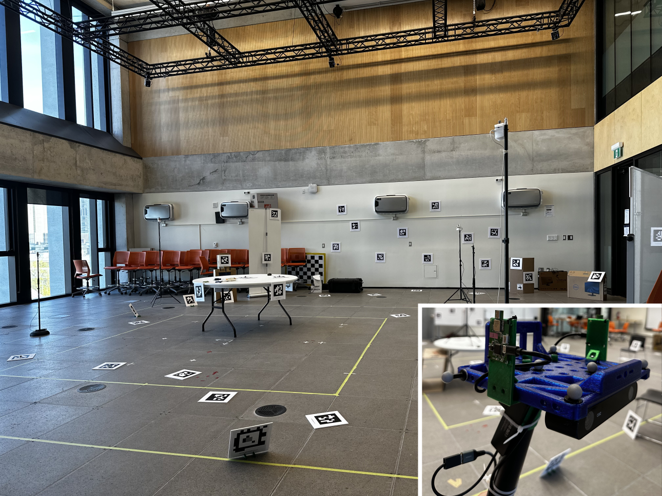
Figure 1. The STAR-loc dataset contains data collected on different trajectories of a sensor rig (bottom right) in a Vicon mocap arena, providing range and calibrated stereo measurements.

• data/<dataset-name>/: folder containing all data of the run of name <dataset-name> (see Section 3 for an overview of the different runs).

  • csv files of processed data (apriltag.csv, imu.csv, uwb.csv, gt.csv. See data/README.md for information on the data fields.

  • calib.json: file with calibration information of this run.

  • (Drive only) bag files of this run (<dataset-name>_0.db3 and metadata.yaml)

  • (Drive only) some analysis plots of the data, see Appendix A for information on the plots.

  • (Drive only) the video of the left camera with overlaid Apriltag detections.

• mocap/: folder containg environment information.

  • uwb_markers_<version>.csv,mocap/environment_<version>.csv: csv files of the UWB anchor and Apriltag landmark locations, respectively, used in Setup of <version>. See Section 3 for descriptions of the different setup versions.

  • (Drive only) plots of the different setup versions.

  • (Drive only) vsk and tag config files used in calibration procedure.

2. System description

A photo of the sensor rig used for data collection is shown in Figure 2. Attached to the rig are the UWB tag(s) and the stereo camera. A laptop (not shown) is used for driving all sensors and collecting the data through the help of dedicated Robot Operating System (ROS) nodes.

Figure 2 also depicts the different sensor frames including their transforms. The frames are:

• $\mathcal{F}_{r}$: robot frame (tracked by mocap system)

• $\mathcal{F}_{c}$: camera frame

• $\mathcal{F}_{t_{i}}$: $i$-th tag frame, with $i=1\ldots 3$

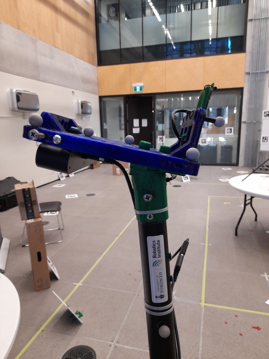
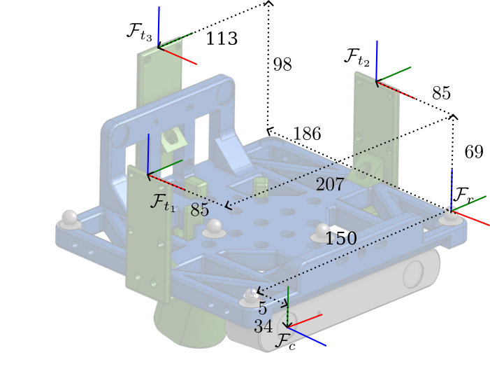
Figure 2. Left: the used sensor rig with one UWB tag and stereo camera attached. Right: the corresponding CAD model including the definitions of the sensor frames, showing the three possible UWB tag locations $\mathcal{F}_{t_{1}}$, $\mathcal{F}_{t_{2}}$ and $\mathcal{F}_{t_{3}}$ and the stereo camera frame $\mathcal{F}_{c}$.

2.1. UWB tag and anchors

The main UWB system used are custom-made boards provided by the Mobile Robotics and Autonomous Systems Laboratory (MRASL), where each board is fitted with DWM1000 UWB transceivers. The board is shown in Figure 6. These boards are equipped with a STM32F405RG microcontroller to interface with the DWM1000 modules, and the boards are then connected to the onboard computer using USB. Details about the ranging and communication protocols can be found in uwb-hardware . We also provide a small dataset with the off-the-shelf development kit MDEK1001 (setup s5). We use custom data collection scripts to record distance measurements.

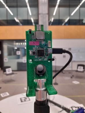
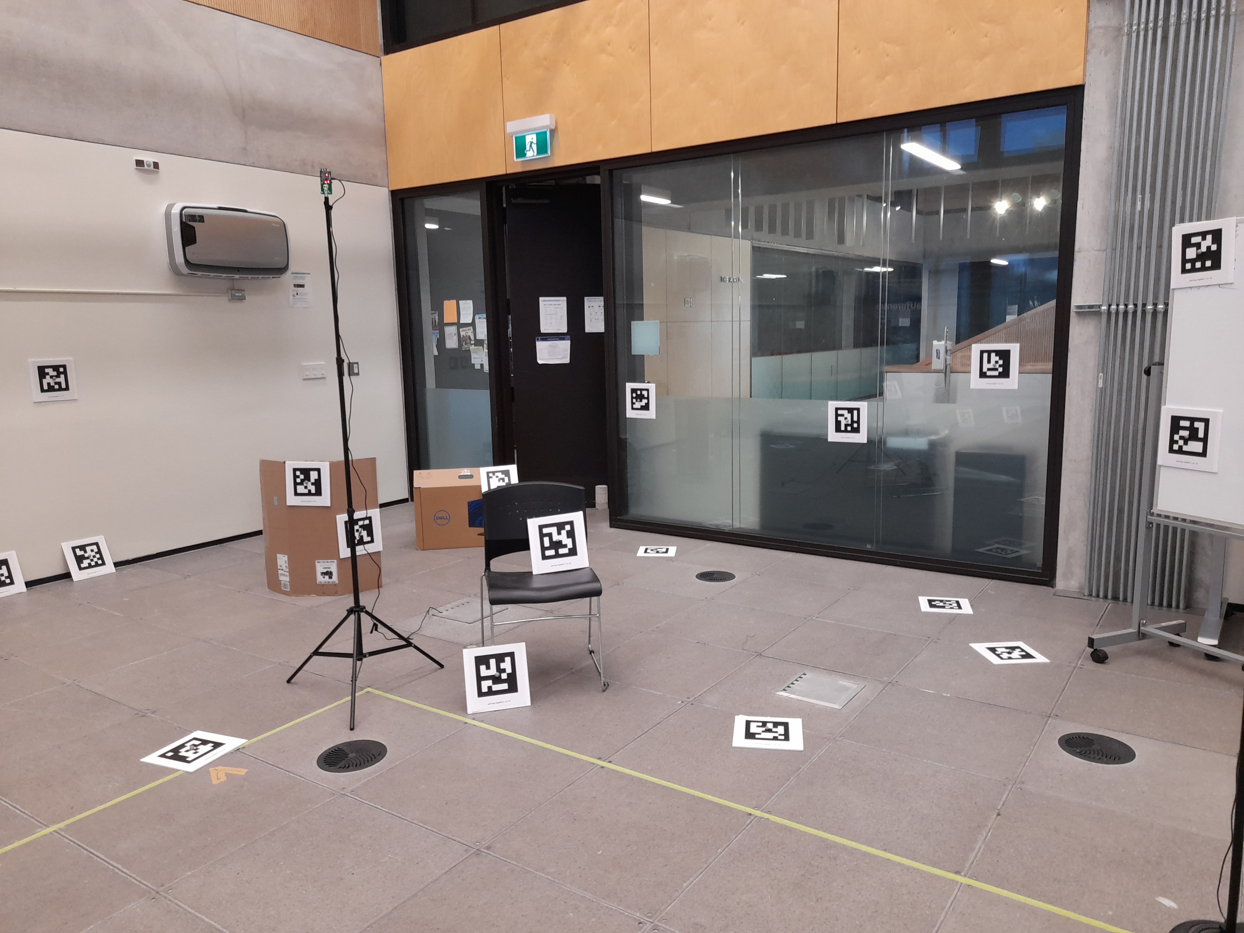
Figure 3. Left: One of eight fixed UWB anchors. Right: subset of Apriltag landmarks.

2.2. Visual landmarks

We use Apriltags apriltag , tag version Tag36h11, as known landmarks. The tags are printed on US letter paper, glued to foam board, and spread throughout the room at fixed locations of different heights and orientations, as shown in Figure 6. We use the open-source libraries apriltag_ros and apriltag_msg for Apriltag detection.

2.3. Stereo camera

We use the ZED2i stereo camera from stereolabs with a $12\text{\,}\mathrm{c}\mathrm{m}$ baseline and set to $1920\times 1080$ resolution. For data collection, we employ the ROS-based camera driver provided by stereolabs, using the image_transport_plugins ROS packages for image compression.

2.4. Motion capture

We use a VICON mocap system for ground truth monitoring. For data collection, we use the ros2-vicon-receiver package by OPT4SMART to publish the native data stream from VICON as ROS messages.

3. Dataset overview

Table 1. Overview of datasets

setup	s1	s2	s3	s4	s5
landmarks	v1	v1	v2	v2	v3
trajectory						description
loop-2d	x	x	x	x	x	multiple loops, keeping sensor rig level
loop-2d-fast	x	x	x			multiple loops, walking fast, keeping sensor rig level
loop-3d	x	x	x		x	multiple loops, pointing sensor rig at different directions
zigzag		x	x	x		a roughly piecewise linear trajectory, keeping sensor rig level
eight		x	x			draw large eights in the air, pointing at an area dense in Apriltags
apriltag			x			one loop with complete Apriltag detections
ell			x			multiple ell-shaped trajectories with a lot of height variation
grid			x			static measurements at 8 grid points, including one full circle at last point.
loop-3d-z			x			loop with a lot of height variation

3.1. Runs and setups

An overview of all collected datasets is shown in Table 1. The datasets are distinguished by their setup, landmarks and trajectory version. These aspects are described in more details in the paragraphs below.

Trajectory versions

loop-2d

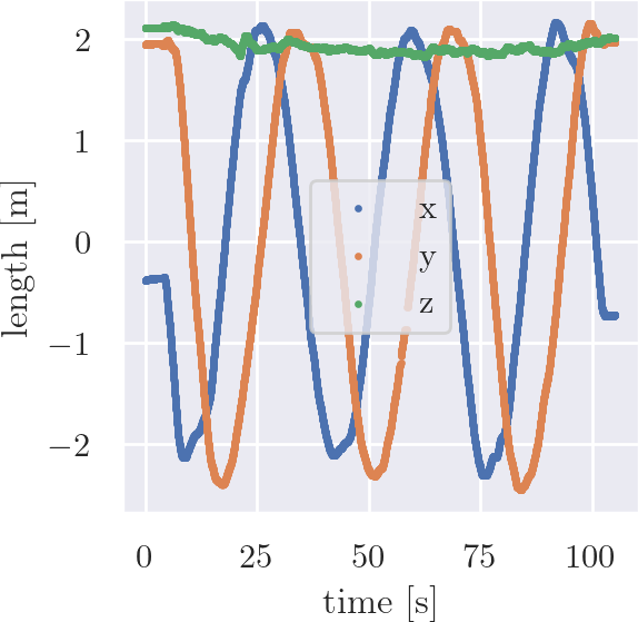
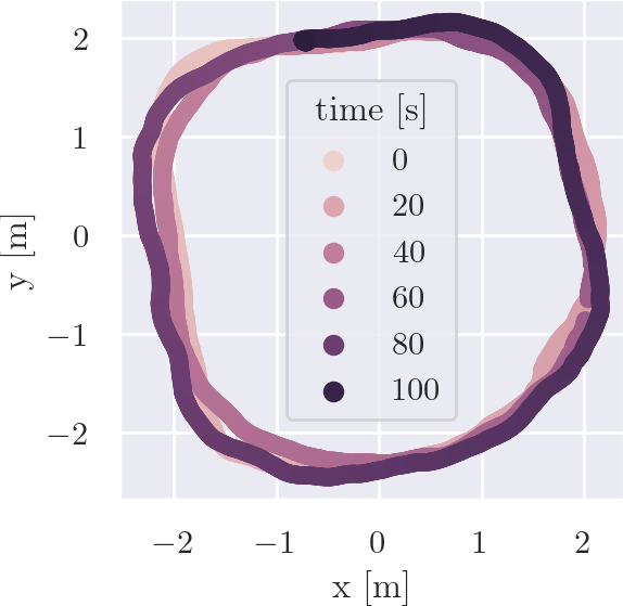
loop-2d-fast

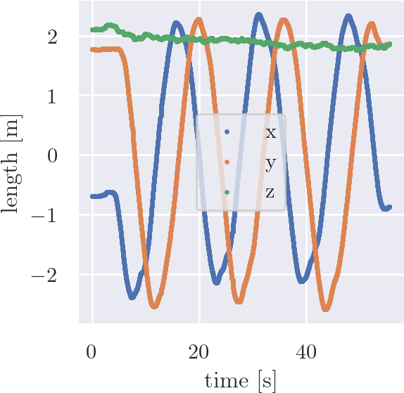
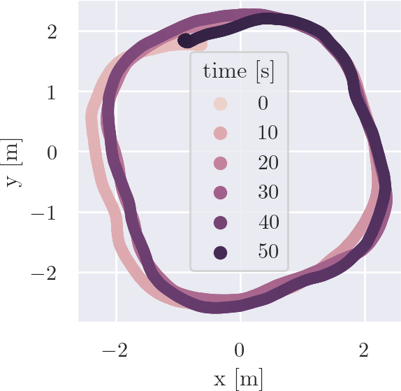
loop-3d

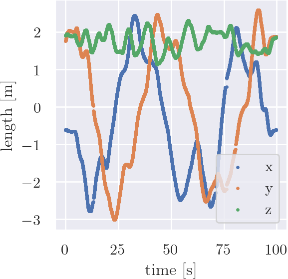
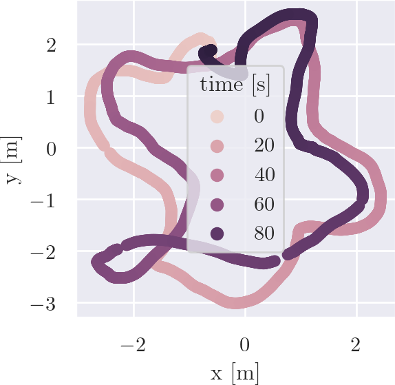
zigzag

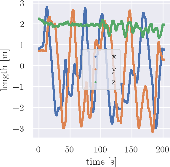
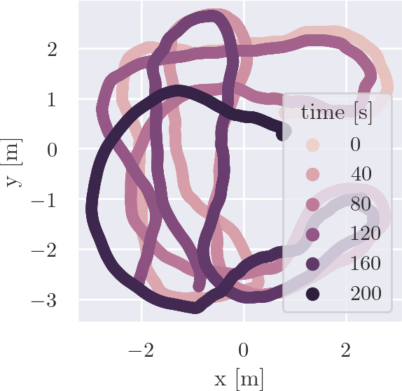
eight

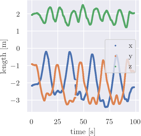
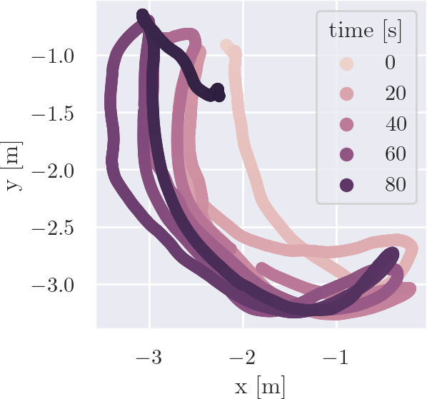
Figure 4. Overview of the different standard trajectory types recorded with many different setups. The shown data corresponds to setup s3.

apriltag

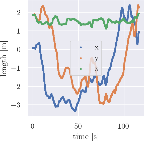
ell

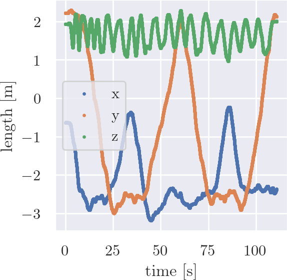
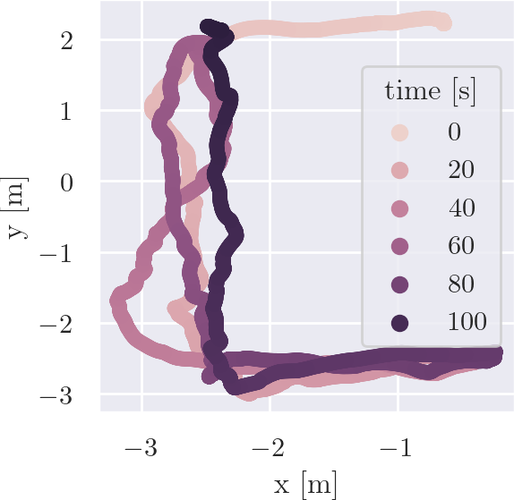
grid

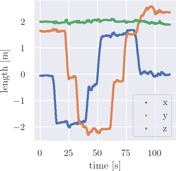
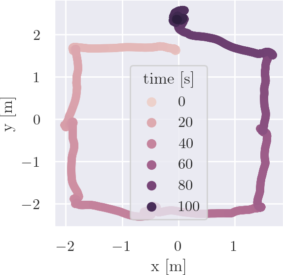
loop-3d

Figure 5. Overview of the trajectory types recorded with the setup s3.

The first five listed trajectory types (also denoted “standard” in what follows) are repeated for different kinds of tag setups to facilitate their comparison. The four remaining datasets are recorded for setup s3 only, and serve as datasets to highlight specific phenomena. Example trajectories for the 5 standard dataset types are shown in Figure 4.

An overview of the remaining datasets is shown in Figure 5.

Setup versions

The datasets include 5 different setups of the sensor rig:

• s1: We use locations 1 and 2 (see Figure 2) for the UWB tags 1 and 2, respectively, on the sensor rig. The rig is held just above the person’s height using a single PVC tube.

• s2: hand-held up, 2 tags: The sensor rig is mounted on a second PVC tube to increase the proportion of line-of-sight (LOS) regions: the rig is now a half metre above the person’s height.

• s3: hand-held up, 1 tag: We use only location 3 (see Figure 2) for the UWB tag 1.

• s4: mounted on Jackal robot, 1 tag at location 3.

• s5: hand-held up, 1 Decawave tag at location 3.

Landmarks versions

The datasets include three different landmark layouts. The first two differ only minimally in geometry; Version v2 is an improved setup of v1 after analyzing noise patterns of both the mocap system and the UWB anchors. Version v3 is the layout used for Decawave data and consists of only four anchors. The different layouts are shown Figure 6.

v1

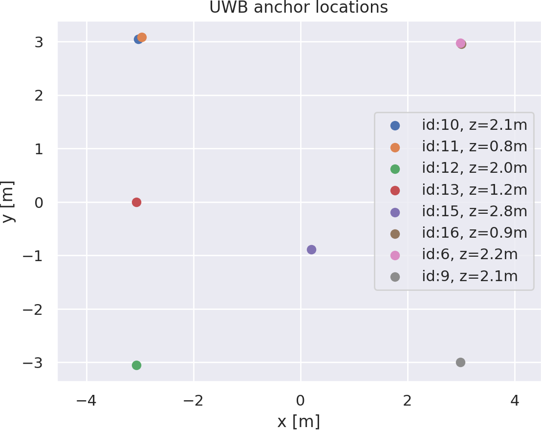
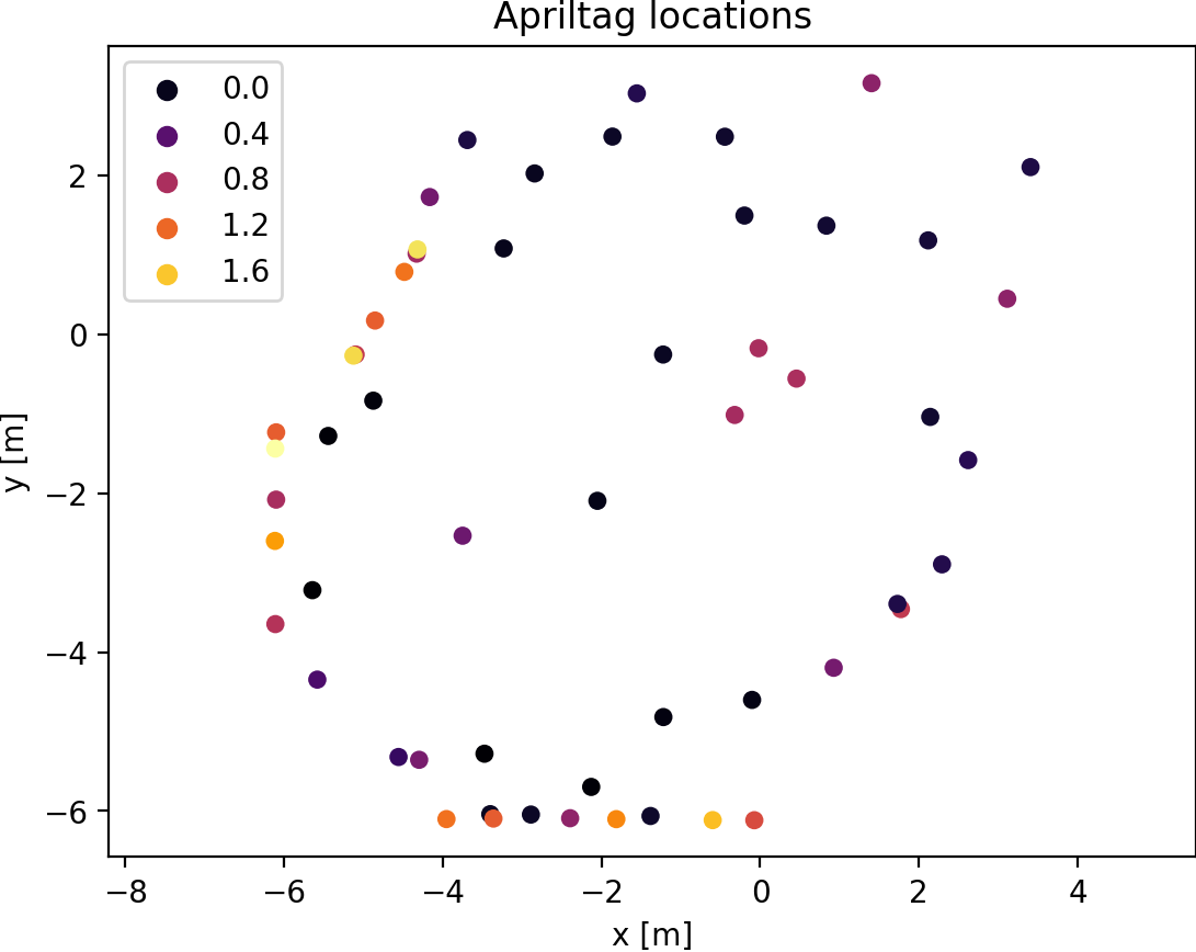
v2

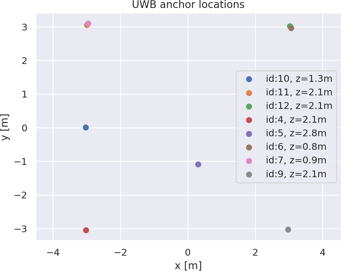
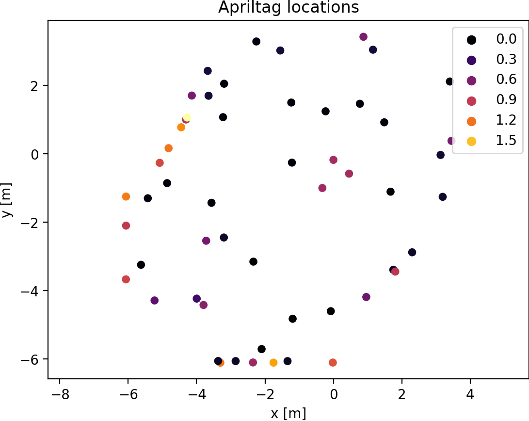
v3

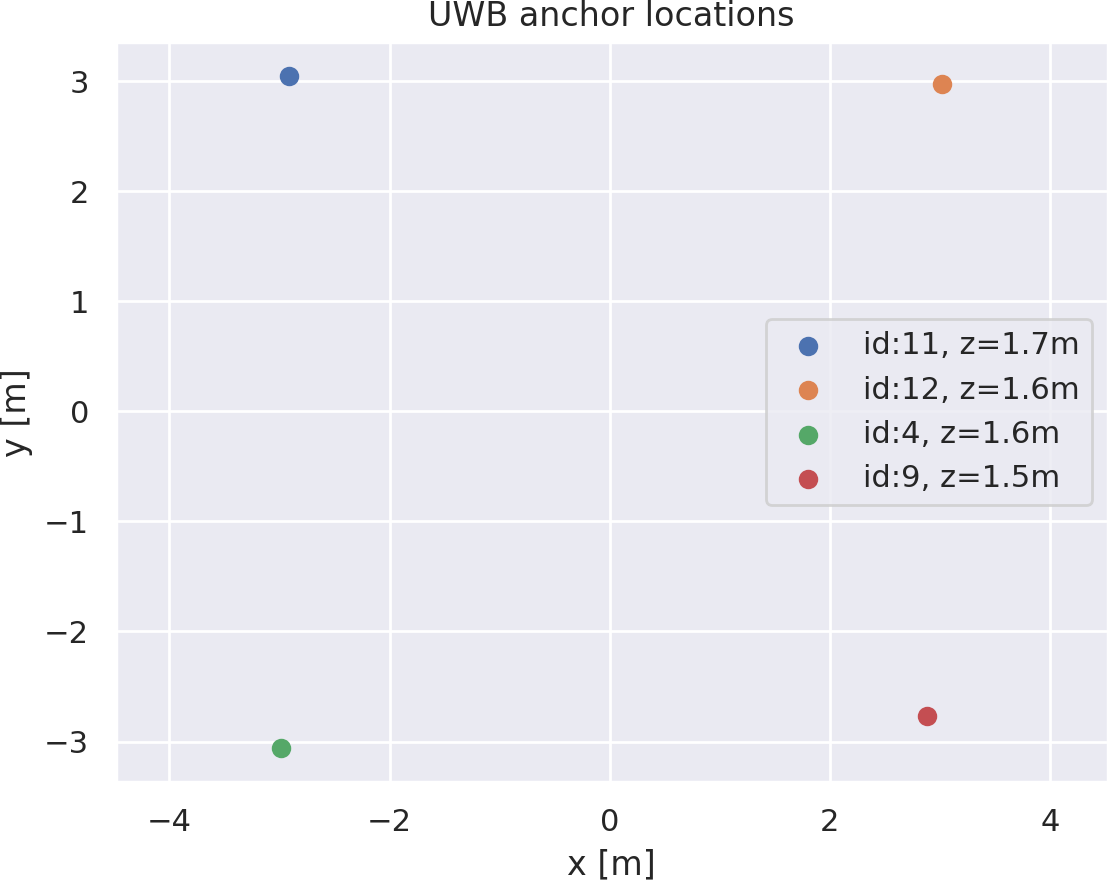
Figure 6. The three different UWB anchor layouts and two different Apriltag landmark layouts used.

3.2. Collected data

In this Section, we report some statistics taken over all the collected datasets. An individual analysis per dataset can be found in Appendix A. The names of the datasets are of the format:

$$\texttt{trajectory-version\_setup-version}.$$

Number of messages and rates

The collected data rates and number of messages received, for each dataset, are shown in Table 2.

Table 2. Overview of all collected datasets

	median rate [Hz]				duration [s]
data type	Apriltag	UWB	Vicon	IMU
loop-2d_s1	14.9	266.1	48.0	193.8	65.6
loop-2d-fast_s1	14.9	260.7	48.0	194.1	34.2
loop-3d_s1	14.9	249.3	48.0	193.6	87.7
loop-2d_s2	14.9	251.3	48.0	193.3	86.9
loop-2d-fast_s2	14.9	246.4	48.1	192.8	35.3
loop-3d_s2	14.9	244.6	48.0	192.6	80.3
zigzag_s2	14.9	256.4	48.0	193.0	78.0
eight_s2	15.0	246.6	48.1	192.3	49.2
loop-2d_s3	14.9	248.6	48.0	192.9	105.3
loop-2d-fast_s3	14.9	247.8	48.0	193.1	55.5
loop-3d_s3	14.9	249.4	48.0	193.9	99.8
zigzag_s3	14.9	249.4	48.0	193.9	201.6
eight_s3	14.9	247.4	48.0	192.9	98.5
loop-2d_s4	11.3	247.4	48.3	196.2	194.1
zigzag_s4	14.3	249.1	48.0	198.0	218.2
grid_s3	14.9	248.6	48.0	192.7	112.9
ell_s3	14.9	248.7	48.0	192.6	111.1
loop-3d-z_s3	14.9	249.1	48.0	193.2	150.3
apriltag_s3	14.9	247.8	48.0	193.1	116.4
loop-2d_s5	14.9	40.0	48.0	193.2	82.0
loop-2d-v2_s5	14.9	40.0	48.0	193.6	101.0
loop-3d_s5	14.9	40.0	48.0	193.1	67.0
median rates [Hz]	14.9	248.6	48.0	193.2

UWB quality

The quality of UWB measurements per dataset, measured by the (signed) difference between the ground truth and measured distances, is shown in Figure 7. The measurements shown are before calibration. For performance after calibration, please refer to the individual dataset plots provided in the dataset on Google Drive.

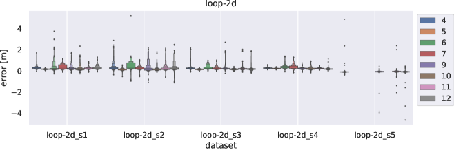
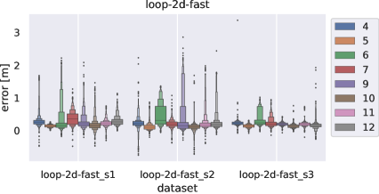
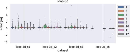
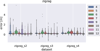
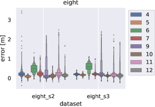
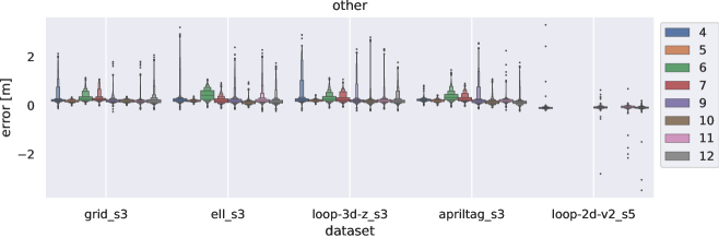
Figure 7. UWB performance over all datasets.

Stereo quality

The quality of stereo measurements per dataset is measured by the difference between the projected pixel values using the ground truth landmark locations and camera pose, and the measured pixel values, as shown in Figure 8. The measurements shown are before calibration.

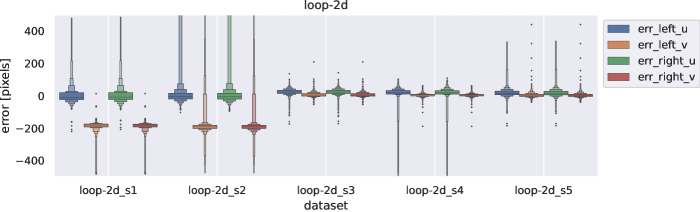
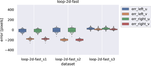
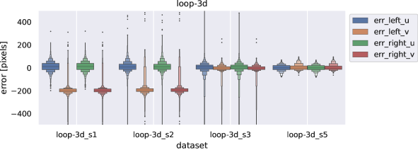
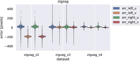
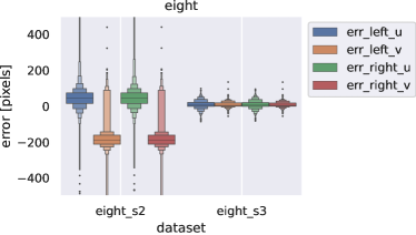
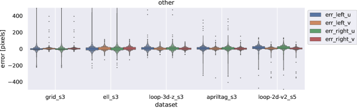
Figure 8. Stereo camera performance over all datasets.

4. Data processing

4.1. Stereo camera calibration

Stereo camera calibration involves two main steps:

1. Data association: Involves associating Apriltag identifiers to the ground truth Vicon locations.

2. Extrinsic calibration: Involves solving for the transformation between the Vicon frame attached to the camera rig and the left Zed2i camera frame (at focal point).

Note that the rectified intrinsic parameters provided for the Zed2i camera were assumed to be accurate and were not tuned in this calibration procedure.

Data association was performed using a camera sequence with Apriltaglabels to manually label the set of Vicon ground truth landmark locations.

For extrinsic calibration, we provide three different methodologies: fixed calibration (appendix _cal), global calibration (_cal_global) and individual calibration (_cal_individual) For fixed calibration, the CAD model of the sensor rig was used to establish a transformation between Vicon and camera frames. For global calibration, we use the dataset apriltag_s3 to find the transformation that minimizes the reprojection (also called photometric) error using Gauss-Newton optimization state-estimation . For individual calibration, we use the same procedure, but calculate the best transformation for each dataset individually.

To reduce the effect of outliers, we perform the calibration three times, removing outliers after each iteration. Outliers are pixel measurements with errors higher than a fixed threshold (we used 100 for v2 and v3 and 300 for v1).

4.2. UWB calibration

The ranging protocol used in these experiments is the double-sided two way ranging (DS-TWR) protocol shown in Figure 9. Each of the 6 timestamps $t_{i},i\in\{1,\ldots,6\}$ is recorded as part of the dataset, as well as the received signal power at the timestamps $t_{2}$ and $t_{4}$.

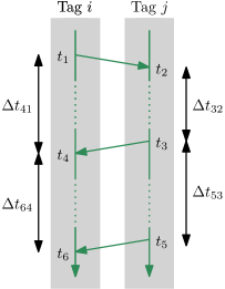
Figure 9. The DS-TWR protocol used in the experiments to generate range measurements between any two UWB tags.

A time-of-flight measurement can be generated from the recorded timestamps as

$$t_{f}=\frac{1}{2}\left(\Delta t_{41}-\frac{\Delta t_{64}}{\Delta t_{53}}\Delta t_{32}\right),$$

where, as shown in Figure 9, $\Delta t_{ji}=t_{j}-t_{i}$. Nonetheless, the range measurements are biased as shown in the blue distribution in Figure 11. This error stems from multiple factors such as timestamping inaccuracies, multipath propagation, and obstacles.

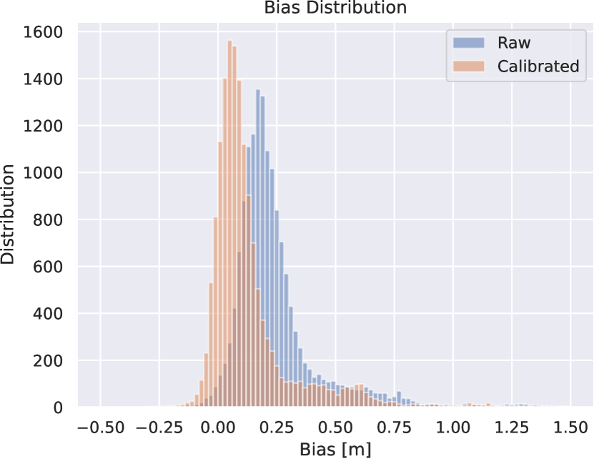
Figure 10. Histogram representing the distribution of the bias of the range measurements for the zigzag s2 experiment. The distribution for the raw and the calibrated measurements are shown.

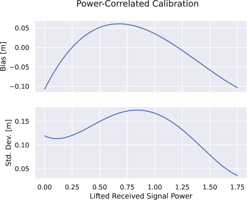
Figure 11. The relation between the bias and the standard deviation of the bias for the measurements as a function of the lifted received signal power. These are obtained from a separate calibration experiment.

Table 3. Calibrated antenna delays for all tags using a separate calibration experiment.

Tag ID	Antenna Delay [ns]
1	-0.5672
2	-0.2139
3	-0.2499
4	-0.5514
5	-0.3756
6	-0.3292
7	-0.1349
9	-0.2914
10	-0.3000
11	-0.3953
12	-0.3069

To obtain more accurate range measurements, the calibration procedure presented in shalaby2023 is implemented. The antenna delay values shown in Table 3 and the power-to-bias relation shown in Figure 11 are obtained by performing two separate experiments with 6 UWB tags fitted on 3 flying quadcopters (2 per quadcopter). A relation between the uncertainty or standard deviation of measurements as a function of the received signal power is also learned and is shown in the bottom plot of Figure 11. More information on the experiment and how these relations are obtained can be found in shalaby2023 .

The timestamps are then corrected using the antenna delays and the received-signal power and the range measurements are recomputed, giving much less biased measurements as shown in Figure 11. Both the raw and calibrated measurements are provided when available, and they can be found under the columns range and range_calib, respectively. The uncertainty of each measurement is also provided under the std column.

5. Acknowledgments

We would like to thank Joey Zou for his help in preparing the Decawave data collection pipeline and rig adjustments. We also thank Connor Jong for his help during experiments and Abhishek Goudar for advice on UWB data collection.

Appendix A Individual dataset plots

Each dataset folder in data/<dataset_name> contains a number of plots for fast data inspection. The different plots are described in more detail below.

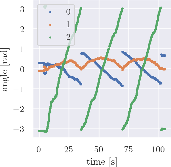
Figure 12. Ground truth data, from left to right: projection of trajectory to x-y plan (gt-xy.png), translation over time (gt-t-xyz.png) and rotation over time, using axis-angle representation (gt-t-angles).

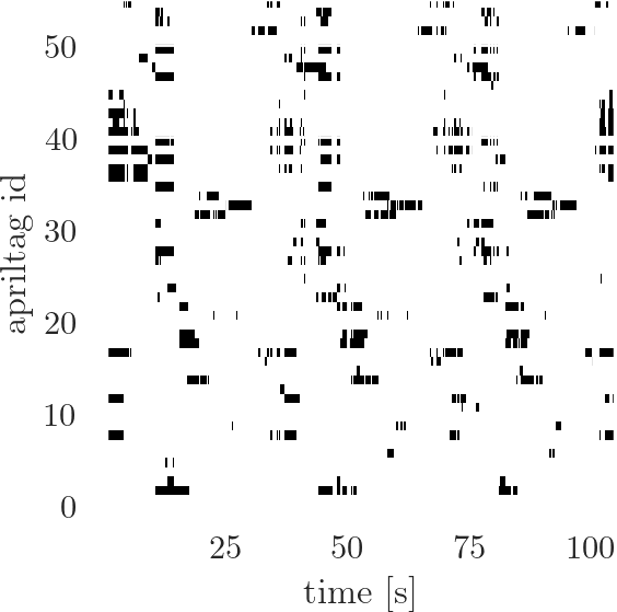
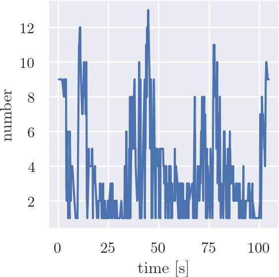
Figure 13. Apriltag data, from left to right: mask of Apriltag detections over time (apriltag_mask.png), black corresponding to at least one detection in either the left or the right stereo camera frame, and number of synchronized Apriltag detections over time (apriltag_number.png).

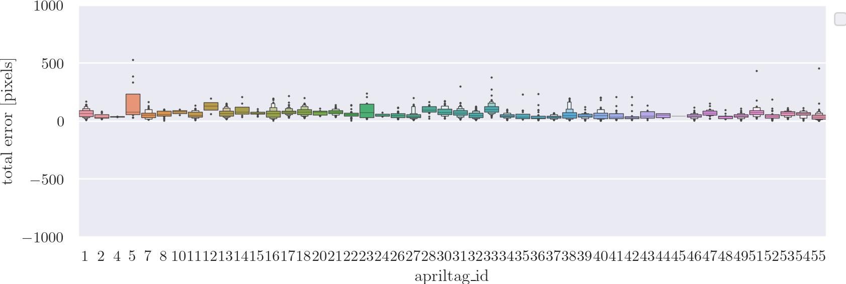
Figure 14. Stereo camera pixel errors, using no calibration (top, apriltag_cal.pdf), one global calibration (middle, apriltag_cal_global.pdf) and individual calibrations (bottom, apriltag_cal_individual.pdf). We also provide plots cropped at $\pm$ 300 pixels (_crop).

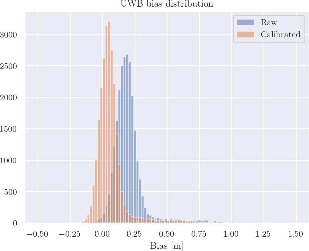
Figure 15. UWB data, top: UWB bias before and after calibration (uwb_bias_histogram.png), bottom: raw and calibrated measurements compared to ground truth (uwb_measurements_tag_1.png).

References

- (1) Mohammed Ayman Shalaby, Charles Champagne Cossette, James Richard Forbes, and Jerome Le Ny, “Calibration and Uncertainty Characterization for Ultra-Wideband Two-Way-Ranging Measurements,” arXiv:2210.05888, 2022.
- (2) Edwin Olson, “AprilTag: A robust and flexible visual fiducial system,” in 2011 IEEE International Conference on Robotics and Automation, 2011, pp. 3400-3407, doi: 10.1109/ICRA.2011.5979561.
- (3) Mohammed Ayman Shalaby, Charles Champagne Cossette, Jerome Le Ny, and James Richard Forbes.“Multi-Robot Relative Pose Estimation and IMU Preintegration Using Passive UWB Transceivers,” arXiv:2304.03837, 2023.
- (4) Barfoot, Timothy D. State Estimation for Robotics. Cambridge University Press, 2017.