Median Surface Brightness Profiles of Lyman-$\alpha$ Haloes in the MUSE Extremely Deep Field

We present the median surface brightness profiles of diffuse Ly$\alpha$ haloes (LAHs) around star-forming galaxies by stacking 155 spectroscopically confirmed Ly$\alpha$ emitters (LAEs) at $3<z<4$ in the MUSE Extremely Deep Field (MXDF), with median Ly$\alpha$ luminosity $\mathrm{L_{Ly\alpha}\approx 10^{41.1}erg\,s^{-1}}$. After correcting for a systematic surface brightness offset we identified in the datacube, we detect extended Ly$\alpha$ emission out to a distance of $\approx$270 kpc. The median Ly$\alpha$ surface brightness profile shows a power-law decrease in the inner 20 kpc, and a possible flattening trend at larger distance. This shape is similar for LAEs with different Ly$\alpha$ luminosities, but the normalisation of the surface brightness profile increases with luminosity. At distances larger than 50 kpc, we observe strong overlap of adjacent LAHs, and the Ly$\alpha$ surface brightness is dominated by the LAHs of nearby LAEs. We find no clear evidence of redshift evolution of the observed Ly$\alpha$ profiles when comparing with samples at $4<z<5$ and $5<z<6$. Our results are consistent with a scenario in which the inner 20 kpc of the LAH is powered by star formation in the central galaxy, while the LAH beyond a radius of 50 kpc is dominated by photons from surrounding galaxies.

1 Introduction

Galaxies are born and bred in their gaseous haloes (e.g. Tumlinson et al., 2017). Within the circumgalactic medium (CGM), gas and metals can be ejected from galaxies by feedback processes or stripping, or they can be (re-)accreted to fuel star formation. On larger scales, the intergalactic medium (IGM) traces the cosmic web of matter that connects, forms and fuels galaxies, and its properties may be changed by feedback processes. Mapping the gas distribution in the IGM and the CGM, and investigating their relationship with the interstellar medium (ISM) of the galaxies are crucial for understanding the evolution of galaxies.

The hydrogen Ly$\alpha$ line is a powerful tool for mapping the CGM and IGM at high redshift (e.g. Steidel et al., 2011; Ouchi et al., 2020; Bacon et al., 2021). Theoretical studies predict substantial amounts of neutral hydrogen in the CGM and IGM (e.g. Fumagalli et al., 2011; van de Voort et al., 2012), and this has been observed through absorption measurements (e.g. Lee et al., 2018; Newman et al., 2020). The Ly$\alpha$ photons are produced by hydrogen recombination following ionization, or by collisional excitation following photo- or shock- heating. As they propagate through the ISM, CGM and IGM, they can be repeatedly absorbed and re-emitted by the neutral hydrogen gas. This resonant nature of Ly$\alpha$ makes it a unique tracer of neutral gas distribution, though the likelihood of it being absorbed by galactic dust is non-negligible. In addition to its utility in mapping the hydrogen gas, the Ly$\alpha$ emission line is also a highly informative probe of high-redshift star-forming galaxies (e.g. Ouchi et al., 2008; Shibuya et al., 2012; Guo et al., 2020a; Bacon et al., 2023). It is intrinsically the strongest emission line in the rest-frame UV/optical spectrum (e.g. Partridge & Peebles, 1967). Therefore, observing the large-scale spatial distribution of Ly$\alpha$ emission can provide a map of the large-scale structure of the early Universe, e.g., the pristine gas distribution as well as the distribution of high-redshift galaxies.

In the past decades, extended Ly$\alpha$ emissions, known as Ly$\alpha$ haloes (LAHs), have been observed around Ly$\alpha$ emitting galaxies (LAEs) at $\mathrm{z\gtrsim 2}$ using the narrow band (NB) technique (e.g. Matsuda et al., 2012; Feldmeier et al., 2013; Momose et al., 2014, 2016; Xue et al., 2017; Wu et al., 2020; Kikuta et al., 2023) and integral field unit (IFU) facilities (e.g. Wisotzki et al., 2016; Leclercq et al., 2017; Daddi et al., 2021; Kusakabe et al., 2022). The LAHs have also been observed in the local Universe in the vicinity of galaxies (e.g. Hayes et al., 2013; Duval et al., 2016). The LAHs have physical scales of several tens of kpc, where most important processes regulating galaxy formation and evolution occur. By combining deep exposures and stacking, recent studies have expanded the detection of extended Ly$\alpha$ emission to hundreds of kpc (e.g. Kakuma et al., 2021; Kikuchihara et al., 2022; Lujan Niemeyer et al., 2022b, a). Despite the substantial observational work on the spatial content of the LAHs, the physical mechanisms of the production and propagation of Ly$\alpha$ photons are still under debate (e.g. Cantalupo et al., 2005; Zheng et al., 2011; Rosdahl & Blaizot, 2012; Byrohl et al., 2021).

The ESO-VLT instrument MUSE (the Multi Unit Spectroscopic Explorer, Bacon et al., 2010) revolutionized the observation of the CGM and IGM. This IFU facility with a large field of view is highly efficient in mapping the extended emission from the CGM, or even the IGM, using multiple tracers, e.g., Ly$\alpha$ (e.g. Wisotzki et al., 2016, 2018; Cai et al., 2017, 2019; Leclercq et al., 2017, 2020; Gallego et al., 2018, 2021; Claeyssens et al., 2019, 2022; Bacon et al., 2021; Kusakabe et al., 2022), C IV, He II, C III] (e.g. Borisova et al., 2016; Guo et al., 2020b), Mg II (e.g. Zabl et al., 2021; Leclercq et al., 2022), and [O II] (e.g. Johnson et al., 2022). At $z\gtrsim 3$, MUSE observations have identified large samples of individual LAEs, and allowed for the analysis of the surface brightness profiles of the LAHs individually or by stacking. Wisotzki et al. (2018) find that the LAHs on average extend to tens to hundreds kpc, thus covering nearly all of the sky by projection. Bacon et al. (2021) detect the cosmic web in Ly$\alpha$ emission on scales of several comoving Mpc. Kusakabe et al. (2022) study the LAHs around UV-selected galaxies instead of objects selected from their Ly$\alpha$ emission. The existence of extended Ly$\alpha$ emission around non-LAEs implies a significant amount of neutral hydrogen in the CGM of the normal star-forming galaxies. The deep MUSE observations have also allowed for the spatially resolved spectroscopic analysis of a sample of bright individual LAHs (e.g. Claeyssens et al., 2019; Leclercq et al., 2020).

In this work, we measure the median Ly$\alpha$ surface brightness profile of 369 spectroscopically confirmed LAEs at $3<z<6$, with our primary focus being $3<z<4$. The current dataset is 5-14 times deeper than that of Wisotzki et al. (2018). We therefore expect to expand the detection of extended Ly$\alpha$ emission out to hundreds of kpc from the LAE center. Previous studies have suggested that the dominant origin of the LAHs differs at different radii relative to the galaxies (e.g. Lake et al., 2015; Mitchell et al., 2021; Byrohl et al., 2021). By measuring the Ly$\alpha$ profiles out to large radii, we expect to provide more constraints on the origin of the LAHs at different distances.

The paper is organized as follows: we describe the definition of the LAE sample and our data reduction in Section 2. Section 3 provides the results, highlights the median Ly$\alpha$ surface brightness profile at $3<z<4$, and presents the profiles of different subsamples and datasets. In Section 4 we discuss our results by comparing with previous observations and theoretical predictions, and also interpret the Ly$\alpha$ profiles from the point of view of cross-correlation functions. We summarize in Section 5.

We adopt the standard $\mathrm{\Lambda CDM}$ cosmology with $H_{0}\mathrm{=70\,km\,s^{-1}\,Mpc^{-1}}$, $\mathrm{\Omega_{m}=0.3}$ and $\mathrm{\Omega_{\lambda}=0.7}$. All distances are proper, unless noted otherwise.

2 The galaxy sample and data analysis

This work is based on the data release 2 (DR2) of the MUSE Hubble Ultra Deep Field surveys (Bacon et al., 2023). The DR2 data consists of 3 datasets, a $\mathrm{3\times 3}$ arcmin² mosaic of 9 MUSE fields at 10-hour depth (hereafter MOSAIC), a $\mathrm{1\times 1}$ arcmin² field at 31-hour depth (hereafter UDF-10), and the MUSE eXtremely Deep Field (MXDF), with a diameter of 1 arcmin and the deepest achieved exposure of 141 hours. In this work, we mainly use the MXDF. It is the deepest spectroscopic survey ever performed, reaching an unresolved emission line median $\mathrm{1\sigma}$ surface brightness limit of $\mathrm{<10^{-19}\,erg\,s^{-1}\,cm^{-2}\,arcsec^{-2}}$. The MOSAIC dataset, which covers an area approximately nine times larger than the MXDF but has an exposure time approximately 14 times shorter, is a useful comparison dataset. In Section 3.4, we describe our efforts to detect more extended emission in MOSAIC. For further details on the data reduction of the MXDF and MOSAIC, we refer the reader to Bacon et al. (2023).

2.1 The LAE sample

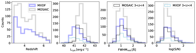
Figure 1: Distribution of the redshift (first panel), Ly$\alpha$ luminosity (second panel), Ly$\alpha$ line rest-frame FWHM (third panel) and S/N of Ly$\alpha$ line (fourth panel) of the LAE sample. The thick lines present the distributions of the whole galaxy samples in MXDF (blue lines) or MOSAIC (grey lines). The narrow lines show the LAEs at $3<z<4$, the redshift range of most interest for this work.

Bacon et al. (2023) perform a meticulous work that involves multiple cross-checked procedures to achieve a high-quality and homogeneous source detection. Their final catalogue provides the redshifts, multi-band photometries, morphological and spectral properties, as well as measurements of stellar mass and star formation rate of all the galaxies discovered in the MOSAIC, UDF-10 and MXDF fields. The MXDF field contains a total of 369 LAEs at $3<z<6$, while MOSAIC contains 693 detected LAEs. In this work, we focus on the redshift range of $3<z<4$. In this redshift range, the efficiency of MUSE is high, the redshift dimming is low, there are no strong OH sky line, enabling us to acquire a highly representative LAE sample that extends to very low Ly$\alpha$ luminosity. In the redshift range $3<z<4$, there are 155 LAEs detected in MXDF and 329 in MOSAIC.

Figure 1 shows the distribution of redshift, Ly$\alpha$ luminosity ($\mathrm{L_{Ly\alpha}}$), rest-frame Ly$\alpha$ line FWHM and Ly$\alpha$ line S/N for all LAEs and for the sample at $3<z<4$. All these quantities are derived from Bacon et al. (2023). The median Ly$\alpha$ luminosity of LAEs at $3<z<4$ in the MXDF is $\mathrm{L_{Ly\alpha,median}\approx 10^{41.1}erg\,s^{-1}}$. Their median stellar mass is $\mathrm{M_{*}\approx 10^{7.6}M_{\odot}}$. The median Ly$\alpha$ S/N for LAEs at $3<z<4$ in the MXDF is 7.7, with the 95th percentile of 53.4 and the 5th percentile of 2.9. According to Herrero Alonso et al. (2023), the typical halo mass for MXDF LAEs over the whole redshift range of is $\mathrm{log(M_{h}/[h^{-1}M_{\odot}])=10.77^{+0.13}_{-0.15}}$. The number should be smaller for MXDF LAEs at $3<z<4$, as their typical Ly$\alpha$ luminosity is lower than their parent sample (second panel of Figure 1).

We try to avoid contamination from the bright AGNs that can be dominant in powering the extended Ly$\alpha$ emission. Given the sky coverage of MXDF and MOSAIC (1-3 arcmin), the possibility of detecting a substantial number of AGNs is very low. There is one type-I AGN at $z$=3.2. There is another type-II AGN at $z$=3.06 that is cross-matched by the Chandra Chandra 7Ms catalog (Luo et al., 2017). Both AGNs are found in MOSAIC (Bacon et al., 2023), and are excluded from our analysis. Considering that the LAEs in our sample have Ly$\alpha$ luminosity $\mathrm{L_{Ly\alpha}<10^{43}erg\,s^{-1}}$, the AGN contamination should be very low (e.g. Sobral et al., 2018; Calhau et al., 2020; Zhang et al., 2021). According to the estimation of Zhang et al. (2021), the AGN fraction at $\mathrm{L_{Ly\alpha}<10^{43}erg\,s^{-1}}$ is $\lesssim$ 0.05.

2.2 Masking and continuum subtraction

The exposure of the MXDF field is not uniform, with the integration time decreasing from 141 hours at the field centre to several hours at the edge of the field (Bacon et al., 2023). We mask out the area with exposure time smaller than 110 hours to keep a high S/N and a more homogeneous sample throughout the selected FoV. We also mask the wavelength slices affected by bright sky lines to avoid strong sky line residuals. We remove the continuum by performing a spectral median filtering using a wide spectral window of 200 Å. This approach provides a rapid and effective way to remove continuum sources in the search for extended line emission.

We focus on detecting the extended Ly$\alpha$ line at large distances from the LAEs. To achieve this focus, we need to remove the contamination from emission and absorption lines from foreground galaxies and from the LAEs themselves. We mask out all the detected emission and absorption lines from all the galaxies in the continuum-subtracted datacube, with the exception of the Ly$\alpha$ line. The mask is based on the composite segmentation images provided by Bacon et al. (2023). The segmentation images are provided by SExtractor (Bertin & Arnouts, 1996), with a S/N limit of 2.

Note that in case that more than one LAE exists in one NB, we keep all the objects. In Section 3.2, we will demonstrate that as the exposure becomes deeper and the distance increases, neighboring LAEs inevitably appear within the field of view. Therefore, in Section 3.2, we will also present an additional measurement after removing the neighboring LAEs.

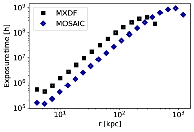
Figure 2: The stacked exposure time in each radial bin for LAEs at $3<z<4$. The black and blue symbols show the MXDF and MOSAIC sample, respectively

2.3 Extraction of Ly$\alpha$ surface brightness

We construct the pseudo-NB image for each LAE based on the MUSE datacube. Each NB is centered on the peak wavelength of the Ly$\alpha$ line. In the case of Ly$\alpha$ lines with two peaks, we center the NB on the red peak. The spectral bandwidth of the Ly$\alpha$ NB is fixed at 12 cMpc, which corresponds to approximately 15.0 Å (in the observational frame) or 924.4 km/s at $z\approx 3$, and 34.3 Å or 1206.4 km/s at $z\approx 6$. This bandwidth is chosen to include most of the Ly$\alpha$ flux, providing a reasonable tolerance for the variety of Ly$\alpha$ line widths (Figure 1), uncertainty in the measurement of the Ly$\alpha$ peak wavelength, and the spatial variation of the Ly$\alpha$ line at large radii (Guo et al. 2023 in preparation).

In each NB image, we measure the surface brightness of the Ly$\alpha$ emission in radial bins. We average the flux inside successive concentric annuli centered on each LAE, with the central radii of annuli ranging from 10 to 270 kpc. The final annulus includes signal as distant as 470 kpc. We ignore the possible spatial offset of the Ly$\alpha$ centroid and the UV centroid, as our point of interest is the extended emission at large radius. For bright $2.9<z<6.7$ LAEs that can be detected both in UV and Ly$\alpha$, the median spatial offset between UV and Ly$\alpha$ emission is reported to be 0.58$\pm$0.14 kpc (Claeyssens et al., 2022). Therefore, most of the possible offsets between the UV and Ly$\alpha$ should reside in the first radial bin ($\approx$1.4”), and have a negligible impact on the detection at large distances.

Finally, we stack all individual radial profiles to obtain the median Ly$\alpha$ surface brightness profile of the LAH. In order to retain physical units, we do not normalize the surface brightness profile of each LAE. As is shown in Section 3, we present the results for different redshift intervals and different $\mathrm{L_{Ly\alpha}}$ bins.

Note that in this method, we make use of the full potential of the MXDF’s field of view. As we extend to the furthest radial bin, it approaches the edge of the field. Consequently, the limited area of the field introduces uncertainties associated with reduced exposure time. In Figure 2, we sum up the exposure time of all pixels within each radial bin, and plot it against radial distance. Indeed, at larger distances ($\gtrsim$300 kpc for the MXDF, and $\gtrsim$800 kpc for the MOSAIC), the stacked exposure time start to decrease due to field limitations. However, for the distances of primary interest in this study (within $\approx$100 kpc), this effect is negligible.

Our methods for signal extraction and stacking are not exactly the same as used in previous works of the same instrument (e.g. Wisotzki et al., 2018). We first extract the individual radial profiles and then median-stack those profiles, while Wisotzki et al. (2018) measure the radial profile from the median-stacked NB image. In this work, we define the annuli in physical distance, whereas Wisotzki et al. (2018) stack pseudo-NBs of LAEs at different redshifts in the MUSE observed frame. Our method has the advantage that we include the average of any anisotropic (or even filamentary) emission at large distance. The method of Wisotzki et al. (2018) has the advantage that the median-stacking of the images screens out the signals from the neighbors, while those contributions are inevitable in our profiles. In Section 3.2 we further quantify the contribution of the neighbors detected in the field.

2.4 Estimation of the surface brightness systematic offset

Although Bacon et al. (2023) provide datacubes that underwent very high-quality data reduction and sky subtraction, a residual background may still exist, including the sky residuals or other unknown systematic effects. In this work, we refer to this residual background as systematic surface brightness offset. At low surface brightness levels, the uncertainties introduced by the systematic offset may not be negligible. Here we estimate this offset using two independent methods.

$Random\;Wavelength$. We randomly select positions in the datacube at the same sky coordinate as a real LAE, but at different wavelength layers. These positions are adjacent to the real Ly$\alpha$ line within a wavelength range of 5 Å to 50 Å (rest-frame). We extract the surface brightness profiles from these randomly selected positions, using the same procedures employed as the real LAEs. As the datacube is continuum-subtracted, the surface brightness profiles should be zero on average. If the stacked profile is not zero, we can infer that a systematic offset is present. We generate 100 these random measurements for each object. We estimate the potential systematic offset by taking the median of these random surface brightness profiles.

$Random\;Position$. In the pseudo-NB image, we pick up random positions on the sky. For each real LAE, we perform 100 such measurements at random positions that are at least 8” away, but within the same image. We then extract the surface brightness profiles from these randomly positions. The median of these random profiles is then taken as another measurement of the systematic offset.

The systematic surface brightness offsets are finally subtracted from the surface brightness profile of each individual LAE before we stack all the profiles. As illustrated in the lower panels of Figure 3, the two measurements of systematic surface brightness offsets exhibit good agreement with each other. The median systematic offset is very small ($\mathrm{\approx 1.67\times\ 10^{-21}\,erg\,s^{-1}\,cm^{-2}\,arcsec^{-2}}$). To estimate the stacking uncertainty, we employ a bootstrap algorithm, randomly resampling 70% of the sample for 10,000 iterations.

3 Results

3.1 The median Ly$\alpha$ surface brightness profiles

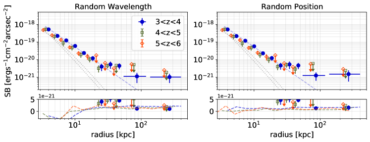
Figure 3: The median Ly$\alpha$ surface brightness profiles of our MXDF LAE sample after subtracting the systematic surface brightness offset. The left and right columns present the two methods for measuring the systematic offset (Section 2.4), by inserting fake objects at the same sky position as the real LAEs but in different wavelength layers (left column), and by inserting fake objects in the same wavelength layers but at different sky positions (right column). The blue dashed lines show the power-law fit. The small panels at the bottom show the systematic offset on a linear $y$-scale. The final radial bin is centered at 270 kpc, but it includes signal out to $\approx$470 kpc. Different colors show different redshift ranges. All the symbols are slightly shifted horizontally for better visualization. We plot the PSFs in the MXDF at 3000Å and 9000Å for comparison (dotted lines).

Figure 3 presents the median Ly$\alpha$ surface brightness profiles around LAEs in different redshift ranges. The left and right panels show the two measurements of the systematic surface brightness offset. The PSFs of the MXDF at 5000Å and 9000Å are also plotted for comparison. For all redshift ranges, the median Ly$\alpha$ surface brightness profiles are clearly more extended than the PSF.

In the left and right columns of Figure 3, we compare the surface brightness profiles correcting from the systematic offset estimated using the two independent methods presented in Section 2.4. These two independent measurements give consistent results. In the following sections we only show the results of the $Random\;Wavelength$ method. However, we verified that the results of $Random\;Position$ or the average of these two methods does not change our conclusions.

As shown by the blue dots in Figure 3, at $3<z<4$, we detect the extended Ly$\alpha$ emission out to hundreds of kpc. Within approximately 20 kpc, the Ly$\alpha$ surface brightness exhibits a gradual decrease. If we consider solely the scattering of Ly$\alpha$ photons from the central galaxy to the CGM, a power-law surface brightness profile with a slope of -2.4 has been predicted (Kakiichi & Dijkstra, 2018). We apply a power-law model to our stacked profile, specifically targeting the inner $\approx$20 kpc while also accounting for the PSF effect. The resulting power-law index, $\mathrm{-2.47\pm 0.11}$ agrees with the theoretical prediction, suggesting a notable influence of the scattering effect within this distance.

At radii larger than 20 kpc, a noticeable flattening trend emerges, which is more plausible within the range of 20 to 50 kpc. Within this radial span, the Ly$\alpha$ surface brightness stays at a level of $\mathrm{4.73\pm 1.95\times\ 10^{-21}\,erg\,s^{-1}\,cm^{-2}\,arcsec^{-2}}$. The detections within the 20–50 kpc range have a slightly above 2$\sigma$ significance, which means we cannot entirely rule out variations attributed to errors. Nevertheless, as demonstrated in Section 3.4, this change of slope in the Ly$\alpha$ surface brightness profile at large radius is consistently observed across different data samples and facilities (e.g. Wisotzki et al., 2018; Lujan Niemeyer et al., 2022b).

The furthest radial bin includes signals as far out as 470 kpc, with its center located approximately at 270 kpc. Within the 50–270 kpc range, we detect a tentative signal, with the combined surface brightness $\mathrm{1.20\pm 0.49\times\ 10^{-21}\,erg\,s^{-1}\,cm^{-2}\,arcsec^{-2}}$. Despite the presence of errors, a comparison with the 20–50 kpc range reveals a break in the Ly$\alpha$ surface brightness at 50–270 kpc, with a drop occurring after approximately 50 kpc.

At higher redshift, we do not detect extended emission at as large distance as at $3<z<4$. We achieve a robust detection within approximately 30 kpc and 15 kpc for LAEs at $4<z<5$ and $5<z<6$, respectively. Comparing the three redshift intervals, we do not detect any obvious evolution of the observed Ly$\alpha$ surface brightness profiles. This agrees with previous works (e.g. Wisotzki et al., 2018). When we compare the Ly$\alpha$ surface brightness profiles at different redshift, we cannot ignore the observational effects. Due to the stronger cosmological surface brightness dimming at higher redshift, lower efficiency of MUSE at the red end and the stronger sky background contamination, the high-redshift LAEs in our sample are more luminous than those at $3<z<4$ (see the second panel of Figure 1). As we will show in Section 3.3, there is a strong correlation between Ly$\alpha$ luminosity of the galaxy and the brightness of the LAH. Therefore, observational incompleteness may complicate the comparison of the Ly$\alpha$ surface brightness profiles at different redshift.

Because we detect the extended Ly$\alpha$ haloes out to hundreds of kpc, the neighboring galaxies within the field of view, if they exist, may contribute to the surface brightness profile and are more likely to do so with increasing distance. In Section 3.2, we mask all nearby LAEs to provide a “cleaner” Ly$\alpha$ surface brightness profile. However, since these neighbors are quite common, and we are not able to distinguish two adjacent neighboring LAHs, we take Figure 3 as the more valuable result, that contains all the averaged environmental information at large distance.

3.2 The influence of the nearby galaxies

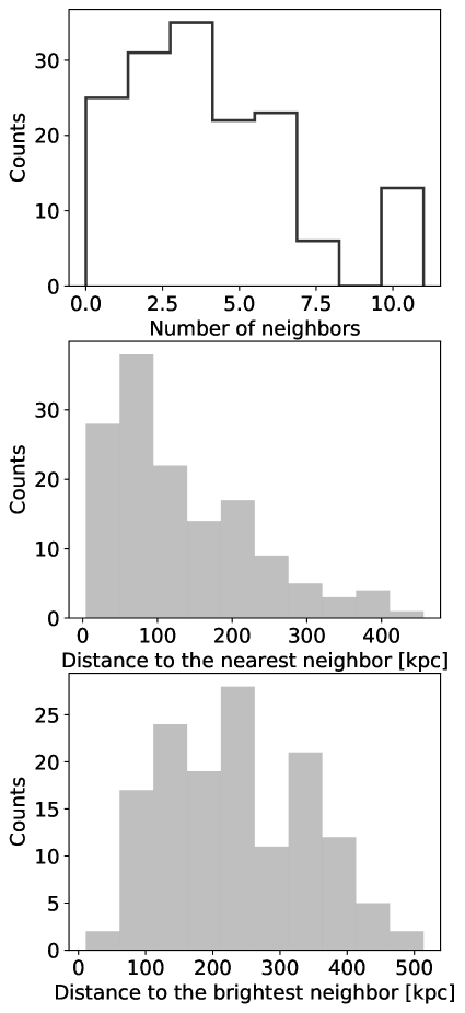
Figure 4: The distribution in the upper panel presents the number of neighbors for each LAE within the NB. The middle panel displays the projected distance to the nearest neighbor. The lower panel displays the projected distance to the brightest neighbor. All three panels are based on the catalogue of the MXDF.

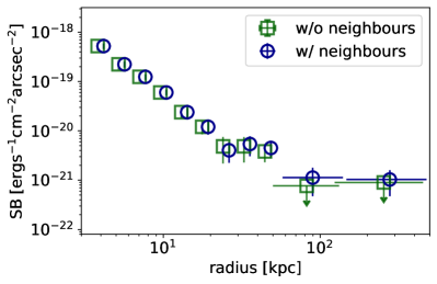
Figure 5: The Ly$\alpha$ surface brightness profiles after masking the neighboring LAEs (green symbols) at $3<z<4$. For comparison, we also plot the profiles before masking the neighboring LAEs (blue symbols). The symbols are slightly shifted horizontally for better visualization.

As we have already mentioned in Section 2.2, since we are detecting the extended Ly$\alpha$ emission at hundreds of kpc, the influence of nearby LAEs (or the nearby LAHs) is inevitable. This is demonstrated by our statistics in Figure 4. In the upper panel of Figure 4, we calculate the number of neighbors for each LAE in the MXDF. Here the neighbor of a LAE is defined as any LAE at the field of view and its Ly$\alpha$ peak wavelength $\pm$ 0.5$\times$FWHM at the wavelength range of the same NB. The LAE and its neighbor(s) are within a projected distance of 1’, but not necessarily physically or gravitationally related. The distribution in Figure 4 is highly observationally-biased, as the sample incompleteness changes with redshift and because neighbors can also exist outside the field of view. Despite this incompleteness, we find that out of 369 LAEs in the MXDF, only 36 LAEs do not have any detected neighbor within the same NB. Although it is not shown in Figure 4, we also take into account the LAEs identified in the MOSAIC, that includes the brighter neighbors at larger distance. After including the MOSAIC LAEs, only 1 out of the 369 LAEs is totally isolated. The number of the neighbors can exceed 30.

In the middle panel of Figure 4, we present the distance of a MXDF LAE to its nearest neighbor. In the lower panel of Figure 4, we present the distance of a MXDF LAE to the neighbor with the highest Ly$\alpha$ luminosity. The median distance of a LAE to its nearest neighbor is 110 kpc, the 10th and 90th percentiles are 29 and 274 kpc, respectively. The median distance to the brightest neighbor is 226 kpc, the 10th and 90th percentiles are 97 and 377 kpc, respectively. In this case, at the scale of hundreds of kpc, the overlap of the LAHs cannot be ignored. Compared to previous work, this LAH-overlapping problem is more evident for us, because our extremely deep observations identify lots of faint LAEs that could not be detected in previous observations. In fact, the previous work, restricted by observational depth or spatial resolution, cannot remove the effect of the neighboring LAEs to get a “cleaner” radial profile. In other words, the previous observations with shorter integration time or lower spatial resolution already included lots of faint neighbors in their Ly$\alpha$ surface brightness profiles.

We provide another measurement of the Ly$\alpha$ surface brightness profile by excluding the nearby LAEs. In each NB, except the target LAE, we mask all the nearby galaxies based on the segmentation images given by Bacon et al. (2023). Then we compute the median profiles following the same procedures as in Section 2.3. This operation only removes the bright area of the nearby LAHs, because we are not able to decompose each galaxy from its LAH. The final surface brightness profile may still contain the diffuse content of the nearby LAHs.

The median Ly$\alpha$ surface brightness profile after masking the neighboring LAEs is shown by the green dots in Figure 5. For comparison, we also show the Ly$\alpha$ surface brightness profile before masking the neighbors (blue dots in Figure 5, same as Figure 3). Within the inner 50 kpc, the two profiles are very similar, though there are inconspicuous differences at 20-50 kpc. Beyond 50 kpc we do not get a robust detection after masking the neighbors. The upper limits in the last two radial bins further show the break of the Ly$\alpha$ surface brightness profile at $\approx$ 50 kpc. Limited by the radial sampling and the S/N, we are not able to provide better constraints on this break, in particular its exact distance. However, the downward trend of the profile is quite robust. After stacking the outer two radial bins, we provide a 2-sigma upper limit of Ly$\alpha$ surface brightness at 50-270 kpc of $\mathrm{0.93\times\ 10^{-21}\,erg\,s^{-1}\,cm^{-2}\,arcsec^{-2}}$, about more than half an order-of-magnitude lower than the surface brightness at 20-50 kpc.

The potential flattening of the Ly$\alpha$ surface brightness profile beyond 20 kpc is intriguing. This observation suggests a change in the dominant mechanism(s) responsible for producing Ly$\alpha$ photons at varying distances. Moreover, the possible break at around 50 kpc likely indicates that the mechanisms governing the production and propagation of Ly$\alpha$ photons at smaller radii become less influential at larger distances.

3.3 The LAHs of bright and faint LAEs

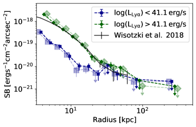
Figure 6: The Ly$\alpha$ surface brightness profiles at $3<z<4$. We split the LAE sample into two subsamples based on $\mathrm{L_{Ly\alpha}}$. The profiles before masking the neighboring LAEs are shown by small symbols. The profiles after masking are shown by light-colored large symbols. For comparison, we also plot the result of Wisotzki et al. (2018). The symbols are slightly shifted horizontally for better visualization.

To study the possible correlations between Ly$\alpha$ surface brightness profiles and LAE properties, we divide the LAE sample at $3<z<4$ into two subsamples based on the median Ly$\alpha$ luminosity $\mathrm{L_{Ly\alpha}}$. The corresponding Ly$\alpha$ surface brightness profiles are shown in Figure 6. The green and blue dots present the high- and low-$\mathrm{L_{Ly\alpha}}$ subsamples, respectively. For each subsample, we show the profiles before and after masking the neighboring galaxies.

For all subsamples, the Ly$\alpha$ surface brightness profiles decrease within approximately 20 kpc. The Ly$\alpha$ profiles of high- and low-$\mathrm{L_{Ly\alpha}}$ LAEs have similar slopes, but the normalisation is $\approx$1-dex fainter for the low-$\mathrm{L_{Ly\alpha}}$ subsample. This suggests that the production of Ly$\alpha$ photons in the central galaxies plays an important role in boosting the LAHs within $\approx$20 kpc, and that the mechanisms that produce and propagate the Ly$\alpha$ photons outward may scale with $\mathrm{L_{Ly\alpha}}$.

At larger radii ($\gtrsim$20 kpc), the two radial profiles show evidence of flattening, despite the large errors (or upper limits). The flattening trend appears for both subsamples, but the change occurs at a shorter distance for the low-$\mathrm{L_{Ly\alpha}}$ subsample.

As we have discussed in Section 3.2, nearby LAEs are contributors to the LAHs at distances larger than 50 kpc. The trend is not very clear for the two subsamples, because the S/N is low. Still, the measured values (or upper limits) before masking the neighboring galaxies are slightly higher than those after masking the neighboring galaxies. Nonetheless, the contribution from neighboring galaxies may not be the key reason for the flattening of the profiles at 20-50 kpc, which has already been demonstrated by Section 3.2 and Figure 5.

The Ly$\alpha$ surface brightness profile of higher-$\mathrm{L_{Ly\alpha}}$ LAEs agrees with Wisotzki et al. (2018). The sample of Wisotzki et al. (2018) is built from brighter LAEs in the UDF-10 and MOSAIC fields. The good agreement between Wisotzki et al. (2018) and our high-$\mathrm{L_{Ly\alpha}}$ profile further demonstrates the robustness of our measurement. Similar to our work here, Wisotzki et al. (2018) split their LAE sample by $\mathrm{L_{Ly\alpha}}$. They also reach a similar conclusion that the radial profiles follow the same trend but with different normalisations of the surface brightness.

3.4 Comparison of different datasets

We have shown the median Ly$\alpha$ surface brightness profiles of LAEs at $3<z<4$ out to $\approx$270 kpc using the MXDF data. In this section, we firstly try to detect the Ly$\alpha$ signal at larger distance. The MOSAIC is a good supplement to the MXDF, with $\approx$9 times larger sky coverage but at the expense of 10-14 times shorter integration time. We would like to use MOSAIC to constrain the median Ly$\alpha$ surface brightness as far as 1000 kpc. We present the radial profile in Figure 7. We do not achieve a robust detection at the distance of 60-1000 kpc. Instead, we provide a 2-sigma upper limit of $\mathrm{2.82\times\ 10^{-21}\,erg\,s^{-1}\,cm^{-2}\,arcsec^{-2}}$.

In Figure 7 we compare with the Ly$\alpha$ surface brightness profiles of Wisotzki et al. (2018). The profile of MOSAIC agrees well with Wisotzki et al. (2018) within approximately 60 kpc. The median Ly$\alpha$ profile of MXDF is about 0.5 dex fainter than that of the MOSAIC and Wisotzki et al. (2018). Considering that the shallower observation of the MOSAIC can only identify the bright LAEs (Figure 1), this comparison of Ly$\alpha$ surface brightness profiles in the MOSAIC and the MXDF reflects again the trend with $\mathrm{L_{Ly\alpha}}$ (see Figure 6).

We also show the observational result of the Hobby-Eberly Telescope Dark Energy Experiment (HETDEX, Gebhardt et al., 2021). The HETDEX Ly$\alpha$ surface brightness profile around LAEs at $z\approx 2.5$ is provided by Lujan Niemeyer et al. (2022b), and shown by yellow dots in Figure 7. The Ly$\alpha$ surface brightness profile is scaled by $(1+z)^{4}$. Our observation and HETDEX have different PSF size, spatial resolution and observational strategy. HETDEX performs shallow observations over a large sky area, while our MXDF and MOSAIC concentrate on small sky areas with extremely deep exposures. The LAE sample of Lujan Niemeyer et al. (2022b) is 1 order-of-magnitude brighter than our sample. Their typical $\mathrm{L_{Ly\alpha}}$ is $\mathrm{10^{42.8}erg\,s^{-1}}$. For comparison, the median $\mathrm{L_{Ly\alpha}}$ of the MXDF and MOSAIC sample at $3<z<4$ are $\mathrm{L_{Ly\alpha,MXDF}\approx 10^{41.1}erg\,s^{-1}}$ and $\mathrm{L_{Ly\alpha,MOSAIC}\approx 10^{41.5}erg\,s^{-1}}$ respectively. In Figure 7, the profiles are strongly influenced by the different PSF. Lujan Niemeyer et al. (2022b) tried to re-scale the profile of Wisotzki et al. (2018) to their PSF size and LAE luminosity, and get very good agreement.

Despite the different luminosities, observational facilities and noise levels, the Ly$\alpha$ surface brightness profiles of the MXDF, MOSAIC, and Lujan Niemeyer et al. (2022b) show similar patterns. Among these datasets, the MXDF obviously achieves a deeper detection limit. Therefore, here we take the radial profile of the MXDF as an example. At small distances, the profile shows a power law decrease. The normalisation of the profile depends strongly on $\mathrm{L_{Ly\alpha}}$. Then the profile likely reaches a plateau. The transition between the decrease and plateau appears at $\approx$20 kpc for MXDF. The transition distance increases with higher $\mathrm{L_{Ly\alpha}}$. Beyond the plateau ($\approx$50 kpc for MXDF), the profile likely drops to a very low surface brightness level, and becomes dominated by neighboring galaxies (Section 3.2). The distance of this break also increases with $\mathrm{L_{Ly\alpha}}$.

Note that a similar trend is also observed in the Ly$\alpha$ surface brightness profile of quasars at $2<z<4$, though the physical mechanisms in behind may be different. Several works find that the Ly$\alpha$ surface brightness profile within the distance of approximately 100 kpc to the quasar decrease by a power with power law index of approximately -1.8 (e.g. Borisova et al., 2016; Cai et al., 2019). According to Lin et al. (2022), the profile within 1 cMpc decreases by a similar power law. At larger radii (1-100 cMpc), the profile shows a flatter slope but with large variation, which can be well explained by a two halo-term of the clustered Ly$\alpha$ sources.

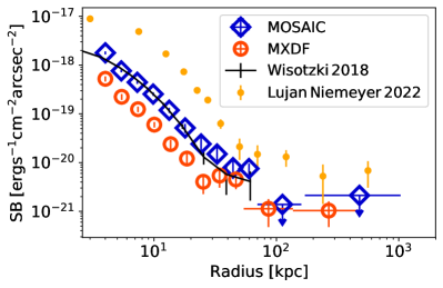
Figure 7: The Ly$\alpha$ surface brightness profiles of LAEs at $3<z<4$ in the MOSAIC field (blue symbols) and in the MXDF field (red symbols). Both profiles include nearby LAEs. For comparison, we also plot the result of Wisotzki et al. (2018) and Lujan Niemeyer et al. (2022b). The Lujan Niemeyer et al. (2022b) profile is scaled by $(1+z)^{4}$.

4 Discussion

4.1 Physical origins of the LAHs

While the existence of LAHs around star-forming galaxies at $2<z<6$ has been confirmed by previous works (e.g. Steidel et al., 2011; Matsuda et al., 2012; Momose et al., 2014; Wisotzki et al., 2016, 2018; Leclercq et al., 2017; Kusakabe et al., 2022), there is no consensus yet on the dominant physical mechanism giving rise to the LAHs. Several physical origins are on the list (e.g. Momose et al., 2016; Ouchi et al., 2020), including the resonant scattering of Ly$\alpha$ photons produced by recombination of gas photoionized by star formation or an AGN (in the central galaxy and also in unresolved satellites), the collisional excitation and recombination in cooling gas flowing into a galaxy, as well as the fluorescent emission from the UV background. The dominant origin of the Ly$\alpha$ photons may change with the distance to the galaxies (e.g. Lake et al., 2015; Mitchell et al., 2021; Byrohl et al., 2021).

In this work, we detect Ly$\alpha$ emission around LAEs extending out to $\approx$270 kpc by median-stacking a representative sample of LAEs (Figure 3), re-demonstrating that LAHs are a common property of LAEs. Our measurement provides the typical Ly$\alpha$ surface brightness profile around the LAE with median Ly$\alpha$ luminosity $\mathrm{\approx 10^{41.1}erg\,s^{-1}}$. In this section, we will discuss the dominant physical origin of the Ly$\alpha$ photons at different radial ranges.

Before discussing the physics dominating at different distances, we firstly clarify the difference between the extent of the LAHs and the size of dark matter haloes. Following the method of Leclercq et al. (2017), we estimate the virial radius based on the $r_{vir}$ - UV magnitude relation predicted by the semi-analytic model of Garel et al. (2015). The typical virial radius $r_{vir}$ of the MXDF LAEs is approximately 20 kpc. The estimation of $r_{vir}$ is always model-dependent and we expect a large amount of scatter. Our detection of extended Ly$\alpha$ emission out to $\approx$270 kpc implies that the Ly$\alpha$ emission can extend to $\gtrsim$10 times larger radii than $r_{vir}$.

4.1.1 $\mathrm{r\lesssim 20\leavevmode\nobreak\ kpc}$

The production of Ly$\alpha$ photons in the inner region of the LAH is closely related to the “central engine”, e.g., the star formation in the galaxy. The Ly$\alpha$ photons are produced by recombination in the star-forming regions of the host galaxy, part of them succeed in escaping the dusty ISM. The existence of outflows may help the escape of Ly$\alpha$ photons. These escaped Ly$\alpha$ photons can be scattered by the neutral hydrogen in the CGM and produce the observed LAH. Spectroscopic observations find that the majority of Ly$\alpha$ lines are red-shifted with respect to the systemic redshift and have red-asymmetric profiles, which is interpreted as a signature of galactic outflows (e.g. Verhamme et al., 2006; Schaerer et al., 2011; Dijkstra & Kramer, 2012; Chang et al., 2022). Such a model of Ly$\alpha$ scattering through outflowing media has been successful in reproducing the observed Ly$\alpha$ spectral and surface brightness profiles (e.g. Yang et al., 2016; Song et al., 2020; Li et al., 2022).

In our analysis, within the central $\approx$20 kpc ($r_{vir}$), the Ly$\alpha$ surface brightness profile drops down as a power law with increasing radius (Figure 3). As is shown in Figure 6, dividing the sample into high-$\mathrm{L_{Ly\alpha}}$ and low-$\mathrm{L_{Ly\alpha}}$ subsamples results in similarly shaped Ly$\alpha$ surface brightness profiles, but the normalisation increases with $\mathrm{L_{Ly\alpha}}$. This is also seen in Figure 7 by comparing datasets spanning a larger range of $\mathrm{L_{Ly\alpha}}$. If we assume that the Ly$\alpha$ photons within this radius are primarily produced by star formation, the similar slopes of the high-$\mathrm{L_{Ly\alpha}}$ and low-$\mathrm{L_{Ly\alpha}}$ subsamples suggest that the production and propagation mechanism of the Ly$\alpha$ photons in the inner CGM are similar for LAEs with different $\mathrm{L_{Ly\alpha}}$.

4.1.2 $\mathrm{20\lesssim r\lesssim 270\leavevmode\nobreak\ kpc}$

At this distance of $\mathrm{20\lesssim r\lesssim 270\leavevmode\nobreak\ kpc}$, the Ly$\alpha$ surface brightness profile exhibits a trend of flattening (Figure 3), despite the variation of errors. This trend is more robustly observed at 20-50 kpc ($\approx$1-3 $r_{vir}$). At this radial span, the Ly$\alpha$ surface brightness profile only exhibits marginal inconsistency after masking the nearby LAEs (Figure 5). As is shown in Figure 4, neighboring LAEs start to emerge at tens of kpc, but the majority is at hundreds of kpc. These findings suggest that the flattening trend observed cannot be solely attributed to the presence of nearby detected LAEs. The interpretation of the Ly$\alpha$ surface brightness profile at this distance (20-50 kpc) is complicated, because multiple factors are at play. At this distance, the neighbors start to have an effect, and the “central engine” begins to lose its dominance. The flattening of the Ly$\alpha$ profile likely indicates a change in the dominant power source, which can be explained as signs of cooling radiation or undetected satellites, or a mixture of all (e.g. Haiman et al., 2000; Rosdahl & Blaizot, 2012; Mitchell et al., 2021). The Ly$\alpha$ emission at large distance to the central galaxy can also be explained as the fluorescence emission from gas illuminated by the UV background (e.g. Cantalupo et al., 2005; Mas-Ribas & Dijkstra, 2016). For example, Gallego et al. (2021) use the Ly$\alpha$ emission at large distance to constrain the photoionization rate of hydrogen and the covering fraction of Lyman limit systems, based on the assumption that all the Ly$\alpha$ emission at large distances originates from Ly$\alpha$ fluorescence in optically thick H I clouds.

Compared to 20-50 kpc, the Ly$\alpha$ surface brightness profile is likely to drop at approximately 50 kpc, and then stays at a lower surface brightness level out to 270 kpc (Figure 3). This potential break at approximately 50 kpc is clearer after we remove the nearby LAEs. In Figure 5, after masking the nearby LAEs within the same NB, the Ly$\alpha$ emission at 50-270 kpc is below the detection limit. The comparison of the two profiles in Figure 5 thus shows that bright nearby LAHs make a major contribution to the observed Ly$\alpha$ surface brightness profile at 50-270 kpc ($\gtrsim 3r_{vir}$).

In the simulations of Mitchell et al. (2021), the LAHs at $3<z<4$ at tens of kpc are mainly powered by satellite galaxies. The neighbors defined in this work (Section 3.2) are not necessarily bounded within the gravitational potential of a more massive galaxy. The clustering analysis of Herrero Alonso et al. (2023) suggests that only $\lesssim$10% of the MXDF LAEs (same as our LAE sample) are satellites. Therefore, in our case, the neighbors that contribute to the LAHs at 50-270 kpc are mostly bright central galaxies instead of satellites. Byrohl et al. (2021) study a similar case. They apply Monte Carlo radiative transfer of Ly$\alpha$ to TNG50 cosmological magnetohydrodynamical simulations. Their simulations find that most Ly$\alpha$ photons at large radii originate from nearby bright haloes and are then scattered in the CGM of the target halo and also in the IGM. In our work, taking advantage of deep exposures and high spatial resolution, we directly observe the LAHs being enhanced by nearby bright LAEs (Figure 6).

Therefore, at radii of 50-270 kpc, we can confirm that the star formation in nearby bright LAEs provides a major contribution to the extended Ly$\alpha$ emission. The contribution of other Ly$\alpha$ emission mechanisms at these radii, including cooling radiation, flourescence, and satellite galaxies, cannot be robustly measured. Instead, we provide an upper limit on the total of these mechanisms (Section 3.2).

The potential break observed in the Ly$\alpha$ surface brightness profile at approximately 50 kpc is intriguing. Limited by the S/N, we cannot rule out the possibility of error variations. Here we provide a few speculative considerations. It seems to indicate a quick change in the powering mechanism of the LAH or physical state of the CGM at this distance. This may suggests a typical clustering pattern of satellites, or enhancement of the Ly$\alpha$ flux due to collisional excitation of gas inflows at $\mathrm{20\lesssim r\lesssim 50\leavevmode\nobreak\ kpc}$. Another possibility is that the neutral hydrogen density decreases at approximately 50 kpc. According to the simulations of Mitchell et al. (2021), the hydrogen number density shows a hint of decrease with radius, but their simulations stops at 1 $r_{vir}$. The gas state and physical processes at large distance to the galaxy (around 3 $r_{vir}$ in our case) is not very clear. To further address this question, we conduct detailed simulations as will be described in Guo et al. in preparation.

4.2 The Ly$\alpha$ surface brightness profile as a cross-correlation function

Intensity mapping of the cumulative Ly$\alpha$ and other emission lines (e.g., H I, CO) has been proposed as a a powerful tool for understanding the line emissivity and the large-scale matter distribution in the Universe (e.g. Bernal & Kovetz, 2022). In particular, by stacking the cross-correlation functions (CCFs) between the source redshift catalogue and maps expected to include Ly$\alpha$ emission from the same sources, efforts have been made to constrain the integrated Ly$\alpha$ emission over large cosmological volumes (e.g. Croft et al., 2016, 2018; Kakuma et al., 2021; Kikuchihara et al., 2022; Lin et al., 2022). Based on the Sloan Digital Sky Survey (DR12) spectra, Croft et al. (2016, 2018) measure the cross-correlation between quasar positions and Ly$\alpha$ emission imprinted in the residual spectra of luminous red galaxies. They detect positive signal of extended Ly$\alpha$ emission around quasars on scales as far as 15 cMpc. This measurement is renewed by Lin et al. (2022), using DR16 of the Sloan Digital Sky Survey. The extended Ly$\alpha$ emission around normal galaxies is orders-of-magnitude fainter than the quasars and thus more difficult to detect. Recently, positive detections of the Ly$\alpha$-LAE CCF as far as $\approx$1 cMpc have been obtained by stacking deep NB images around bright LAEs (Kakuma et al., 2021; Kikuchihara et al., 2022).

In the 2 dimensional case, the CCF between Ly$\alpha$ emission intensity and the position of a given LAE mathematically equals the Ly$\alpha$ surface brightness at different radii (e.g. Kakuma et al., 2021). Restricted by the sky area of the MXDF and MOSAIC, our observations are not ideal for mapping the extended emission at a scale of several cMpc, but the extremely deep exposure and good spatial resolution provide a unique experiment that identifies very faint galaxies and foreground contaminators. This could be a good supplement to Ly$\alpha$ intensity mapping experiments. Our work is more efficient in removing line and continuum contaminators. Our dedicated pseudo-NBs include all the potential signal but not extra noise. More importantly, we quantify the contribution of the faint LAEs that are not detected in previous works, and anonymously contribute to their Ly$\alpha$ CCFs.

Our precise and reliable measurement of the Ly$\alpha$ surface brightness profile will be helpful for the design of future intensity mapping experiments, which usually have lower spatial resolution and perform much shallower observations. It would also be very meaningful to compare our CCFs with cosmological simulations.

5 Summary

Thanks to the extremely deep MUSE observations of the Hubble Ultra Deep Field, we unveil the typical Ly$\alpha$ surface brightness profile around LAEs down to unprecedented depth and distance. Our major results are summarized below.

Based on the MXDF data, we present the median Ly$\alpha$ surface brightness profiles of LAEs with Ly$\alpha$ luminosity $\mathrm{\approx 10^{41.1}erg\,s^{-1}}$ at $3<z<4$. After carefully correcting for the systematic surface brightness offsets of the MUSE datacube, we detect extended Ly$\alpha$ emission out to 270 kpc. The Ly$\alpha$ surface brightness profile decreases as a power law within a radius of 20 kpc, followed by a flattened profile at 20-50 kpc, and a potential drop to a lower level at 50-270 kpc. We observe a possible break in the Ly$\alpha$ profile at a radius of approximately 50 kpc.

We find that the nearby LAEs make a major contribution to the Ly$\alpha$ surface brightness profile at 50-270 kpc, at the level of $\mathrm{1.20\pm 0.49\times\ 10^{-21}\,erg\,s^{-1}\,cm^{-2}\,arcsec^{-2}}$. In addition, we provide an upper limit on the contribution of other physical mechanisms to the profile at this distance, which is estimated to be $\mathrm{0.93\times\ 10^{-21}\,erg\,s^{-1}\,cm^{-2}\,arcsec^{-2}}$.

We divide our LAE sample in subsamples by $\mathrm{L_{Ly\alpha}}$. Within approximately 20 kpc, the high-$\mathrm{L_{Ly\alpha}}$ sample exhibits a higher Ly$\alpha$ surface brightness profile, but the profiles of different subsamples have similar slopes. This indicates that star formation in the central galaxy may dominate the Ly$\alpha$ surface brightness at small distance. The production and propagation of Ly$\alpha$ photons likely follows similar mechanisms in different subsamples.

We attempt to detect the extended Ly$\alpha$ emission at larger radii using MOSAIC. We are not able to provide a robust detection from 60 kpc to 1 Mpc , but provide an upper limit of $\mathrm{2.82\times\ 10^{-21}\,erg\,s^{-1}\,cm^{-2}\,arcsec^{-2}}$.

Although this work mainly focuses on the LAHs at $3<z<4$, we find that there is no significant evolution in the observed Ly$\alpha$ surface brightness profiles when we compare with $4<z<5$ and $5<z<6$.

Our results support a scenario in which star formation in the central galaxy dominates the LAHs at small radii (within 20 kpc), while Ly$\alpha$ photons from nearby galaxies dominate the Ly$\alpha$ surface brightness at large radii (50-270 kpc). The Ly$\alpha$ surface brightness profile at the distance range of 20-50 kpc is more difficult to interpret. Deeper observations of the Ly$\alpha$ line profiles and further simulations are needed.