Energy-optimal Timetable Design for Sustainable Metro Railway Networks

Abstract

We present our collaboration with Thales Canada Inc, the largest provider of communication-based train control (CBTC) systems worldwide. We study the problem of designing energy-optimal timetables in metro railway networks operated by CBTC to minimize the effective energy consumption of the network, which corresponds to simultaneously minimizing total energy consumed by all the trains and maximizing the transfer of regenerative braking energy from suitable braking trains to accelerating trains. We propose a novel data-driven linear programming model that minimizes the total effective energy consumption in a metro railway network, capable of computing the optimal timetable in real-time, even for some of the largest CBTC systems in the world. In contrast with existing works, which are either NP-hard or involve multiple stages requiring extensive simulation, our model is a single linear programming model capable of computing the energy-optimal timetable subject to the constraints present in the railway network. Furthermore, our model can predict the total energy consumption of the network without requiring time-consuming simulations, making it suitable for widespread use in managerial settings. We apply our model to Shanghai Railway Network’s Metro Line 8—one of the largest and busiest railway services in the world—and empirically demonstrate that our model computes energy-optimal timetables for thousands of active trains spanning an entire service period of one day in real-time (solution time less than one second on a standard desktop), achieving energy savings between approximately 20.93% and 28.68%. The model’s computational efficiency negates the need for time-intensive simulations traditionally used for timetable optimization, thereby streamlining the planning process. It can also be generalized and deployed across any CBTC system, making it a broadly applicable tool for sustainable timetable planning. Given these compelling advantages, our model is in the process of being integrated into Thales Canada Inc’s industrial timetable compiler.

Keywords.

Metro railway networks, Sustainability, Train scheduling, Energy-efficiency, Communication-based train control

Introduction

Background.

As projections indicate that the global urban population is poised to increase from 54% to 66% by the year 2050 [27], the urgency to enhance both the efficiency and sustainability of urban transit systems is escalating. Faced with an estimated influx of 2.5 billion urban inhabitants, there is an impending imperative to restructure existing transportation infrastructure. Rail transit, lauded for its substantial passenger-carrying capacity and safety metrics [1], is strategically positioned to play a crucial role in this infrastructural transformation. Notably, Communication-Based Train Control Systems (CBTC) have a significant impact on the effective functioning of these rail networks [23]. Utilized by some of the world’s busiest metros, CBTC systems offer high-resolution train location determination and continuous data communications. These capabilities significantly improve both safety and efficiency and allow for dynamic adjustments in operational schedules, offering solutions to traffic congestion and fluctuating demand. Thanks to technological advancements like built-in redundancy, modern CBTC systems are also more reliable and easier to maintain. CBTC systems are particularly conducive to developing sustainable and energy-efficient operations, owing to functionalities like the ability to implement automatic driving strategies and the precise implementation of a provided railway timetable [13]. In light of these multi-dimensional advantages, the integration of real-time, energy-efficient timetable optimization within CBTC-enabled railway networks emerges as a cornerstone strategy. This strategic integration not only amplifies operational efficiency and adaptability but also contributes to achieving broader environmental sustainability goals. Hence, it aligns perfectly with the imperatives of modern urban transport, which must be both highly efficient and demonstrably sustainable to meet the complex demands of an increasingly urbanized global landscape.

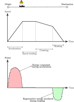
Figure 1: This figure graphically illustrates a train’s energy consumption and regeneration cycle in CBTC systems. When a train makes a trip from the origin platform to the destination platform, it transitions through four phases - acceleration, speed holding, coasting, and braking, as shown in the speed vs. time graph at the top. The acceleration phase requires the most amount of energy energy, as denoted by the red-shaded area in the power vs. time graph at the bottom. In contrast, the speed holding and coasting phases entail minimal to zero energy usage. Notably, during the braking phase, the train produces regenerative braking energy, represented by the green-shaded area in the power vs. time graph. With appropriate scheduling, this energy can be strategically transferred to nearby accelerating trains.

Motivation.

Electricity is the energy source for trains in all modern metro railway networks that utilize CBTC systems. When trains make trips from origin platforms to destination platforms, their speed profile consists of four phases: acceleration, speed holding, coasting, and braking [12], as shown qualitatively in Figure 1. Among these phases, trains consume most of their energy during acceleration. Conversely, when trains brake, the electric motors that make the trains move during the acceleration phase work in reverse, becoming generators. They convert the trains’ kinetic energy into electrical energy, referred to as regenerative braking energy. CBTC systems are capable of implementing a given timetable precisely, which allows for the transfer of this regenerative energy from braking trains to nearby accelerating trains. For empirical context, the New York City transit railway system, which consumes more than 1,600 GWh of electricity per year, has had all of its trains installed since 2018 capable of producing and transferring regenerative braking energy. Under favorable conditions, the regenerative energy produced can account for up to 50% of the energy consumed [22].

Energy-optimal timetable.

The conceptualization and implementation of an energy-optimal timetable offer avenues for substantial energy conservation, obviating the need for infrastructural alterations within CBTC-enabled railway systems. Formally, a railway timetable is a data structure, containing both the arrival and departure times of each train at every platform visited during a designated service period—typically spanning 18 to 24 hours in most operational networks. The core objective of an energy-optimal timetable is to strategically design these temporal decision variables to minimize the network’s effective energy consumption, which equals the total energy consumption for all trains during their accelerating phases minus the total regenerative braking energy successfully transferred to the accelerating trains from eligible braking counterparts.

Related work.

Recent years have seen noteworthy contributions to energy-efficient railway timetable computation. For instance, [24] proposes a mixed integer programming (MIP) model limited to single train-lines with successful application on Madrid’s Line 3. The work in [5] presents a more tractable MIP model for optimizing regenerative energy transfer between suitable train pairs, applied to the Dockland Light Railway, but does not directly address the actual energy savings. The work in [17] employs a genetic algorithm to calculate energy-efficient timetables. Their approach seeks to maximize the use of regenerative energy while minimizing the tractive energy of trains. Similarly, [16] introduces a nonlinear integer programming model that utilizes simulated annealing. The model [32] proposes a non-dominated sorting genetic algorithm for a biobjective timetable optimization model, uniquely incorporating energy allocation and passenger assignment. Continuing in the same vein, Wang and Goverde have conducted studies on multi-train trajectory optimization: their method treats the problem as a multiple-phase optimal control problem, solved by a pseudospectral method [28]. Furthermore, they introduce an innovative approach to energy-efficient timetabling that adjusts the running time allocation of given timetables using train trajectory optimization [29].

From an industry implementation standpoint, the two-stage linear optimization model [6] is, to our knowledge, the sole optimization model incorporated into an industrial timetable compiler operated by CBTC. This model presents a two-step linear optimization model for developing an energy-efficient railway timetable. The first stage minimizes total energy consumption for all trains, considering the railway network’s constraints. The second stage fixes the trains’ trip times to those computed in the first stage and maximizes the transfer of regenerative braking energy between suitable train pairs. However, this model has some limitations. First, although the optimization problems in the first and second stages are solved quickly (in minutes), transitioning between stages requires a time-consuming (in hours) intermediate simulation process, significantly extending the end-to-end runtime. Second, the model in [6] does not directly model the network’s actual energy consumption, rather it employs proxy objective functions, the optimization of which might lead to an energy-efficient timetable indirectly. This roundabout approach necessitates extensive physics-based simulations a posteriori to predict the actual reduction in energy consumption. This could limit its applicability in managerial settings, where the model’s perceived utility is directly tied to its ability to predict energy consumption levels. Finally, the model requires the precise locations of energy consumption peaks, which are often unavailable, to formulate the optimization problem for the second stage.

Contribution.

We develop a novel single-stage linear optimization model to construct energy-optimal timetables for all the trains in a CBTC-enabled metro railway network for an entire service period. We directly model the total energy consumption, total savings of regenerative energy, and the interaction between regenerative and consumed energy using a data-driven approach. Unlike existing works, our model can predict total energy consumption without requiring time-consuming simulations, making it suitable for widespread use in managerial settings. We also model the transfer of regenerative energy through a set of linear constraints, whereas the existing works use nonconvex constraints. We empirically demonstrate that our model performs extremely well when applied to Metro Line 8 of the Shanghai Railway network, which is one of the busiest railway services in the world in terms of ridership and number of trains. We deploy a warm-started parallel barrier algorithm to solve our linear optimization model, which computes energy-optimal timetables for a full service period of one day with thousands of active trains in real-time (solution time is less than a second on a standard desktop). The optimal timetables exhibit a significant reduction in effective energy consumption in comparison with existing real-world timetables, ranging between approximately 20.93% to 28.68%. Our proposed model offers transformative benefits for managerial decision-making within metro railway networks employing CBTC systems. It not only significantly speeds up the planning process by sidestepping traditional, time-intensive simulations but is also versatile enough for generalized application across any CBTC system. Recognizing these advantages, our model is in the process of being implemented into Thales Canada Inc’s industrial timetable compiler.

Organization

The paper is organized as follows. In Section 2, we present the notation and notions used in this paper. Then in Section 3, we discuss the constraints that are necessary for proper functioning of a metro railway network. In Section 4, we present how we model the objective of effective energy consumption. The final optimization model is presented in Section 5. We present our numerical experiments applied to the Shanghai Railway Network in Section 6. We describe the architectural framework for industrial integration of our optimization model in Section 7.

Notation and notions

All the sets described in this paper are strictly ordered and finite unless otherwise specified. The cardinality and the $i$-th element of such a set $S$ are denoted by $|S|$ and $S(i)$, respectively.

Table 1: List of symbols in the order they appear in the paper.

Symbol	Description
$\mathcal{N}$	The set of all platforms in a railway network
$\mathcal{A}$	The set of all tracks
$\mathcal{T}$	The set of all trains
$\mathcal{N}^{t}$	The set of all platforms visited by a train $t$ in chronological order
$\mathcal{A}^{t}$	The set of all tracks visited by a train $t$ in chronological order
$a_{i}^{t}$	The arrival time of train $t$ at platform $i$ (decision variable)
$d_{i}^{t}$	The departure time of train $t$ from platform $i$ (decision variable)
$[\underline{\tau}_{ij}^{t},\overline{\tau}_{ij}^{t}]$	The track-based trip time window for train $t$ from platform $i$ to platform $j$
$\varphi$	The set of all crossing-overs in the network
$\mathcal{B}_{ij}$	The set of all train pairs involved in turn-around events on crossing-over $(i,j)$
$[\underline{\kappa}_{ij}^{tt^{\prime}},\overline{\kappa}_{ij}^{tt^{\prime}}]$	The trip time window for train $t$ on the crossing-over $(i,j)$
$[\underline{\delta}_{i}^{t},\overline{\delta}_{i}^{t}]$	The dwell time window for train $t$ at platform $i$
$\chi$	The set of all platform pairs situated at the same interchange stations
$\mathcal{C}_{ij}$	The set of connecting train pairs for a platform pair $(i,j)\in\chi$
$[\underline{\chi}_{ij}^{tt^{\prime}},\overline{\chi}_{ij}^{tt^{\prime}}]$	The connection window between train $t$ at platform $i$ and and train $t^{\prime}$ at platform $j$
$\mathcal{H}_{ij}$	The set of train-pairs who move along that track $(i,j)$
$h_{i}^{tt^{\prime}}$	The headway time between train $t$ and $t^{\prime}$ at or from platform $i$
$[\underline{\tau}_{\mathcal{P}}^{t},\overline{\tau}_{\mathcal{P}}^{t}]$	The total travel time window for train $t$ to traverse its train path
$E_{i,j,t}^{\textrm{con,tr}}$	Energy consumed by train $t$ during acceleration while going from platform $i$ to platform $j$
$E_{i,j,t,t^{\prime}}^{\textrm{con,cr}}$	Energy consumed by train $t$ during acceleration while traversing the crossing-over $(i,j)\in\varphi$
$\Omega$	The set of all platform pairs that are feasible for regenerative energy transfer
$\mathcal{T}_{i}$	The set of all trains which arrive at, dwell and then depart from platform $i$
$\overset{\rightharpoonup}{t}$	Temporally close train to the right of train $t$
$\overset{\leftharpoonup}{t}$	Temporally close train to the left of train $t$
$\tilde{t}$	Temporally closes train to train $t$
$\mathcal{E}$	The set of all synchronization processes between suitable train pairs
$\overset{\rightharpoonup}{\mathcal{E}}$	A subset of $\mathcal{E}$ containing elements of the form $(i,j,t,\overset{\rightharpoonup}{t})$
$\overset{\leftharpoonup}{\mathcal{E}}$	A subset of $\mathcal{E}$ containing elements of the form $(i,j,t,\overset{\leftharpoonup}{t})$
$E_{i,j,t,\overset{\rightharpoonup}{t}}^{\textrm{reg}}$	Regenerative energy transferred to accelerating train $t$ on platform $i$ from braking train $\overset{\rightharpoonup}{t}$ on platform $j$
$\sigma_{ij}^{t\overset{\rightharpoonup}{t}}$	Overlapping time between the effective accelerating phase of train $t$ on platform $i$ and the effective braking
	phase of train $\overset{\rightharpoonup}{t}$ on platform $j$
$E_{i,j,t,\overset{\leftharpoonup}{t}}^{\textrm{reg}}$	Regenerative energy transferred to accelerating train $\overset{\leftharpoonup}{t}$ on platform $j$ from braking train $t$ on platform $i$
$\sigma_{ij}^{t\overset{\leftharpoonup}{t}}$	Overlapping time between the effective accelerating phase of train $\overset{\leftharpoonup}{t}$ on platform $j$ and the effective braking
	phase of train $t$ on platform $i$
$[\underline{\beta}_{i}^{t},\overline{\beta}_{i}^{t}]$	The duration of the effective braking phase of train $t$ around platform $i$
$[\underline{\alpha}_{i}^{t},\overline{\alpha}_{i}^{t}]$	The duration of the effective accelerating phase of train $t$ around platform $i$

Consider a railway network where the set of all stations is denoted by $\mathcal{S}$. The set of all platforms in the railway network is indicated by $\mathcal{N}$. A directed arc between two distinct and non-opposite platforms is called a track. The set of all tracks is represented by $\mathcal{A}$.

The directed graph of the railway network is expressed by $\mathcal{G}=(\mathcal{N},\mathcal{A})$. A train-line or line is a directed path, where the set of nodes represents non-opposite platforms and the set of arcs represents non-opposite tracks. A crossing-over is a special type of directed arc that connects two train-lines. If a train arrives at the terminal platform of a train-line, turns around by traversing the crossing-over, and starts traveling through another train-line, then the same physical train is treated and labeled functionally as two different trains by the railway management. The set of all trains to be considered in our problem is denoted by $\mathcal{T}$. The sets of all platforms and all tracks visited by a train $t$ in chronological order are denoted by $\mathcal{N}^{t}\subseteq\mathcal{N}$ and $\mathcal{A}^{t}\subseteq\mathcal{A}$ respectively. The train-path of a train is the directed path that contains all platforms and tracks visited by it in chronological order.

The decision variables to be determined are the arrival times and departure times of trains to and from the associated platforms respectively. Let $a_{i}^{t}$ be the arrival time of train $t\in\mathcal{T}$ at platform $i\in\mathcal{N}^{t}$ and $d_{j}^{t}$ be the departure time of train $t$ from platform $j\in\mathcal{N}^{t}$.

Modelling the functional constraints

The functional constraints in the railway network show how the events are related and are necessary for the proper functioning of the railway network, which we present in Sections 3.1-3.5 below. We first discuss how we protect against uncertainty associated with the constraint data in the railway network as follows.

Incorporating robust constraints through box uncertainty.

In practice, there can be some uncertainty in the data associated with the functional constraints, which can cause them to diverge from their intended values. To guard against such uncertainties, we integrate box uncertainty constraints into our model. Abstractly, all the functional constraints can be represented as $\ell\leq x-y\leq u$, where $x$ and $y$ stand for decision variables, and $\ell$ and $u$ refer to the problem data. We then define the following uncertainty set: $\ell\in[\ell_{\textrm{lb}},\ell_{\textrm{ub}}]$ and $u\in[u_{\textrm{lb}},u_{\textrm{ub}}]$. The robust counterpart of the constraint $\ell\leq x-y\leq u,\textrm{ for }\ell\in[\ell_{\textrm{lb}},\ell_{\textrm{ub}}],u\in[u_{\textrm{lb}},u_{\textrm{ub}}]$ can be derived through straightforward computation as: $\ell_{\textrm{ub}}\leq x-y\leq u_{\textrm{lb}}.$ In the interest of brevity, we shall present the robust versions of our constraints directly in the representations that follow. Now we are in a position to present the robustified railway constraints. While from an abstract mathematical point of view, all the constraints have a similar form, from a practical point of view, the constraints are very different. A pictorial representation of what the constraints physically represent is given by Figure 2.

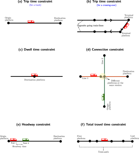
Figure 2: This figure graphically illustrates all the functional constraints present in a metro railway network that the timetable has to satisfy.

Trip time constraint

The trip time constraints are crucial in determining train energy consumption and regenerative energy production. As discussed previously, while a train is making a trip from the origin platform to the destination platform, almost all the its required energy is consumed during the acceleration phase of its trip and all of the regenerative braking energy is produced during the braking phase. Trip time constraints can be classified into two types described as follows.

Track-based trip time constraint.

Let us consider the trip of any train $t\in\mathcal{T}$ from platform $i$ to platform $j$ along the track $(i,j)\in\mathcal{A}^{t}$. The train departs from platform $i$ at time $d_{i}^{t}$, arrives at platform $j$ at time $a_{j}^{t}$, and its trip time can range from $\underline{\tau}_{ij}^{t}$ to $\overline{\tau}_{ij}^{t}$. We can express the trip time constraint as:

$$\underline{\tau}_{ij}^{t}\leq a_{j}^{t}-d_{i}^{t}\leq\overline{\tau}_{ij}^{t},\quad\textrm{for }(i,j)\in\mathcal{A}^{t},\,t\in\mathcal{T}.$$ (TRACK)

This constraint is shown in Figure 2(a).

Crossing-over-based trip time constraint.

A crossing-over is a directed arc that connects two train-lines, where a train-line is a directed path consisting of non-opposite platforms and non-opposite tracks. When a train turns around by traversing the crossing-over and starts traveling through another train-line after arriving at the terminal platform of a train-line, it is considered as two different trains by the railway management. Let $\varphi$ be the set of all crossing-overs where turn-around events occur. Suppose we consider any crossing-over $(i,j)\in\varphi$ where the platforms $i$ and $j$ are located on different train-lines. Let $\mathcal{B}_{ij}$ be the set of all train pairs involved in the corresponding turn-around events on the crossing-over $(i,j)$. Let $(t,t^{\prime})\in\mathcal{B}_{ij}$, where train $t\in\mathcal{T}$ turns around at platform $i$ by traveling through the crossing-over $(i,j)$, and beginning from platform $j$, starts traversing a different train-line as train $t^{\prime}\in\mathcal{T}\setminus{t}$. A time window $[\underline{\kappa}_{ij}^{tt^{\prime}},\overline{\kappa}_{ij}^{tt^{\prime}}]$ must be maintained between the departure of the train from platform $i$ (labeled as train $t$) and the arrival at platform $j$ (labeled as train $t^{\prime}$). The corresponding trip time constraint can be expressed as:

$$\underline{\kappa}_{ij}^{tt^{\prime}}\leq a_{j}^{t^{\prime}}-d_{i}^{t}\leq\overline{\kappa}_{ij}^{tt^{\prime}},\quad\textrm{for }(t,t^{\prime})\in\mathcal{B}_{ij},\,(i,j)\in\varphi.$$ (CROSS)

This constraint is shown in Figure 2(b).

Dwell time constraint

When a train $t\in\mathcal{T}$ arrives at a platform $i\in\mathcal{N}^{t}$, it dwells there for a certain time interval denoted by $[\underline{\delta}_{i}^{t},\overline{\delta}_{i}^{t}]$, during which passengers can embark or disembark. The train departs from the station once the dwell time has elapsed. The difference between the departure time $d_{i}^{t}$ and arrival time $a_{i}^{t}$ due to dwell time lies between $\underline{\delta}_{i}^{t}$ and $\overline{\delta}_{i}^{t}$. We can express the dwell time constraint as:

$$\underline{\delta}_{i}^{t}\leq d_{i}^{t}-a_{i}^{t}\leq\overline{\delta}_{i}^{t},\quad\textrm{for }i\in\mathcal{N}^{t},\,t\in\mathcal{T}.$$ (DWELL)

This constraint is illustrated in Figure 2(c). Note that the platform index $i$ is varied over all elements of the set $\mathcal{N}^{t}$ in Equation (DWELL). This is so because every train $t\in\mathcal{T}$ arrives at the first platform $\mathcal{N}^{t}(1)$ in its train-path either from the depot or by turning around from some other line, and departs from the final platform $\mathcal{N}^{t}(|\mathcal{N}^{t}|)$ to return to the depot or start as a new train on another line by turning around. Therefore, train $t$ dwells at all the platforms in $\mathcal{N}^{t}$.

Connection constraint

In some cases, there might not be a direct train between the origin and destination of a passenger. To address this issue, the railway management employs connecting trains at interchange stations. Let $\chi\subseteq\mathcal{N}\times\mathcal{N}$ be the set of platform pairs where passengers transfer between trains. If $(i,j)\in\chi$, then both platforms $i$ and $j$ are located at the same station, and there exists a train $t\in\mathcal{T}$ arriving at platform $i$ and another train $t^{\prime}\in\mathcal{T}$ departing from platform $j$, such that a connection time window must be maintained between trains $t$ and $t^{\prime}$ for passengers to transfer from the former to the latter. Note that order matters in this context. Let $\mathcal{C}_{ij}$ be the set of train pairs that enable passengers to make the corresponding connection or turn-around event for the platform pair $(i,j)\in\chi$. The connection constraint can be expressed as:

$$\underline{\chi}_{ij}^{tt^{\prime}}\leq d_{j}^{t^{\prime}}-a_{i}^{t}\leq\overline{\chi}_{ij}^{tt^{\prime}},\quad\textrm{for }(t,t^{\prime})\in\mathcal{C}_{ij},\,(i,j)\in\chi,$$ (CONNECT)

where $\underline{\chi}_{ij}^{tt^{\prime}}$ and $\overline{\chi}_{ij}^{tt^{\prime}}$ are the lower and upper bounds, respectively, of the time window required to achieve the described connection between the associated trains. The connection constraint is shown in Figure 2(d).

Headway constraint

In any railway network, a minimum amount of time is always maintained between the departures of consecutive trains, known as the headway time. Let $(i,j)\in\mathcal{A}$ be the track between two platforms $i$ and $j$, and let $\mathcal{H}_{ij}$ be the set of train pairs that move along that track successively in the order of their departures. Assume that train $t$ and train $t^{\prime}$ move along this track in the same direction, where $(t,t^{\prime})\in\mathcal{H}_{ij}$. Let $h_{i}^{tt^{\prime}}$ and $h_{j}^{tt^{\prime}}$ be the associated headway times at platforms $i$ and $j$, respectively. The headway constraint can be expressed as follows:

$$h_{i}^{tt^{\prime}}\leq d_{i}^{t^{\prime}}-d_{i}^{t}\;\textrm{ and }\ h_{j}^{tt^{\prime}}\leq d_{j}^{t^{\prime}}-d_{j}^{t},\quad\textrm{for }(t,t^{\prime})\in\mathcal{H}_{ij},\,(i,j)\in\mathcal{A}.$$ (HEADWAY)

The headway constraint is shown in Figure 2(e).

To ensure the safety of train operations, we must always maintain the headway constraints between two consecutive trains on the same track. Thus, when a train enters the braking phase and approaches a platform, the platform it enters cannot be immediately occupied by another train, as doing so would result in a temporal distance smaller than the headway time. It follows that selecting two consecutive trains, one accelerating and one braking at the same platform, is not feasible for synchronization from a safety standpoint. This underscores the importance of carefully considering the headway constraints when optimizing train schedules.

Total travel time constraint

In order to provide reliable service in the railway network, it is crucial to ensure that the total travel time for each train $t\in\mathcal{T}$ falls within a specified time window $[\underline{\tau}_{\mathcal{P}}^{t},\overline{\tau}_{\mathcal{P}}^{t}]$, where $\underline{\tau}_{\mathcal{P}}^{t}$ and $\overline{\tau}_{\mathcal{P}}^{t}$ are the corresponding lower and upper bounds, respectively. This means that the time elapsed between the train’s departure from its first platform $\mathcal{N}^{t}(1)$ and its arrival at the last platform $\mathcal{N}^{t}(|\mathcal{N}^{t}|)$ must lie within the prescribed time window. Mathematically, we can express this constraint as:

$$\underline{\tau}_{\mathcal{P}}^{t}\leq a_{\mathcal{N}^{t}(|\mathcal{N}^{t}|)}^{t}-d_{\mathcal{N}^{t}(1)}^{t}\leq\overline{\tau}_{\mathcal{P}}^{t},\quad\textrm{for }t\in\mathcal{T}.$$ (TRAVEL)

It is worth noting that violating this constraint could result in delayed trains, missed connections, and reduced overall network capacity. This constraint is shown in Figure 2(f).

Domain of the event times

We can define the domain of the decision variables for the railway scheduling problem using the start and end times of the railway service period. To simplify the problem, we set the time of the first event of the service period to zero seconds, which corresponds to the departure of the first train of the day from some platform. We can then obtain an upper bound for the final event of the railway service period, which is the arrival of the last train of the day at some platform, by setting all trip times and dwell times to their maximum possible values. Let this upper bound be denoted by a positive number $m$. Then, the domain of the decision variables can be expressed as follows:

$$0\leq a_{i}^{t}\leq m,\;0\leq d_{i}^{t}\leq m,\quad\textrm{for }i\in\mathcal{N}^{t}.$$ (DOMAIN)

Modeling the effective energy consumption

In this section, we discuss how we model the objective that minimizes the effective energy consumption of the railway network. The effective energy consumption is defined as the total energy consumed by all trains during their acceleration phases, denoted by $E^{\textrm{con}}$, minus the total regenerative braking energy transferred to such accelerating trains from eligible braking trains, denoted by $E^{\textrm{reg}}$. This is expressed as $E^{\textrm{con}}-E^{\textrm{reg}}$. We next discuss how we apply data-driven approaches to model $E^{\textrm{con}}$ in Section 4.1 and $E^{\textrm{reg}}$ in Section 4.2.

Modeling total consumed energy $E^{\textrm{con}}$

Relationship between energy consumption and the trip time constraint.

Trains primarily consume electrical energy during their acceleration phase while going from an origin to a destination platform. As such, trip time constraints critically influence both energy consumption and the production of regenerative energy in trains. Once the trip time gets fixed, the energy-optimal speed profile can be efficiently computed in CBTC systems. A variety of software tools, e.g., Train Kinetics, Dynamics, and Control (KDC) Simulator used in our research, can be employed for this purpose [26]. The KDC simulator, based on the strategies of acceleration, speed holding, coasting, and braking, calculates the speed profile. This method aligns with the theoretical optimal speed profile as presented in the monograph [12]. For a deeper dive into the calculation of optimal speed profiles, readers might consider the following papers [14, 10, 11, 15, 18], with a comprehensive review available in [2]. The speed profile of a train on a track, e.g., the top subfigure of Figure 1, dictates its electrical power consumption and regeneration, leading to its power versus time graph or power graph, as shown in the bottom subfigure of Figure 1.

Energy consumption of all trains.

We denote the total energy consumed by all trains by

$$\sum_{t\in\mathcal{T}}\sum_{(i,j)\in\mathcal{A}^{t}}\underbrace{E_{i,j,t}^{\textrm{con,tr}}}_{\begin{subarray}{c}\textrm{depends on }\\ \textrm{trip time }(a_{j}^{t}-d_{i}^{t})\end{subarray}}\quad+\sum_{(i,j)\in\varphi,(t,t^{\prime})\in\mathcal{B}_{i,j}}\underbrace{E_{i,j,t,t^{\prime}}^{\textrm{con,cr}}}_{\begin{subarray}{c}\textrm{depends on }\\ \textrm{trip time }(a_{j}^{t^{\prime}}-d_{i}^{t})\end{subarray}},$$

where $E_{i,j,t}^{\textrm{con,tr}}:\mathbb{R}_{++}\to\mathbb{R}_{++}$ is the energy consumed by a train $t\in\mathcal{T}$ during the acceleration phase of the trip from the origin platform $i$ to the destination platform $j$ with $(i,j)\in\mathcal{A}^{t}$; in a CBTC system, this function depends on the trip time $(a_{j}^{t}-d_{i}^{t})$. Similarly, $E_{i,j,t,t^{\prime}}^{\textrm{con,cr}}:\mathbb{R}_{++}\to\mathbb{R}_{++}$ is the energy consumed by train $t$ while traversing the crossing-over $(i,j)\in\varphi$; the energy is again consumed during the acceleration phase of $t$’s trip from the origin platform $i$ to destination platform $j$, where it gets labeled as the train $t^{\prime}$ i.e., $(t,t^{\prime})\in\mathcal{B}_{i,j}$. The trip time $a_{j}^{t^{\prime}}-d_{i}^{t}$ associated with this crossing-over is the argument of $E_{i,j,t,t^{\prime}}^{\textrm{con,cr}}$ in a CBTC system.

Figure 3: This figure graphically illustrates how the energy consumed by a train $t$ going from platform $i$ to $j$ on track $(i,j)$ varies as the trip time $a_{j}^{t}-d_{i}^{t}$ is varied. The longer range of trip time, while not practical for a metro railway network, is shown to illustrate the nonlinear nature of the consumed energy versus trip time in long inter-city travels that often span a few hours. On the other hand, the valid range of trip time in a metro network denoted by $[\underline{\tau}_{ij}^{t},\overline{\tau}_{ij}^{t}]$ is on the order of seconds, and in such a setup an affine approximation for the consumed energy can be reasonable.

Data-driven approach to model the energy consumption.

The exact analytical form of $E_{i,j,t}^{\textrm{con,tr}}$ or $E_{i,j,t,t^{\prime}}^{\textrm{con,cr}}$ might be intractable as suggested by [11, 6] and as shown qualitiatively in Figure 1. Regardless, these functions exhibit a consistent characteristic: they are monotonically decreasing with trip time. That is to say, if an optimal speed profile is adhered to, the functions become non-increasing as trip time increases, as supported by [21]. Notably, even in scenarios where trains are manually driven, potentially straying from optimal strategies, empirical evidence still supports the monotonic decrease in average energy consumption with increased trip time, as can be observed in [25, Figure 1]. Furthermore, gathering practical measurements for the energy function is straightforward, either by analyzing historical data or employing physics-based simulations. A crucial observation into CBTC-enabled metro railway networks is the tight margin by which trip time is permitted to vary in Equations (TRACK) and (CROSS): such variations are often on the order of seconds. This leads us to the following assumption:

Assumption 4.1.

The amount by which the trip time is allowed to vary is on the order of seconds, i.e., $\overline{\tau}_{ij}^{t}-\underline{\tau}_{ij}^{t}$ in (TRACK) and $\overline{\kappa}_{ij}^{tt^{\prime}}-\underline{\kappa}_{ij}^{tt^{\prime}}$ in (CROSS) are on the order of seconds.

Given the monotonically decreasing behavior of the energy function and Assumption 4.1, we can reasonably approximate the energy consumption functions as affine functions. This is qualitatively depicted in Figure 3 for track-based trip time constraints. Similar curves can be expected for crossing-over based trip time constraints. Our next objective is to derive the best affine approximation for energy consumed as a function of trip time. We’ll achieve this by employing a least-squares method to fit a straight line to the energy versus trip time data, where the data can come from historical records or physics-based simulators, such as the KDC simulator, which we used in this work [26].

In other words, we approximate consumed energy as:

$$E_{i,j,t}^{\textrm{con,tr}}\triangleq c_{i,j,t}^{\textrm{con,tr}}(a_{j}^{t}-d_{i}^{t})+b_{i,j,t}^{\textrm{con,tr}},\quad\textrm{for }(i,j)\in\mathcal{A}^{t},\,t\in\mathcal{T},$$ (1)

$$E_{i,j,t,t^{\prime}}^{\textrm{con,cr}}\triangleq c_{i,j,t,t^{\prime}}^{\textrm{con,cr}}(a_{j}^{t^{\prime}}-d_{i}^{t})+b_{i,j,t,t^{\prime}}^{\textrm{con,cr}},\quad\textrm{for }(i,j)\in\varphi,(t,t^{\prime})\in\mathcal{B}_{i,j},$$

where $(c_{i,j,t}^{\textrm{con,tr}},b_{i,j,t}^{\textrm{con,tr}})$ is computed by solving the following least-squares problem:

$$(c_{i,j,t}^{\textrm{con,tr}},b_{i,j,t}^{\textrm{con,tr}})=\textrm{argmin}_{(\tilde{c}_{i,j,t},\tilde{b}_{i,j,t})}\sum_{k=1}^{p}\left(\tilde{c}_{i,j,t}(a_{j}^{t}-d_{i}^{t})^{(k)}+\tilde{b}_{i,j,t}-(\bar{E}_{i,j,t}^{\textrm{con,tr}})^{(k)}\right)^{2},$$

where $(i,j)\in\mathcal{A}^{t},\,t\in\mathcal{T}$, with $(\bar{E}_{i,j,t}^{\textrm{con,tr}})^{(k)}$ being the measured energy consumption associated with the track related trip time $(a_{j}^{t}-d_{i}^{t})^{(k)}$ for observations $k=1,2,\ldots,p$. Similarly, $(c_{i,j,t,t^{\prime}}^{\textrm{con,cr}},b_{i,j,t,t^{\prime}}^{\textrm{con,cr}})$ is computed by solving the following least-squares problem:

$$(c_{i,j,t,t^{\prime}}^{\textrm{con,cr}},b_{i,j,t,t^{\prime}}^{\textrm{con,cr}})=\textrm{argmin}_{(\tilde{c}_{i,j,t,t^{\prime}},\tilde{b}_{i,j,t,t^{\prime}})}\sum_{k=1}^{q}\left(\tilde{c}_{i,j,t,t^{\prime}}(a_{j}^{t^{\prime}}-d_{i}^{t})^{(k)}+\tilde{b}_{i,j,t,t^{\prime}}-(\bar{E}_{i,j,t,t^{\prime}}^{\textrm{con,cr}})^{(k)}\right)^{2},$$

where $(i,j)\in\varphi,(t,t^{\prime})\in\mathcal{B}_{i,j}$ with $\bar{E}{}_{i,j,t,t^{\prime}}^{\textrm{con,cr}}{}^{(k)}$

being the measured energy consumption related to crossing-over related trip time $(a_{j}^{t^{\prime}}-d_{i}^{t})^{(k)}$ for observations $k=1,2,\ldots,q$.

Modeling transferred regenerative energy $E^{\textrm{reg}}$

Robust approximations of the power vs. time graph.

Maximizing the transfer of regenerative braking energy between suitable train pairs is equivalent to maximizing the total overlapped area between the power vs. time graphs associated with power consumption and regeneration of those train pairs. The power vs. time graph for a train during its acceleration and braking phases depends on its trip time and is highly nonlinear in nature with no known analytical form in CBTC systems. However, the graph empirically exhibits a region where most of the power is concentrated, which allows us to apply the robust lumping method known as the FWHM (Full Width at Half Maximum) method, approximating the power vs. time graphs as rectangles. The FWHM method can be traced back to the early days of quantum mechanics [8], where it was instrumental in approximating the wave absorption vs. wavelength graph of molecules [7, Chapter 5], and since then it has been used successfully in various fields such as numerical analysis, spectroscopy, signal processing, and statistics to approximate complicated graphs, and it’s considered a useful, robust metric because it is not sensitive to the exact shape of the peak [20, pp. 35-37]. In the context of our problem, the FWHM method is applied by transforming the power vs. time graph into a rectangle (see Figure 4) whose height is the height of the peak and whose width is the full width at half maximum. These rectangles allow us to recognize the beginning and end of a train’s effective accelerating or braking phases where most of the energy is concentrated, which we illustrate graphically in Figure 4.

Consider a train $t$ arriving at (i.e., braking), then dwelling, and finally departing (i.e., accelerating) from platform $i$. As shown in Figure 4, the effective braking and accelerating phases of the train can be compactly contained in FWHM rectangle. We denote the beginning and end of the effective braking phase of $t$ by $a_{i}^{t}-\underline{\beta}_{i}^{t}$ and $a_{i}^{t}-\overline{\beta}_{i}^{t}$, respectively, and the beginning and end of the effective accelerating phase of the train $t$ by $d_{i}^{t}+\underline{\alpha}_{i}^{t}$ and $d_{i}^{t}+\overline{\alpha}_{i}^{t}$, respectively.

Determining the beginning and end of the effective braking and accelerating phases of the trains allows us to model the effective overlapping time in a very compact way. The effective overlapping time between two trains is defined as the duration of time during which the effective accelerating phase of the first train and the effective braking phase of the second train overlap, provided that both trains are powered by the same electrical substation, and the transmission loss associated with the transfer of regenerative energy of the braking train to the accelerating train is negligible. Thus, maximizing the transfer of regenerative energy positively correlates with the effective overlapping time between suitable train pairs, which we model next.

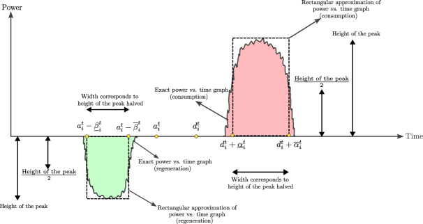
Figure 4: This figure illustrates how to compute the effective braking and acceleration phases of trains using the FWHM (Full Width at Half Maximum) method. Consider a train $t$ arriving (i.e., braking) at, then dwelling, and finally departing (i.e., accelerating) from platform $i$. While the exact power vs. time graph of a train is challenging to model analytically, it is possible to compute a very robust approximation by applying the FWHM method. By doing so, the effective braking and accelerating phase of a train can be compactly represented by these rectangular approximations, which allows us to identify the beginning and end of the effective braking phase of train $t$, denoted by $a_{i}^{t}-\underline{\beta}_{i}^{t}$ and $a_{i}^{t}-\overline{\beta}_{i}^{t}$, respectively, and the beginning and end of the effective accelerating phase of the train $t$, represented by $d_{i}^{t}+\underline{\alpha}_{i}^{t}$ and $d_{i}^{t}+\overline{\alpha}_{i}^{t}$, respectively.

Constructing suitable train pairs for transfer of regenerative braking energy.

The set that contains all platform pairs that are feasible for regenerative energy transfer is denoted by $\Omega$. Consider any such platform pair $(i,j)\in\Omega$, and let $\mathcal{T}_{i}\subseteq\mathcal{T}$ be the set of all the trains that arrive at, dwell and then depart from platform $i$. To avoid duplicates in $\Omega$ we construct the elements lexicographically with $i<j$. Suppose, $t\in\mathcal{T}_{i}$. Now, we are interested in finding another train $\tilde{t}$ on platform $j$, i.e., $\tilde{t}\in\mathcal{T}_{j}$, which along with $t$ would form a suitable pair for the transfer of regenerative braking energy. To achieve this, we start with an initial feasible timetable for the railway, which represents the desired service to be delivered. For most of the existing railway networks, the railway management has a feasible timetable. For every train $t$, this feasible timetable provides a feasible arrival time $\bar{a}_{i}^{t}$ and a feasible departure time $\bar{d}_{i}^{t}$ to and from every platform $i\in\mathcal{N}^{t}$ respectively. Intuitively, among all the trains that go through platform $j$, the one that is temporally close to $t$ in the initial timetable would be a good candidate to form a pair with $t$. The temporal proximity can be of two types with respect to $t$, which results in the following definitions.

Definition 4.1.

Consider any $(i,j)\in\Omega$. For every train $t\in\mathcal{T}_{i}$, the train $\overset{\rightharpoonup}{t}\in\mathcal{T}_{j}$ is called temporally close to the right of $t$ if $0\leq\frac{\bar{a}_{j}^{\overset{\rightharpoonup}{t}}+\bar{d}_{j}^{\overset{\rightharpoonup}{t}}}{2}-\frac{\bar{a}_{i}^{t}+\bar{d}_{i}^{t}}{2}\leq r$, where $r$ is an empirical parameter determined by the timetable designer and is much smaller than the time horizon of the entire timetable.

Definition 4.2.

Consider any $(i,j)\in\Omega$. For every train $t\in\mathcal{T}_{i}$, the train $\overset{\leftharpoonup}{t}\in\mathcal{T}_{j}$ is called temporally close train to the left of $t$ if $0<\frac{\bar{a}_{i}^{t}+\bar{d}_{i}^{t}}{2}-\frac{\bar{a}_{j}^{\overset{\leftharpoonup}{t}}+\bar{d}_{j}^{\overset{\leftharpoonup}{t}}}{2}\leq r$.

Definition 4.3.

Consider any $(i,j)\in\Omega$. For every train $t\in\mathcal{T}_{i}$, the train $\tilde{t}\in\mathcal{T}_{j}$ is called temporally close to $t$ if it is temporally close to the left or right of $t$.

So, any event where transfer of regenerative energy is possible can be described by specifying the corresponding $i$, $j$, $t\in\mathcal{T}_{i}$ and $\tilde{t}\in\mathcal{T}_{j}$ by using the definitions above. We construct a set of all such $(i,j,t,\tilde{t})$ with $i<j$ (to avoid duplicates), which we denote by $\mathcal{E}$. Naturally, we can partition $\mathcal{E}$ into two sets denoted by $\overset{\rightharpoonup}{\mathcal{E}}$ and $\overset{\leftharpoonup}{\mathcal{E}}$, which contain elements of the form $(i,j,t,\overset{\rightharpoonup}{t})$ and $(i,j,t,\overset{\leftharpoonup}{t})$ respectively. For every $(i,j,t,\overset{\rightharpoonup}{t})\in\overset{\rightharpoonup}{\mathcal{E}}$ (called right event), our strategy is to synchronize the effective accelerating phase of $t$ with the effective braking phase of $\overset{\rightharpoonup}{t}$. On the other hand, for every $(i,j,t,\overset{\leftharpoonup}{t})\in\overset{\leftharpoonup}{\mathcal{E}}$ (called left event), it is convenient to synchronize the effective accelerating phase of $\overset{\leftharpoonup}{t}$ with the effective braking phase of $t$. For every $(i,j,t,\overset{\rightharpoonup}{t})\in\overset{\rightharpoonup}{\mathcal{E}}$, the corresponding effective overlapping time is denoted by $\sigma_{ij}^{t\overset{\rightharpoonup}{t}}$, (called right event overlapping time) and for every $(i,j,t,\overset{\leftharpoonup}{t})\in\overset{\leftharpoonup}{\mathcal{E}}$, the corresponding effective overlapping time is denoted by $\sigma_{ij}^{t\overset{\leftharpoonup}{t}}$ (called left event overlapping time). The overlapping time can be: positive when there is a positive temporal synchronization between effective acceleration phase and effective braking phase, zero where there is no synchronization and the temporal distance between the phases is zero, or negative which corresponds to the case where their phases are apart by a certain temporal distance; we will illustrate these different overlapping times graphically later in this section.

The total regenerative energy transferred depends on the total effective overlapping time. Our objective is to maximize the transfer of regenerative energy, which we model by:

$$\sum_{(i,j,t,\overset{\rightharpoonup}{t})\in\overset{\rightharpoonup}{\mathcal{E}}}\underbrace{E_{i,j,t,\overset{\rightharpoonup}{t}}^{\textrm{reg}}}_{\begin{subarray}{c}\textrm{depends on }\\ \textrm{right event }\\ \textrm{overlapping time }\sigma_{ij}^{t\overset{\rightharpoonup}{t}}\end{subarray}}\quad+\sum_{(i,j,t,\overset{\leftharpoonup}{t})\in\overset{\leftharpoonup}{\mathcal{E}}}\underbrace{E_{i,j,t,\overset{\leftharpoonup}{t}}^{\textrm{reg}}}_{\begin{subarray}{c}\textrm{depends on }\\ \textrm{left event }\\ \textrm{overlapping time }\sigma_{ij}^{t\overset{\leftharpoonup}{t}}\end{subarray}},$$ (2)

where (i) $E_{i,j,t,\overset{\rightharpoonup}{t}}^{\textrm{reg}}:\mathbb{R}\to\mathbb{R}$ measures the transfer of regenerative energy from synchronizing the accelerating phase of $t$ with the braking phase of $\overset{\rightharpoonup}{t}$, with the associated overlapping time $\sigma_{ij}^{t\overset{\rightharpoonup}{t}}$ being the argument, (ii) $E_{i,j,t,\overset{\leftharpoonup}{t}}^{\textrm{reg}}:\mathbb{R}\to\mathbb{R}$ measures the transfer of regenerative energy from synchronizing the accelerating phase of $\overset{\leftharpoonup}{t}$ with the braking phase of $t$, where $\sigma_{ij}^{t\overset{\leftharpoonup}{t}}$ is the argument. To model (2) in a tractable manner, we perform three steps as follows: Step 1. Computing data-driven approximations of $E_{i,j,t,\overset{\rightharpoonup}{t}}^{\textrm{reg}}$ and $E_{i,j,t,\overset{\leftharpoonup}{t}}^{\textrm{reg}}$, Step 2. Computing data-driven approximations of the effective accelerating and braking phases of trains, and Step 3. Modeling the overlapping times. Next, we describe the three aforementioned steps in detail.

Step 1. Computing data-driven approximations of $E_{i,j,t,\overset{\rightharpoonup}{t}}^{\textrm{reg}}$ and $E_{i,j,t,\overset{\leftharpoonup}{t}}^{\textrm{reg}}$.

Using a data-driven approach, we approximate $E_{i,j,t,\overset{\rightharpoonup}{t}}^{\textrm{reg}}$ and $E_{i,j,t,\overset{\rightharpoonup}{t}}^{\textrm{reg}}$ as affine functions of effective overlapping time $\sigma_{ij}^{t\overset{\rightharpoonup}{t}}$ and $\sigma_{ij}^{t\overset{\leftharpoonup}{t}},$ respectively. Due to Assumption 4.1, it is again reasonable to approximate the transferred regenerative energy functions as affine functions of the effective overlapping time. In other words, we denote:

$$E_{i,j,t,\overset{\rightharpoonup}{t}}^{\textrm{reg}} \triangleq c_{i,j,t,\overset{\rightharpoonup}{t}}^{\textrm{reg}}\sigma_{ij}^{t\overset{\rightharpoonup}{t}}+b_{i,j,t,\overset{\rightharpoonup}{t}}^{\textrm{reg}},$$ (3)

$$E_{i,j,t,\overset{\leftharpoonup}{t}}^{\textrm{reg}} \triangleq c_{i,j,t,\overset{\leftharpoonup}{t}}^{\textrm{reg}}\sigma_{ij}^{t\overset{\leftharpoonup}{t}}+b_{i,j,t,\overset{\leftharpoonup}{t}}^{\textrm{reg}},$$

where $(c_{i,j,t,\overset{\rightharpoonup}{t}}^{\textrm{reg}},b_{i,j,t,\overset{\rightharpoonup}{t}}^{\textrm{reg}})$ and $(c_{i,j,t,\overset{\leftharpoonup}{t}}^{\textrm{reg}},b_{i,j,t,\overset{\leftharpoonup}{t}}^{\textrm{reg}})$ are positive coefficients computed via a constrained least squares problem where our input measurement data corresponds to effective overlapping time with output measurement data corresponds to the transferred regenerative braking energy. This measurement data can come from either historical data or physics-based simulation; in our numerical experiments, this data is generated by the KDC simulator. The positive values of $b_{i,j,t,\overset{\rightharpoonup}{t}}^{\textrm{reg}}$ and $b_{i,j,t,\overset{\leftharpoonup}{t}}^{\textrm{reg}}$ denote residual transfer of regenerative energy. This may occur due to some energy lying outside of our FWHM rectangles, even when the overlapping time is zero. Our affine modeling of $E_{i,j,t,\overset{\rightharpoonup}{t}}^{\textrm{reg}}$ and $E_{i,j,t,\overset{\leftharpoonup}{t}}^{\textrm{reg}}$ in (3) leads to the interpretation of the objective in (2), which we aim to maximize. Because the coefficients $(c_{i,j,t,\overset{\rightharpoonup}{t}}^{\textrm{reg}},b_{i,j,t,\overset{\rightharpoonup}{t}}^{\textrm{reg}})$, $(c_{i,j,t,\overset{\leftharpoonup}{t}}^{\textrm{reg}},b_{i,j,t,\overset{\leftharpoonup}{t}}^{\textrm{reg}})$ are nonnegative, positive overlappings would always lead to a positive transfer of regenerative energy. However, a negative or zero overlapping $\sigma_{ij}^{t\overset{\rightharpoonup}{t}}$ (or $\sigma_{ij}^{t\overset{\leftharpoonup}{t}}$) may have some small transfer of regenerative energy. For $\sigma_{ij}^{t\overset{\rightharpoonup}{t}}\leq-b_{i,j,t,\overset{\rightharpoonup}{t}}^{\textrm{reg}}/c_{i,j,t,\overset{\rightharpoonup}{t}}^{\textrm{reg}}$ (or $\sigma_{ij}^{t\overset{\leftharpoonup}{t}}\leq-b_{i,j,t,\overset{\leftharpoonup}{t}}^{\textrm{reg}}/c_{i,j,t,\overset{\leftharpoonup}{t}}^{\textrm{reg}}$), there will be little to no transfer of regenerative energy. In those cases, the negative values of $E_{i,j,t,\overset{\rightharpoonup}{t}}^{\textrm{reg}}$ (or $E_{i,j,t,\overset{\leftharpoonup}{t}}^{\textrm{reg}}$) introduce a penalty that reduces the value of the objective (2) being maximized. We make this modeling decision of introducing this penalty rather than setting the regenerative energy to zero directly because even when the overlapping time is negative, it is preferable to have the absolute value as small as possible. This approach aims to achieve some residual synchronization by reducing the penalty.

Step 2. Computing data-driven approximations of the effective accelerating and braking phases of trains.

To compute the effective overlapping time, we need to compute the beginning and end of the effective accelerating and braking phases of the trains. Consider the trip of any train $t\in\mathcal{T}$ from platform $i$ to platform $j$ along the track $(i,j)\in\mathcal{A}^{t}$. The beginning and end of the effective accelerating phase of $t$ while departing from platform $i$ is denoted by by $d_{i}^{t}+\underline{\alpha}_{i}^{t}$ and $d_{i}^{t}+\overline{\alpha}_{i}^{t}$ respectively. Similarly, the beginning and end of the effective braking phase of $t$ while arriving at platform $j$ by $a_{j}^{t}-\underline{\beta}_{j}^{t}$ and $a_{j}^{t}-\overline{\beta}_{j}^{t}$, respectively. The values for $\underline{\alpha}_{i}^{t},\overline{\alpha}_{i}^{t},\underline{\beta}_{j}^{t},\overline{\beta}_{j}^{t}$ depend on the power graph of the train, which in turn depends on the trip time $a_{j}^{t}-d_{i}^{t}$. Analytical approximations of the aforementioned terms as a function of $a_{j}^{t}-d_{i}^{t}$ for a given train are not known, however, due to Assumption 4.1, it is reasonable to work with affine approximations of the trip times. So, for $t\in\mathcal{T}$, and $(i,j)\in\mathcal{A}^{t}$, we define $\underline{\alpha}_{i}^{t},\overline{\alpha}_{i}^{t},\underline{\beta}_{j}^{t},\overline{\beta}_{j}^{t}$ as follows:

$$\underline{\alpha}_{i}^{t} \triangleq c_{i,t}^{\underline{\alpha}}(a_{j}^{t}-d_{i}^{t})+b_{i,t}^{\underline{\alpha}},\quad\overline{\alpha}_{i}^{t}\triangleq c_{i,t}^{\overline{\alpha}}(a_{j}^{t}-d_{i}^{t})+b_{i,t}^{\overline{\alpha}},$$ (EFF_ACCEL_&_BRK_PHASES)

$$\underline{\beta}_{j}^{t} \triangleq c_{i,t}^{\underline{\beta}}(a_{j}^{t}-d_{i}^{t})+b_{i,t}^{\underline{\beta}},\quad\overline{\beta}_{j}^{t}\triangleq c_{i,t}^{\overline{\beta}}(a_{j}^{t}-d_{i}^{t})+b_{i,t}^{\overline{\beta}},$$

where the coefficients $(c_{i,t}^{\underline{\alpha}},b_{i,t}^{\underline{\alpha}})$, $(c_{i,t}^{\overline{\alpha}},b_{i,t}^{\overline{\alpha}})$, $(c_{i,t}^{\underline{\beta}},b_{i,t}^{\underline{\beta}}),$ and $(c_{i,t}^{\overline{\beta}},b_{i,t}^{\overline{\beta}})$ are computed via least-squares with input measurement data corresponds to trip time with output measurement data corresponds to the beginning or end of the effective acceleration and braking phases.

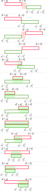
Figure 5: This figure illustrates all the possible overlapping times $\sigma_{ij}^{t\overset{\rightharpoonup}{t}}$. For the first four cases, $\sigma_{ij}^{t\overset{\rightharpoonup}{t}}$ shown using the red-shaded region is nonpositive, whereas for the next nine cases $\sigma_{ij}^{t\overset{\rightharpoonup}{t}}$ is positive shown using the green-shaded region. The overlapping time $\sigma_{ij}^{t\overset{\rightharpoonup}{t}}$ admits the closed form $\min\left\{a_{j}^{\overset{\rightharpoonup}{t}}-\overline{\beta}_{j}^{\overset{\rightharpoonup}{t}},d_{i}^{t}+\overline{\alpha}_{i}^{t}\right\}+\min\left\{-d_{i}^{t}-\underline{\alpha}_{i}^{t},-a_{j}^{\overset{\rightharpoonup}{t}}+\underline{\beta}_{j}^{\overset{\rightharpoonup}{t}}\right\}$.

Step 3. Modeling the overlapping times.

Now, we describe how to model the effective overlapping time $\sigma_{ij}^{t\overset{\rightharpoonup}{t}}$ and $\sigma_{ij}^{t\overset{\leftharpoonup}{t}}$ in terms of the decision variables present in the system.

First, we discuss the modeling of right event overlapping time $\sigma_{ij}^{t\overset{\rightharpoonup}{t}}$. Using Allen’s interval algebra [3], we know that there can be thirteen different kinds of overlapping possible between the accelerating phase of train $t$ and the braking phase of train $\overset{\rightharpoonup}{t}$ as shown in Figure 5. For the first four cases shown in Figure 5, the overlapping is nonpositive, i.e., the temporal blocks are apart from each other by a nonpositive distance (which is shown in the red-shaded region), whereas for the next nine cases, there is a positive overlapping in time (which is shown using the green-shaded region). Fortunately, we can write all these thirteen possible overlapping times in a closed form:

$$\sigma_{ij}^{t\overset{\rightharpoonup}{t}} =\min\left\{a_{j}^{\overset{\rightharpoonup}{t}}-\overline{\beta}_{j}^{\overset{\rightharpoonup}{t}},d_{i}^{t}+\overline{\alpha}_{i}^{t}\right\}-\max\left\{d_{i}^{t}+\underline{\alpha}_{i}^{t},a_{j}^{\overset{\rightharpoonup}{t}}-\underline{\beta}_{j}^{\overset{\rightharpoonup}{t}}\right\}$$

$$=\min\left\{a_{j}^{\overset{\rightharpoonup}{t}}-\overline{\beta}_{j}^{\overset{\rightharpoonup}{t}},d_{i}^{t}+\overline{\alpha}_{i}^{t}\right\}+\min\left\{-d_{i}^{t}-\underline{\alpha}_{i}^{t},-a_{j}^{\overset{\rightharpoonup}{t}}+\underline{\beta}_{j}^{\overset{\rightharpoonup}{t}}\right\}$$ (RGHT_EVNT_OVLP_TIME)

which is a concave function in the decision variables $a_{j}^{\overset{\rightharpoonup}{t}}$, $d_{i}^{t},\overline{\alpha}_{i}^{t}$, $\underline{\alpha}_{i}^{t}$, $\underline{\beta}_{j}^{\overset{\rightharpoonup}{t}}$, and $\overline{\beta}_{j}^{\overset{\rightharpoonup}{t}}$, as it is a pointwise minimum of affine functions in the decision variables, which preserves concavity [4, Section 3.2]. Next, we discuss modeling of left event overlapping time $\sigma_{ij}^{t\overset{\leftharpoonup}{t}}$. Similar to the first case, we can write $\sigma_{ij}^{t\overset{\leftharpoonup}{t}}$ as (easily proved by replacing $i$, $j$, $t$ and $\overset{\rightharpoonup}{t}$ in $\sigma_{ij}^{t\overset{\rightharpoonup}{t}}$ with $j$, $i$, $\overset{\leftharpoonup}{t}$ and $t$ respectively)

$$\sigma_{ij}^{t\overset{\leftharpoonup}{t}} =\min\left\{a_{i}^{t}-\overline{\beta}_{i}^{t},d_{j}^{\overset{\leftharpoonup}{t}}+\overline{\alpha}_{j}^{\overset{\leftharpoonup}{t}}\right\}-\max\left\{d_{j}^{\overset{\leftharpoonup}{t}}+\underline{\alpha}_{j}^{\overset{\leftharpoonup}{t}},a_{i}^{t}-\underline{\beta}_{i}^{t}\right\}$$

$$=\min\left\{a_{i}^{t}-\overline{\beta}_{i}^{t},d_{j}^{\overset{\leftharpoonup}{t}}+\overline{\alpha}_{j}^{\overset{\leftharpoonup}{t}}\right\}+\min\left\{-d_{j}^{\overset{\leftharpoonup}{t}}-\underline{\alpha}_{j}^{\overset{\leftharpoonup}{t}},-a_{i}^{t}+\underline{\beta}_{i}^{t}\right\},$$ (LEFT_EVNT_OVLP_TIME)

which is a again concave function in our decision variables.

Final optimization model

Using our developments in the previous sections, we arrive at the following final linear optimization model to minimize the effective energy consumption of the railway network:

$$\underset{}{\mbox{minimize}}$$ (OPT_MODEL)

$$\sum_{t\in\mathcal{T},(i,j)\in\mathcal{A}^{t}}\left(c_{i,j,t}^{\textrm{con,tr}}(a_{j}^{t}-d_{i}^{t})+b_{i,j,t}^{\textrm{con,tr}}\right)\;+\quad\sum_{(i,j)\in\varphi,(t,t^{\prime})\in\mathcal{B}_{i,j}}\left(c_{i,j,t,t^{\prime}}^{\textrm{con,cr}}(a_{j}^{t^{\prime}}-\quad d_{i}^{t})+b_{i,j,t,t^{\prime}}^{\textrm{con,cr}}\right)\quad\rhd\;\textrm{consumption}$$

$$-\quad\sum_{(i,j,t,\overset{\rightharpoonup}{t})\in\overset{\rightharpoonup}{\mathcal{E}}}\left(c_{i,j,t,\overset{\rightharpoonup}{t}}^{\textrm{reg}}\sigma_{ij}^{t\overset{\rightharpoonup}{t}}+b_{i,j,t,\overset{\rightharpoonup}{t}}^{\textrm{reg}}\right)\;-\sum_{(i,j,t,\overset{\leftharpoonup}{t})\in\overset{\leftharpoonup}{\mathcal{E}}}\left(c_{i,j,t,\overset{\leftharpoonup}{t}}^{\textrm{reg}}\sigma_{ij}^{t\overset{\leftharpoonup}{t}}+b_{i,j,t,\overset{\leftharpoonup}{t}}^{\textrm{reg}}\right)\quad\rhd\;\textrm{transferred regen. energy}$$

subject to

$$\begin{rcases}\sigma_{ij}^{t\overset{\rightharpoonup}{t}}\leq\varpi_{ij}^{t\overset{\rightharpoonup}{t}}+\varphi_{ij}^{t\overset{\rightharpoonup}{t}},\quad\textrm{for }(i,j,t,\overset{\rightharpoonup}{t})\in\overset{\rightharpoonup}{\mathcal{E}}\\ \varpi_{ij}^{t\overset{\rightharpoonup}{t}}\leq a_{j}^{\overset{\rightharpoonup}{t}}-\overline{\beta}_{j}^{\overset{\rightharpoonup}{t}},\quad\textrm{for }(i,j,t,\overset{\rightharpoonup}{t})\in\overset{\rightharpoonup}{\mathcal{E}}\\ \varpi_{ij}^{t\overset{\rightharpoonup}{t}}\leq d_{i}^{t}+\overline{\alpha}_{i}^{t},\quad\textrm{for }(i,j,t,\overset{\rightharpoonup}{t})\in\overset{\rightharpoonup}{\mathcal{E}}\\ \varphi_{ij}^{t\overset{\rightharpoonup}{t}}\leq-d_{i}^{t}-\underline{\alpha}_{i}^{t},\quad\textrm{for }(i,j,t,\overset{\rightharpoonup}{t})\in\overset{\rightharpoonup}{\mathcal{E}}\\ \varphi_{ij}^{t\overset{\rightharpoonup}{t}}\leq-a_{j}^{\overset{\rightharpoonup}{t}}+\underline{\beta}_{j}^{\overset{\rightharpoonup}{t}},\quad\textrm{for }(i,j,t,\overset{\rightharpoonup}{t})\in\overset{\rightharpoonup}{\mathcal{E}}\end{rcases}\begin{subarray}{c}\rhd\;\textrm{hypograph}\\ \textrm{constraints }\\ \textrm{for}\eqref{eq:sigma_right}\end{subarray}$$

$$\begin{rcases}\sigma_{ij}^{t\overset{\leftharpoonup}{t}}\leq\varpi_{ij}^{t\overset{\leftharpoonup}{t}}+\varphi_{ij}^{t\overset{\leftharpoonup}{t}},\quad\textrm{for }(i,j,t,\overset{\leftharpoonup}{t})\in\overset{\leftharpoonup}{\mathcal{E}}\\ \varpi_{ij}^{t\overset{\leftharpoonup}{t}}\leq a_{i}^{t}-\overline{\beta}_{i}^{t},\quad\textrm{for }(i,j,t,\overset{\leftharpoonup}{t})\in\overset{\leftharpoonup}{\mathcal{E}}\\ \varpi_{ij}^{t\overset{\leftharpoonup}{t}}\leq d_{j}^{\overset{\leftharpoonup}{t}}+\overline{\alpha}_{j}^{\overset{\leftharpoonup}{t}},\quad\textrm{for }(i,j,t,\overset{\leftharpoonup}{t})\in\overset{\leftharpoonup}{\mathcal{E}}\\ \varphi_{ij}^{t\overset{\leftharpoonup}{t}}\leq-d_{j}^{\overset{\leftharpoonup}{t}}-\underline{\alpha}_{j}^{\overset{\leftharpoonup}{t}},\quad\textrm{for }(i,j,t,\overset{\leftharpoonup}{t})\in\overset{\leftharpoonup}{\mathcal{E}}\\ \varphi_{ij}^{t\overset{\leftharpoonup}{t}}\leq-a_{i}^{t}+\underline{\beta}_{i}^{t},\quad\textrm{for }(i,j,t,\overset{\leftharpoonup}{t})\in\overset{\leftharpoonup}{\mathcal{E}}\\ \end{rcases}\begin{subarray}{c}\rhd\;\textrm{hypograph}\\ \textrm{constraints }\\ \textrm{for}\eqref{eq:sigma_left}\end{subarray}$$

$$\textrm{Eq.}\;\eqref{eq:effective_braking_accelearation_compute},\quad\rhd\;\textrm{beginning and end of acceleration and braking}$$

$$\textrm{Eq.}\;\eqref{eq:TripTimeConstraint},\eqref{eq:turnAroundConstraint},\eqref{eq:DwellTimeConstraint},\eqref{eq:ConnectionConstraint},\eqref{eq:SafetyConstraint1},\eqref{eq:TotalTravelTimeConstraints},\;\rhd\;\textrm{operational constraints}$$

$$\textrm{Eq.}\;\eqref{eq:domain},\;\rhd\;\textrm{domain of decision variable}$$

where the decision variables are $a_{i}^{t}$, $d_{i}^{t}$, $\sigma_{ij}^{t\overset{\rightharpoonup}{t}},$$\varpi_{ij}^{t\overset{\rightharpoonup}{t}},$ $\varphi_{ij}^{t\overset{\rightharpoonup}{t}}$, $\sigma_{ij}^{t\overset{\leftharpoonup}{t}},$ $\varpi_{ij}^{t\overset{\leftharpoonup}{t}},$ and $\varphi_{ij}^{t\overset{\leftharpoonup}{t}}$. Note that the first ten constraints recast (RGHT_EVNT_OVLP_TIME) and (LEFT_EVNT_OVLP_TIME) as linear constraints using the hypograph approach [4, Section 4.1.3].

Predicting effective energy consumption from the solution.

Once we have computed an optimal solution to (OPT_MODEL), it provides us with the energy-optimal timetable. An estimate of the effective energy consumption of the final timetable is given by:

$$\sum_{t\in\mathcal{T},(i,j)\in\mathcal{A}^{t}}\left(c_{i,j,t}^{\textrm{con,tr}}(a_{j}^{t}-d_{i}^{t})+b_{i,j,t}^{\textrm{con,tr}}\right)\;\quad+\sum_{(i,j)\in\varphi,(t,t^{\prime})\in\mathcal{B}_{i,j}}\left(c_{i,j,t,t^{\prime}}^{\textrm{con,cr}}(a_{j}^{t^{\prime}}-d_{i}^{t})+b_{i,j,t,t^{\prime}}^{\textrm{con,cr}}\right)$$

$$-\sum_{(i,j,t,\overset{\rightharpoonup}{t})\in\overset{\rightharpoonup}{\mathcal{E}}}\max\left\{c_{i,j,t,\overset{\rightharpoonup}{t}}^{\textrm{reg}}\sigma_{ij}^{t\overset{\rightharpoonup}{t}}+b_{i,j,t,\overset{\rightharpoonup}{t}}^{\textrm{reg}},0\right\}\;\quad-\sum_{(i,j,t,\overset{\leftharpoonup}{t})\in\overset{\leftharpoonup}{\mathcal{E}}}\max\left\{c_{i,j,t,\overset{\leftharpoonup}{t}}^{\textrm{reg}}\sigma_{ij}^{t\overset{\leftharpoonup}{t}}+b_{i,j,t,\overset{\leftharpoonup}{t}}^{\textrm{reg}},0\right\},$$ (PRED_EFF_ENG_CNSM)

where the first line computes the energy consumption during the acceleration, whereas the second line is the negative of the actual transfer of regenerative energy, thus the final expression corresponds to the predicted effective energy consumption. Recall that when $\sigma_{ij}^{t\overset{\rightharpoonup}{t}}\leq 0$ and $\sigma_{ij}^{t\overset{\leftharpoonup}{t}}\leq 0$, the summands $c_{i,j,t,\overset{\rightharpoonup}{t}}^{\textrm{reg}}\sigma_{ij}^{t\overset{\rightharpoonup}{t}}+b_{i,j,t,\overset{\rightharpoonup}{t}}^{\textrm{reg}}$ and $c_{i,j,t,\overset{\leftharpoonup}{t}}^{\textrm{reg}}\sigma_{ij}^{t\overset{\leftharpoonup}{t}}+b_{i,j,t,\overset{\leftharpoonup}{t}}^{\textrm{reg}}$ act as penalty terms in the objective function of (OPT_MODEL), so $\max\{c_{i,j,t,\overset{\rightharpoonup}{t}}^{\textrm{reg}}\sigma_{ij}^{t\overset{\rightharpoonup}{t}}+b_{i,j,t,\overset{\rightharpoonup}{t}}^{\textrm{reg}},0\}$ and $\max\{c_{i,j,t,\overset{\leftharpoonup}{t}}^{\textrm{reg}}\sigma_{ij}^{t\overset{\leftharpoonup}{t}}+b_{i,j,t,\overset{\leftharpoonup}{t}}^{\textrm{reg}},0\}$ correspond to the actual transferred regenerative energy for the individual events, respectively.

Numerical experiment

This section has the following organization. In Section 6.1, we describe the railway network where we apply our model. In Section 6.2, we present the results of our numerical study.

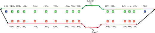
Figure 6: Railway network considered for the numerical study.

Railway network in consideration

Our empirical analysis focuses on Metro Line 8 of the Shanghai Railway network, a critical component of the world’s most extensive metro system by route length. The Shanghai Railway Network also stands second in terms of station count while leading in global metro ridership with approximately 3.88 billion passengers served in 2019 [30]. The Metro Line 8 infrastructure, in particular, traverses some of Shanghai’s highest-density residential areas and records an average daily ridership of about 1.08 million. The line spans 37.4 km and encompasses 28 functional stations [31]. Metro Line 8 features three distinct services, each governed by individually optimized timetables generated through communication-based train control systems. In this study, we formulate energy-efficient timetables specifically for the $\textrm{PES}_{2}$-$\textrm{SFM}_{2}$ service route within Metro Line 8, as depicted in Figure 6. The said network is composed of two lines—Line 1 and Line 2—with 14 stations represented in all uppercase in the figure. Notably, each station comprises dual platforms catering to trains from both lines; for instance, LXM Station includes platforms $\textrm{LXM}_{1}$ and $\textrm{LXM}_{2}$, which serve Line 1 and Line 2, respectively. The line under examination has a total length of 37 km. The stations have an average inter-station distance of 1.4 km, ranging from a minimum of 738 m (between YHR and ZJD) to a maximum of 2.6 km (between PJT and LHR). Operational constraints are subject to well-defined physical limits, including the track slope, which lies within the range of $[-2.00453^{\circ},2.00453^{\circ}]$, and the maximum permissible acceleration and deceleration of trains, specified as 1.04 $\textrm{m/s}^{2}$ and -0.8 $\textrm{m/s}^{2}$, respectively. The conversion efficiency from electrical to kinetic energy is 0.9, and from kinetic to regenerative braking energy is 0.76, as well as the transmission loss factor of regenerative electricity is 0.1.

Results of the numerical study

To compute the energy-efficient timetables for the $\textrm{PES}_{2}$-$\textrm{SFM}_{2}$ service on Shanghai Railway Network’s Metro Line 8, we consider 11 distinct operational instances. Each instance encompasses unique parameters, including train count, headway durations, train velocities, track gradients, and energy consumption profiles during acceleration and braking phases. Thales Canada Inc. has provided us with existing timetables corresponding to these 11 scenarios. Upon the computation of our energy-optimized timetables, we quantify the improvements by comparing the energy usage against these baseline timetables.

Table 2: Results of the numerical study applied Metro Line 8 of Shanghai Railway Network.

#Trains	#Variables	#Constraints	Solution time (s)	Initial effective energy consumption (kWh)	Predicted final effective energy consumption (kWh)	Reduction predicted by our model (%)	Reduction predicted by SPSIM (%)
1000	47581	151259	0.669	353721.62	252282.87	28.68	30.27
1032	49104	156102	0.674	364832.93	263288.46	27.83	31.34
1066	50726	161254	0.731	376017.98	271346.61	27.84	33.04
1100	52339	166391	0.683	386087.42	284325.21	26.36	29.10
1132	53865	171239	0.760	389844.65	291664.27	25.18	26.56
1166	55487	176391	0.753	407717.20	301714.07	26.00	26.55
1198	57010	181234	0.763	417767.32	330319.76	20.93	19.27
1232	58626	186376	0.855	447025.23	334638.29	25.14	25.86
1266	60242	191518	0.867	438657.08	332747.39	24.14	26.94
1298	61765	196361	0.901	449379.24	333858.16	25.71	24.83
1332	63387	201513	0.906	475354.59	350642.67	26.24	25.97

The computational experiments were conducted on a desktop computer comprising an AMD Ryzen 9 7950X CPU with 16 cores and 32 threads, accompanied by 32 GB of RAM, and operating on a Windows 11 Pro platform. We employed the algebraic modeling language JuMP, a state-of-the-art, open-source framework, to articulate our optimization problem [19]. Within this framework, we implemented the parallel interior-point algorithm of the Gurobi Optimizer 10.0 [9]. To accelerate the optimization process, we initialized the algorithm using existing timetables generously supplied by Thales Canada Inc, significantly reducing the computational time required to reach an optimal solution.

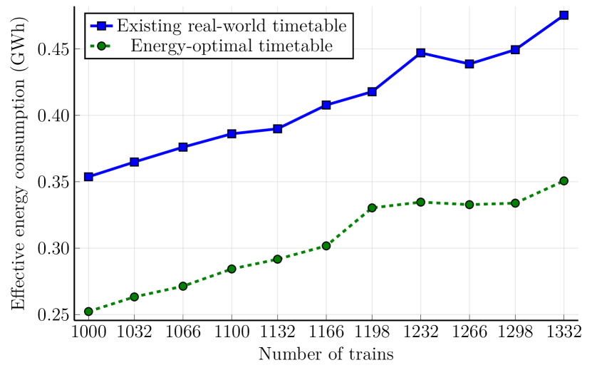
(a)

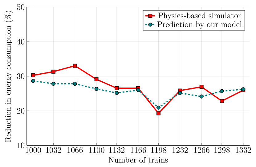
(b)

Figure 7: Figure 7(a) compares the predicted effective energy consumption of the energy-optimal timetables (prediction by (PRED_EFF_ENG_CNSM)) to that of the existing real-world timetables. Figure 7(b) shows that the reduction predicted by our model is quite close to proprietary physics-based simulator SPSIM.

The findings of this computational study are encapsulated in Table 2. In every scenario, the solution time was confined to less than one second, effectively rendering the model amenable to real-time applications. The baseline effective energy consumption metrics, associated with the initial timetables, were ascertained through SPSIM, a physics-based simulation tool utilized by Thales Canada Inc. Upon obtaining the optimal solution, as formulated in equation (OPT_MODEL), we proceeded to evaluate the effective energy consumption of the optimized timetables utilizing equation (PRED_EFF_ENG_CNSM). The optimized timetables demonstrated a substantial improvement over their real-world counterparts, with the reductions in effective energy consumption spanning from approximately 20.93% in the least favorable instances to as much as 28.68% in the most advantageous cases. This is also graphically illustrated in Figure 7(a).

To corroborate the validity of our model’s predictions, we conducted a comparative analysis with the physics-based simulator SPSIM. The latter’s estimates were generated by inputting our optimized timetables into the simulator, calculating the resultant effective energy consumption and subsequently the degree of reduction. The comparative metrics, enumerated in the last two columns of Table 2 and Figure 7(b), reveal a strong alignment between the two prediction methodologies, although our model tends to yield slightly more conservative estimates on average. The variance can be attributed to the methodology employed by SPSIM for computing the transfer of regenerative energy, which is based on the precise area of overlap between power-versus-time graphs for pairs of accelerating and decelerating trains. This may occasionally exceed the energy transfer estimates provided by our model, which employs rectangular approximations of these graphs, as delineated in Section 4.2.

Architectural framework for industrial integration of the proposed model

This section describes the architectural framework that facilitates the incorporation of the optimization model proposed in this paper into Thales Canada Inc’s industrial timetable compiler. As shown in Figure 8, the core architecture has two primary constituents: (i) the existing timetable compiler, showcased on the left, and (ii) the energy-optimal timetable generator, represented on the right.

For the purpose of this integration framework, the existing timetable compiler is partitioned into three discrete modules:

• Timetable data: This module houses the necessary data to solve the optimization problem. Additionally, it includes other information specific to the railway network under consideration, such as gradient attributes and speed limitations in various track segments; all presented in their raw form.

• Optimization class: This module transforms the raw data into a structure that is compatible with the optimization algorithm we employ.

• CSCPP class: This class establishes a bi-directional communication link between the industrial timetable compiler and the energy-optimal timetable generator. It injects the input data into the optimization algorithm, retrieves the optimized timetable, and converts it into a format amenable for deployment in a communication-based train control system.

The energy-optimal timetable generator is similarly sub-divided into three modules:

• Type definitions: This module contains the data structures essential for describing a railway network, as previously elaborated in Sections 3 and 5.

• Utility functions: This module contains the critical functions required for the optimization algorithm’s operation. Included are the description of the optimization model (OPT_MODEL), a function to predict effective energy consumption via (PRED_EFF_ENG_CNSM), and another to transform the output timetable in a CSCPP-compatible format.

• Optimization algorithm: This segment contains the parallel interior-point algorithm used for solving (OPT_MODEL), supplemented by a warm-start mechanism. Once the final timetable is computed, the algorithm forwards the results to the CSCPP class through the utility functions.

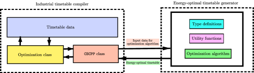
Figure 8: The architecture for integrating our optimization model with an industrial timetable compiler

Conclusion

In this paper, we have proposed a novel single-stage linear optimization model to compute energy-optimal timetables for sustainable communication-based train control systems. Our model simultaneously minimizes the total energy consumption of all trains and maximizes the transfer of regenerative braking energy. Distinct from existing models, that are either NP-hard or require multi-stage simulations, our model facilitates real-time decision-making by producing energy-optimal timetables subject to the inherent functional constraints of metro railway networks. We demonstrated the model’s impact via its application to Shanghai Railway Network’s Metro Line 8, achieving energy savings between 20.93% and 28.68% in comparison with existing real-world timetables, with sub-second computational times on a standard desktop. Given its managerial implications and computational robustness, our model is poised for global implementation as an integrated component of Thales Canada Inc’s timetable compiler.

References

- [1] M Abril, F Barber, L Ingolotti, MA Salido, P Tormos, and A Lova. An assessment of railway capacity. Transportation Research Part E: Logistics and Transportation Review, 44(5):774–806, 2008.
- [2] Amie Albrecht, Phil Howlett, Peter Pudney, Xuan Vu, and Peng Zhou. The key principles of optimal train control - part 1: Formulation of the model, strategies of optimal type, evolutionary lines, location of optimal switching points. Transportation Research Part B: Methodological, 94:482–508, 2016.
- [3] James F Allen. Maintaining knowledge about temporal intervals. Communications of the ACM, 26(11):832–843, 1983.
- [4] Stephen Boyd and Lieven Vandenberghe. Convex optimization. Cambridge university press, 2009.
- [5] Shuvomoy Das Gupta, Lacra Pavel, and James Kevin Tobin. An optimization model to utilize regenerative braking energy in a railway network. In American Control Conference (ACC), 2015.
- [6] Shuvomoy Das Gupta, J Kevin Tobin, and Lacra Pavel. A two-step linear programming model for energy-efficient timetables in metro railway networks. Transportation Research Part B: Methodological, 93:57–74, 2016.
- [7] Max Diem. Quantum Mechanical Foundations of Molecular Spectroscopy. John Wiley & Sons, 2021.
- [8] George Gamow. Thirty years that shook physics: The story of quantum theory. Courier Corporation, 1985.
- [9] Gurobi Optimization, LLC. Gurobi Optimizer Reference Manual, 2023.
- [10] Phil Howlett. The optimal control of a train. Annals of Operations Research, 98:65–87, 2000.
- [11] Phil G Howlett, Peter J Pudney, and Xuan Vu. Local energy minimization in optimal train control. Automatica, 45(11):2692–2698, 2009.
- [12] Philip G Howlett and Peter J Pudney. Energy-efficient train control. Springer Science & Business Media, 1995.
- [13] IRSE International Technical Committee. Semi-automatic, driverless, and unattended operation of trains. Available at: http://tinyurl.com/2k2u3ktv, 2009.
- [14] Cheng Jiaxin and Phil Howlett. A note on the calculation of optimal strategies for the minimization of fuel consumption in the control of trains. IEEE Transactions on Automatic Control, 38(11):1730–1734, 1993.
- [15] Eugene Khmelnitsky. On an optimal control problem of train operation. IEEE transactions on automatic control, 45(7):1257–1266, 2000.
- [16] Zhao Le, Keping Li, Jingjing Ye, and Xiaoming Xu. Optimizing the train timetable for a subway system. Proceedings of the Institution of Mechanical Engineers, Part F: Journal of Rail and Rapid Transit, 2014.
- [17] Xiang Li and Hong K Lo. An energy-efficient scheduling and speed control approach for metro rail operations. Transportation Research Part B: Methodological, 64:73–89, 2014.
- [18] Rongfang Rachel Liu and Iakov M Golovitcher. Energy-efficient operation of rail vehicles. Transportation Research Part A: Policy and Practice, 37(10):917–932, 2003.
- [19] Miles Lubin, Oscar Dowson, Joaquim Dias Garcia, Joey Huchette, Benoît Legat, and Juan Pablo Vielma. JuMP 1.0: Recent improvements to a modeling language for mathematical optimization. Mathematical Programming Computation, 2023.
- [20] Sanjoy Mahajan. Street-fighting mathematics: the art of educated guessing and opportunistic problem solving. The MIT Press, 2010.
- [21] Ian P Milroy. Aspects of automatic train control. PhD thesis, Loughborough University, 1980.
- [22] Ahmed Mohamed, Andrew Reid, and Thomas Lamb. White paper on wayside energy storage for regenerative braking energy recuperation in the electric rail system. Con Edison: New York, NY, USA, pages 1–20, 2018.
- [23] Robert D Pascoe and Thomas N Eichorn. What is communication-based train control? IEEE Vehicular Technology Magazine, 4(4):16–21, 2009.
- [24] Maite Peña-Alcaraz, Antonio Fernández, Asuncion Paloma Cucala, Andres Ramos, and Ramon R Pecharromán. Optimal underground timetable design based on power flow for maximizing the use of regenerative-braking energy. Proceedings of the Institution of Mechanical Engineers, Part F: Journal of Rail and Rapid Transit, 226(4):397–408, 2012.
- [25] Maite Pena Alcaraz, Mort Webster, and Andrés Ramos. An approximate dynamic programming approach for designing train timetables. 2011.
- [26] Thales Canada Inc. SelTrac communications-based train control for urban rail. https://www.thalesgroup.com/en/communications-based-train-control-cbtc-signalling, 2023.
- [27] United Nations. World urbanization prospects. https://esa.un.org/unpd/wup/Publications/Files/WUP2014-Report.pdf, 2014.
- [28] Pengling Wang and Rob MP Goverde. Multi-train trajectory optimization for energy efficiency and delay recovery on single-track railway lines. Transportation Research Part B: Methodological, 105:340–361, 2017.
- [29] Pengling Wang and Rob MP Goverde. Multi-train trajectory optimization for energy-efficient timetabling. European Journal of Operational Research, 272(2):621–635, 2019.
- [30] Wikipedia. Description of shanghai metro network. https://en.wikipedia.org/wiki/Shanghai_Metro, 2023. Online; Wikipedia, The Free Encyclopedia.
- [31] Wikipedia. Line 8 (shanghai metro). https://en.wikipedia.org/wiki/Line_8_(Shanghai_Metro), 2023. Online; Wikipedia, The Free Encyclopedia.
- [32] Songpo Yang, Feixiong Liao, Jianjun Wu, Harry JP Timmermans, Huijun Sun, and Ziyou Gao. A bi-objective timetable optimization model incorporating energy allocation and passenger assignment in an energy-regenerative metro system. Transportation Research Part B: Methodological, 133:85–113, 2020.