A conformal test of linear models via permutation-augmented regressions
Abstract
Permutation tests are widely recognized as robust alternatives to tests based on normal theory. Random permutation tests have been frequently employed to assess the significance of variables in linear models. Despite their widespread use, existing random permutation tests lack finite-sample and assumption-free guarantees for controlling type I error in partial correlation tests. To address this ongoing challenge, we have developed a conformal test through permutation-augmented regressions, which we refer to as PALMRT. PALMRT not only achieves power competitive with conventional methods but also provides reliable control of type I errors at no more than , given any targeted level , for arbitrary fixed designs and error distributions. We have confirmed this through extensive simulations.
Compared to the cyclic permutation test (CPT) and residual permutation test (RPT), which also offer theoretical guarantees, PALMRT does not compromise as much on power or set stringent requirements on the sample size, making it suitable for diverse biomedical applications. We further illustrate the differences in a long-Covid study where PALMRT validated key findings previously identified using the t-test after multiple corrections, while both CPT and RPT suffered from a drastic loss of power and failed to identify any discoveries. We endorse PALMRT as a robust and practical hypothesis test in scientific research for its superior error control, power preservation, and simplicity. An R package for PALMRT is available at https://github.com/LeyingGuan/PairedRegression.
Key words: Partial correlation; Random permutation; Assumption-free; Conformal test.
1 Introduction
Consider a linear regression model
| (1) |
with features and , and random errors independent of . Testing whether the coefficient is zero in this linear model, or equivalently, examining the partial correlation between and , remains a fundamental statistical query and a prevalent approach in applications like biological signature discovery. For instance, a key question in the recent MY-LC study is whether long-COVID (LC) is associated with specific cell type proportions, after adjusting for age, sex, and Body Mass Index (BMI) (Klein et al., 2023) :
| (2) |
While the F/t-test is a standard approach (Fisher, 1922; Fisher et al., 1924; Fisher, 1970), it may yield anti-conservative p-values under ill-behaved error distributions or limited sample sizes, compromising the reliability of scientific discoveries. Therefore, there is a need for a valid hypothesis test that minimizes assumptions on the noise distribution and does not rely on asymptotic theory. Motivated by this, we seek a robust and straightforward testing procedure for partial correlation under the sole assumption of exchangeability.
Assumption 1.1.
The noise variables are exchangeable with in law.
The problem of testing partial correlations has been intensively studied, with a focus on developing various random permutation methods to increase robustness against diverse noise distributions. Draper and Stoneman (1966) introduced a permutation technique for partial correlation testing, referred to as PERMtest, which involves permuting alone and disrupts the relationship between and . Subsequent methods better accounted for this relationship. A family of methods, such as the Freedman and Lane test (FLtest) (Freedman and Lane, 1983) and the Kennedy-test (Kennedy, 1995), permutes response residuals obtained from a reduced model that regresses on . Another type of method, such as the Braak-test (Ter Braak, 1992), shuffles residuals from a full model regressing on both and . These methods have demonstrated empirically robust type I error control in various benchmark studies when using pivotal test statistics like t-test or F-test statistics (Hall and Wilson, 1991; Westfall and Young, 1993; Anderson and Robinson, 2001; Winkler et al., 2014). However, finite-sample and assumption-free theoretical guarantees for these random permutation tests remain elusive. This contrasts with permutation tests for simple correlation, which are theoretically sound in terms of type I error control (Pitman, 1937; Manly, 2006; Edgington and Onghena, 2007). Indeed, even the widely-examined and recommended FLtest can, under specific conditions, yield drastically inflated type I error rates, as we demonstrate later.
Recently, Lei and Bickel (2021) introduced the cyclic permutation test (CPT), which offers worst-case guarantees for controlling type I error. Given a sample size and a total feature dimension for , CPT theoretically ensures type I error control at a target level , provided . This condition is often challenging to meet in biomedical studies. For instance, in immunology research, sample sizes frequently hover around 100 or a few hundreds, while investigating simultaneously hundreds or even more different biomarkers for their partial correlations with a primary feature of interest. Although applying CPT with a cutoff may suffice with fewer concomitant covariates, the situation complicates when multiple hypothesis corrections are applied, as smaller nominal -value thresholds are needed to maintain a reasonable false discovery rate (FDR). In an independent pursuit of robust partial correlation analysis with increased power and reduced sample size, Wen et al. (2022) introduces the residual permutation test (RPT), defined under the condition . This test utilizes a sequence of specially-designed permutation matrices, which, in conjunction with the identity matrix, form a group. However, there’s a trade-off in the choice of the size parameter : a small permutation set size limits testing for small p-values, while a large reduces RPT power significantly by design (see Table 1). Obtaining a sequence of well-designed permutation matrices with a reasonable size, such as as suggested by Wen et al. (2022), remains challenging for small . Following the proposed RPT Algorithm Wen et al. (2022), a non-trivial test requires .
In this manuscript, we develop PALMRT, which stands for Permutation-Augmented Linear Model Regression Test, as a conformal test to examine the partial correlation relationships in a linear model. Unlike traditional random permutation methods, PALMRT not only empirically controls type I error but also theoretically guarantees a worst-case coverage of at any targeted error level . It offers well-calibrated -values for finite-sample type I error control under arbitrary fixed designs or noise distributions. Table 1 provides a brief summary of different methods regarding their construction, empirical performance, theoretical guarantee, and dimension constraints for non-trivial rejection under the i.i.d random Gaussian design.
In our empirical analyses, PALMRT not only maintains empirical Type I error rates below the designated thresholds across diverse simulation settings but also exhibits comparable power to established methods like FLtest when is moderately large. It significantly outperforms CPT and RPT in commonly encountered scenarios. Upon re-analyzing the MY-LC study, PALMRT validates the top findings from the original study, while CPT and RPT show reduced discoveries and fail to confirm any main findings after multiple test corrections. Consequently, we recommend adopting PALMRT as the default robust procedure for detecting significant partial correlations in our daily research.
In our empirical analyses, PALMRT not only maintains empirical Type I error rates below the designated thresholds across diverse simulation settings but also exhibits comparable power to established methods like FLtest when is moderately large and outperforms CPT in commonly encountered scenarios. Upon re-analyzing the MY-LC study, we confirmed the robustness of the top findings from the original study using PALMRT. Consequently, we advocate for the adoption of PALMRT as a robust default procedure for detecting significant partial correlations in our daily research.
Method Original Model Permuted Model Empirical Worst-Case Restriction PERMtest FLtest Kenny-test Braak-test CPT RPT PALMRT
2 Conformal test via permutation-augmented regressions
2.1 Construction of PALMRT
Let be the target feature, and the observation matrix with rows . Define as the vector and as a permutation of . Denote and as the row-permuted versions of and respectively. PALMRT is a random permutation method for testing partial correlation. For each randomly generated permutation of , it constructs “original” and “permuted test” statistics based on a pair of permutation-augmented regressions:
-
•
Original test statistic : the F-statistic for significance of in the model :
-
•
Permuted test statistic : the F-statistic for significance of in the model :
Here, denotes the projection matrix onto the column space of its argument . For instance, represents the projection matrix onto the column space of , onto that of , etc. We have more confidence of having non-zero if is larger than . One can easily verify that comparing and is equivalent to comparing the following simplified expressions on the fitted residuals:
| (3) |
We adopt eq. (3) to construct the original and permuted statistics for any given permutation. Subsequently, we generate random permutations of uniformly and compare the associated original and permuted statistics to compute the p-value for testing . The complete procedure is outlined in Algorithm 1.
2.2 An example differentiating FLtest and PALMRT
We offer an illustrative example, see Example 2.1, to demonstrate PALMRT’s superior robustness compared to FLtest. Although FLtest has been lauded for its type I error control in prior studies, it may fail under extreme noise and design configurations. In contrast, PALMRT consistently maintains type I error control.
Example 2.1.
We set and , and examine a special design where , . We generate the response under the global null as , where , denoted as “multinomial noise.” This extreme noise scenario serves as a robustness test. The feature design represents an imbalanced ANOVA setup with many control samples but only one sample per treatment group. Even though exact permutation is feasible by shuffling the zero rows, we employ standard FLtest and PALMRT to evaluate their empirical coverage using 2000 random draws of . Figure 1A shows the miscoverage ratio, defined as
As the targeted level becomes small, FLtest encountered excessively inflated type I error – more than 10-fold that of the targeted level when . In contrast, PALMRT controls type I error for small . Figures 1B-C are the histograms of p-values using FLtest and PALMRT. The distribution of p-values from FLtest contains a spike close to 0, leading to its type I error inflation.
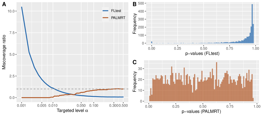
Example 1 is a distinguishing example where FLtest suffers from being severely anti-conservative for small but PALMRT continues to offer robust type I error control. This robustness of PALMRT is universally true. In the next section, we will show that PALMRT, as well as a family of other permutation tests based on paired constructions, guarantees a maximum type I error of , irrespective of the noise distribution, design, and sample size.
3 Type I error control guarantee
In this section, we establish that PALMRT provides finite-sample type I error guarantees under any design and exchangeable noise. This property is generalized to a family of tests that performs comparisons with paired statistics as realizations of a specially-designed bi-variate function on permutation orders.
Under the null hypothesis , PALMRT essentially compares a bi-variate function across two given permutations and their swaps. Specifically, for any two permutations and of , we define a bi-variate function, which also incorporates data , , and unobserved noise as model parameters, as follows:
| (4) |
Let be the identity permutation of .
Proposition 3.1.
Under the null hypothesis , the statistic pair are realizations of evaluated at and respectively:
Many existing random permutation tests, including FLtest and PERMtest, can be expressed as realizations of such bi-variate functions. For example, construct bi-variate functions and defined below,
Let denote the original statistic and represent permuted test statistics. Under , it can be verified via direct calculation that are realizations at and of or for PERMtest and FLtest respectively, with the second argument in the bivariate functions being inactive.
What sets apart and enables its theoretical guarantee? The crucial distinction between and or lies in the transferability of permutations from the noise parameter to its permutation arguments. This property holds uniquely for across all noise realizations and designs. Let be an arbitrary permutation of and its inverse, such that with denoting composition. Then, any permutation of the parameters in can be expressed equivalently as applying the inverse permutation to the permutation arguments and .
Proposition 3.2.
The application of a permutation to is equivalent to applying the permutation to , in :
Proposition 3.2 is derived from simple term rearrangement, and we omit its proof here. This transferability property is pivotal for establishing the type I error guarantees. In fact, for any paired statistics which can be considered as realizations of a bi-variate function at and under , the resulting p-value from comparing to offers a theoretical guarantee as long as satisfies the transferability condition 3.1, as outlined in Theorem 3.3.
Condition 3.1.
For any permutations of , the function satisfies
Theorem 3.3.
Remark 3.4.
Interestingly, the empirical version of RPT, discussed independently in Wen et al. (2022), is also a realization of paired constructions described in Theorem 3.3 when is full rank for different permutations , by setting
This leads to the comparison between and , which can be easily verified. In Wen et al. (2022), the authors recognized the power issue with RPT and introduced this empirical version to enhance power. However, it lacks theoretical justification. Here, we demonstrate also that the empirical RPT has a strong theoretical foundation as a special case of Theorem 3.3 and is a version of PALMRT by replacing the pivotal statistics with residuals inner product, hence, the requirement on permutations by RPT is unnecessary in its context.
The worst-case bound established in Theorem 3.3 aligns with the bounds for prediction coverage established for multisplit conformal prediction methods including CV+, Jackknife+, and ensemble conformal predictions (Vovk et al., 2018; Barber et al., 2021; Kim et al., 2020; Gupta et al., 2022; Han et al., 2023). However, our focus diverges significantly as we concentrate on hypothesis testing for the true model parameter rather than an out-of-sample prediction. Traditional exchangeability arguments, applicable when predicting on new samples, are inadequate for assessing the significance of . To tackle this, we employ new arguments exploiting the assumption of exchangeable noise. A proof sketch for Theorem 3.3 is provided below.
Proof sketch of Theorem 3.3.
One key insight is that, when considering both the randomness in the permutations and , the matrix , with its -th entry as , is distributionally equivalent to whose -th entry is with independently and uniformly generated from the permutation space of . This equivalence allows us to analyze the p-value from Algorithm 1 by examining corresponding entries in .
Define . Then, corresponds to the numerator when constructing , the p-value in Algorithm 1, upon substituting with . Since are i.i.d. generated, we expect to be exchangeable for different . Thus, we can bound by bounding the size of the index set , which can be obtained following similar arguments used in proving prediction interval’s coverage for multi-split conformal prediction. ∎
Theorem 3.3 is the main theoretical result of this work, and we include its full proof in Section 5. Combining Theorem 3.3 with Proposition 3.2, we concludes that Algorithm 1 theoretically controls type I error, albeit with a relaxed upper bound of .
Of note, unlike existing random permutation tests where the use of pivotal statistics is often crucial, Theorem 3.3 generalizes beyond pivotal statistics, allowing for other non-pivotal paired constructions. For example, could be the absolute value of the regression coefficients of and in the models and respectively. For directional tests, the test statistics may employ either the regression coefficients (for positive effects) or their negations (for negative effects).
4 An Exact Confidence Interval Construction
In conjunction with the PALMRT -value, a confidence interval for can be constructed by inverting the test. Define as the test statistics from replacing by in Algorithm 2 when constructing . Define as , where .
Corollary 4.1.
Set where and . Then, we have , for all .
Remark 4.2.
The set obtained through directly inverting , is often an interval, but not always guaranteed to be so. By taking the infimum and supremum of this set, we obtain a confidence interval with worst-case guarantee at least as strong as direct inversion.
The pertinent question remaining is the efficient computation of the confidence interval as delineated in Corollary 4.1. Traditional methods for constructing the confidence interval in permutation tests typically rely on normal theory, Bootstrap (Efron, 1987; Efron and Tibshirani, 1994; DiCiccio and Efron, 1996; Davison and Hinkley, 1997), or grid search (Garthwaite, 1996). Here, we provide an exact formulation of via examining critical values, derived from pair-wise comparisons at each permutation . First, we observe that the contribution from the term to the numerator is explicitly known.
Lemma 4.3.
Set , , , and . Then, we have and
| (5) |
where and .
As a result, we first partition of index set of into three sets , , and . The value of remains constant as we vary for . Hence, the requirement of is equivalent to imposing a requirement on that captures the contribution of , as shown below:
It can be shown that the function value of is characterized by comparing to different values for :
| (6) |
Let denote the ordered values of unique elements in , and let represent the sizes of and , respectively. As we increase in, the function value can only changes when we first hit , or when slightly increases from these critical values represented. We represent the concept of increasing slightly from these critical values by , where indicates being infinitesimally larger than . Using these new quantities introduced, we can re-express and identify induction relations for the function values as we increase to surpass the critical values , described as follows:
| (7) |
We can utilize eq. (7) to efficiently calculate all and in time, given and . Acquisition of the matrix , and can be done in time if we record intermediate quantities from Algorithm 1. Consequently, efficient comparisons between with to determine and can be achieved. Algorithm 2 presents full details of this implementation, and provides exact construction of as stated in Theorem 4.4.
Theorem 4.4.
Remark 4.5.
The confidence interval can potentially be an empty set (). Although this does not invalidate our assertion, an empty set offers limited information in practical contexts and might not be desired. In such situations, we may pt to construct the confidence interval using a normal approximation in the regression whenever Algorithm 2 produces an empty set as the output for .
5 Proof of Theorem 3.3
Before conducting numerical experiments comparing PALMRT and existing methods, we provide the full proof to Theorem 3.3 in this section. We define as the permutation space of , as the permutation space of , as the unordered value set of (duplicates are allowed). Proposition 5.1 is useful for establishing our exchangeability statement. Proposition 5.2 is a minor modification of arguments for bounding “strange set” used in proving multi-splitting conformal prediction.
Proposition 5.1.
Let and be generated independently and uniformly from . Then and are also generated independently and uniformly from .
Proof.
First, it is obvious that is uniformly generated from since the map is a bijection between and itself. Hence, by definition, for any permutations of , we have
| (8) |
where the last two steps have used the fact that and are independent and uniformly from . Eq (8) is the definition for and being independent and uniformly generated from . ∎
Proposition 5.2.
Let be any matrix, and the comparison matrix where for and . Let be the row sum of . Then, for all , we have
Proof.
Notice that (1) for all , , and (2) for all . For any sub-square matrix of constructed from selecting the same columns and rows (denoted the index set as ), we have
Set . Suppose the size of is . The corresponding rows in must implicate:
This concludes our proof. ∎
5.1 Proof to Theorem 3.3
On the one hand, under Assumption 1.1 and conditional on the value sets , generation of can be characterized by generating independently and uniformly generated from .
On the other hand, by Condition 3.1 and denoting as the identity permutation of , we have
| (9) | ||||
Here, we have dropped the parameters and in for convenience.
Write , , …, , by eq. (9) and Proposition 5.1, the marginalized joint distribution of the B pairs of statistics conditional only on can be re-expressed equivalently (in distribution) using :
| (10) |
where are independently and uniformly generated from , and can be viewed as fixed. Hence, setting , to understand the behavior of the constructed p-value using , we can equivalently consider the distribution of :
Now, we complete the full matrix by setting for all . We also set the comparison matrix of as described in Proposition 5.2 and set . Then, by Proposition 5.2, the size of is upper bounded and .
Note that the p-value constructed using is
To avoid confusion, we use the lower case to denote the observed row sums given the current realizations , and be the random variables as we change the permutations . Then, conditional on the unordered set of permutations , the observed permutations take the form , for , where is a permutation of . Since are i.i.d generated from , is uniformly generated from the .
The above results can be used to derive the exchangeability among conditional on and . Notice that when is permuted according to , the row sum is permuted accordingly:
Combining the above display with the fact that is uniform from , we conclude that are exchangeable. Consequently, we have
6 Numerical Experiments
We evaluate the performance and type I error control of various methods through numerical experiments, setting the sample size at , and varying the dimension of in . We investigate four designs: i.i.d Gaussian, i.i.d Cauchy, balanced ANOVA where each feature takes roughly an equal number of non-overlapping 1s, and a paired design where each feature assumes a value of 1 at two entries and 0 elsewhere, with one unique and one shared one-valued entry across all features. We also consider three noise settings: Gaussian, Cauchy, and multinomial. The paired design and multinomial noise distributions are atypical in real-world applications and are included as challenging test cases for evaluating the robustness of FLtest, which has demonstrated commendable empirical performance under more conventional design structures and noise distributions in existing literature.
We compare our proposed PALMRT against six existing methods:(1) F-test, (2) PERMtest, (3) FLtest, (4) CPT with strong pre-odering by the genetic algorithm as per Lei and Bickel (2021), (5) RPT, and (6) Bias-corrected and Accelerated Bootstrap, previously favored over plain Bootstrap (Efron, 1987; Diciccio and Romano, 1988; Hall, 1988; DiCiccio and Efron, 1996). All comparisons were conducted at the p-value cut-off in the main paper; PALMRT’s type I error control is further explored for and in supplementary materials.
For random permutation tests (PALMRT, FLtest, PERMtest), we employed F-statistics as the test statistics and set the permutation count . Bias-corrected and Accelerated Bootstrap and CPT can be more time-intensive. We used bcaboot R package with 500 bootstraps and 20 jackknife blocks (Efron and Narasimhan, 2020). For CPT, we used the implementation from the authors’ GitHub, followed the strong ordering approach with 10,000 optimization steps via genetic algorithms, and set the number of cyclic permutations as 19 (corresponding to ) (Lei and Bickel, 2021). For RPT, we used the implementation provided by the authors and set the the number of permutation as 19 (corresponding to ) as recommended (Wen et al., 2022).
We generated 2,000 independent noise instances for each experimental setting and used them to compute empirical type I error, statistical power, and confidence intervals across various signal-to-noise ratios. Sections 6.1 and 6.2 compare type I error and power among F-test, PERMtest, FLtest, CPT, RPT, and PALMRT. Section 6.3 examines CI coverage for and their median lengths from independent runs using normal theory, Bootstrap and Algorithm 2.
6.1 Type I error control
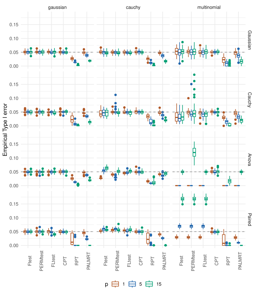
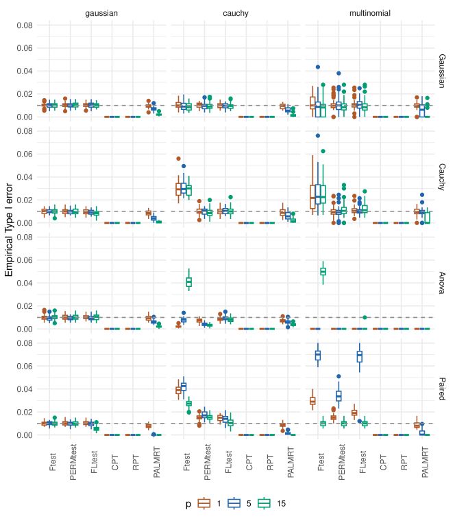
To empirically assess type I error control, we simulate the global null distribution with . Figure 2 displays type I errors from 50 independent repetitions for each setting using F-test, PERMtest, FLtest, CPT, RPT and PALMRT.
In the Gaussian noise or the Gaussian/Cauchy design contexts, all methods effectively control type I errors. However, for ANOVA or Paired designs, Ftest, FLtest, and PERMtest yield inflated type I errors when noise is non-Gaussian – especially pronounced in the Paired design with multinomial errors. This underscores that not only F-test, but also FLtest and PERMtest, lack distribution-free theoretical guarantees and can be anti-conservative in finite-sample settings.
Among the methods tested, only PALMRT, CPT and RPT guarantee worst-case coverage across all experimental settings. Although CPT’s accurate type I error control is by design for , its accuracy in other settings was somewhat unexpected. For example, in the Gaussian design where , the cyclic invariant constraints of CPT can only be satisfied by a constant vector with high probability, leading to a trivial test that always accepts . Further examination indicates that these observations arise because cyclic-invariant constraints of CPT are not perfectly satisfied in the implemeted CPT, thereby permitting non-constant . PALMRT demonstrates empirical type I errors close to or below target levels, while RPT, as noted in its original paper, tends to be conservative, with the degree of conservativeness varying based on design, noise distribution, and dimensionality. Importantly, the conservative behavior of PALMRT does not sacrifice statistical power when compared to CPT and is generally more powerful compared to RPT, as evidenced by our subsequent power analyses.
6.2 Power Analysis
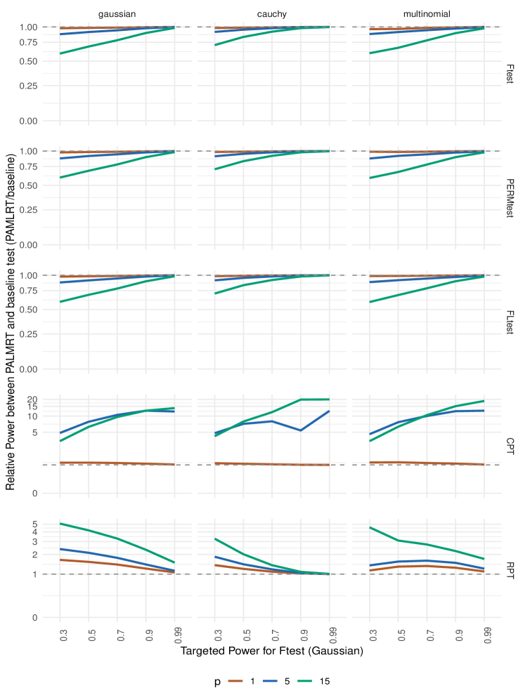
In each experiment, we simulate data from the alternative setting by varying the linear coefficient in front of in eq. (11):
| (11) |
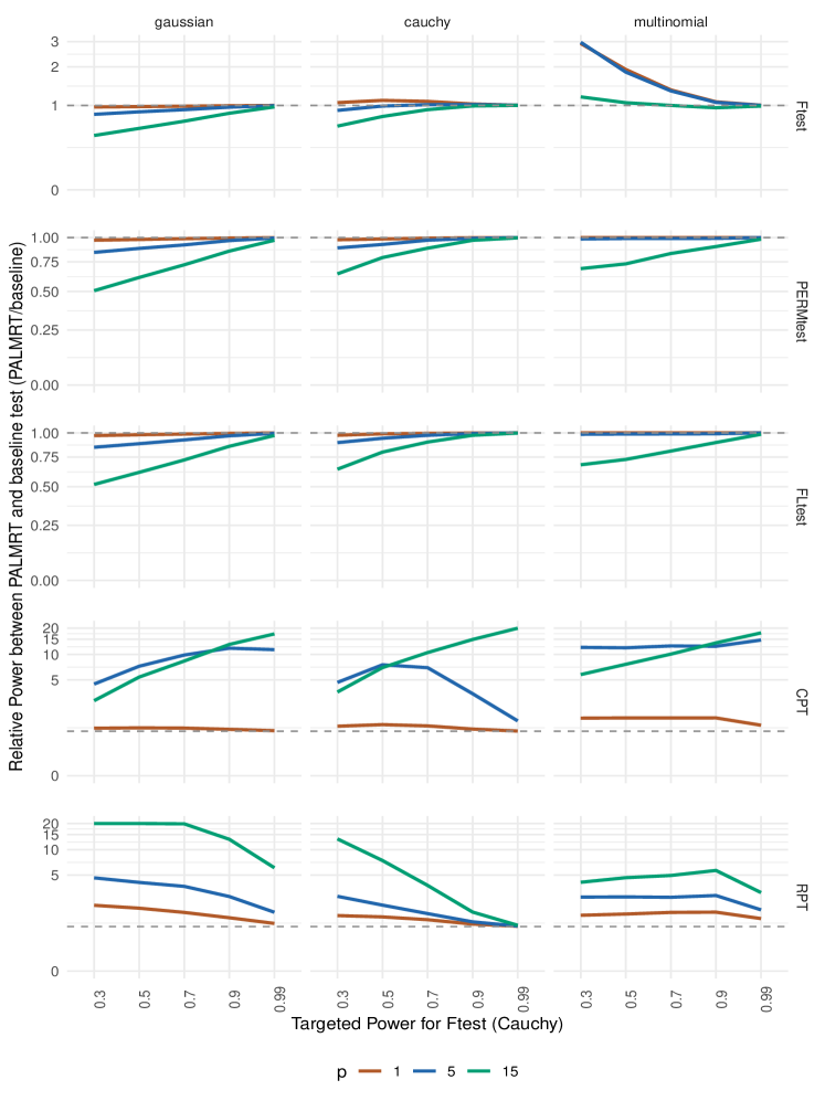
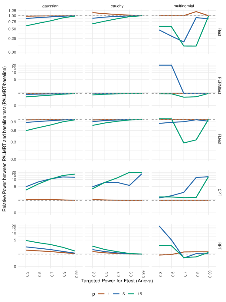
We set using Monte-Carlo simulation to yield F-test powers of approximately , , , , . Figures 3-5 display the median of relative power of PALMRT to F-test, PERMtest, FLtest, CPT and RPT for varying signal strengths, noise distributions and feature dimensions under Gaussian, Cauchy, and ANOVA designs. For visualization purposes, if a median ratio is greater than 20, it is truncated at 20.
Under the Gaussian design, Ftest, PERMtest, and FLtest are most powerful across various noise types and feature dimensions. PALMRT closely rivals them at and its relative sensitivity to low signal strength decreases with increased feature dimensions. PALMRT achieves higher power than CPT at and substantially outperforms CPT at and , despite being more empirically conservative for controlling the type I error. The gap between CPT and PALMRT does not disappear for and as we increase the signal strength. This is very different from the group bound method (Meinshausen, 2015) which is also conservative but is powerless compared to CPT in a wide range of signal-to-noise ratios when examined in Lei and Bickel (2021). PALMRT also shows much higher power compared to RPT with different concomitant feature dimension , especially among the regime with a low signal-to-noise ratio.
In the Cauchy design, the relative sensitivities of PALMRT trend similarly to the Gaussian setting. However, F-test loses power with heavy-tailed noise distributions like Cauchy or multinomial, and random permutation tests can outperform F-test at low signal strengths. In the ANOVA design, results align with the Cauchy design when the noise is Gaussian or Cauchy. When the noise is multinomial, although the overall pattern is difficult to characterize, CPT and RPT are both significantly worse than PALMRT.
Overall, PALMRT has consistently higher power than CPT in the Gaussian, Cauchy, and ANOVA designs, despite becoming more conservative as increases, and is also more powerful than RPT. When is large, PALMRT and FLtest perform similarly, but their relative diverges as decreases. This divergence is contingent on both design and noise distributions.
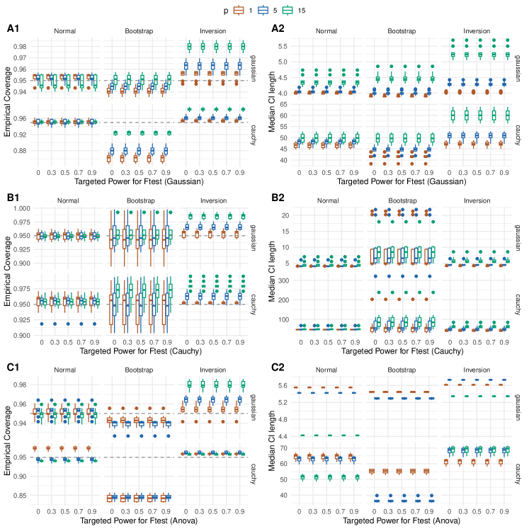
6.3 Coverage evaluation of
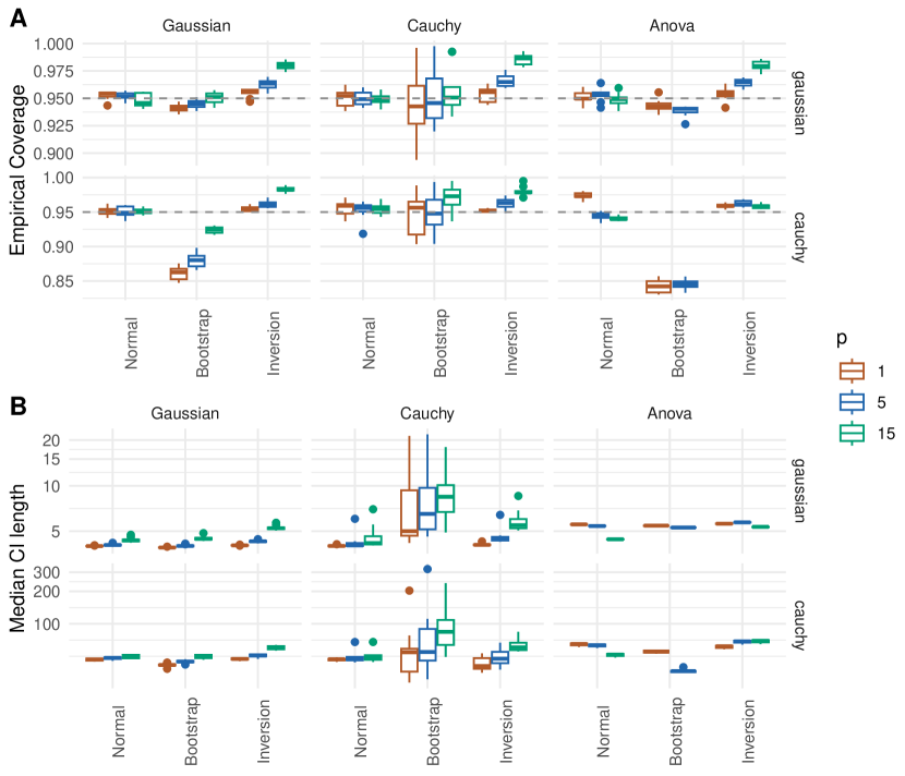
In this section, we evaluate the empirical coverage and median length of confidence intervals () constructed using Algorithm 2 (“Inversion”), Bootstrap, and normal approximation (“Normal”) across Gaussian, Cauchy, and Anova designs for various . We exclude the Paired design due to undefined Bootstrap CIs for all . As CI coverage and length are consistent across different , for the sake of space, we focus on results with a targeted F-test power of and defer full results to the supplementary materials.
Figure 6A presents the achieved coverage. The CIs from Inversion consistently meet the desired coverage. In contrast, the normal CIs exhibit slight under-coverage in the ANOVA design with Cauchy noise, and Bootstrap CIs show severe under-coverage for Cauchy noise. For the ANOVA design with , Bootstrap CIs are undefined and thus omitted in Figure 6A. Figure 6B shows the median CI lengths for each method. In line with previous findings, CIs from Algorithm 2 are generally wider than Normal CIs, except for with Cauchy noise. Bootstrap CIs can exhibit greater variability when the designs are dominated by extreme values, such as in the Cauchy design setting.
7 Robust Identification of long-Covid biomarkers
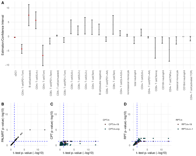
The MY-LC dataset contains measurements of 64 cell frequencies for 101 long-Covid (LC) participants and 84 controls (42 healthy samples, 42 convalescent samples without LC). A small percentage of measures are missing, with the number of observed samples ranging from 169 to 177 across features. Significant partial correlations between LC status and cell frequencies were identified by Klein et al. (2023), after controlling for age, sex, and BMI as described in eq. (2). Among the 64 features, 26 had , and 5 survived multiple hypothesis correction using the BH procedure. In this work, we apply PALMRT, CPT, and RPT, which are theoretically guaranteed and validated through simulations, for robust biomarker identification.
Figure 7A displays confidence intervals generated using Algorithm 2 for the 26 significant biomarkers identified by the t-test, before multiple corrections, at . The center dot in each CI represents the estimated LC coefficient in eq. (2). Solid dots indicate features that were significant before correction; empty dots indicate otherwise. PALMRT confirmed 24 of these 26 biomarkers. In particular, all 5 top biomarkers, which were significant after correction using the t-test, remained significant after correction using PALMRT (solid dot with red circle). In general, the p-values from PALMRT and the t-test are highly concordant, with ratios between them for the same feature ranging from 0.6 to 1.2, except for cDC1 and the central memory CD4+ T cell with positive PD1 (CD4+ T cell (PD1+Tcm)), which achieved the smallest possible PALMRT p-values at and also had smallest t-test p-values (see Figure 7B).
Both CPT and RPT, in contrast, reduced discoveries before correction and yielded none afterward. Increasing the number of cyclic permutations () from to did not improve their power in CPT, as shown in Figure 7C. The nominal p-value cutoff at 0.05 resulted in 16 out of 26 t-test discoveries being confirmed when and none being significant when (see Figure 7C). RPT achieved higher power compared to CPT at the nominal p-value cutoff of 0.05, confirming 22 out of 26 t-test discoveries when . However, even for RPT, no discoveries were retained after correcting for multiple hypothesis tests, whether using or , the largest allowed by the RPT algorithm (see Figure 7D).
8 Discussions
We introduce a novel conformal test, PALMRT, designed for hypothesis testing in linear regression. This test and its corresponding confidence intervals are efficiently computed by evaluating statistic pairs, which are formed by augmenting the original regression problem with row-permuted versions of . PALMRT achieves little power loss compared to conventional tests like the F/t-test and FL-test, and differs from CPT and RPT which also enjoy a worst-case coverage guarantee. Unlike CPT, PALMRT eliminates the need for complex optimization to construct the test and consistently outperforms CPT in both simulated and real-data scenarios. In comparison to RPT, another recently proposed method, developed independently to address the challenges in CPT, PALMRT does not require specially designed permutations that form a group, and its performance remains stable and does not deteriorate as the number of permutations increases.
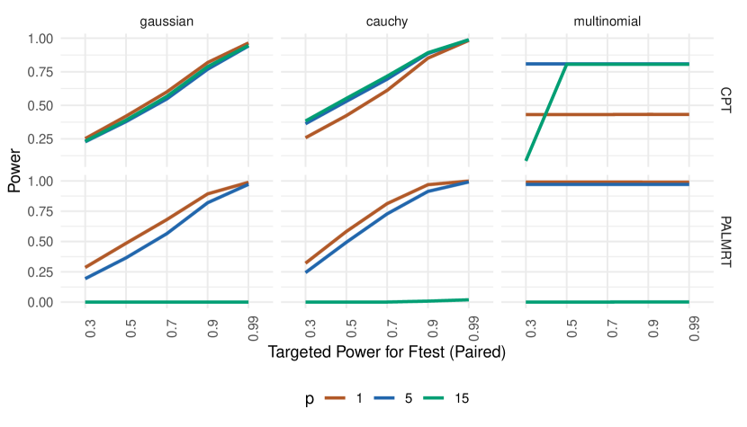
Of note, the improvement over CPT is not universal. For example, in special designs like the paired design where there are many duplicate rows in , CPT can be more powerful. Figure 8 illustrates the comparative power of CPT and PALMRT in signal detection under the paired design. While PALMRT generally matches or exceeds the power of CPT when , it fails to detect signals at when . CPT, conversely, successfully identifies an effective pre-ordering and to construct a non-trivial test. While such settings are rare in practice, this observation raises an intriguing theoretical inquiry: Can the power of PALMRT be enhanced by filtering the random permutations to avoid near co-linearity among ? We earmark this question for future exploration.
As a brief detour from our main discussion, the augmentation step in PALMRT is reminiscent of the seminal work by Barber and Candès (2015), which introduced the concept of knockoffs. This approach generates a knockoff copy of the original feature matrix , e.g., in our notation with dimension . The key requirement of the knockoff copy is that swapping any pair leaves the covariance structure unchanged. Consequently, important quantities in regression analysis—such as OLS or Lasso coefficients —are invariant under these swaps, provided the error terms are i.i.d Gaussian. Knockoffs control the FDR by retaining features for which is sufficiently large. Although both PALMRT and knockoffs operate under a fixed design and have similar sample size requirements, their objectives differ. Knockoffs aim to control FDR across features under the Gaussian noise assumption, often in more complex model-fitting contexts, whereas PALMRT focuses on computing individual p-values for partial correlations under a more relaxed exchangeability condition for the residual errors. Recent advancements in derandomized knockoffs (Ren and Barber, 2022) allow for the computation of modified e-values (Vovk and Wang, 2021; Wang and Ramdas, 2022) through repeated runs with different copies. However, achieving small p-values or high e-values necessitates a large or at least, a constraint not shared by PALMRT. This makes PALMRT particularly advantageous for exploratory analyses aimed at uncovering partial correlations among a potentially large set of response and primary feature pairs, after adjusting for a limited number of covariates.
Acknowledgment
The author would like to thank Dr. Akiko Iwasaki and her team for providing access to the MY-LC data.
Funding
L.G. was supported in part by the NSF award DMS2310836.
References
- Anderson and Robinson (2001) Anderson, M. J. and J. Robinson (2001). Permutation tests for linear models. Australian & New Zealand Journal of Statistics 43(1), 75–88.
- Barber and Candès (2015) Barber, R. F. and E. J. Candès (2015). Controlling the false discovery rate via knockoffs. The Annals of Statistics 43(5).
- Barber et al. (2021) Barber, R. F., E. J. Candes, A. Ramdas, and R. J. Tibshirani (2021). Predictive inference with the jackknife+.
- Davison and Hinkley (1997) Davison, A. C. and D. V. Hinkley (1997). Bootstrap methods and their application. Number 1. Cambridge university press.
- DiCiccio and Efron (1996) DiCiccio, T. J. and B. Efron (1996). Bootstrap confidence intervals. Statistical science 11(3), 189–228.
- Diciccio and Romano (1988) Diciccio, T. J. and J. P. Romano (1988). A review of bootstrap confidence intervals. Journal of the Royal Statistical Society Series B: Statistical Methodology 50(3), 338–354.
- Draper and Stoneman (1966) Draper, N. R. and D. M. Stoneman (1966). Testing for the inclusion of variables in einear regression by a randomisation technique. Technometrics 8(4), 695–699.
- Edgington and Onghena (2007) Edgington, E. and P. Onghena (2007). Randomization tests. CRC press.
- Efron (1987) Efron, B. (1987). Better bootstrap confidence intervals. Journal of the American statistical Association 82(397), 171–185.
- Efron and Narasimhan (2020) Efron, B. and B. Narasimhan (2020). The automatic construction of bootstrap confidence intervals. Journal of Computational and Graphical Statistics 29(3), 608–619.
- Efron and Tibshirani (1994) Efron, B. and R. J. Tibshirani (1994). An introduction to the bootstrap. CRC press.
- Fisher (1922) Fisher, R. A. (1922). The goodness of fit of regression formulae, and the distribution of regression coefficients. Journal of the Royal Statistical Society 85(4), 597–612.
- Fisher (1970) Fisher, R. A. (1970). Statistical methods for research workers. In Breakthroughs in statistics: Methodology and distribution, pp. 66–70. Springer.
- Fisher et al. (1924) Fisher, R. A. et al. (1924). 036: On a distribution yielding the error functions of several well known statistics.
- Freedman and Lane (1983) Freedman, D. and D. Lane (1983). A nonstochastic interpretation of reported significance levels. Journal of Business & Economic Statistics 1(4), 292–298.
- Garthwaite (1996) Garthwaite, P. H. (1996). Confidence intervals from randomization tests. Biometrics, 1387–1393.
- Gupta et al. (2022) Gupta, C., A. K. Kuchibhotla, and A. Ramdas (2022). Nested conformal prediction and quantile out-of-bag ensemble methods. Pattern Recognition 127, 108496.
- Hall (1988) Hall, P. (1988). Theoretical comparison of bootstrap confidence intervals. The Annals of Statistics, 927–953.
- Hall and Wilson (1991) Hall, P. and S. R. Wilson (1991). Two guidelines for bootstrap hypothesis testing. Biometrics, 757–762.
- Han et al. (2023) Han, Y., M. Xu, and L. Guan (2023). Conformalized semi-supervised random forest for classification and abnormality detection. arXiv preprint arXiv:2302.02237.
- Kennedy (1995) Kennedy, F. E. (1995). Randomization tests in econometrics. Journal of Business & Economic Statistics 13(1), 85–94.
- Kim et al. (2020) Kim, B., C. Xu, and R. Barber (2020). Predictive inference is free with the jackknife+-after-bootstrap. Advances in Neural Information Processing Systems 33, 4138–4149.
- Klein et al. (2023) Klein, J., J. Wood, J. Jaycox, R. M. Dhodapkar, P. Lu, J. R. Gehlhausen, A. Tabachnikova, K. Greene, L. Tabacof, A. A. Malik, et al. (2023). Distinguishing features of long covid identified through immune profiling. Nature, 1–3.
- Lei and Bickel (2021) Lei, L. and P. J. Bickel (2021). An assumption-free exact test for fixed-design linear models with exchangeable errors. Biometrika 108(2), 397–412.
- Manly (2006) Manly, B. F. (2006). Randomization, bootstrap and Monte Carlo methods in biology, Volume 70. CRC press.
- Meinshausen (2015) Meinshausen, N. (2015). Group bound: confidence intervals for groups of variables in sparse high dimensional regression without assumptions on the design. Journal of the Royal Statistical Society Series B: Statistical Methodology 77(5), 923–945.
- Pitman (1937) Pitman, E. J. G. (1937). Significance tests which may be applied to samples from any populations. ii. the correlation coefficient test. Supplement to the Journal of the Royal Statistical Society 4(2), 225–232.
- Ren and Barber (2022) Ren, Z. and R. F. Barber (2022). Derandomized knockoffs: leveraging e-values for false discovery rate control. arXiv preprint arXiv:2205.15461.
- Ter Braak (1992) Ter Braak, C. J. (1992). Permutation versus bootstrap significance tests in multiple regression and anova. In Bootstrapping and Related Techniques: Proceedings of an International Conference, Held in Trier, FRG, June 4–8, 1990, pp. 79–85. Springer.
- Vovk et al. (2018) Vovk, V., I. Nouretdinov, V. Manokhin, and A. Gammerman (2018). Cross-conformal predictive distributions. In conformal and probabilistic prediction and applications, pp. 37–51. PMLR.
- Vovk and Wang (2021) Vovk, V. and R. Wang (2021). E-values: Calibration, combination and applications. The Annals of Statistics 49(3), 1736–1754.
- Wang and Ramdas (2022) Wang, R. and A. Ramdas (2022). False discovery rate control with e-values. Journal of the Royal Statistical Society Series B: Statistical Methodology 84(3), 822–852.
- Wen et al. (2022) Wen, K., T. Wang, and Y. Wang (2022). Residual permutation test for high-dimensional regression coefficient testing. arXiv preprint arXiv:2211.16182.
- Westfall and Young (1993) Westfall, P. H. and S. S. Young (1993). Resampling-based multiple testing: Examples and methods for p-value adjustment, Volume 279. John Wiley & Sons.
- Winkler et al. (2014) Winkler, A. M., G. R. Ridgway, M. A. Webster, S. M. Smith, and T. E. Nichols (2014). Permutation inference for the general linear model. Neuroimage 92, 381–397.
Appendix A Proofs
A.1 Proof of Lemma 4.3
Proof.
Recall that and . Hence, does not depend on , and we only need to examine how influences . When lies in the space spanned by , we have , and
Hence, when , we have and when , we have .
When does not lie in the space spanned by , we have, , and
Note that we must have , and consequently, real-valued solutions exist. This follows from the following argument.
Set as the OLS coefficient estimate for in the regression . We have
Here, we use to denote the regression residuals of in the regression . Hence, the previous quadratic function is guaranteed to have real-valued root(s) when . ∎
A.2 Proof of Theorem 4.4
Utilizing Lemma 4.3, we know that value satisfies if and only if
where , , and ; for . We can rearrange for :
| (12) |
Summing over all terms , we obtain that
| (13) |
The function is a piece-wise constant function with change points being . Hence, when , is guaranteed.
When , we must have in order to have since for and . It is obvious that for , . Suppose we know . Then,
-
•
Increasing from to a value in : For all , because for those , smaller than or those no smaller than , their contributions will not change in eq. (13), and only those at exactly at will add contribution or as the corresponding comparisons to change from equality to inequality. Hence, we have
We denote this function value as to indicate being in the open interval .
-
•
Increasing from a value in to : For those , no greater than or those greater than , their contributions will not change in eq. (13), and only those who now hit exactly will add contribution or for newly satisfied comparisons to . Hence, we have
These confirms our induction rule described in the main paper. Finally,
-
•
The smallest value of at the critical values that satisfies is . The smallest interval that satisfies for is , which leads to infimum value . Hence, .
-
•
The largest value of at the critical values that satisfies is . The largest interval that satisfies for is , which leads to supremum value . Hence, .
This conclude our proof that Algorithm 2 constructs the exact described in Lemma 4.3.
Appendix B Additional simulation results
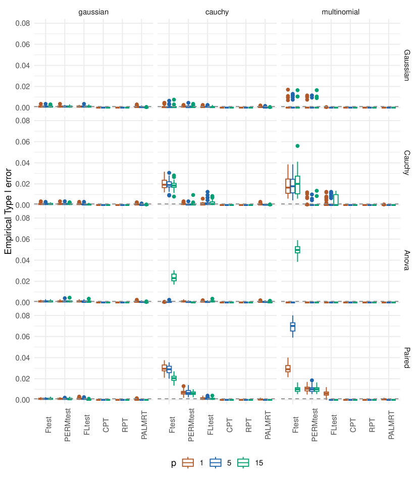
B.1 Type I error control at
.
B.2 CI coverage with varying signal sizes
.