Invariant-based control of quantum many-body systems across critical points

Abstract

Quantum many-body systems are emerging as key elements in the quest for quantum-based technologies and in the study of fundamental physics. In this context, finding control protocols that allow for fast and high fidelity evolutions across quantum phase transitions is of particular interest. Ideally, such controls should be scalable with the system size and not require controllable and unwanted extra interactions. In addition, its performance should be robust against potential imperfections. Here we design an invariant-based control technique that ensures perfect adiabatic-like evolution in the lowest energy subspace of the many-body system, and is able to meet all these requirements – tuning the controllable parameter according to the analytical control results in high-fidelity evolutions operating close to the speed limit, valid for any number particles. As such, Kibble-Zurek scaling laws break down, leading to tunable and much better time scaling behavior. We illustrate our findings by means of detailed numerical simulations in the transverse-field Ising and long-range Kitaev models and demonstrate the robustness against noisy controls and disorder.

Introduction.— Quantum many-body systems are drawing growing interest in modern science, in part, thanks to their great significance in the quest towards scalable quantum-based technological applications, such as in quantum simulation [1, 2], computation [3, 4] and metrology [5, 6, 7]. A precise understanding of quantum many-body physics has also been proven crucial in other research areas, such as material science and statistical mechanics [8, 9, 10]. These systems feature a unique hallmark, namely, the combination of multipartite quantum correlations [11, 12, 13] with collective and emergent phenomena [9, 10]. Due to the limited number of exactly solvable models [14], their understanding usually relies on numerical approaches [15, 16]. Moreover, their complexity and exponentially large Hilbert space pose severe limits to their classical simulations [17]. For these reasons, controllable quantum many-body systems embody a fascinating testbed to develop and test future quantum applications as well as to explore new physics [18, 19, 20].

Quantum phase transitions (QPTs) appear as a genuine trait of quantum many-body systems [21, 22], where fluctuations of quantum nature, rather than thermal, may trigger an abrupt change in the properties of a system in its ground state. This occurs at a certain critical value of an external and controllable parameter, i.e. at the critical point, where relevant quantities display singular behavior, captured by critical exponents [21]. The energy gap typically vanishes at the critical point. Hence, QPTs have profound consequences in both in- and out-of-equilibrium dynamics [18, 19], such as in defect formation described by the celebrated Kibble-Zurek (KZ) mechanism [23, 24, 25, 26, 27, 28, 29, 30]. Based on simple assumptions, the KZ mechanism successfully predicts a universal scaling relation between the density of excitations, the equilibrium critical exponents of the QPT, and the rate at which the critical point is traversed [26], even in the presence of decoherence effects [31, 32]. Such predictions have been experimentally confirmed in a variety of platforms, obeying classical or quantum dynamics [33, 34, 35, 36, 37, 38, 39, 40, 41]. Remarkably, KZ mechanism shows that non-adiabatic excitations are mainly promoted around a QPT where the adiabatic condition unavoidably breaks. This indicates that QPTs pose a great challenge to- and may disrupt the execution of- quantum adiabatic computation or annealing schedules [27, 42, 43] and quantum state preparation in many-body systems [44]. Protocols that allow for a fast and robust evolution through QPTs while providing good fidelities with respect to a target are therefore highly valuable.

Different control techniques have been proposed to speed up an adiabatic evolution, and thus overcome or minimize the loss of adiabaticity caused by a QPT. Ideally, we would demand that the control i) allows for a fast and very high or unit fidelity evolution, ii) does not require further tunability of the system (i.e. extra and specifically tailored interaction terms that must be controlled), iii) presents good scalability with the system size, and iv) is robust against potential imperfections. On the one hand, we find variational quantum controls, such as Krotov [45, 46], machine-learning [47, 48, 49], gradient-based [50, 51] and chopped-random basis quantum optimization [52, 53, 54, 55, 56] protocols. Although they may satisfy i), ii), and iv), the application of these methods to critical systems with many degrees of freedom soon becomes intractable due to the growing number of parameters to be optimized in the cost function. On the other hand, we find shortcuts-to-adiabaticity protocols [57, 58], such as counterdiabatic driving (CD) [59]. Contrary to variational methods, these protocols typically grant unit fidelity by construction at the expense of requiring Hamiltonian diagonalization. As an example, CD can indeed guarantee a perfect-adiabatic-like evolution for any evolution time even when a QPT is traversed, as demonstrated in [60, 61]. Howeve, CD demands an added controllable and time-dependent non-local interaction term, which may be troublesome for its experimental implementation, thus challenging criterion ii). Alternative shortcuts such as those based on invariants of motion [62] still remain challenging due to the lack of dynamical invariants for many-body systems and the challenge of reverse engineering its dynamics. Different protocols have also been proposed, such as local adiabatic [63, 64], fast-quasiadiabatic (FAQUAD) [65] and minimal-action based protocols [66]. It is worth mentioning a recent method based on an optimized CD [67], whose application to quantum many-body systems allows for a significant improvement of both time and fidelity with respect to standard quantum optimal controls, without requiring full knowledge of the system. Nevertheless, such a procedure still demands numerical optimization of a growing number of parameters for larger system sizes and further tunability. Hence, these previously proposed protocols do not meet all the conditions simultaneously.

In this article, we propose a control method for quantum many-body systems that satisfies all the mentioned requirements, i.e. it greatly reduces non-adiabatic excitations even across QPTs, factually leading to error-free evolutions, while operating close to the quantum speed limit. Importantly, the protocol preserves the Hamiltonian in its original form, i.e. without requiring extra interaction or control terms, and it is thus amenable to its experimental realization. The method is precisely based on an invariant control [68], applied to the low-energy subspace of the full Hamiltonian. By construction, the dynamics within the low-energy subspace remain perfectly adiabatic at the end of the passage, so that the resulting excitations stem from transitions between ground- and higher-order excited states. As a consequence, KZ mechanism breaks down: the reduced non-adiabatic excitations no longer depend on the critical exponents and display a much better and tunable scaling with the evolution time. The derived control can be applied to any system size $N$ in a straightforward manner, leading to similar results in terms of a rescaled evolution time. The performance of this invariant-based control is tested in the one-dimensional transverse-field Ising model (TFIM) [21, 69, 22] and long-range Kitaev (LRK) model [70, 71, 72, 73, 74] resulting in analytical controls. The obtained results demonstrate a large improvement over standard methods such as a naive linear ramp and FAQUAD, and corroborate the independence on the universality class, that is, similar results regardless of the critical exponents. Finally, the protocol is shown to be robust against imperfections, such as disorder and noisy controls, while possible future directions are also discussed.

Quantum many-body systems.— We consider two quantum many-body systems where we will illustrate the invariant-based protocol: a TFIM and a LRK [21, 69, 22, 70, 71, 72, 73, 74]. Their Hamiltonians can be written as ($\hbar=1$)

$$\hat{H}_{\rm TFIM} =-J\sum_{i=1}^{N}(g\hat{\sigma}_{i}^{x}+\hat{\sigma}_{i}^{z}\hat{\sigma}_{i+1}^{z}),$$ (1)

$$\hat{H}_{\rm LRK} =-J\sum_{i=1}^{N}\left[\sum_{r>0}(J_{r}\hat{c}_{i}^{\dagger}\hat{c}_{i+r}+d_{r}\hat{c}_{i}\hat{c}_{i+r}+{\rm H.c.})-g\hat{n}_{i}\right],$$ (2)

where $\hat{\sigma}_{i}^{x,y,z}$ denote the spin-$1/2$ matrices at site $i$, while $\hat{c}_{i}$ corresponds to fermionic annihilation operator, and $\hat{n}_{i}=\hat{c}_{i}^{\dagger}\hat{c}_{i}$. In both cases $J$ accounts for an energy scale for the $N$ interacting particles separated by a distance $a$, while $g$ is a dimensionless controllable parameter, which in the TFIM represents the magnetic-field strength and in the LRK the chemical potential. Periodic boundary conditions are taken for both models. These models feature continuous QPTs at a certain critical value $g_{c}$ of this external parameter $g$. For the TFIM, $g_{c}=1$. In the LRK, hopping and pairing strengths, $J_{r}$ and $d_{r}$, respectively, depend on long-range exponents $\alpha,\beta>1$, that is, $J_{r}=(N_{\alpha}r^{\alpha})^{-1}$ and $d_{r}=(N_{\beta}r^{\beta})^{-1}$ with $N_{\gamma}=2\sum_{r=1}^{N/2}r^{-\gamma}$ for $\gamma=\{\beta,\alpha\}$ following Kac’s prescription [75]. Thus, critical properties of the LRK also depend on $\alpha$ and $\beta$. In the short-range limit, $\alpha,\beta\rightarrow\infty$, the critical point takes place at $g_{c}=2J$, and the model maps to a TFIM [70].

Both Hamiltonians can be decoupled into a collection of independent Landau-Zener systems in momentum space of spinless fermions, which greatly simplifies the dynamics. The full Hamiltonian can be diagonalized as $\hat{H}=\sum_{k}\Psi^{\dagger}_{k}\hat{H}_{k}\Psi_{k}$, with $\Psi^{\dagger}=(\hat{c}_{k}^{\dagger},\hat{c}_{-k})$, where $\hat{c}_{k}^{\dagger}$ is the creation operator of a spinless fermion with momentum $k$. In this momentum space, one can write $\hat{H}_{k}=h_{z,k}(g)\hat{\sigma}_{z}^{k}/2+h_{x,k}\hat{\sigma}_{x}^{k}/2$, such that $\hat{\sigma}_{z}^{k}=\ket{1}\bra{1}_{k}-\ket{0}\bra{0}_{k}$ represents the $z$-component of the Pauli matrices for the quasiparticles of momentum $k=(2n-1)\pi/Na$ with $a$ the interparticle distance, and $n\in\{1,\ldots,N/2\}$ (see for example [21, 71]). For the TFIM, $h_{z,k}(g)=4J(g-\cos(ka))$, $h_{x,k}=4J\sin(ka)$, while for the LRK, $h_{z,k}(g)=g-4J\sum_{r>0}J_{r}\cos(kra)$ and $h_{x,k}=-2J\sum_{r>0}d_{r}\sin(kra)$. The minimum energy gap takes place at the QPT, at $g_{c}$. In the thermodynamic limit, $N\rightarrow\infty$, one finds $\Delta(g)\propto|g-g_{c}|^{z\nu}$ with $z\nu=1$ (TFIM), while $z$ and $\nu$ depend on the range of the interactions in the LRK [74].

Our goal consists in devising controls $g\equiv g(t)$ that drive an initial ground state in one phase, $\ket{\psi(t=0)}=\ket{\phi_{0}(g_{0})}$ with $g_{0}>g_{c}$, into the ground state in the other phase across the QPT ($g_{1}<g_{c})$, namely, $\ket{\psi(\tau)}=\ket{\phi_{0}(g_{1})}$ where $\ket{\psi(\tau)}=\mathcal{U}(\tau,0)\ket{\psi(0)}$ and $\mathcal{U}(t_{1},t_{0})=\mathcal{T}e^{-i\int_{t_{0}}^{t_{1}}dt^{\prime}H(t^{\prime})}$ the time-evolution operator. Since $\langle\phi_{0}(g_{0})|\phi_{0}(g_{1})\rangle\approx 0$, the minimum time to perform this evolution, known as quantum speed limit (QSL), amounts to $\tau_{\rm QSL}=\pi/\Delta$ with $\Delta$ the minimum energy gap throughout the evolution [76].

Invariant-based control.— In the following we discuss how to construct the time-dependent protocol $g(t)$ based on a invariant control of the low-energy subspace of a many-body system. For that, we start from the most general low-energy Hamiltonian, $\hat{H}(t)=\frac{1}{2}\sum_{a}h_{a}(t)\hat{\sigma}_{a}$ with $[\hat{\sigma}_{b},\hat{\sigma}_{c}]=2i\epsilon_{abc}\hat{\sigma}_{a}$ where $\epsilon_{abc}$ is the antisymmetric Levi-Civita tensor, with $a,b,c\in\{x,y,z\}$. By a proper design of the controls time-dependency it is in general possible to connect two different states on the Bloch sphere irrespective of the process invested time $\tau$. Associated with the Hamiltonian there are time-dependent Hermitian invariants of motion in the Schrödinger picture $\hat{I}(t)$ satisfying

$$\frac{d\hat{I}}{dt}\equiv\frac{\partial\hat{I}(t)}{\partial t}+i[\hat{H}(t),\hat{I}(t)]=0.$$ (3)

It can be shown [77] that a wavefunction $\ket{\psi(t)}$ which evolves with $\hat{H}(t)$ can be expanded as a linear combination of invariant modes $\ket{\psi(t)}=\sum_{j}c_{j}e^{i\alpha_{j}}\ket{\varphi_{j}(t)}$ with $c_{j}$ constant expansion coefficients, $\alpha_{j}$ the Lewis-Riesenfeld phases, and the invariant eigenvectors assumed to form a complete set $\hat{I}(t)\ket{\varphi_{j}(t)}=\lambda_{j}\ket{\varphi_{j}(t)}$ with $\lambda_{j}$ being the constant eigenvalues. Note that the previous expansion sets the dynamical wave function to evolve along the instantaneous superposition of eigenstates of $\hat{I}(t)$, while excited states of $\hat{H}(t)$ are allowed to be populated during the dynamics, in contrast to an adiabatic passage. Codifying the initial and target states in the ground states of the boundary Hamiltonians $\hat{H}(t_{B})$ with $t_{B}=0,\tau$, the two states are perfectly connected by reverse engineering the dynamics, i.e. imposing the time-dependency of the invariant through the frictionless conditions $[\hat{H}(t_{B}),\hat{I}(t_{B})]=0$ to ensure a perfect driving (such that the initial and final states become eigenstates of both $\hat{H}$ and $\hat{I}$) and then deducing the Hamiltonian controls $h_{i}(t)$. An invariant for a two-level system can be constructed as $\hat{I}(t)=\frac{1}{2}\sum_{a}f_{a}(t)\hat{\sigma}_{a}$, with $f_{a}(t)$ arbitrary time-dependent functions fulfilling Eq. (3). This forms a set of coupled differential equations that can be inverted if $\sum_{a}f_{a}^{2}=K$ with $K$ a constant, leading to the Hamiltonian controls in terms of the invariant $f_{a}(t)$ free-functions [78]

$$h_{a}=\frac{1}{f_{c}}\big{(}f_{a}h_{c}-\epsilon_{abc}\dot{f}_{b}\big{)},$$ (4)

with all indices $a,b,c$ different and $h_{y}(t)=0$ chosen for convenience to avoid a $\hat{\sigma}_{y}$ interaction in $\hat{H}(t)$. After extrapolation of the invariant free functions fulfilling the frictionless conditions $f_{a}(t_{B})h_{b}(t_{B})-f_{b}(t_{B})h_{a}(t_{B})=0$ with $a\neq b$, an infinite family of Hamiltonian controls is deduced from (4) such that the time dependency ensures a perfect driving connecting the desired initial and target states of the low-energy subsystem.

The previous derivation can be readily applied to the TFIM and LRK models to control the lowest subspace with momentum $k_{0}$. Indeed, using (4) we arrive at $h_{z,k_{0}}(g)=(\ddot{f}_{z}+f_{z}h_{x,k_{0}}^{2})/(h_{x,k_{0}}(K-f_{z}^{2}-\dot{f}_{z}^{2}/h_{x,k_{0}}^{2})^{1/2})$, from where the control $g(t)$ can be analytically determined [78]. As an illustration, the control $g(t)$ for a TFIM with $N=200$ spins employing a fifth-order polynomial for $f_{z}$ is plotted in Fig. 1(a). The minimum evolution time for this choice results in $\tau\gtrsim 1.2\tau_{\rm QSL}$ [78].

Breakdown of Kibble-Zurek mechanism and quasiadiabatic dynamics.— Critical features of the QPT typically leave their footprint on the dynamics. The KZ mechanism [27, 26] predicts an unavoidable departure from an adiabatic evolution due to a vanishing energy gap $\Delta(g)\propto|g-g_{c}|^{z\nu}$. This adiabatic-impulse approximation in the vicinity of the QPT leads to the celebrated KZ scaling relations, such as the density of excitations $n\sim\tau^{-d\nu/(z\nu+1)}$ for a linear ramp across the QPT with $\dot{g}\propto 1/\tau$, and $d$ being the spatial dimension of the system [27, 26, 43, 18]. Here $n=1-\frac{2}{N}\sum_{k>0}|\langle\phi_{k,0}|\psi_{k}(\tau)\rangle|^{2}$ with $\ket{\phi_{k,0}}$ the ground state at $g(\tau)$ in the $k$ subspace, and $\ket{\psi_{k}(\tau)}$ the evolved state. However, an engineered control $g(t)$ that strictly ensures an adiabatic-like evolution within the lowest-energy subspace will not follow KZ mechanism. Under this $g(t)$, the system evolves as being gapped throughout the whole quench, i.e. as it had no critical or singular traits . This results in the breakdown of the KZ mechanism, i.e. $n\sim\tau^{-dv/(z\nu+1)}$ will no longer be applicable.

The invariant-based control $g(t)$ ensures adiabaticity at the end of the passage in the lowest subspace. The dynamics within higher-order subspaces may be quasi-adiabatic due to their larger energy separation. The resulting time scaling, different from KZ prediction, can be obtained by relying on a simple Landau-Zener system. Its Hamiltonian, with minimum energy gap $\Delta_{1}$, is quenched from its ground state following a control $g(t)$. The control $g(t)$ is determined by Eq. (4) and its boundary conditions so that it ensures the target adiabatic state in a subspace with gap $\Delta_{0}<\Delta_{1}$. Applying adiabatic perturbation theory [80], one can show that [78] the density of excitations $n$ scales as $n\propto|\dot{g}(t_{B})|^{2}$, and similarly infidelity $\mathcal{I}=1-\mathcal{F}$ with $\mathcal{F}=\langle\phi_{0}(g_{1})|\psi(\tau)\rangle|^{2}$ [78]. For linear ramps, $\dot{g}(t_{B})\propto\tau^{-1}$ resulting in the standard $\tau^{-2}$ time scaling for quasi-adiabatic dynamics. In our case, however, $\dot{g}(t)$ depends on the auxiliary function $f_{z}$. Choosing a polynomial, $\dot{g}(t_{B})\propto\dddot{f_{z}}(t_{B})$ since $\dot{f}_{z}(t_{B})=\ddot{f}_{z}(t_{B})=0$ by construction [78], as well as $\dddot{f}_{z}(t_{B})\propto\tau^{-3}$, we have $n\sim\tau^{-6}$. This scaling can be further improved by noticing that the auxiliary function $f_{z}$ is arbitrary, and can be constructed requiring all first $k-1$ time-derivatives of $f_{z}$ to vanish at the boundaries $t_{B}$. In this manner, one finds

$$n\propto|d^{k}f_{z}(t_{B})/dt^{k}|^{2}\propto\tau^{-2k},$$ (5)

for $k\geq 3$, so that the time-scaling across QPTs can be arbitrarily enhanced.

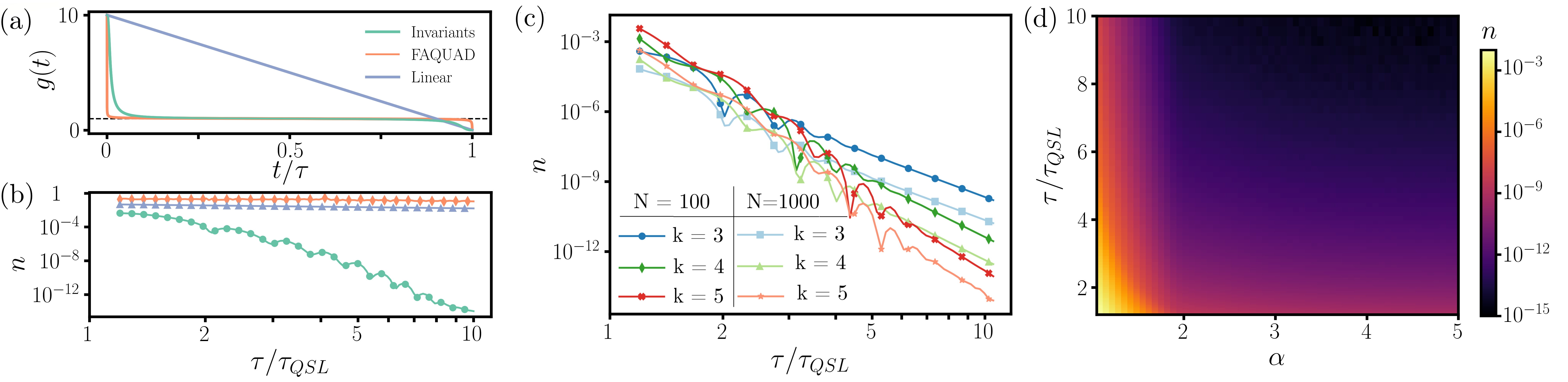
Figure 1: (a) Sketch of the invariant, FAQUAD, and linear controls starting at $g(0)=10$ and ending at $g(\tau)=0$, simulated for $N=200$ spins. (b) Scaling of the density of excitations (log-log) for the TFIM and fixed $N=200$ spins for the three protocols. (c) TFIM invariant for $N=100$ and $N=1000$ as a function of the rescaled quench time $\tau/\tau_{\rm QSL}$, Including also the $\tau^{-8}$ and $\tau^{-10}$ protocols. (d) Scaling of $n$ in the LRK for $N=100$ fermions, $\beta\rightarrow\infty$, as a function of the quench time $\tau$ (in units of $\tau_{\rm QSL}$) and the long-range exponent $\alpha$.

Numerical results.— These theoretical predictions are corroborated by numerical simulations in the TFIM and LRK for different long-range exponents. For completeness, we compare the invariant-based control with a linear ramp and FAQUAD designed for the low-energy subspace. The results for the density of excitations $n$ for a TFIM with $N=200$ spins, $g(0)=10$ and $g(\tau)=0$, are plotted in Fig. 1(b), which reveal an improvement of the invariant control by several orders of magnitude with respect to these other protocols, and clearly breaking the KZ scaling law. Note that already for $\tau\approx 2\tau_{\rm QSL}$, we obtain $n\sim 10^{-5}$, improving by 4 orders of magnitude at $\tau\approx 5\tau_{\rm QSL}$. In addition, the time scaling agrees with the $\tau^{-2k}$ law independently on the system’s size, as shown in Fig. 1(c) for $k=3$, $4$ and $5$ with a suitably chosen $f_{z}$ [78]. Similar results are obtained for the infidelity. The resulting dynamics are agnostic to the critical features, as shown for the LRK with different long-range exponent (cf. Fig. 1(d)). However, extremely long-ranged interactions may cause gapless higher-excited states at the critical point, such as in mean-field models. This makes the derived control unfit to provide speedup adiabatic evolutions for $\alpha\rightarrow 1$ in the LRK.

Robustness.— Having shown that the invariant-based control fulfill the requirements i), ii), and iii) mentioned in the introduction, namely, high fidelities for fast evolutions, minimal tunability, and good scalability with the system size, we bring our attention to the iv) criterion. That is, its robustness against potential imperfections. For that, we analyze the performance of the invariant-based protocol designed for an ideal TFIM under noisy control as well as under random disorder. First, we consider a $\hat{H}_{\rm TFIM}$ with $g(t)\rightarrow g(t)+\eta(t)$ (cf. Eq. (1)), being $\eta(t)$ a white Gaussian noise that accounts for fluctuations on the control, so that $\langle\eta(t)\rangle=0$ and $\langle\eta(t)\eta(t^{\prime})\rangle=W^{2}$, with $W$ the strength of the fluctuations. The dynamics, in this case, can be calculated exactly [31, 78], leading to a master equation in Lindblad form for each subspace, $\dot{\hat{\rho}}_{k}=-i[\hat{H}_{0,k}(t),\hat{\rho}_{k}(t)]+\mathcal{D}_{1,k}[\hat{\rho}_{k}(t)]$. The incoherent part is given by $\mathcal{D}_{1,k}[\hat{\rho}_{k}]=\Gamma(\hat{L}_{k}\hat{\rho}_{k}\hat{L}_{k}^{\dagger}-\frac{1}{2}\{\hat{L}_{k}^{\dagger}\hat{L}_{k},\hat{\rho}_{k}\})$ with $\Gamma=4J^{2}W^{2}$ and $\hat{L}_{k}=\hat{\sigma}_{z}^{k}$ [78].

The results are gathered in Fig. 2(a) where we show the density of excitations $n$ as a function of the quench time $\tau$ for $N=50$ spins for different noise strengths $W$. As it can be seen, the invariant-based control performs well even for moderate values of $W$, still revealing its characteristic $\tau^{-2k}$ scaling with $k=3$. Its performance is better illustrated in the inset of Fig. 2(a), where $n$ is plotted against $W$ for two quench times, namely, $\tau/\tau_{\rm QSL}=2$ and $\tau/\tau_{\rm QSL}=5$. Similar results are obtained for larger system sizes. Recall that the critical exponents are irrelevant for the scaling properties, and thus no universal anti-KZ scaling can be found under this protocol (see however Refs. [31, 32]).

We also examine the impact of interaction-strength disorder. We consider dimensionless, independent and identically distributed uniform random variables $\lambda_{i}\in[1-\Lambda,1+\Lambda]$, so that $\hat{H}_{\rm TFIM}=-J(g\sum_{i=1}^{N}\hat{\sigma}_{i}^{x}+\sum_{i=1}^{N}\lambda_{i}\hat{\sigma}_{i}^{z}\hat{\sigma}_{i+1}^{z})$ [81, 82, 83]. The ideal case considered above is recovered for $\Lambda=0$ (cf. Fig. 1 and Eq. (1)). The dynamics are solved for different disorder realizations $\{\lambda_{i}\}$, and then averaging the obtained results (see [78] for details). The averaged $n$ as a function of $\Lambda$ is plotted in Fig. 2(b) for $N=50$ spins. The ideal result is achieved for $\Lambda=0$, while even for a non-negligible disorder, e.g. $\Lambda\approx 0.2$, and close to $\tau_{\rm QSL}$ the density of excitations can be found below $10^{-3}$. As for the noisy control, the invariant-based control designed for the ideal TFIM results in robust and highly adiabatic-like evolutions operating close to the quantum speed limit.

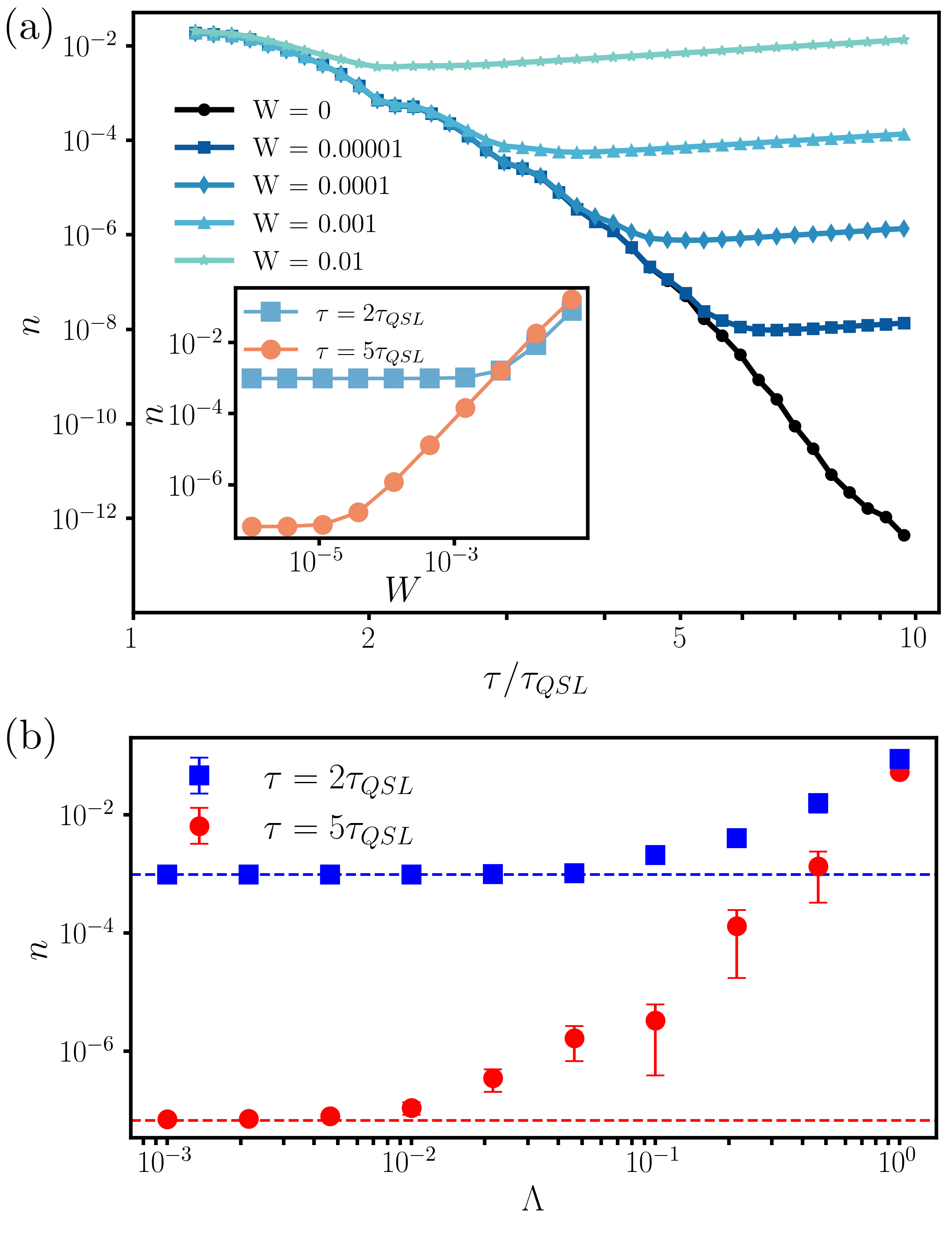
Figure 2: Robustness for noisy control. (a) The density of excitations as a function of the rescaled quench time, for $N=50$ spins and for different white Gaussian noise strengths $W$ affecting the control. (b) Impact of local random disorder $\lambda_{i}$ in the average density of excitations (after $10$ repetitions) as a function of the disorder strength $\Lambda$ for $N=50$ spins, $g(0)=10$ and $g(\tau)=0$. Error bars correspond to a standard deviation, while dashed lines represent the ideal $\Lambda=0$ case. See main text for details.

Conclusions.— In this work we have obtained families of protocols to control quantum many-body systems across QPTs providing high-fidelity evolutions and operating close to the quantum speed limit. The method is based on an invariant control of the low-energy subspace of the many-body system. Our proposed protocol does not require the addition of extra terms in the Hamiltonian, as is the case for counterdiabatic driving, and just requires a particular time-dependent shape of the controllable external parameter, thus making it amenable for its experimental realization. This is illustrated in two relevant models (TFIM and LRK), where we work out analytical expressions for the time-dependent control for any system size. By construction, the resulting dynamics are agnostic to the critical features of the QPT, and therefore, KZ mechanism breaks down, leading to much better time scalings. The robustness of the invariant-based method is studied against two distinct sources of imperfections, noisy control, and disorder in the interaction’s strengths. The proposed method can be readily applied to current experimental setups, with application in quantum adiabatic computation and state preparation. An interesting direction for future investigations consists in extending these protocols to generic non-integrable many-body systems.

Supplemental Material
Invariant-based control of quantum many-body systems across critical points

Hilario Espinós Loris Maria Cangemi Amikam Levy Ricardo Puebla Erik Torrontegui

I A. Fast quasi-adiabatic dynamics

We are interested in the control of the Hamiltonian

$$\hat{H}(t)=h_{x}\frac{\hat{\sigma}_{x}}{2}+h_{z}(t)\frac{\hat{\sigma}_{z}}{2},$$ (S1)

such that the initial ground state $|-(0)\rangle$ of $\hat{H}(0)$ with $h_{z}(0)=h_{z}^{0}$ is evolved in a time $\tau$ to the target final state that corresponds to the ground state $|-(\tau)\rangle$ of $\hat{H}(\tau)$ with $h_{z}(\tau)=h_{z}^{F}$. Note that the control $h_{x}(t)=h_{x}$ is time independent and $h_{y}(t)=0$ $\forall t$. The instantaneous eigenvectors of the Hamiltonian are given by

$$\ket{+(t)}=\cos{\frac{\theta}{2}}\ket{0}+\sin{\frac{\theta}{2}}\ket{1},$$

$$\ket{-(t)}=\sin{\frac{\theta}{2}}\ket{0}-\cos{\frac{\theta}{2}}\ket{1},$$ (S2)

with $\ket{0}$ and $\ket{1}$ being the eigenstates of $\hat{\sigma}_{z}$ and $\tan{\theta}=h_{x}/h_{z}(t)$. The corresponding eigenenergies $E_{\pm}(t)=\pm\frac{1}{2}\sqrt{h_{x}^{2}+h_{z}(t)^{2}}$ are depicted in Fig. S1(a) showing an avoided crossing $\Delta E=E_{+}-E_{-}$ with a minimum gap $\Delta E_{\rm min}=h_{x}$ at $h_{z}(t)=0$. The Hamiltonian exhibits a typical Landau-Zener passage when the rate of change of the gap $\Delta E$ is slow compared to the intrinsic dynamics of the system

$$\mu(t)=\bigg{|}\frac{\braket{-(t)}{\partial_{t}+(t)}}{E_{-}(t)-E_{+}(t)}\bigg{|}=\bigg{|}\frac{\bra{-(t)}\frac{\partial\hat{H}}{\partial t}\ket{+(t)}}{[E_{-}(t)-E_{+}(t)]^{2}}\bigg{|}=\bigg{|}\frac{h_{x}\dot{h}_{z}(t)}{2[h_{x}^{2}+h_{z}^{2}(t)]^{3/2}}\bigg{|}\ll 1\quad\forall t.$$ (S3)

In case of such adiabatic evolution, the state of the system follows the instantaneous eigenstates (I) up to a global phase. Equation (S3) is the condition for an adiabatic driving at the expense of a global constraint on the control change rate, during the whole process, to its minimum value, $\Delta E_{\rm min}$, leading to slow passages.

The fast quasi-adiabatic dynamics formalism [65] aims at preserving the adiabatic condition locally in time. This can be done by making the adiabaticity parameter constant $\mu(t)=c_{\mu}\ll 1$ such that the transition probability is equally delocalized during the whole process. Integrating $\mu(t)=c_{\mu}$ with the initial and final conditions $h_{z}(0)=h_{z}^{0}$ and $h_{z}(\tau)=h_{z}^{F}$ sets a value for the integration constant and the adiabaticity parameter $c_{\mu}$ leading to a lengthy but analytical control. Its shape is depicted in Fig. S1(b), as shown, the derived $h_{z}(t)$ allows fast variations when the avoided crossing opens and remains constant in the proximity to $\Delta E_{\rm min}$.

II B. Invariant-based control

The starting point is the Hamiltonian (S1) with the same boundary conditions, i.e., $h_{z}(0)=h_{z}^{0}$ and $h_{z}(\tau)=h_{z}^{F}$ at the final time $\tau$, while during the whole evolution $h_{x}(t)=h_{x}=const$ and $h_{y}(t)=0$. To reverse engineer the control Hamiltonian $H(t)$, we note that it is constructed from the Pauli matrices which are the generators of the SU(2) Lie algebra,

$$[\hat{\sigma}_{b},\hat{\sigma}_{c}]=2i\epsilon_{abc}\hat{\sigma}_{a},$$ (S4)

with $\epsilon_{abc}$ the anti-symmetric Levi-Civitta tensor. Associated with the Hamiltonian there are time-dependent Hermitian invariants of motion $\hat{I}(t)$ that satisfy

$$\frac{d\hat{I}}{dt}\equiv\frac{\partial\hat{I}(t)}{\partial t}-\frac{1}{i}[\hat{H}(t),\hat{I}(t)]=0.$$ (S5)

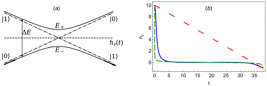
Figure S1: (a) Landau-Zener passage through the avoided crossing of Hamiltonian (S1). (b) Different shapes of the $h_{z}$ driving, invariant-based (blue-solid line), FAQUAD (green-dashed line), and linear (red-dotted line) as a function of $t$ for the minimum ramp time $\tau=38$ of Fig. S2. Parameter values: $h_{z}(0)=10$, $h_{z}(\tau)=-1$, and $h_{x}=0.1$.

A dynamical wave function $|\Psi(t)\rangle$ which evolves with $\hat{H}(t)$ can be expressed as a linear combination of invariant modes

$$|\psi(t)\rangle=\sum_{j}c_{j}e^{i\alpha_{j}}|\phi_{j}(t)\rangle,$$ (S6)

where the $c_{j}$ are constants, and the phases $\alpha_{j}$ fulfill

$$\frac{d\alpha_{j}}{dt}=\langle\phi_{j}(t)|i\frac{\partial}{\partial t}-\hat{H}(t)|\phi_{j}(t)\rangle,$$ (S7)

and the eigenvectors of $\hat{I}(t)$, $|\phi_{j}(t)\rangle$ forms a complete set that satisfies

$$\hat{I}(t)|\phi_{j}(t)\rangle=\lambda_{j}|\phi_{j}(t)\rangle,$$ (S8)

where $\lambda_{j}$ are the constant eigenvalues.

If the invariant is a member of the dynamical algebra, it can be written as

$$\hat{I}(t)=f_{x}(t)\frac{\hat{\sigma}_{x}}{2}+f_{y}(t)\frac{\hat{\sigma}_{y}}{2}+f_{z}(t)\frac{\hat{\sigma}_{z}}{2},$$ (S9)

where $f_{a}(t)$ are real, time-dependent functions. Replacing Eqs. (S1) and (S9) into Eq. (S5), and using Eq. (S4), the functions $h_{a}(t)$ and $f_{a}(t)$ satisfy

$$\left(\begin{array}[]{c}\dot{f}_{x}\\ \dot{f}_{y}\\ \dot{f}_{z}\end{array}\right)=\left(\begin{array}[]{ccc}0&f_{z}&-f_{y}\\ -f_{z}&0&f_{x}\\ f_{y}&-f_{x}&0\end{array}\right)\left(\begin{array}[]{c}h_{x}\\ 0\\ h_{z}\end{array}\right).$$ (S19)

Usually, these coupled equations are interpreted as a linear system of ordinary differential equations for $f_{a}(t)$ when the $h_{a}(t)$ components of the Hamiltonian are known. However, it is possible to adopt the opposite perspective and consider them as an algebraic system to be solved for the $h_{a}(t)$, when the $f_{a}(t)$ are given. When inverse engineering the dynamics, the Hamiltonian is usually given at initial and final times. In general the invariant $\hat{I}$ (or equivalently the $f_{a}(t)$) is chosen to drive, through its eigenvectors, the initial states of the Hamiltonian $\hat{H}(0)$ to the states of the final $\hat{H}(\tau)$. This is ensured by imposing at the boundary times $t_{B}=0,\tau$, the “frictionless conditions” $[\hat{H}(t_{B}),\hat{I}(t_{B})]=0$,

$$f_{a}(t_{B})h_{b}(t_{B})-f_{b}(t_{B})h_{a}(t_{B})=0,\;\;a\neq b.$$ (S20)

The system (S19) can be inverted if

$$f_{x}^{2}+f_{y}^{2}+f_{z}^{2}=K,$$ (S21)

with $K$ an arbitrary constant, yielding to an infinite family of solutions ($f_{z}$ is arbitrary)

$$h_{z}(t)=\frac{\ddot{f}_{z}+f_{z}h_{x}^{2}}{\sqrt{K-f_{z}^{2}-\frac{\dot{f}_{z}^{2}}{h_{x}^{2}}}}\frac{1}{h_{x}}$$ (S22)

where we made use of the fact that $\dot{h}_{x}(t)=0$. The Hamiltonian engineering strategy is complete by interpolating $f_{z}(t)$ with a simple polynomial or following some more sophisticated approach to satisfy the six boundary conditions  (S20) at $t_{B}$ that explicitly take the form

$$f_{z}(t_{B})=h_{z}(t_{B})\sqrt{\frac{K}{h_{x}^{2}(t_{B})+h_{z}^{2}(t_{B})}},\quad\dot{f}_{z}(t_{B})=0,\quad\ddot{f}_{z}(t_{B})=0,$$ (S23)

and solve for the control $h_{z}(t)$ in Eq. (S22).

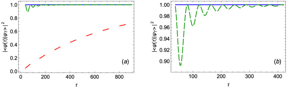
Figure S2: (a) Fidelity as a function of the passage time $\tau$ for three different control strategies, invariant-based (blue-solid line), FAQUAD (green-dashed line), and linear (red-dotted line). (b) Close-up for short times. Parameter values as in Fig. S1.

In Fig. S2(a)-(b) we plot the fidelity $\mathcal{F}=|\langle\psi(\tau)|\psi_{T}\rangle|^{2}$ of the final evolved state with the target final ground state $|\psi_{T}\rangle=|-(\tau)\rangle$ for three different drivings. This includes the invariant-based reverse engineering, fast quasi-adiabatic (FAQUAD) [65], and linear drivings of the control $h_{z}(t)$ as a function of the duration time $\tau$. The corresponding controls are depicted in Fig. S1(b) for the minimum $\tau$. A simple linear ramp leads to a very bad fidelity and only in extremely slow processes is able to reach the desired state $|-(\tau\rangle)$. A more sophisticated protocol, the FAQUAD, delocalizes the transition probability along the whole dynamical process and allows it to reach $|-(\tau\rangle)$ at shorter times, however, when the process is no longer adiabatic this process also fails leading to a lessening of the fidelity. On the contrary, the invariant-based formalism leads to $h_{z}(t)$ protocol that drives the system to the final target state, regardless of the evolved time $\tau$. In order to find solutions with real functions the condition

$$f_{z}^{2}+\frac{\dot{f}_{z}^{2}}{h_{x}^{2}}\leq K\quad\forall t$$ (S24)

must be satisfied, see Eq. (S22). This sets a minimum final time $\tau_{\rm min}$ that depends on the ansatz to interpolate $f_{z}(t)$.

II.1 I. Adiabatic perturbation theory

In the limit of slow parametric changes, we can find an approximate solution of the Scrhödinger equation,

$$i\partial_{t}\ket{\psi}=\hat{H}\ket{\psi},$$ (S25)

where $\ket{\psi}$ is the wavefunction. Since the Hamiltonian is changed slowly, it is convenient to write the wavefunction in the adiabatic (instantaneous) basis,

$$\ket{\psi(t)}=a_{+}(t)\ket{+(t)}+a_{-}(t)\ket{-(t)},$$ (S26)

with the eigenstates $\ket{\pm(t)}$ given by (I). The eigenstates and corresponding eigenenergies implicitly depend on time through the coupling parameter. Substituting expansion (S26) into (S25), and multiplying it by $\bra{+}$ (to shorten the notation we drop the $t$ dependence in the states),

$$i\partial_{t}a_{+}(t)+ia_{-}(t)\bra{+}\partial_{t}\ket{-}=E_{+}(t)a_{+}(t).$$ (S27)

We now perform a gauge transformation,

$$a_{\pm}(t)=\alpha_{\pm}(t)\exp{\left[-i\Theta_{\pm}(t)\right]},$$ (S28)

where

$$\Theta_{\pm}(t)=\int_{t_{i}}^{t}d\tau E_{\pm}(\tau).$$ (S29)

The lower integration limit of the previous expression is arbitrary. Under this transformation, the Schrödinger equation becomes

$$\dot{\alpha}_{+}(t)=-\alpha_{-}(t)\bra{+}\partial_{t}\ket{-}\exp{\left[i(\Theta_{+}(t)-\Theta_{-}(t))\right]},$$ (S30)

which can also be rewritten as an integral equation

$$\alpha_{+}(t)=-\int_{t_{i}}^{t}dt^{\prime}\alpha_{-}(t^{\prime})\bra{+}\partial_{t^{\prime}}\ket{-}\exp{\left[i(\Theta_{+}(t^{\prime})-\Theta_{-}(t^{\prime}))\right]}.$$ (S31)

We now compute the first order correction to the wavefunction assuming for simplicity that initially the system is in the pure state $\ket{-}$, so that $\alpha_{-}(0)=1$ and $\alpha_{+}(0)=0$. In the slowly-varying parameter limit, we assume that the $\ket{+}$ state will be barely populated, and derive

$$\alpha_{+}(t)\approx-\int_{t_{i}}^{t}dt^{\prime}\bra{+}\partial_{t^{\prime}}\ket{-}\exp{\left[i(\Theta_{+}(t^{\prime})-\Theta_{-}(t^{\prime}))\right]}.$$ (S32)

The transition probability to the excited state is determined by $\lvert\alpha_{+}(\tau)\rvert^{2}$. Using the standard rules for evaluating the integrals of fast oscillating functions we find

$$\alpha_{+}(\tau)\approx\left[i\frac{\bra{+}\partial_{t}\ket{-}}{E_{+}(t)-E_{-}(t)}-\frac{1}{E_{+}(t)-E_{-}(t)}\frac{d}{dt}\frac{\bra{+}\partial_{t}\ket{-}}{E_{+}(t)-E_{-}(t)}+...\right]e^{i(\Theta_{+}(t)-\Theta_{-}(t))}\Bigg{\rvert}^{\tau}_{t_{i}}.$$ (S33)

The first term should dominate in slow processes. In particular, for the Landau-Zener Hamiltonian, this term takes the form

$$\alpha_{+}(\tau)\approx i\left[\frac{h_{x}\dot{h}_{z}(\tau)}{\left(h_{x}^{2}+h_{z}(\tau)^{2}\right)^{3/2}}e^{i(\Theta_{+}(\tau)-\Theta_{-}(\tau))}-\frac{h_{x}\dot{h}_{z}(0)}{\left(h_{x}^{2}+h_{z}(0)^{2}\right)^{3/2}}\right].$$ (S34)

Now, from Eq.(S22), we also obtain

$$\dot{h}_{z}(t)=\frac{\left(\dddot{f}_{z}+\dot{f}_{z}h_{x}^{2}\right)\sqrt{c_{1}-f_{z}^{2}-\left(\frac{\dot{f}_{z}}{h_{x}}\right)^{2}}+\left(\ddot{f}_{z}+f_{z}h_{x}^{2}\right)\frac{\dot{f}_{z}f_{z}h_{x}^{2}+\ddot{f}_{z}\dot{f}_{z}}{h_{x}^{2}\sqrt{c_{1}-f_{z}^{2}-\left(\frac{\dot{f}_{z}}{h_{x}}\right)^{2}}}}{c_{1}-f_{z}^{2}-\left(\frac{\dot{f}_{z}}{h_{x}}\right)^{2}}\frac{1}{h_{x}},$$ (S35)

but given the boundary conditions $\dot{f}_{z}(t_{B})=\ddot{f}_{z}(t_{B})=0$,

$$\dot{h}_{z}(t_{B})=\frac{\dddot{f}_{z}(t_{B})\sqrt{h_{x}^{2}+h_{z}(t_{B})^{2}}}{h_{x}^{2}}.$$ (S36)

The auxiliary function $f_{z}$ is constructed as a function of the dimensionless variable $s=t/\tau$. Consequently, the third derivative of $f_{z}$ scales as

$$\dddot{f}_{z}(t)=\left(\frac{ds}{dt}\right)^{3}\frac{d^{3}}{ds^{3}}f(s)=\frac{1}{\tau^{3}}\frac{d^{3}}{ds^{3}}f(s).$$ (S37)

Since $h_{x}$ and $h_{z}(t_{B})$ are unrelated to the protocol duration $\tau$, the first derivative of $h_{z}$ is also proportional to $1/\tau^{3}$ at the boundaries, according to Eq. (S37). Thus, when examining Eq. (S35), it becomes clear that, for sufficiently long times for the adiabatic approximation to hold in every momentum subspace, the probability of excitation in each of the subspace $\lvert\alpha_{+}(\tau)\rvert^{2}$ scales as $\tau^{-6}$. Notably, the boundary conditions for the third derivative of the auxiliary function are entirely arbitrary. Specifically, they can be chosen to be 0. In such a case, the second term in Eq. (S34) becomes dominant, ultimately leading to an excitation coefficient $\alpha_{+}(\tau)$ proportional to the fourth derivative of the auxiliary function, thus leading to a scaling of the excitation probability following $\tau^{-8}$. More generally, if $k$ successive derivatives of $f_{z}$ are engineered to be 0 at the boundaries by choosing a higher order polynomial function with the right coefficients, the probability of excitation should follow a $\tau^{-2k}$ scaling.

II.2 II. Minimum evolution time and the quantum speed limit

Taking polynomial of degree $5$ as an ansatz for $f_{z}(t)$, we obtain (here using $c_{1}=1$)

$$f(t)=\frac{1}{\tau^{5}}\left(-g_{0}\frac{1}{\sqrt{\Delta^{2}+g_{0}^{2}}}(t-\tau)^{3}(6t^{2}+3\tau t+\tau^{2})+g_{1}\frac{1}{\sqrt{\Delta^{2}+g_{1}^{2}}}t^{3}(6t^{2}-15t\tau+10\tau^{2})\right)$$ (S38)

where $h_{z}(t)\equiv g(t)$, so that $g(t=0)=g_{0}$ and $g(\tau)=g_{1}$, and $h_{x}\equiv\Delta$. From this expression, one finds $g(t)$ using Eq. (S22). The expression for the control is a bit involved,

$$g(t)=\frac{N(t)}{M(t)}$$ (S39)

with

$$N(t)= \left(g_{1}\frac{t(6t^{2}(20+\Delta^{2}t^{2})-15t(12+\Delta^{2}t^{2})\tau+10(6+\Delta^{2}t^{2})\tau^{2})}{\sqrt{\Delta^{2}+g_{1}^{2}}}\right.$$ (S40)

$$\left.+g_{0}\frac{(-6t^{3}(20+\Delta^{2}t^{2})+15t^{2}(12+\Delta^{2}t^{2})\tau-10t(6+\Delta^{2}t^{2})\tau^{2}+\Delta^{2}\tau^{5})}{\sqrt{\Delta^{2}+g_{0}^{2}}}\right)$$ (S41)

and

$$M(t) =\Delta\left(\tau^{5}\left[1-\frac{900(g_{0}(\Delta^{2}+g_{0})^{-1/2}-g_{1}(\Delta^{2}+g_{1}^{2})^{-1/2})^{2}t^{4}(t-\tau)^{4}}{\Delta^{2}\tau^{10}}\right.\right.$$ (S42)

$$\left.\left.-\frac{1}{\tau^{10}}\left(g_{1}(\Delta^{2}+g_{1}^{2})^{-1/2}t^{3}(-6t^{2}+15t\tau-10\tau^{2})+g_{0}(\Delta^{2}+g_{0}^{2})^{-1/2}(t-\tau)^{3}(6t^{2}+3t\tau+\tau^{2})\right)^{2}\right]^{1/2}\right)$$ (S43)

Based on the aforementioned ansatz, this method works as long as the term inside the square root of $M(t)$ is non-negative. In order to determine the minimum evolution time, $\tau_{\rm min}$, we consider that $g_{1}=-g_{0}$. Considering these parameters, the term inside the square root in $M(t)$ becomes negative for $\tau<\tau_{\rm min}$, where

$$\tau_{\rm min}=\frac{15g_{0}}{4\Delta\sqrt{\Delta^{2}+g_{0}^{2}}}$$ (S44)

For $\Delta\ll g_{0}$, this leads to $\tau_{\rm min}\approx 15/(4\Delta)\approx 15/(4\pi)\ \pi/\Delta\approx 1.2\tau_{\rm QSL}$ with $\tau_{\rm QSL}=\pi/\Delta$ the quantum speed limit. Note that this specific value depends on the initial ansatz for $f_{z}(t)$. This means that $\tau_{\rm min}$ can be further reduced considering other functional forms for $f_{z}(t)$.

III C. Quantum many-body systems

III.1 I. Application to the transverse-field Ising model

We consider the Transverse Field Ising Model in one dimension with periodic boundary conditions, this is a chain of $N$ spin-$1/2$ particles separated by a distance $a$ with the ends of the chain connected. The Hamiltonian of such a system is given by

$$\hat{H}_{\rm TFIM}=-J\sum_{i=1}^{N}(g\hat{\sigma}_{i}^{x}+\hat{\sigma}_{i}^{z}\hat{\sigma}_{i+1}^{z}),$$ (S45)

where $\hat{\sigma}_{i}^{x,y,z}$ are the usual Pauli matrices for the spin-$1/2$ particle located at the site $i$, $J$ describes the energy scale of the interaction Hamiltonian, and $g$ is a dimensionless parameter related to the interaction of the spin-$1/2$ particles with an external magnetic field. We assume that $g$ is a controllable parameter. Pauli matrices at two different sites commute. The above system can be mapped to a model of spinless fermions using the Jordan-Wigner transformation, in which a spin up (down) at any site is mapped to the presence (absence) of a spinless fermion at that site. This is done by introducing a fermion annihilation operator $\hat{c}_{i}$ such that

$$\hat{\sigma}_{i}^{x} =1-2\hat{c}_{i}^{\dagger}\hat{c}_{i},$$ (S46)

$$\hat{\sigma}_{i}^{z} =-(\hat{c}_{i}+\hat{c}_{n}^{\dagger})\prod_{j<i}(1-2\hat{c}_{j}^{\dagger}\hat{c}_{m}),$$ (S47)

and $\{\hat{c}_{i},\hat{c}_{j}\}=\{\hat{c}_{i}^{\dagger},\hat{c}_{j}^{\dagger}\}=0$ and $\{\hat{c}_{j},\hat{c}_{i}^{\dagger}\}=\delta_{i,j}$. In this manner, the Hamiltonian can be rewritten as

$$H_{\rm TFIM}=-J\sum_{i=1}^{N}\left\{g(1-2\hat{c}_{i}^{\dagger}c_{i})+\left[(\hat{c}_{i}+\hat{c}_{i}^{\dagger})\prod_{j<i}(1-2\hat{c}_{j}^{\dagger}\hat{c}_{j})\right]\left[(\hat{c}_{i+1}+\hat{c}_{i+1}^{\dagger})\prod_{k<i+1}(1-2\hat{c}_{k}^{\dagger}\hat{c}_{k})\right]\right\}.$$ (S48)

Now, using the commutation relations, we find

$$(\hat{c}_{i}+\hat{c}_{i}^{\dagger})\prod_{j<i}(1-2\hat{c}_{j}^{\dagger}\hat{c}_{j})(\hat{c}_{i+1}+\hat{c}_{i+1}^{\dagger})\prod_{k<i+1}(1-2\hat{c}_{k}^{\dagger}\hat{c}_{k}) =(\hat{c}_{i}+\hat{c}_{i}^{\dagger})(\hat{c}_{i+1}+\hat{c}_{i+1}^{\dagger})(1-2\hat{c}_{i}^{\dagger}c_{i})$$ (S49)

$$=-(\hat{c}_{i+1}+\hat{c}_{i+1}^{\dagger})(\hat{c}_{i}+\hat{c}_{i}^{\dagger})(1-2\hat{c}_{i}^{\dagger}\hat{c}_{i})$$ (S50)

$$=-(\hat{c}_{i+1}+\hat{c}_{i+1}^{\dagger})(\hat{c}_{i}^{\dagger}-\hat{c}_{i})=\hat{c}_{i+1}\hat{c}_{n}+\hat{c}_{n}^{\dagger}c_{i+1}+{\rm H.c.},$$ (S51)

so that the Hamiltonian reads

$$\hat{H}_{\rm TFIM}=-J\sum_{i=1}^{N}\left(g/2-g\hat{c}_{i}^{\dagger}\hat{c}_{i}+\hat{c}_{i+1}\hat{c}_{i}+\hat{c}_{i}^{\dagger}\hat{c}_{i+1}+{\rm H.c.}\right).$$ (S52)

Note that, by taking $N$ even, the $\hat{c}_{i}$’s satisfy either periodic boundary conditions $\hat{c}_{N+1}=\hat{c}_{1}$ (negative parity), or antiperiodic boundary conditions (positive parity), $\hat{c}_{N+1}=-\hat{c}_{1}$. We select the positive parity (as it contains the ground state for $N$ even in the paramagnetic phase). We continue the diagonalization by Fourier transforming these fermionic operators (from now on subscript $k$ or $q$ refers to Fourier transformed, in contrast to $i$ or $j$ for the original operators):

$$\hat{c}_{j}=\frac{e^{-i\pi/4}}{\sqrt{N}}\sum_{k}\hat{c}_{k}e^{ikja},$$ (S53)

where the sum runs from negative to positive $k$ values ($a$ accounts for the spin inter-spacing). The values that $k$ can take are

$$k_{j}=\pm\frac{(2j-1)\pi}{Na}\ \ j=1,2,\ldots,N/2.$$ (S54)

This transformations satisfies $\hat{c}_{N+1}=-\hat{c}_{1}$. In particular, we find the following relations

$$\hat{c}_{j}^{\dagger}\hat{c}_{j} =\frac{1}{N}\sum_{k,q}\hat{c}_{k}^{\dagger}\hat{c}_{q}e^{-ija(k-q)}$$ (S55)

$$\hat{c}_{j+1}\hat{c}_{j} =\frac{e^{-i\pi/2}}{N}\sum_{k,q}\hat{c}_{k}\hat{c}_{q}e^{ija(k+q)}e^{ika}$$ (S56)

$$\hat{c}^{\dagger}_{j}\hat{c}_{j+1} =\frac{1}{N}\sum_{k,q}\hat{c}_{k}^{\dagger}\hat{c}_{q}e^{-ija(k-q)}e^{-ika}$$ (S57)

$$\hat{c}_{j}^{\dagger}\hat{c}_{j+1}^{\dagger} =\frac{e^{i\pi/2}}{N}\sum_{k,q}\hat{c}_{k}^{\dagger}\hat{c}_{q}^{\dagger}e^{-ija(k+q)}e^{-ika}$$ (S58)

$$\hat{c}^{\dagger}_{j+1}\hat{c}_{j} =\frac{1}{N}\sum_{k,q}\hat{c}_{k}^{\dagger}\hat{c}_{q}e^{-ija(k-q)}e^{-ika}$$ (S59)

which upon the sum over all the sites leads to

$$\sum_{j=1}^{N}\hat{c}_{j}^{\dagger}\hat{c}_{j} =\frac{1}{N}\sum_{j=1}^{N}\sum_{k,q}\hat{c}_{j}^{\dagger}\hat{c}_{q}e^{-ija(k-q)}=\sum_{k}\hat{c}_{k}^{\dagger}\hat{c}_{k},$$ (S60)

where we have used $\sum_{j=1}^{N}e^{-ija(k-q)}=\delta_{k,q}N$ and the sum over $k$ has been taken for positive and negative values. Similarly,

$$\sum_{j=1}^{N}\hat{c}_{j+1}c_{j} =e^{-i\pi/2}\sum_{k}\hat{c}_{k}\hat{c}_{-k}e^{ika}$$ (S61)

$$\sum_{j=1}^{N}\hat{c}^{\dagger}_{j}\hat{c}_{j+1} =e^{i\pi/2}\sum_{k}\hat{c}_{k}^{\dagger}\hat{c}_{-k}^{\dagger}e^{-ika}$$ (S62)

$$\sum_{j=1}^{N}\hat{c}_{j}^{\dagger}\hat{c}_{j+1} =\sum_{k}\hat{c}_{k}^{\dagger}\hat{c}_{k}e^{-ika}$$ (S63)

$$\sum_{j=1}^{N}c_{j+1}^{\dagger}c_{j} =\sum_{k}\hat{c}_{k}^{\dagger}\hat{c}_{k}e^{ika}.$$ (S64)

Introducing the previous expressions into Eq. (S52), we obtain

$$\hat{H}_{\rm TFIM} =J\sum_{k}\left[-g+2g\hat{c}_{k}^{\dagger}\hat{c}_{k}-e^{-i\pi/2}\hat{c}_{k}\hat{c}_{-k}e^{ika}-\hat{c}_{k}^{\dagger}\hat{c}_{k}e^{ika}-e^{i\pi/2}\hat{c}_{-k}^{\dagger}\hat{c}_{k}^{\dagger}e^{-ika}-\hat{c}_{k}^{\dagger}\hat{c}_{k}e^{-ika}\right]$$ (S65)

$$=J\sum_{k}\left[-g+(2g-e^{ika}-e^{-ika})\hat{c}_{k}^{\dagger}\hat{c}_{k}-e^{-i\pi/2}\hat{c}_{k}\hat{c}_{-k}e^{ika}-e^{i\pi/2}\hat{c}^{\dagger}_{-k}\hat{c}_{k}^{\dagger}e^{-ika}\right].$$ (S66)

Now using

$$\sum_{k}\left(i\hat{c}_{k}\hat{c}_{-k}e^{ika}-i\hat{c}_{-k}^{\dagger}\hat{c}_{k}^{\dagger}e^{-ika}\right) =\sum_{k>0}\left(ie^{ika}\hat{c}_{k}\hat{c}_{-k}-ie^{-ika}\hat{c}^{\dagger}_{-k}\hat{c}_{k}^{\dagger}+ie^{-ika}\hat{c}_{-k}\hat{c}_{k}-ie^{ika}\hat{c}_{k}^{\dagger}\hat{c}_{-k}^{\dagger}\right)$$ (S67)

$$=\sum_{k>0}(-2)\sin ka\left(\hat{c}_{k}\hat{c}_{-k}+\hat{c}_{-k}^{\dagger}\hat{c}_{k}^{\dagger}\right)=-\sum_{k}\sin ka\left(\hat{c}_{k}\hat{c}_{-k}+\hat{c}_{-k}^{\dagger}\hat{c}_{k}^{\dagger}\right),$$ (S68)

we finally obtain

$$\hat{H}_{\rm TFIM} =J\sum_{k}\left[-g+2(g-\cos ka)\hat{c}_{k}^{\dagger}\hat{c}_{k}-\sin ka\left(\hat{c}_{k}\hat{c}_{-k}+\hat{c}_{-k}^{\dagger}\hat{c}_{k}^{\dagger}\right)\right].$$ (S69)

Let us now define a fermionic mode $\Psi^{\dagger}_{k}=(\hat{c}_{k}^{\dagger},\hat{c}_{-k})$, so that we can write

$$\hat{H}_{\rm TFIM}=\sum_{k>0}\Psi^{\dagger}_{k}\hat{H}_{k}\Psi_{k}$$ (S70)

where $\hat{H}_{k}$ is given by

$$\hat{H}_{k}=h_{k}^{z}(g)\frac{\hat{\sigma}^{k}_{z}}{2}+h_{k}^{x}\frac{\hat{\sigma}^{k}_{x}}{2},$$ (S71)

with $\hat{\sigma}^{k}_{z}=\ket{1}_{k}\bra{1}_{k}-\ket{0}_{k}\bra{0}_{k}$, $h_{k}^{z}(g)=4J(g-\cos(ka))$, and $h_{k}^{x}=4J\sin(ka)$.

The control of $g(t)$ is designed to follow the eigenstates of the invariant associated with the lowest energy Hamiltonian, i.e.,

$$\hat{H}_{k_{0}}=2J\left[g-\cos\left(\frac{\pi}{N}\right)\right]\hat{\sigma}_{z}^{k_{0}}+2J\sin\left(\frac{\pi}{N}\right)\hat{\sigma}_{x}^{k_{0}}.$$ (S72)

According to Eq. (S22), $g(t)$ is defined as

$$g(t)=\cos\left(\frac{\pi}{N}\right)+\frac{1}{4J}\frac{\ddot{f}_{z}+f_{z}\left(4J\sin\left(\frac{\pi}{N}\right)\right)^{2}}{\sqrt{K-f_{z}^{2}-\frac{\dot{f}_{z}^{2}}{\left(4J\sin\left(\frac{\pi}{N}\right)\right)^{2}}}}\frac{1}{\left(4J\sin\left(\frac{\pi}{N}\right)\right)},$$ (S73)

with $f_{z}=f_{z}(t)$ any arbitrary function that fulfills the boundary conditions given by Eq. (S23)

III.2 II. Application to the long-range Kitaev chain

Let us now consider the case of the long-range Kitaev chain of fermionic particles with periodic boundary conditions. The Hamiltonian reads

$$\hat{H}_{\rm LRK}=-J\sum_{i=1}^{N}\left[\sum_{r>0}\left(J_{r}\left(\hat{c}_{i}^{\dagger}\hat{c}_{i+r}+\hat{c}_{i+r}^{\dagger}\hat{c}_{i}\right)+d_{r}\left(\hat{c}_{i}\hat{c}_{i+r}+\hat{c}_{i+r}\hat{c}_{i}\right)\right)-g(t)\hat{n}_{i}\right],$$ (S74)

where $\hat{c}_{i}$ is the fermionic annihilation operator at site $i$, $\hat{n}_{i}=\hat{c}_{i}^{\dagger}\hat{c}_{i}$, $g(t)$ is a dimensionless controllable parameter related to the chemical potential, and

$$J_{r}=\frac{1}{N\bar{r}^{\alpha}},\hskip 17.07164ptd_{r}=\frac{1}{N\bar{r}^{\beta}},$$ (S75)

where, given the periodic boundary conditions, $\bar{r}=a{\rm min}(r,N/2-r)$. The Hamiltonian is quadratic in fermions and can hence be exactly solved by a Fourier Transformation in the momentum space $\hat{c}_{i}=\frac{1}{\sqrt{N}}\sum_{n=0}^{N-1}e^{-ik_{n}x_{i}}\hat{c}_{k_{n}}$. Assuming anti-periodic boundary conditions $(\hat{c}_{i}=-\hat{c}_{i+N})$, the momenta modes are quantized as $k_{n}=(2\pi/Na)(n-1/2)$. In this basis, the Hamiltonian can be written as

$$\hat{H}_{\rm LRK}=\sum_{k>0}\Psi^{\dagger}_{k}\hat{H}_{k}\Psi_{k},$$ (S76)

where the sub-index in $k_{n}$ has been droped for simplicity, $\Psi^{\dagger}=(\hat{c}_{k}^{\dagger},\hat{c}_{-k})$ and $\hat{H}_{k}=h_{z,k}\hat{\sigma}_{z}^{k}/2+h_{x,k}\hat{\sigma}_{x}^{k}/2$. Each subspace of momentum $k$ evolves independently, with $h_{z,k}=g-4J\sum_{r>0}J_{r}\cos\left(kra\right)$ and $h_{x,k}=-2J\sum_{r>0}d_{r}\sin(kra)$.

Just as in the application to the TFIM, the invariant protocol is designed to drive the system with the smallest energy gap ($k_{0}$) with unit fidelity.

III.3 III. Details on the scaling analysis

In the main text, we have demonstrated the scaling behavior of the density of excitations, denoted as $n$, which is defined as $n=1-\frac{2}{N}\sum_{k>0}|\langle\phi_{k,0}|\psi_{k}(\tau)\rangle|^{2}$. This scaling has been examined with respect to two key parameters: the rescaled quench time, $\tau/\tau_{QSL}$, and the total number of interacting particles, denoted as $N$. For the sake of completeness and a comprehensive understanding of the system’s behavior, we also present an analysis of the scaling properties of the infidelity, denoted as $\mathcal{I}$, which is defined as $\mathcal{I}=1-\mathcal{F}$. Here, $\mathcal{F}$ represents the fidelity and is defined as $\mathcal{F}=\langle\phi_{0}(g_{1})|\psi(\tau)\rangle|^{2}$. We perform this analysis across the same set of parameters, namely $\tau/\tau_{QSL}$ and $N$, in Fig.S3. This examination serves to verify the equivalence between the scaling behaviors of these two fundamental measures, providing a more comprehensive perspective on the quantum phase transitions under investigation.

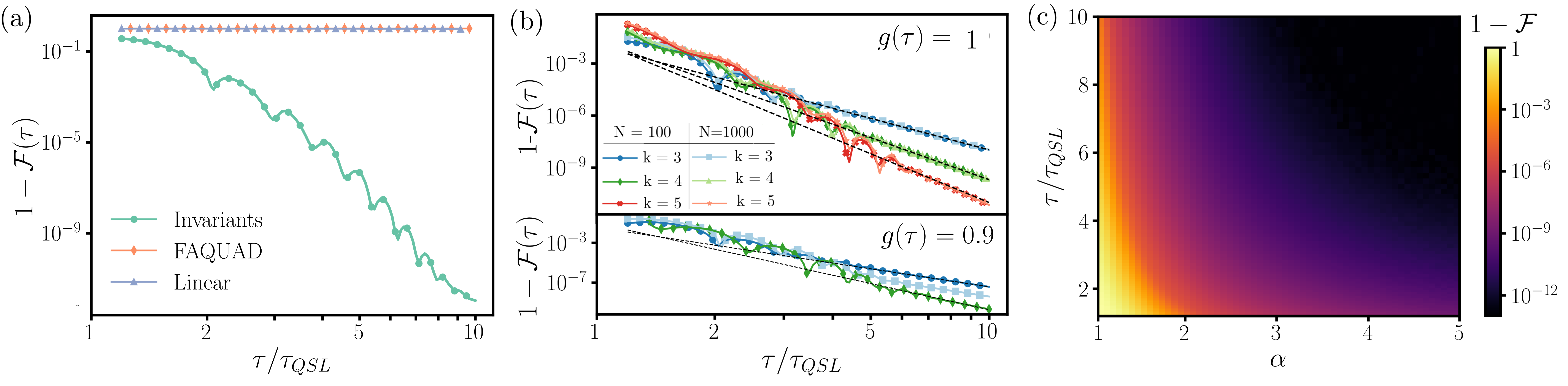
Figure S3: (a) Infidelity for fixed $N=200$ spins as a function of the rescaled quench time $\tau/\tau_{QSL}$ (log-log scale) for the TFIM and the three protocols. Parameter values: $\lambda=1$, $J=1$, $g(0)=10$, $g(\tau)=0$. (b) Scaling of the infidelity for the TFIM invariant protocol for $N=100$ and $N=1000$ as a function of the rescaled quench time for protocols with $k=3$, $k=4$ and $k=5$. The final value of the control parameter is $g(\tau)=1$ (top) and $g(\tau)=0.9$ (bottom). The polynomial behavior cannot be observed for $g(\tau)=0.9$ in the cases $k=4$ $N=1000$ or $k=5$ due to limitations in numerical precision. (c) Scaling of the infidelity in the LRK for $N=100$ spins as a function of the rescaled quench time and the long-range exponent $\alpha$. Parameter values: $\beta\rightarrow\infty$, $J=2$, $g(0)=10$, $g(\tau)=0$.

III.4 IV. Details on robustness

The robustness of the invariant-based control is studied in the TFIM. The Hamiltonian of interest can be written as

$$\hat{H}_{\rm TFIM}=-J\left(g(t)\sum_{i=1}^{N}\hat{\sigma}_{i}^{x}+\sum_{i}^{N}\lambda_{i}\hat{\sigma}_{i}^{z}\hat{\sigma}_{i+1}^{z}\right).$$ (S77)

Note that we have now included site-dependent interaction strength $\lambda_{i}$. In addition, as mentioned in the main text, we analyze the impact on noisy controls, namely, $g(t)\rightarrow g(t)+\eta(t)$ so that $\eta(t)$ represents a standard white Gaussian noise, $\langle\eta(t)\rangle=0$ and $\langle\eta(t)\eta(t^{\prime})\rangle=W^{2}$ being $W$ its strength. The impact of these two different imperfections is studied individually.

Noisy control.—

First, the noisy control can be tackled following similar steps as in Ref. [31]. For this, we take $\lambda_{i}=1\ \forall i$, i.e. no interaction disorder. The wavefunction evolves according to

$$\frac{d}{dt}\ket{\psi(t)}=-i(\hat{H}_{0}(t)+\eta(t)\hat{H}_{1})\ket{\psi(t)}$$ (S78)

where $\hat{H}_{0}(t)$ is the sure and ideal TFIM Hamiltonian, while $\hat{H}_{1}=-J\sum_{i=1}^{N}\hat{\sigma}_{i}^{x}$. Averaging over the noise, the state is described in terms of a density matrix $\hat{\rho}(t)$ which obeys the master equation

$$\frac{d}{dt}\hat{\rho}(t)=-i[\hat{H}_{0}(t),\hat{\rho}(t)]-\frac{W^{2}}{2}\left[\hat{H}_{1},[\hat{H}_{1},\hat{\rho}(t)]\right].$$ (S79)

Upon Jordan-Wigner and Fourier transformations, we arrive at the master equation for the density matrix for the $k$ subspace

$$\frac{d}{dt}\hat{\rho}_{k}(t)=-i[\hat{H}_{k}(t),\hat{\rho}_{k}(t)]-\frac{W^{2}}{2}[\hat{H}_{1,k},[\hat{H}_{1,k},\hat{\rho}_{k}(t)]]$$ (S80)

with $\hat{H}_{1,k}=2J\hat{\sigma}_{z}^{k}$, while $\hat{H}_{k}(t)$ has the same form as above. The results for different values of $W$ are plotted in the main text (cf. Fig. 2).

Random disorder.—

Second, we examine the impact of interaction-strength disorder. For that, the dimensionless coupling strength $\lambda_{i}$ is considered to be a uniform random variable such that $\langle\lambda_{i}\rangle=1$ and $\lambda_{i}\in[1-\Lambda,1+\Lambda]$, and independent among sites. Note that one could consider a global noisy coupling strength $\lambda\rightarrow\lambda+\eta(t)$ for all sites, whose impact would be similar to a noisy control. This interaction-strength disorder is tackled by relying on a Jordan-Wigner transformation of the TFIM. The fermionic Hamiltonian results in

$$\hat{H}_{\rm TFIM}=-J\left[\sum_{i=1}^{N-1}\lambda_{i}(c_{i}^{\dagger}c_{i+1}^{\dagger}+c_{i}^{\dagger}c_{i+1}+{\rm H.c})-2g\sum_{i=1}^{N}c_{i}^{\dagger}c_{i}\right]+J\lambda_{N}(c_{N}^{\dagger}c_{1}^{\dagger}+c_{N}^{\dagger}c_{1}+{\rm H.c.}),$$ (S81)

since we consider periodic boundary conditions. Since the couplings are not homogeneous, this model cannot be brought into a collection of independent Landau-Zener or two-level systems in the momentum space. Instead, one needs to solve this fermionic system, which can be written as

$$\hat{H}_{\rm TFIM}=\Psi^{\dagger}\hat{H}_{f}\Psi$$ (S82)

with $\Psi^{\dagger}=(\hat{c}_{1}^{\dagger},\hat{c}_{2}^{\dagger},\ldots,\hat{c}_{N}^{\dagger},\hat{c}_{1},\hat{c}_{2},\ldots,\hat{c}_{N})$ which fulfill the fermionic anti-commutation relations $\{\Psi_{i},\Psi_{j}^{\dagger}\}=\delta_{i,j}$, and

$$\hat{H}_{f}=\begin{bmatrix}A&B\\ -B&-A\end{bmatrix}$$ (S83)

with $A$ and $B$ symmetric and anti-symmetric real matrices with matrix-elements $A_{i,i}=Jg$, $A_{i,i+1}=A_{i+1,i}=-J\lambda_{i}/2$, but $A_{N,1}=A_{1,N}=J\lambda_{N}/2$, while $B_{i,i+1}=-B_{i+1,i}=-J\lambda_{i}/2$, and $B_{1,N}=-B_{N,1}=J\lambda_{N}/2$. In the Heisenberg picture, and employing a Bogoliubov operator $c_{i,H}(t)=\sum_{\mu=1}^{N}(u_{i,\mu}(t)\gamma_{\mu}+v_{i,\mu}^{*}(t)\gamma_{\mu}^{\dagger})$ with fermionic operators $\gamma_{\mu}$, it can be shown that the coherent dynamics is fully characterized by the evolution of the coefficients

$$\dot{u}_{i,\mu} =-2i\sum_{j=1}^{N}\left[A_{i,j}(t)u_{j,\mu}(t)+B_{i,j}v_{j,\mu}(t)\right]$$ (S84)

$$\dot{v}_{i,\mu} =2i\sum_{j=1}^{N}\left[A_{i,j}(t)v_{j,\mu}(t)+B_{i,j}u_{j,\mu}(t)\right]$$ (S85)

with the initial condition set at by the eigenvalue problem in Eq. (S83) at $g(t=0)=g_{0}$. Note that the time-dependent control enters via the symmetric matrix $A(t)$, and $u(t)$ and $v(t)$ are $N\times N$ matrices that satisfy $u^{\dagger}(t)u(t)+v^{\dagger}(t)v(t)=\mathbb{I}$ at all times to ensure the fermionic anti-commutation relation.

We then numerically solve the coupled differential equations under the protocol $g(t)$ for $u_{i\mu}(t)$ and $v_{i\mu}(t)$ for different disorder realizations and then average the results. We compute the density of excitations, which in the original spin representation reads as

$$n_{d}=\frac{1}{N}\sum_{i=1}^{N}\bra{\psi(\tau)}\frac{1}{2}(1-\hat{\sigma}^{z}_{i}\hat{\sigma}^{z}_{i+1})\ket{\psi(\tau)}.$$ (S86)

In the fermionic Jordan-Wigner representation, it results in $n_{d}=\frac{1}{2N}\sum_{i=1}^{N-1}(1-[(v(\tau)-u(\tau))(u^{\dagger}(\tau)+v^{\dagger}(\tau))]_{i+1,i})+\frac{1}{2N}(1-[(v(\tau)-u(\tau))(u^{\dagger}(\tau)+v^{\dagger}(\tau))]_{1,N})$.

Recall that the invariant-based protocol is not altered, i.e. we perform the protocol designed for an ideal TFIM (without the disorder, $\Lambda=0$). The average density of excitations is plotted in the main text (cf. Fig. 2).