Neural Koopman prior for data assimilation

Abstract

With the increasing availability of large scale datasets, computational power and tools like automatic differentiation and expressive neural network architectures, sequential data are now often treated in a data-driven way, with a dynamical model trained from the observation data. While neural networks are often seen as uninterpretable black-box architectures, they can still benefit from physical priors on the data and from mathematical knowledge. In this paper, we use a neural network architecture which leverages the long-known Koopman operator theory to embed dynamical systems in latent spaces where their dynamics can be described linearly, enabling a number of appealing features. We introduce methods that enable to train such a model for long-term continuous reconstruction, even in difficult contexts where the data comes in irregularly-sampled time series. The potential for self-supervised learning is also demonstrated, as we show the promising use of trained dynamical models as priors for variational data assimilation techniques, with applications to e.g. time series interpolation and forecasting.

I Introduction

The evergrowing amount of historical data for scientific applications has recently enabled to model the evolution of dynamical systems in a purely data-driven way using powerful regressors such as neural networks. While many of the most spectacular results obtained by neural networks rely on the paradigm of supervised learning, this paradigm is limited in practice by the available amount of labelled data, which can be prohibitively costly and difficult to obtain. For example, a number of Earth observation programs that have been launched in the last decade provide huge amounts of sequential (though generally incomplete) satellite multi/hyperspectral images covering the entire Earth’s surface. However, few accurate and reliable labels exist for land cover classification of the ground pixels, although some efforts have been made, e.g. for crop type classification and segmentation [1, 2].

In this context, one can leverage another machine learning paradigm called self-supervised learning (SSL) [3]. It consists in training a machine learning model to solve a pretext task that requires no labels in order to learn informative representations of the data which can be used to solve downstream tasks. When dealing with image data, possible pretext tasks include predicting the relative positions of two randomly selected patches of a same image [4] and predicting which rotation angle has been applied to an image [5]. Many SSL approaches can be labelled as contrastive SSL [6], which means that they aim at learning similar representations for images that are related by transformations such as rotations, crops and color transfers. We refer the interested reader to [7] for a review of self-supervised learning for remote sensing applications.

In our case, since we are dealing with sequential data, we use a natural pretext task which consists in being able to forecast the future state of the data from a given initial condition. This is similar in spirit to recent approaches in natural language processing where a model is trained on completing texts and then used to perform various tasks in zero/few shot, e.g. [8]. Our trained model is used for downstream tasks which can be formulated as inverse problems such as denoising and interpolation. We solve these tasks by minimising a variational cost which uses a trained model as a dynamical prior, contrarily to classical data assimilation techniques [9, 10, 11] which leverage hand-crafted dynamical priors that require domain knowledge, and are not always available. Besides, these priors should be differentiable since any first order optimization algorithm tackling such a problem must be able to differentiate through repeated compositions of the model, which requires careful implementation [12] and is out of reach for many operational systems relying on complex dynamical models [13]. In contrast, neural emulators of the dynamics are de facto implemented in packages supporting automatic differentiation, e.g. Pytorch [14], Tensorflow, JAX, etc. providing effortless access to model derivatives.

For all these reasons, in this paper, we first aim at modelling dynamical systems from observation data using differentiable models. We assume that the state of a dynamical system can be described by a $d$-dimensional state variable $\mathbf{x}\in\mathcal{D}$ with $\mathcal{D}\subset\mathbb{R}^{d}$. Then, assuming the system is governed by an autonomous ordinary differential equation (ODE), one can describe its (discrete) dynamics by a function $F:\mathcal{D}\to\mathcal{D}$ such that $\mathbf{x}_{t+1}=F(\mathbf{x}_{t})$. Although $F$ might be any non-linear function, Koopman operator theory [15] tells us that the model can be described by a linear operator acting in the space of observation functions. Namely, given an observation function $f:\mathcal{D}\to\mathbb{R}$, the so-called Koopman operator $\mathcal{K}$ maps an observation function $f$ to its composition with the dynamics:

$$\mathcal{K}f(\mathbf{x}_{t})\triangleq(f\circ F)(\mathbf{x}_{t})=f(\mathbf{x}_{t+1}).$$ (1)

From this definition, $\mathcal{K}$ is linear because of the linearity of the function space, i.e. for any $f,g:\mathcal{D}\to\mathbb{R}$:

$$\mathcal{K}(f+g)(\mathbf{x}_{t})=(f+g)(\mathbf{x}_{t+1})=\mathcal{K}f(\mathbf{x}_{t})+\mathcal{K}g(\mathbf{x}_{t}).$$ (2)

Yet, the function space being infinite dimensional, the advantage of the linearity of $\mathcal{K}$ comes at the cost of an infinite dimension, which makes it difficult to model in practice. Thus, the key to finding a finite-dimensional representation of the Koopman operator is to look for Koopman invariant subspaces (KIS) [16], i.e. subsets of the function space that are stable by the Koopman operator. There exists a variety of such spaces, but one needs to retrieve nontrivial KIS that give information about the dynamics of the state variable.

Once a KIS is found, the restriction of the Koopman operator to it is a matrix $\mathbf{K}$ which can be interpreted with classical linear algebra tools. Notably, each of the complex eigenvalues of $\mathbf{K}$ is associated to an observation function that is located in the subspace. Let us denote by $\mathbf{K}=\mathbf{V}\mathbf{\Lambda}\mathbf{V}^{-1}$ the complex eigendecomposition of $\mathbf{K}$, with $\mathbf{V}$ the complex eigenvectors and $\mathbf{\Lambda}$ a complex diagonal matrix containing the associated eigenvalues. Predicting $\tau$ steps in the future through the Koopman operator means multiplying the initial latent state vector (obtained with the functions from the invariant subspace) by $\mathbf{K}^{\tau}=\mathbf{V}\mathbf{\Lambda}^{\tau}\mathbf{V}^{-1}$. Therefore, one can see that the eigenvectors associated with an eigenvalue of modulus higher than one will have an exponentially growing contribution, while those with an eigenvalue of modulus smaller than one will exponentially vanish. Only eigenvalues of modulus very close to one will approximately preserve the norm of the latent state in the long run, which might be crucial for time series with clear seasonality or periodicity.

Our approach fits into the Koopman operator framework to model dynamical systems from data. More specifically, our contributions are the following:

1) We perform a synthetic review of the different approaches that have recently been used to compute data-driven approximations of the Koopman operator, emphasizing on the limitations of each of the successive categories of approaches.

2) We refine and extend our own approach to learn a neural Koopman operator, first sketched in [17], with a discussion on the interest of having a (close to) orthogonal Koopman operator and on handling irregular time series.

3) We present several ways to use our model as a fully-differentiable dynamical prior in data assimilation in order to solve inverse problems using automatic differentiation.

4) We present associated results on simulated as well as real-world data. We notably perform a frequency upsampling experiment on fluid flow data. We also show interpolation experiments on satellite image time series using variational data assimilation with our model as a dynamical prior, including in hard scenarios such as irregularly sampled data and transfer to new areas unseen during training.

II Background an related works

II-A Koopman operator theory

In short, the Koopman operator theory [15] states that any dynamical system can be described linearly at the cost of an infinite dimension. However, some methods seek to find a finite-dimensional representation of the Koopman operator. Notably, Dynamic Mode Decomposition [18] (DMD) consists in finding a matrix $\mathbf{A}$ such that the residual $\mathbf{r}_{t}$ in

$$\mathbf{x}_{t+1}=\mathbf{A}\mathbf{x}_{t}+\mathbf{r}_{t}$$ (3)

is as small as possible in the least squares sense. This approach has been theoretically linked to the Koopman mode decomposition in [19], and has known many different variants, e.g. [20, 21, 22]. However, it relies on the implicit assumption that the set of observation functions constituting the identity of the state space is a Koopman invariant subspace (KIS). This assumption can be useful in regions of the state space where the dynamics are close to linear, but it is very unlikely to be generally true. In order to mitigate this shortcoming, the Extended Dynamic Mode Decomposition [23] (EDMD) uses a manually designed dictionary of observable functions from the dynamical system. Common choices of dictionaries include polynomials of the observed variables up to a given degree and sets of radial basis functions. These dictionaries all include the identity of the state space, which trivially allows to make predictions in the state space by projection. Choosing to include only these functions in the dictionary of functions amounts to performing a classical DMD.

Being a generalization of DMD, EDMD can give satisfactory results when the chosen dictionary of functions is well suited to the considered dynamical system. However, a hand-designed dictionary of observables might still not be the most optimal choice, and it is typically very high dimensional. For these reasons, subsequent works have proposed to automatically learn a low-dimensional dictionary of observation functions through machine learning. For example, there is a rich literature on leveraging Reproducing Kernel Hilbert Spaces to obtain approximations of the Koopman operator with some interpretability and theoretical guarantees, e.g. [24, 25, 26].

Other methods [27, 28] jointly learn the parameters of a neural network which computes a set of observation functions and a matrix $\mathbf{K}$ which is the restriction of the Koopman operator to this set. To be able to retrieve the evolution of the state variable from the KIS, they constrain the inclusion of the state space in the subspace along with the learnt functions. This is a convenient trick, yet it restricts those methods since it means assuming that there exists a low-dimensional KIS containing the state functions.

In order to not rely on this assumption anymore, some other works [29, 30, 31, 32, 33, 17] do not constrain a trivial link between the KIS and the state space, and instead train another neural network to reconstruct the state variables from the learnt observation functions. In this case, the network learning the KIS and the network that reconstructs the state space from it form an autoencoder. This framework is theoretically more powerful since it only assumes a nonlinear relationship between the KIS and the state space.

Among these methods, [29], which we refer to as DeepKoopman in this paper, learns an auxiliary network that outputs eigenvalues as a function of the encoded state of the system while others learn a fixed matrix $\mathbf{K}$. [33] learns two distinct matrices for the forward and backward evolutions, in order to favor the consistency of the latent dynamics. A good indicator for the stability of long run predictions is that the eigenvalues of the learnt Koopman matrix should be located on the unit circle, which may encourage us to look for matrices with such eigenvalues. Among those are orthogonal matrices, which have many desirable properties. Most importantly, they lead to constrain the dynamics to be periodic. We detail the reason why this is true in Appendix A.

II-B Orthogonality regularisation

The promotion of orthogonality for the weight matrices of linear layers in neural networks has been long studied. This idea is related to the well-known vanishing gradient and exploding gradient issues. Those get more important as the computational graph gets deeper, e.g. for recurrent neural networks and for very deep residual neural networks [34].

[35] showed that the initialisation of weights as a random orthogonal matrix can be much more effective than the classical random Gaussian initialisation. It was also advocated that the orthogonality of the weight matrices should be promoted during the training phase too. [36] introduced a soft regularisation term for weight matrices $\mathbf{W}$:

$$||\mathbf{W}\mathbf{W}^{T}-\mathbf{I}||^{2}.$$ (4)

This term, which is to be used in a similar way to weight decay [37], was shown to significantly improve the final performance of neural networks in computer vision tasks. [38] compared this term with similar orthogonality-promoting expressions, and showed that they all all brought substantial gains in the performance of deep residual networks.

In our case, constraining the Koopman operator to be orthogonal leads to periodic dynamics, which are of course stable in the long run and useful to model seasonality in time series. Yet, working with an exactly orthogonal $\mathbf{K}$ may not always be desirable, for instance when the data are noisy, or the time series is not exactly periodic (e.g. when there are interannual variations or slower trends in seasonal dynamics), or even not periodic. For these reasons, we will resort to a soft penalization as in (4) instead of enforcing exactly the orthogonality of $\mathbf{K}$.

II-C Variational data assimilation

Variational data assimilation can be used to solve inverse problems involving time series for which one has at disposal a set of possibly noisy and incomplete trajectories $\tilde{\mathbf{x}}$ as well as a dynamical prior and/or a regularisation $\mathcal{R}$ on the distribution of the solution. It consists in finding the complete trajectory that minimizes a variational cost $\mathcal{C}$ of the form

$$\mathcal{C}(\mathbf{x})=\mathcal{D}(\mathbf{x},\tilde{\mathbf{x}})+\mathcal{R}(\mathbf{x})$$ (5)

where $\mathcal{D}$ is a chosen distance, such as a norm of the difference between two elements (restricted to dimensions on which $\tilde{\mathbf{x}}$ is defined). In practice, when all terms are smooth, the cost can be minimised by gradient descent or related first order algorithms. The gradient can be obtained either analytically when tractable, or using automatic differentiation, as made easily accessible by modern computing frameworks, e.g. Pytorch.

Alternatively, one can restrain the search on a set of trajectories defined by a model $\mathcal{M}:\mathbf{x}_{0}\to\mathbf{x}$. In this case, one formulates a cost on the input of the model:

$$\mathcal{C}(\mathbf{x}_{0})=\mathcal{D}(\mathcal{M}(\mathbf{x}_{0}),\tilde{\mathbf{x}})+\mathcal{R}(\mathcal{M}(\mathbf{x}_{0})).$$ (6)

A conceptual view of constrained variational data assimilation is displayed on Figure 1. We refer the interested reader to [9] for an extensive review on data assimilation.

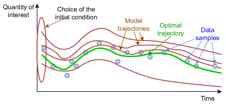
Figure 1: Visual representation of constrained variational data assimilation. It consists in choosing the initial condition from which the model’s trajectory minimises the distance to the sampled data. One could also include a prior in the variational cost on the initial condition, such as the trajectory smoothness.

While variational data assimilation is traditionally used with priors $\mathcal{R}$ that were constructed from physical knowledge of the studied dynamical system, recent works [13, 39] have attempted to leverage machine learning tools to learn a prior in a completely data-driven way. In the second case, the prior is jointly learned with a gradient-based optimization algorithm, further improving performance. Other works [40] have proposed to learn a data-driven surrogate model to predict the residual error of an existing physics-based model, which finally results in a hybrid model. Those models have the advantage of being fully differentiable and implemented in an automatic differentiation framework (e.g. Pytorch or Tensorflow), which means that their associated cost can be differentiated automatically via the chain rule. Overall, linking data assimilation and machine learning is a very hot topic, which has been recently reviewed in [41].

III Proposed methods

III-A Neural network design and training

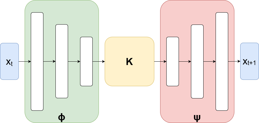
Figure 2: Schematic view of our architecture.

Our architecture for a neural Koopman operator relies on three components : an encoding neural network $\phi$ with a decoder $\psi$ and a matrix $\mathbf{K}\in\mathbb{R}^{d\times d}$. It is graphically represented in Figure 2. The idea is that $(\phi,\psi)$ learns the relationship between the state space and a learnt $d$-dimensional (approximately) Koopman invariant subspace, while $\mathbf{K}$ corresponds to the restriction of the Koopman operator to this space. Our goal is to be able to make long-term predictions of the state by successive multiplications of the encoded initial state, followed by a decoding to come back to the original data space. This translates in equations as

$$\psi(\mathbf{K}^{\tau}\phi(\mathbf{x}_{t}))=\mathbf{x}_{t+\tau}$$ (7)

for any initial condition $\mathbf{x}_{t}$ and time increment $\tau$. We emphasize that $\tau$ does not necessarily have to be an integer since one can easily compute noninteger powers of $\mathbf{K}$ by using its matrix logarithm, as explained in section III-B. The time increment $\tau$ could also very well be negative, enabling to predict the past state of a dynamical system from future states.

Our training data will be constituted from $N$ time series of length $T$, which we denote as $(\mathbf{x}_{i,t})_{1\leq i\leq N,0\leq t\leq T+1}$. Note that these time series could be manually chosen and possibly overlapping cuts of longer time series. A first processing step is to augment the state space with its discrete derivatives $\mathbf{x}_{i,t}-\mathbf{x}_{i,t-1}$. We therefore work with the variable $\mathbf{y}$ defined as

$$\mathbf{y}_{i,t}=\begin{pmatrix}\mathbf{x}_{i,t+1}&\mathbf{x}_{i,t+1}-\mathbf{x}_{i,t}\end{pmatrix}^{T}$$ (8)

for index $t\in[\![0,T]\!]$. This reformulation makes it easier to predict the future state. Indeed, given that the data varies smoothly, one could expect that $\mathbf{x}_{i,t}+(\mathbf{x}_{i,t}-\mathbf{x}_{i,t-1})$ is a good approximation of $\mathbf{x}_{i,t+1}$ (this formally looks like an explicit Euler scheme to integrate an underlying infinitesimal representation formulated as an ODE). This intuition is further theoretically justified by Takens’ theorem [42], which, informally, states that the evolution of a dynamical system gets more and more predictable when we know more time lags from an observed variable of the system. Using this augmented state is therefore useful when the observed $\mathbf{x}$ is not the state variable of the system. In the following, we write our loss function using $\mathbf{x}$ even though it can be written in the same way with an augmented state $\mathbf{y}$.

We denote by $\Theta$ the set of all the trainable parameters of our architecture. $\Theta$ includes the coefficients of $\mathbf{K}$ along with the trainable parameters of $\phi$ and $\psi$. In order to obtain the desired behavior corresponding to equation (7), we train the architecture using the following loss terms:

• The prediction term $L_{pred}$ ensures that the long-term predictions starting from the beginning of each time series are approximately correct. Some works [30] weigh this loss with an exponentially decaying factor that gives more importance to short term predictions, but we choose to penalize the errors on all time spans equally:

  $$L_{pred}(\Theta)=\sum_{1\leq i\leq N}\sum_{1\leq\tau\leq T}||\mathbf{x}_{i,\tau}-\psi(\mathbf{K}^{\tau}\phi(\mathbf{x}_{i,0}))||^{2}.$$ (9)

• The auto-encoding term $L_{ae}$ is the classical loss for auto-encoders, making sure that $\psi\circ\phi$ is close to the identity:

  $$L_{ae}(\Theta)=\sum_{1\leq i\leq N}\sum_{0\leq t\leq T}||\mathbf{x}_{i,t}-\psi(\phi(\mathbf{x}_{i,t}))||^{2}.$$ (10)

• The linearity term $L_{lin}$ is a regularisation term which favors the linearity of the learnt latent dynamics. It is useful to favor the long-term stability, which is not always guaranteed by the prediction loss alone:

  $$L_{lin}(\Theta)=\sum_{1\leq i\leq N}\sum_{1\leq\tau\leq T}||\phi(\mathbf{x}_{i,\tau})-\mathbf{K}^{\tau}\phi(\mathbf{x}_{i,0})||^{2}.$$ (11)

• The orthogonality term is a second regularisation term, prompting the complex eigenvalues of $\mathbf{K}$ to be located close to the unit circle, which favors the long-term stability of the latent predictions. It is particularly helpful when the dynamics are close to periodic, as explained in Appendix A. $||.||_{F}$ denotes the Frobenius norm.

  $$L_{orth}(\mathbf{K})=||\mathbf{KK}^{T}-\mathbf{I}||_{F}^{2}$$ (12)

Although it was mentioned in [17] that training a neural architecture directly to long-term predictions with large values of $\tau$ leads to bad local minima, we found that it can actually lead to good results with a careful choice of the learning rate. In cases where it is not effective, we recommend training the architecture for short-term prediction first, as explained in [17].

III-B Handling irregular time series

When working with irregular time series, it is not possible to augment the state with delayed observations as described in equation (8). Yet, the training can still be performed in a way similar to the case of regular time series. One has to distinguish two cases : (1) the data has a regular sampling with missing values (i.e. all temporal distances are multiples of a reference duration) and (2) the time increments between the sampled points are completely arbitrary.

If the irregular time series result from a regular sampling with missing values, then one can denote these data by $(\mathbf{x}_{i,t})_{1\leq i\leq N,1\leq t\leq T}$, with the binary observation variable $(\mathbf{H}_{i,t})_{1\leq i\leq N,1\leq t\leq T}$ being so that $\mathbf{H}_{i,t}=1$ if $\mathbf{x}_{i,t}$ is actually observed and $0$ otherwise. Then, one can trivially multiply each term of the prediction, auto-encoding and linearity losses from equations (9)-(11) by the corresponding binary coefficient $\mathbf{H}_{i,t}$ to train a model for these irregular data.

When the data is sampled at arbitrary times, one has to adopt a continuous formulation. In this case, one does not work with the discrete $\mathbf{K}$ but rather with its continuous counterpart $\mathbf{L}$, which is related to it through the matrix exponential

$$\mathbf{K}=\exp(\mathbf{L})$$ (13)

and can be seen as its corresponding infinitesimal evolution. A sufficient condition to guarantee the existence of such a matrix $\mathbf{L}$ is that $\mathbf{K}$ (always diagonalizable in $\mathbb{C}$) has no real negative eigenvalue [43]. In our case, we constrain $\mathbf{K}$ to be close to orthogonal and initialize it to the identity. Thus, the eigenvalues are very unlikely to become real negative (in addition, this set has zero Lebesgue measure), and this never happened in our experiments.

In that case, we can equivalently switch to a continuous dynamical system whose evolution can be described in a Koopman invariant subspace by

$$\frac{d\phi(\mathbf{x}(t))}{dt}=\frac{d\mathbf{z}(t)}{dt}=\mathbf{L}\mathbf{z}(t).$$ (14)

In this case, it is a well known result that

$$\mathbf{z}(t_{0}+\tau)=\exp(\tau\mathbf{L})\mathbf{z}(t_{0})$$ (15)

for any time increment $\tau\in\mathbb{R}$. In particular, with $\tau=1$, we find the previous definition of $\mathbf{K}$ from equation (13).

Let us suppose that we train a model on $N$ irregular time series. For each index $1\leq i\leq N$, we denote the trajectory $\mathbf{x}_{i}$ as a list of $T_{i}$ time-value pairs $(t_{i,k},\mathbf{x}_{i,k})_{0\leq k\leq T_{i}}$. Without loss of generality, one can suppose that the pairs are ordered by increasing times, with $t_{i,0}=0$. The set of trainable parameters $\Theta$ now includes the parameters of $(\phi,\psi)$ and the coefficients of the infinitesimal evolution matrix $\mathbf{L}$. Then, one can rewrite the prediction, auto-encoding and linearity loss terms as:

$$L_{pred}(\Theta)=\sum_{1\leq i\leq N}\sum_{1\leq k\leq T_{i}}||\mathbf{x}_{i,k}-\psi(\mathbf{K}^{t_{i,k}}\phi(\mathbf{x}_{i,0}))||^{2}$$ (16)

$$L_{ae}(\Theta)=\sum_{1\leq i\leq N}\sum_{0\leq k\leq T_{i}}||\mathbf{x}_{i,k}-\psi(\phi(\mathbf{x}_{i,k}))||^{2}$$ (17)

$$L_{lin}(\Theta)=\sum_{1\leq i\leq N}\sum_{1\leq k\leq T_{i}}||\phi(\mathbf{x}_{i,k})-\mathbf{K}^{t_{i,k}}\phi(\mathbf{x}_{i,0})||^{2}$$ (18)

where we use the slightly abusive notation $\mathbf{K}^{t}=\exp(t\mathbf{L})$ for any non-integer time increment $t$. Now, one can use these rewritten loss terms in conjunction with the unchanged orthogonality loss to learn from irregularly-sampled data in the same way as from regularly-sampled ones, although it is likely to be a more challenging learning problem.

The continuous formulation is actually more general than the discrete one, but we work with a discrete formulation when possible for convenience and because it gave better results in our experiments. Note that training a model with a discrete formulation does not mean that we give up on the continuous modelling. Indeed, when one has a trained discrete matrix of evolution $\mathbf{K}$ at hand, it is possible to switch to continuous dynamics as soon as a matrix logarithm exists [43]. In that case, the complex eigendecomposition of $\mathbf{K}$ writes

$$\mathbf{K}=\mathbf{V}\mathbf{\Lambda}\mathbf{V}^{-1}$$ (19)

with $\mathbf{V}\in\mathbb{C}^{d\times d}$ and $\mathbf{\Lambda}\in\mathbb{C}^{d\times d}$ a diagonal matrix. Then, $\mathbf{L}$ can be obtained by computing the principal logarithm of each (necessarily not real negative) diagonal coefficient of $\mathbf{\Lambda}$:

$$\mathbf{L}=\mathbf{V}\log(\mathbf{\Lambda})\mathbf{V}^{-1}.$$ (20)

One can easily check that $\mathbf{L}$ then verifies equation (13), and use this matrix to query the state of the latent system at any time from a given initial condition using equation (15).

III-C Variational data assimilation using our trained model

Once a model has been trained for a simple prediction task, it is supposed to hold enough information to help solve a variety of inverse problems involving the dynamics, like interpolation or denoising. To leverage this knowledge, we resort to variational data assimilation, using the trained model as a dynamical prior instead of a more classical hand-crafted physical prior. We describe hereafter a general formulation for inverse problems involving time series of images and two different methods to solve them. Although we consider images specifically in our experiments, the methods can be used for any time series by ignoring or adapting the spatial prior.

Suppose that we are working on images containing $N$ pixels and $L$ spectral bands (L being 3 for RGB images or higher for multi/hyperspectral images), defined on a set of $T$ time steps with some missing values. We denote this data by $(\mathbf{\tilde{x}}_{t})_{t\in H}$ with $H\subset[\![0,T]\!]$. For each $t\in H$, $\mathbf{\tilde{x}}_{t}\in\mathbb{R}^{N\times L}$. Our objective is to reconstruct (and possibly extend) a complete time series $\mathbf{x}\in\mathbb{R}^{(T+1)\times N\times L}$.

The first method that we propose is a weakly-constrained variational data assimilation, where we minimise a variational cost on $\mathbf{x}$ which is composed of at most three components: a term of fidelity to the available data, a dynamical prior which is given by our model, and a spatial prior. The variational cost on $\mathbf{x}$ can thus be expressed as

$$\sum_{t\in H}||\mathbf{x}_{t}-\tilde{\mathbf{x}}_{t}||^{2}+\alpha\sum_{t=0}^{T-1}||\mathbf{x}_{t+1}-\mathcal{M}(\mathbf{x}_{t})||^{2}+\beta S(\mathbf{x})$$ (21)

where $\mathcal{M}(\mathbf{x}_{t})=\psi(\mathbf{K}\phi(\mathbf{x}_{t}))$ and $S$ is the spatial prior. In practice, $S$ can be a classical spatial regularisation leading to spatially smooth images, such as a Tikhonov regularisation [44] or the total variation [45]. We emphasize that the optimized variable here is the whole time series $\mathbf{x}$. The first term of equation (21) is the data fidelity term (first term of equation (5)) and the other two terms form together the prior or regularisation term (second term of equation (5)).

In some cases, it can be useful to consider a more constrained optimization. This is especially true when dealing with very noisy data, in which case the data fidelity term can lead to overfitting the noise even if a high weight is put on the prior terms. We do not optimize on $\mathbf{x}$ anymore but rather on the latent initial state $\mathbf{z}_{0}$ of the prediction, so that only values of $\mathbf{x}$ that can be produced by our data-driven dynamical prior are considered. In this way, we seek to solve

$$\mathbf{z}_{0}^{*}=\underset{\mathbf{z}_{0}\in\mathbb{R}^{N\times d}}{\textrm{arg min}}\sum_{t\in H}||\tilde{\mathbf{x}}_{t}-\mathbf{x}_{t}(\mathbf{z}_{0})||^{2}+\beta S(\mathbf{x}(\mathbf{z}_{0})),$$ (22)

where, for time $t$, $\mathbf{x}_{t}(\mathbf{z}_{0})=\psi(\mathbf{K}^{t}\mathbf{z}_{0})$. After finding the optimal initial condition $\mathbf{z}^{*}_{0}$, one can simply compute the associated predictions at any time $t$ using $\mathbf{x}_{t}(\mathbf{z}_{0})$. Note that $\mathbf{z}_{0}$ belongs to $\mathbb{R}^{N\times d}$ since we assumed that the input of $\phi$ is the reflectance vector of a single pixel of an image, so that the model forecasts the dynamics of all pixels in parallel.

The constrained and unconstrained assimilations have different advantages and weaknesses. The unconstrained assimilation is generally useful when $\mathbf{\tilde{x}}$ is close to $\mathbf{x}$, i.e. when the observed data are complete and when the signal-to-noise ratio is large enough. In this case, it can efficiently provide small corrections to the noise in the dynamics. The constrained optimization, however, is not useful in this case since it is not able to reconstruct the exact observed data. Therefore, when the error due to the noise has a magnitude smaller or similar to the reconstruction error of the model, the constrained optimisation is not able to perform a relevant denoising. On the other hand, the constrained assimilation is very effective to deal with sparse or very noisy observed data. Indeed, any prediction made by the model should be a possible trajectory of the dynamical system, which means that the result of this optimization can be seen in some way as the plausible trajectory which best matches the observed data.

Another possibility in our framework is to perform a constrained assimilation like in equation (22) but with a joint optimization of the initial latent space and of the parameters of the model. Thus, the optimisation problem becomes

$$\underset{\mathbf{z}_{0},\mathbf{K},\psi}{\textrm{min}}\sum_{t\in H}||\tilde{\mathbf{x}}_{t}-\mathbf{x}_{t}(\mathbf{z}_{0})||^{2}+\beta S(\mathbf{x}(\mathbf{z}_{0})),$$ (23)

where, again, $\mathbf{x}_{t}(\mathbf{z}_{0})=\psi(\mathbf{K}^{t}\mathbf{z}_{0})$. While this problem would be very difficult to solve when starting with random variable initializations, using the parameters of a pretrained model as initial values gives good results. Notably, adjusting the model parameters enables to fit the available data much better, which is especially useful when working on a set of data which differs from the model training data. This strategy corresponds, in machine learning parlance, to transfer learning or solving a downstream task using the self-supervised trained model. However, one must be careful not to make the model overfit the assimilated data at the cost of its general knowledge, which could be related to the well-known catastrophic forgetting [46]. Thus, it is critical to use a very low learning rate as commonly described in the literature, e.g. [47].

IV Experiments on simulated data

Here, we present a benchmark of our method against the method of [29], which we call DeepKoopman, on a 3-dimensional dynamical system arising from fluid dynamics.

The nonlinear fluid flow past a cylinder with a Reynolds number of 100 has been a fluid dynamics benchmark for decades, and it was proven by [48] that its high-dimensional dynamics evolves on a 3-dimensional attractor with the model:

$$\dot{x}=\mu x-y-xz$$ (24)

$$\dot{y}=\mu y+x-yz$$

$$\dot{z}=-y+x^{2}+y^{2}.$$

This dynamical system is not periodic, yet it exhibits a stable limit cycle and an unstable equilibrium.

In our experiments, we use the training and test data from [29], which have been generated by numerically integrating equations (24). All of our models trained on this dynamical system have the same architecture: the encoder $\phi$ (resp. decoder $\psi$) is a Multi-Layer Perceptron (MLP) with 2 hidden layers of size 256 and 128 (resp. 128 and 256), with the dimension of the latent space and matrix $\mathbf{K}$ being 16. Their reported mean squared errors are averaged over all variables, time steps and trajectories from the test set.

IV-A Interpolation from low-frequency regular data

We first show the ability of our architecture to model a continuous dynamical system even when trained on discrete data. As mentioned in subsection III-B, once a model is trained, one can retrieve its learnt Koopman matrix $\mathbf{K}$ and compute its corresponding infinitesimal operator $\mathbf{L}$. Then, one can analytically compute a new discrete matrix corresponding to an advancement by any desired time increment. Concretely, suppose that $\bar{\omega}$ is a chosen target frequency (we choose $\bar{\omega}=50$ Hz here). We train a model on training time series sampled at a lower frequency $\omega$, obtaining in particular a Koopman matrix $\mathbf{K}$. Then, we compute the discrete operator $\bar{\mathbf{K}}=\exp{(\frac{\omega}{\bar{\omega}}\log{\mathbf{K}})}=\exp{(\frac{\omega}{\bar{\omega}}\mathbf{L})}$, and use it to perform predictions at a frequency $\bar{\omega}$ from the initial states of the test time series. Finally, we compute a mean squared error between the high-frequency groundtruth and predictions.

We report in Table I the results obtained with various training frequencies $\omega$. Note that these models are trained without the orthogonality loss term from equation (12) since it enabled better forecasting performance for this dataset. We compare our results against DeepKoopman models trained on the same data and for which we interpolated linearly inside of the latent space between the low-frequency time steps to perform a high-frequency prediction. One can see that the quality of our high-frequency predictions depends very little on the training frequency. In contrast, the MSE for DeepKoopman is on par with ours for the highest training frequencies but increases exponentially as the training frequency decreases. Indeed, being specialised in discrete predictions, the DeepKoopman model does barely better than a linear interpolation of the state variable when one tries to use it to interpolate. Our model, however, successfully combines the information of many low-resolution time series to construct a faithful continuous representation of the dynamics. Visual results for one trajectory can be observed on Figure 3.

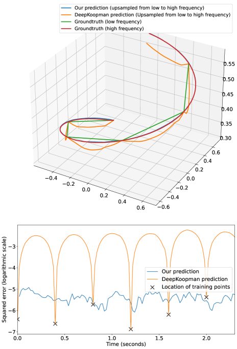
Figure 3: Upsampling experiment on fluid flow data. We learn a model on low-frequency data and then use the continuous representation to make a high-frequency prediction which we compare to the groundtruth. Top: our model and DeepKoopman compared to the groundtruth trajectory. Bottom: corresponding mean squared errors over time, in a logarithmic scale.

TABLE I: 50 Hz prediction of fluid flow dynamics with training data sampled at different frequencies

Training	DeepKoopman	Our method
sampling frequency	interpolation MSE	interpolation MSE
50 Hz	$\mathbf{1.21\times 10^{-6}}$	$1.65\times 10^{-6}$
25 Hz	$1.44\times 10^{-6}$	$\mathbf{1.11\times 10^{-6}}$
10 Hz	$1.36\times 10^{-5}$	$\mathbf{1.39\times 10^{-6}}$
5 Hz	$2.15\times 10^{-4}$	$\mathbf{1.62\times 10^{-6}}$
2.5 Hz	$2.31\times 10^{-3}$	$\mathbf{1.66\times 10^{-6}}$

IV-B Learning to predict forward and backward

Here, we investigate the ability of our models to perform backward predictions after being trained on forward prediction. In theory, one can simply invert the learnt matrix $\mathbf{K}$. This is not a possibility of the DeepKoopman framework since it computes a new matrix $\mathbf{K}$ as a function of the input at each iteration, and one would need to invert the matrix of the preceding state (which one does not have access to) to predict backwards. Table II reports our mean squared errors: in this table, ”HF” means that the model was trained on high-frequency data (50 Hz) while ”LF” means that it was trained on low-frequency data (2.5 Hz). One can see that the backward predictions have significantly higher errors in average than forward predictions. This matches the observation by [33] that naively inverting a learnt Koopman matrix is generally not effective. In particular, our model trained on low-frequency forecasting with no orthogonality term quickly diverges from the groundtruth when performing backward predictions. However, our model with an orthogonality regularisation trades reduced forecasting performances for the ability to run better backward reconstructions although it was not trained on this task. Figure 4 shows a typical example for which the model with an orthogonal matrix sticks to the time series while the unregularised one diverges from it.

As will be shown in subsequent experiments, the models trained with an orthogonality regularisation are more stable and versatile than their unregularised counterparts in general, making them more suitable for downstream tasks.

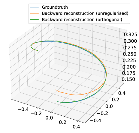
Figure 4: Backward reconstructions of a test time series from a model trained with an orthogonality loss term (orthogonal) and a model trained without it (unregularised). Both models were trained on high-frequency forecasting.

TABLE II: Mean squared errors for forward and backward predictions

Task \  Model	Unregularised	With orthogonality
Forward prediction (HF)	$\mathbf{1.65\times 10^{-6}}$	$5.50\times 10^{-6}$
Backward prediction (HF)	$1.88\times 10^{-4}$	$\mathbf{1.48\times 10^{-4}}$
Forward prediction (LF)	$\mathbf{1.66\times 10^{-6}}$	$8.89\times 10^{-6}$
Backward prediction (LF)	$0.123$	$\mathbf{3.24\times 10^{-5}}$

V Experiments on real Sentinel-2 time series

In this section, we work on multispectral satellite image time series. They consist in successive multivariate images of the forests of Fontainebleau and Orléans in France, which have been taken by the Sentinel-2 satellites as a part of the European Copernicus program [49] over a duration of nearly 5 years. We use the reflectance from $L=10$ visible and infrared spectral bands at a spatial resolution of 10 meters, resorting to bicubic interpolation for those that were originally at a 20 meter resolution. Although the satellites have a revisit time of five days, many images are unexploitable due to the presence of too many clouds between the satellite and the surface. Therefore, we performed temporal interpolation of the available data to obtain complete versions of the time series, along with the original incomplete versions for training on irregularly sampled data and assimilation purposes. The interpolation is performed with the Cressman method, which fills each missing value with a normalized sum of the available data, weighted by a gaussian function of the temporal distance to the filled time, with a gaussian radius of 15 days. We show RGB compositions of sample images from these time series in figure 5. Further details are available in [50], and the data is freely accessible from github.com/anthony-frion/Sentinel2TS. Throughout this section, the reported mean squared errors are averaged over all spectral bands, pixels and available times.

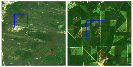
Figure 5: Left: a temporally interpolated Fontainebleau image. Right: a non- interpolated Orléans image. The date for both images is 20/06/2018. Those are RGB compositions with saturated colors. The red square is the $150\times 150$ pixel training area and the blue squares are test areas.

V-A Forecasting

First, we train a model to perform predictions from an initial condition on the 10-dimensional reflectance vector of a given pixel. Our encoder $\phi$ is a multi-layer perceptron with hidden layers of size 512 and 256, and the decoder $\psi$ has a symmetric architecture. The latent space and matrix $\mathbf{K}$ have a size of 32.

The model is trained on the interpolated version of the Fontainebleau dataset, containing 343 images, of which we use the first 243 for training and the last 100 for validation. Note that we do not train our model on 243-time-steps pixel reflectance time series but on time series of length 100 extracted from the data. In this way, our model learns to predict from any initial condition rather than just from the initial time of the dataset. Therefore, a trained model is able to model the long-term reflectance dynamics of a pixel from only 2 observations (because we use an augmented state as presented in equation (8)). However, one can obtain a much more accurate forecast by taking into account a higher number of observations for a given pixel. Namely, one can try to predict the future dynamics of a pixel given a time series representing its past behavior. We perform this task using the variational cost from equation (22), where the set $H$ of observed time indices contains all positive integers up to time $T_{train}=242$ (i.e. the training data). while the groundtruth time series prolongs the observations up to time index $T_{val}=342$. We investigate minimising this cost with no spatial regularisation or with a simple Tikhonov regularisation favoring the spatial smoothness of the resulting time series. More precisely, we seek to solve

$$\mathbf{z}_{0}^{*}=\underset{\mathbf{z}_{0}\in\mathbb{R}^{N\times d}}{\textrm{arg min}}\sum_{t=0}^{T_{train}}||\mathbf{\tilde{x}}_{t}-\mathbf{x}_{t}(\mathbf{z}_{0})||^{2}+\beta S(\mathbf{x}_{t}(\mathbf{z}_{0}))$$ (25)

where we again note $\mathbf{x}_{t}(\mathbf{z}_{0})=\psi(\mathbf{K}^{t}\mathbf{z}_{0})$, and $S(\mathbf{x})$ is a smoothness prior, penalizing the square of the spatial gradient of the resulting images through first order finite differences. The case with no spatial regularisation simply corresponds to $\beta=0$. Once $\mathbf{z}_{0}^{*}$ has been computed, one can use it to extend the generated time series at will by simply using higher powers of $\mathbf{K}$. We will refer to this technique as assimilation-forecasting. We solve this equation with gradient descent, using $\mathbf{z}_{0}=\phi(\tilde{\mathbf{x}}_{0})$ as a starting point, which is more effective than a random starting point. Should $\mathbf{z}_{0}^{*}$ be equal to $\phi(\tilde{\mathbf{x}}_{0})$, then this would be equivalent to simply performing a forecast from the initial state $\tilde{\mathbf{x}}_{0}$, which is not the case in practice. One can observe assimilation-forecasting results in a 3-dimensional PCA projection of a $100\times 100$ subcrop of the data in figure 6 and for a particular pixel in figure 7. Note that, even though all the pixels correspond to a forest environment, one can visually see that there are various long-term patterns among the pixels, and that our model can model them all.

We also try to forecast the Orléans time series in the same way with a model trained on the forest of Fontainebleau in order to test the zero-shot transfer performance of our model. Note that, in addition to being unseen during training, the Orléans data is irregularly sampled, which makes it harder to predict with assimilation-forecasting. All quantitative forecasting performances of our model are reported in table III, along with the performance of a long short-term memory network (LSTM) trained on the same Fontainebleau data. As previously mentioned, using assimilation-forecasting is far more effective than a simple prediction from an initial state. Using an additional smoothness prior further improves the results. One can also see that assimilation-forecasting achieves better results than an LSTM for long-term forecasting of this dataset, mainly because the LSTM is more fit to short-term prediction and tends to accumulate errors after multiple steps of nonlinear computation, as can be qualitatively assessed on figure 7. In many cases, the long-term predictions of the LSTM diverge in amplitude. In contrast, our model, being driven by a nearly orthogonal matrix, is very stable on the long-term and well fit for time series with a pseudo-periodic pattern.

Additionally, we noticed that training a model without the orthogonality loss term results in slightly better results for naive prediction from a given initial condition but far worse assimilation-forecasting results. This is in line with the results from section IV-B and confirms that the models with a nearly orthogonal matrix are better for performing downstream tasks.

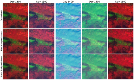
Figure 6: Top: groundtruth images of Fontainebleau, corresponding to test times. Middle: predictions made by our model by assimilating the time series up to day 1200 with a trained model. Bottom: Same as middle but including a spatial regularisation in the variational cost. The colors result from a 3-dimensional principal component analysis (PCA) of the 10 spectral bands performed globally on all the Fontainebleau data. This is much more informative than an RGB composition, mainly because vegetation is very reflective in the near-infrared domain.

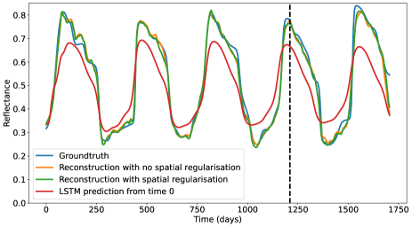
Figure 7: Predictions of different methods for the reflectance of the B7 band (in near infrared). The vertical line marks the limit between the training and the validation data. The pixel of interest is marked by a red dot on the Fontainebleau image from figure 5.

TABLE III: Forecasting MSE for different areas and methods

	Fontainebleau	Orléans (irregular data)
Prediction	$2.14\times 10^{-3}$	$8.90\times 10^{-3}$
from time 0
Assimilation-forecasting	$7.28\times 10^{-4}$	$3.94\times 10^{-3}$
Assimilation-forecasting	$\mathbf{7.08\times 10^{-4}}$	$\mathbf{3.75\times 10^{-3}}$
(with spatial prior)
LSTM from	$4.26\times 10^{-3}$	$1.38\times 10^{-2}$
time 0
LSTM from	$1.42\times 10^{-3}$	$6.80\times 10^{-3}$
time $T_{train}$

V-B Interpolation through data assimilation

We now move on to performing interpolation tasks. As previously mentioned, the satellite image time series are usually incomplete since most of the observations are too cloudy to be exploited. Therefore, one often has to interpolate them in time to work with regularly sampled data. Here, we perform variational data assimilation, using our data-based model to constrain the search. The variational cost, in the framework of equation (23), is minimised jointly on the latent initial condition and on the parameters of the pre-trained model.

Here, we test on raw incomplete data while our model was trained only on interpolated data from the forest of Fontainebleau. We consider the areas in the blue squares from figure 5. In both cases, we have at our disposal a set of around 85 $100\times 100\times 10$ images, each with its associated time index, irregularly sampled over a duration of 342 time steps (i.e. nearly 5 five years). From this set, we randomly mask half of the images which we use for the interpolation, while keeping the other half as a groundtruth to evaluate the quality of the computed interpolation. As a point of comparison, we seek the periodic pattern that best matches the available data, with a temporal smoothness prior using Tikhonov regularisation in the time dimension. Namely, we solve

$$\underset{\mathbf{x}\in\mathbb{R}^{p\times N\times L}}{\textrm{arg min}}\sum_{t\in H}||\tilde{\mathbf{x}}_{t}-\mathbf{x}_{t\%p}||^{2}+\alpha S_{t}(\mathbf{x}),$$ (26)

where $p$ is the known pseudo-period of one year, we use the notation $t\%p$ for the remainder of the Euclidean division of $t$ by $p$, and $S_{t}$ is the temporal smoothness prior. This method, which we call ”periodic interpolation”, is a strong baseline since it explicitly leverages the physical knowledge of the pseudo-period of the data. Yet, even if it was not trained on this data but only fine-tuned on it, our model has better results, as can be seen quantitatively in table IV and for a particular pixel of the forest of Orléans on figure 8. We show in the table the mean and standard deviation of the mean squared errors over 20 randomly computed masks.

Since the baseline method obtains much better results on Fontainebleau than on Orléans, the former seems to be easier to interpolate, yet the gap between this method and ours is bigger on this area since it is closer to the training data.

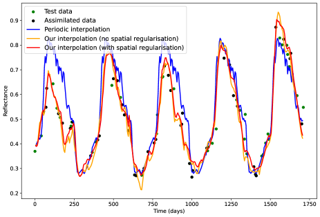
Figure 8: Comparison of interpolations for an Orléans pixel on the B7 band, using periodic interpolation and using data assimilation with our model trained on Fontainebleau data. We show an interpolation with no spatial regularisation (as can be found in [50]) and an interpolation with an additional spatial regularisation in the variational cost. The pixel of interest is marked by a red dot on the Orléans image on figure 5.

TABLE IV: Interpolation MSE ($\times 10^{-3}$) for different areas and methods

Periodic	Fontainebleau	Orléans
Periodic assimilation	$0.628\pm 0.128$	$2.37\pm 0.38$
Our method	$0.349\pm 0.154$	$2.22\pm 0.37$
Our method	$\mathbf{0.335\pm 0.146}$	$\mathbf{2.13\pm 0.34}$
(with spatial prior)

V-C Training on an irregular time series

As our final experiment, we investigate the training of our architecture on an irregular version of the Fontainebleau time series. This corresponds to the relatively simple setting mentioned in subsection III-B since this time series results from a regular sampling from which some observations have been removed because they were not usable. We were therefore able to optimise directly on the discrete operator $\mathbf{K}$ rather than on its continuous counterpart $\mathbf{L}$. As explained in subsection III-B, one just has to adapt the prediction, auto-encoding and linearity loss terms by computing them only for time delays for which the groundtruth is available. We were able to obtain satisfying results in this way, although the computed model is not as good as when training on interpolated time series. This tends to suggest that training our model directly on irregular time series can be a possibility when it is not possible to perform an interpolation as a pre-processing step.

We found that training on irregular data makes our model more subject to overfitting. Indeed, the model is not forced to predict a smooth evolution anymore but only to be able to correctly reconstruct some sparsely located points. Therefore, all regularisation terms that we presented in subsection III-A are very important to get the most out of this dataset. To support this claim, we performed an ablation study in which we tested different loss functions: the complete loss with the 4 terms from equations (9)-(12) and 4 versions where one of the terms has been removed. For each version of the loss function, we trained models on the Fontainebleau data from 5 different initialisations. We then retrieved the mean and standard deviations of the mean squared errors obtained when performing assimilation-forecasting as in subsection (V-A). The results are presented in table V. One can see that the final results on the Fontainebleau area largely depend on the model initialisation, yet both the mean and the standard deviation of the MSE are lower when using all loss terms.

TABLE V: Forecasting MSE ($\times 10^{-3}$) of models trained on irregularly-sampled data with different loss functions

	Fontainebleau	Orléans
Complete loss	$\mathbf{0.699\pm 0.130}$	$\mathbf{3.480\pm 0.198}$
No orthogonality	$0.922\pm 0.233$	$3.564\pm 0.301$
No linearity	$2.722\pm 0.576$	$5.454\pm 0.515$
No auto-encoding	$1.252\pm 0.128$	$3.770\pm 0.172$
No prediction	$3.514\pm 1.276$	$4.586\pm 0.232$

We show qualitative results of the assimilation-forecasting of irregular data using one of our models trained on irregular data with the complete loss function in figure 9. We emphasize that the blue curve is only a Cressman interpolation of the groundtruth points and should not be seen as a groundtruth here. Our model fits the training points well and, in some way, performs a smoother interpolation between those than the Cressman interpolation that was used to obtain the regularly-sampled data from section V-A.

We emphasize that, when tested on the same irregular test data, models trained on interpolated Fontainebleau data have better interpolation performance but lower forecasting performance than models trained on irregular Fontainebleau data. Using interpolation as a pre-processing step is not a trivial choice since models trained on these data will learn the interpolation scheme along with the true data. However, it can be seen as a form of data augmentation.

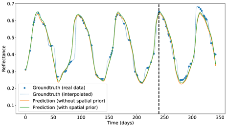
Figure 9: Forecasting results on the B7 band, with irregular data from the forest of Fontainebleau. The considered pixel is marked by a blue dot on figure 5.

VI Discussion

In the assimilation results presented in the previous section, adding a regularisation on the spatial gradient generally only results in a modest improvement of the mean squared error compared to using no regularisation. Since the chosen regularisation was a very basic one, this suggests that our predictions could gain more from spatial information. One could imagine using a more complex spatial prior, e.g. a data-driven one like in [39]. One could also use an image as the input of the Koopman auto-encoder instead of a single pixel, which would enable it to directly leverage spatial information (e.g. with a convolutional architecture) but might be more difficult and less suited to pixel-level downstream tasks. Another possibility is to train a convolutional neural network to correct the residual errors made when recomposing images from our pixelwise model. This approach has been presented in [50] and it can indeed improve the results. Yet, it is much less flexible and elegant since such a CNN needs to be trained for every new model or task considered, for which we do not necessarily have enough time or data.

The weights of the prior terms in assimilation should be chosen carefully, although a slightly inaccurate choice is unlikely to severely affect the results. A good way to proceed, when possible, is to use a set of validation data to set the parameters $\alpha$ and $\beta$ from equations (21)-(23). About the choice of allowing the parameters of the pretrained model to vary when performing data assimilation (i.e. solving the problem from equation (22) or (23)), it seems from our experiments that: (1) It is more beneficial to make the parameters vary when working with data that differ from what could be found in the training dataset. This can be seen as fine-tuning the model. (2) Allowing the model parameters to vary is effective when performing interpolation, but more dangerous for forecasting. An explanation could be that a slightly modified model keeps its tendency to generate smooth trajectories but not necessarily its long-term stability. One could investigate extensions of the framework of equation (23) with e.g. an orthogonality term to make sure that the modified model remains stable.

VII Conclusion

In this paper, we presented a method that enables to jointly learn a Koopman invariant subspace and an associated Koopman matrix of a dynamical system in a data-driven way. We showed that this method enables to learn a continuous representation of dynamical systems from discrete data, even in difficult contexts where the data are sparsely or irregularly sampled. In addition, it was demonstrated that a trained model is not only useful to forecast the future state of a dynamical system but also to solve downstream tasks. Indeed, we used the forward prediction as a pretext task to learn general useful information about the dynamical system in a self-supervised way. Since our architecture is fully differentiable, we showed how this information can be leveraged to solve inverse problems using variational data assimilation.

A possible extension of our work is to introduce a control variable in order to better predict the state of systems on which we know that some information is lacking. For example, precipitation data could be used as a control variable to better predict the vegetation reflectance. For image data specifically, one could make a better use of the spatial structure of the images by learning a complex spatial prior that would be coupled to the dynamical prior or by directly learning an end-to-end model that takes into account both dynamical and spatial information. Finally, a stochastic extension of our framework would make it able to output distributions of possible trajectories rather than single predictions.

Appendix A Using a (special) orthogonal matrix for the Koopman operator leads to periodic dynamics

Let us assume that we have found a KIS that leads us to consider linear Koopman dynamics in a latent space given by $\mathbf{z}_{t}\in\mathbb{R}^{d}$. Let us further assume the discrete dynamics are given by

$$\mathbf{z}_{t+1}=\mathbf{Kz}_{t}$$ (27)

where $\mathbf{K}\in\mathcal{SO}(d)$, i.e. $\mathbf{K}$ belongs to the special orthogonal group, i.e. the group of invertible matrices satisfying $\mathbf{KK}^{T}=\mathbf{K}^{T}\mathbf{K}=\mathbf{I}$, and with determinant equal to $+1$.

First we note that the norm of the iterates $\mathbf{z}_{t}$ remain equal to that of the initial condition $\mathbf{z}_{0}$. Indeed:

$$||\mathbf{z}_{t+1}||^{2}=||\mathbf{Kz}_{t}||^{2}=\mathbf{z}_{t}^{T}\mathbf{K}^{T}\mathbf{K}\mathbf{z}_{t}=\mathbf{z}_{t}^{T}\mathbf{z}_{t}=||\mathbf{z}_{t}||^{2}$$ (28)

and it is easy to see by induction that every iterate’s norm is equal to $||\mathbf{z}_{0}||$. So the dynamics remain on a sphere of radius $||\mathbf{z}_{0}||$.

Besides, $\mathcal{SO}(d)$ is a Lie group, whose Lie algebra $\mathfrak{so}(d)$ is the set of skew-symmetric matrices of size $d$. Furthermore, as $\mathcal{SO}(d)$ is compact, the exponential map $\exp:\mathfrak{so}(d)\to\mathcal{SO}(d)$, corresponding here to the matrix exponential, is surjective [51]. This means that any special orthogonal matrix can be written as the matrix exponential of a skew-symmetric matrix $\mathbf{L}$: $\exp(\mathbf{L})=\mathbf{K}$. Equivalently, a skew-symmetric matrix logarithm of a special orthogonal matrix always exists. In these conditions, we can see that $\mathbf{z}_{t+1}$ is the solution to the following ODE, representing the same dynamics in continuous time:

$$\frac{d\mathbf{z}}{dt}=\mathbf{Lz}$$ (29)

with $\mathbf{z}(0)=\mathbf{z}_{t}$. We proceed to show that the dynamics generated by this ODE must be periodic.

$\mathbf{L}$ is a skew-symmetric matrix, to which the spectral theorem applies: it can be diagonalized in a unitary basis, and its eigenvalues must be purely imaginary. There exists $\mathbf{U}\in\mathcal{U}(d)$ such that:

$$\mathbf{L}=\mathbf{U}^{*}\mathbf{D}\mathbf{U}$$ (30)

with $\mathbf{D}=\textrm{diag}(i\alpha_{1},i\alpha_{2},...,i\alpha_{d}),\alpha_{k}\in\mathbb{R}.$ By denoting $\mathbf{K}^{\tau}=\exp(\tau\mathbf{L})$ (giving $\mathbf{z}_{t}$ by matrix multiplication with $\mathbf{z}_{0}$), we can write:

$$\mathbf{K}^{\tau}=\exp(\tau\mathbf{L})=\mathbf{U}^{*}\exp(\tau\mathbf{D})\mathbf{U}$$ (31)

If we write out $\mathbf{K}^{\tau}_{rs}$, denoting as $\mathbf{u}_{r}$ the $r\textsuperscript{th}$ column of $\mathbf{U}$, we get

$$\mathbf{K}^{\tau}_{rs}=\mathbf{u}_{r}^{*}\exp(\tau\mathbf{D})\mathbf{u}_{s}=\sum_{k=1}^{d}u_{kr}^{*}\exp(i\tau\alpha_{k})u_{sk}.$$ (32)

The exponential factor is periodic of period $\frac{2\pi}{\alpha_{k}}$. Hence each entry of $\mathbf{K}^{\tau}$ is a linear combination of periodic functions. Mathematically, such a linear combination is only periodic when all the ratios between pairs of periods of the summands are rational. For all practical purposes, however, when numbers are represented with finite precision in a computer, such a linear combination can be itself seen as periodic. Finally, the same argument applies for the whole matrix $\mathbf{K}^{\tau}$ to be periodic.

This shows that the dynamics of linear dynamical system specified with a skew-symmetric matrix (when continuous) or with a special orthogonal matrix (when discrete) leads to periodic dynamics. Note that this property carries on to any time independent transformation of $\mathbf{z}_{t}$: for any regular enough function $\psi$, $\psi(\mathbf{z}(t))$ will itself be periodic with the same period as $\mathbf{z}(t)$.

References

- [1] M. Rußwurm, C. Pelletier, M. Zollner, S. Lefèvre, and M. Körner, “Breizhcrops: a time series dataset for crop type mapping,” ISPRS-International Archives of the Photogrammetry, Remote Sensing and Spatial Information Sciences, vol. 43, pp. 1545–1551, 2020.
- [2] G. Weikmann, C. Paris, and L. Bruzzone, “Timesen2crop: A million labeled samples dataset of Sentinel 2 image time series for crop-type classification,” IEEE J-STARS, vol. 14, pp. 4699–4708, 2021.
- [3] X. Liu, F. Zhang, Z. Hou, L. Mian, Z. Wang, J. Zhang, and J. Tang, “Self-supervised learning: Generative or contrastive,” IEEE Transactions on Knowledge and Data Engineering, vol. 35, no. 1, pp. 857–876, 2021.
- [4] C. Doersch, A. Gupta, and A. A. Efros, “Unsupervised visual representation learning by context prediction,” in IEEE ICCV, 2015, pp. 1422–1430.
- [5] S. Gidaris, P. Singh, and N. Komodakis, “Unsupervised representation learning by predicting image rotations,” in ICLR, 2018.
- [6] T. Chen, S. Kornblith, M. Norouzi, and G. Hinton, “A simple framework for contrastive learning of visual representations,” in ICML. PMLR, 2020, pp. 1597–1607.
- [7] Y. Wang, C. Albrecht, N. A. A. Braham, L. Mou, and X. Zhu, “Self-supervised learning in remote sensing: A review,” IEEE GRSM, 2022.
- [8] T. Brown, B. Mann, N. Ryder, M. Subbiah, J. D. Kaplan, P. Dhariwal, A. Neelakantan, P. Shyam, G. Sastry, A. Askell et al., “Language models are few-shot learners,” NeurIPS, vol. 33, pp. 1877–1901, 2020.
- [9] G. Evensen, F. C. Vossepoel, and P. J. van Leeuwen, Data assimilation fundamentals: A unified formulation of the state and parameter estimation problem. Springer Nature, 2022.
- [10] R. A. Borsoi, T. Imbiriba, P. Closas, J. C. M. Bermudez, and C. Richard, “Kalman filtering and expectation maximization for multitemporal spectral unmixing,” IEEE Geoscience and Remote Sensing Letters, vol. 19, pp. 1–5, 2020.
- [11] R. A. Borsoi, T. Imbiriba, and P. Closas, “Dynamical hyperspectral unmixing with variational recurrent neural networks,” IEEE TIP, 2023.
- [12] J. M. Lewis and J. C. Derber, “The use of adjoint equations to solve a variational adjustment problem with advective constraints,” Tellus A, vol. 37, no. 4, pp. 309–322, 1985.
- [13] M. Nonnenmacher and D. S. Greenberg, “Deep emulators for differentiation, forecasting, and parametrization in earth science simulators,” Journal of Advances in Modeling Earth Systems, vol. 13, no. 7, p. e2021MS002554, 2021.
- [14] A. Paszke, S. Gross, S. Chintala, G. Chanan, E. Yang, Z. DeVito, Z. Lin, A. Desmaison, L. Antiga, and A. Lerer, “Automatic differentiation in pytorch,” 2017.
- [15] B. O. Koopman, “Hamiltonian systems and transformation in Hilbert space,” Proceedings of the National Academy of Sciences, vol. 17, no. 5, pp. 315–318, 1931.
- [16] S. L. Brunton, M. Budišić, E. Kaiser, and J. N. Kutz, “Modern Koopman theory for dynamical systems,” arXiv preprint arXiv:2102.12086, 2021.
- [17] A. Frion, L. Drumetz, M. Dalla Mura, G. Tochon, and A. Aïssa-El-Bey, “Leveraging neural Koopman operators to learn continuous representations of dynamical systems from scarce data,” in ICASSP. IEEE, 2023, pp. 1–5.
- [18] P. J. Schmid, “Dynamic mode decomposition of numerical and experimental data,” Journal of fluid mechanics, vol. 656, pp. 5–28, 2010.
- [19] C. W. Rowley, I. Mezić, S. Bagheri, P. Schlatter, and D. S. Henningson, “Spectral analysis of nonlinear flows,” Journal of fluid mechanics, vol. 641, pp. 115–127, 2009.
- [20] K. K. Chen, J. H. Tu, and C. W. Rowley, “Variants of dynamic mode decomposition: boundary condition, Koopman, and Fourier analyses,” Journal of nonlinear science, vol. 22, pp. 887–915, 2012.
- [21] J. H. Tu, C. W. Rowley, D. M. Luchtenburg, S. L. Brunton, and J. N. Kutz, “On dynamic mode decomposition: Theory and applications,” Journal of Computational Dynamics, vol. 1, no. 2, pp. 391–421, 2014.
- [22] J. N. Kutz, X. Fu, and S. L. Brunton, “Multiresolution dynamic mode decomposition,” SIAM Journal on Applied Dynamical Systems, vol. 15, no. 2, pp. 713–735, 2016.
- [23] M. O. Williams, I. G. Kevrekidis, and C. W. Rowley, “A data–driven approximation of the Koopman operator: Extending dynamic mode decomposition,” Journal of Nonlinear Science, vol. 25, pp. 1307–1346, 2015.
- [24] Y. Kawahara, “Dynamic mode decomposition with reproducing kernels for Koopman spectral analysis,” NeurIPS, vol. 29, 2016.
- [25] V. Kostic, P. Novelli, A. Maurer, C. Ciliberto, L. Rosasco, and M. Pontil, “Learning dynamical systems via Koopman operator regression in reproducing kernel Hilbert spaces,” NeurIPS, vol. 35, pp. 4017–4031, 2022.
- [26] P. Bevanda, M. Beier, A. Lederer, S. Sosnowski, E. Hüllermeier, and S. Hirche, “Koopman kernel regression,” arXiv:2305.16215, 2023.
- [27] Q. Li, F. Dietrich, E. M. Bollt, and I. G. Kevrekidis, “Extended dynamic mode decomposition with dictionary learning: A data-driven adaptive spectral decomposition of the Koopman operator,” Chaos: An Interdisciplinary Journal of Nonlinear Science, vol. 27, no. 10, p. 103111, 2017.
- [28] E. Yeung, S. Kundu, and N. Hodas, “Learning deep neural network representations for Koopman operators of nonlinear dynamical systems,” in American Control Conference (ACC). IEEE, 2019, pp. 4832–4839.
- [29] B. Lusch, J. N. Kutz, and S. L. Brunton, “Deep learning for universal linear embeddings of nonlinear dynamics,” Nature communications, vol. 9, no. 1, p. 4950, 2018.
- [30] S. E. Otto and C. W. Rowley, “Linearly recurrent autoencoder networks for learning dynamics,” SIAM Journal on Applied Dynamical Systems, vol. 18, no. 1, pp. 558–593, 2019.
- [31] J. Morton, A. Jameson, M. J. Kochenderfer, and F. Witherden, “Deep dynamical modeling and control of unsteady fluid flows,” NeurIPS, vol. 31, 2018.
- [32] Y. Li, H. He, J. Wu, D. Katabi, and A. Torralba, “Learning compositional Koopman operators for model-based control,” in ICLR, 2019.
- [33] O. Azencot, N. B. Erichson, V. Lin, and M. Mahoney, “Forecasting sequential data using consistent Koopman autoencoders,” in ICML. PMLR, 2020, pp. 475–485.
- [34] K. He, X. Zhang, S. Ren, and J. Sun, “Deep residual learning for image recognition,” in IEEE CVPR, 2016, pp. 770–778.
- [35] A. Saxe, J. McClelland, and S. Ganguli, “Exact solutions to the nonlinear dynamics of learning in deep linear neural networks,” in ICLR, 2014.
- [36] D. Xie, J. Xiong, and S. Pu, “All you need is beyond a good init: Exploring better solution for training extremely deep convolutional neural networks with orthonormality and modulation,” in IEEE CVPR, 2017, pp. 6176–6185.
- [37] A. Krogh and J. Hertz, “A simple weight decay can improve generalization,” NeurIPS, vol. 4, 1991.
- [38] N. Bansal, X. Chen, and Z. Wang, “Can we gain more from orthogonality regularizations in training deep networks?” NeurIPS, vol. 31, 2018.
- [39] R. Fablet, L. Drumetz, and F. Rousseau, “Joint learning of variational representations and solvers for inverse problems with partially-observed data,” arXiv:2006.03653, 2020.
- [40] A. Farchi, P. Laloyaux, M. Bonavita, and M. Bocquet, “Using machine learning to correct model error in data assimilation and forecast applications,” Quarterly Journal of the Royal Meteorological Society, vol. 147, no. 739, pp. 3067–3084, 2021.
- [41] S. Cheng et al., “Machine learning with data assimilation and uncertainty quantification for dynamical systems: a review,” arXiv:2303.10462, 2023.
- [42] F. Takens, “Detecting strange attractors in turbulence,” in Dynamical Systems and Turbulence: proceedings of a symposium held at the University of Warwick 1979/80. Springer, 2006, pp. 366–381.
- [43] W. J. Culver, “On the existence and uniqueness of the real logarithm of a matrix,” Proceedings of the American Mathematical Society, vol. 17, no. 5, pp. 1146–1151, 1966.
- [44] R. A. Willoughby, “Solutions of Ill-Posed Problems (A. N. Tikhonov and V. Y. Arsenin),” SIAM Review, vol. 21, no. 2, pp. 266–267, 1979.
- [45] L. I. Rudin, S. Osher, and E. Fatemi, “Nonlinear total variation based noise removal algorithms,” Physica D: nonlinear phenomena, vol. 60, no. 1-4, pp. 259–268, 1992.
- [46] J. Kirkpatrick et al., “Overcoming catastrophic forgetting in neural networks,” PNAS, vol. 114, no. 13, pp. 3521–3526, 2017.
- [47] C. Sun, X. Qiu, Y. Xu, and X. Huang, “How to fine-tune BERT for text classification?” in Chinese Computational Linguistics: 18th China National Conference, CCL 2019, Kunming, China, October 18–20, 2019, Proceedings 18. Springer, 2019, pp. 194–206.
- [48] B. R. Noack, K. Afanasiev, M. Morzyński, G. Tadmor, and F. Thiele, “A hierarchy of low-dimensional models for the transient and post-transient cylinder wake,” Journal of Fluid Mechanics, vol. 497, pp. 335–363, 2003.
- [49] S. Jutz and M. Milagro-Pérez, “Copernicus: the european Earth observation programme,” Revista de Teledetección, no. 56, pp. V–XI, 2020.
- [50] A. Frion, L. Drumetz, G. Tochon, M. D. Mura, and A. A. E. Bey, “Learning Sentinel-2 reflectance dynamics for data-driven assimilation and forecasting,” in EUSIPCO 2023, 2023, pp. 1–5.
- [51] T. Bröcker and T. Tom Dieck, Representations of compact Lie groups. Springer Science & Business Media, 2013, vol. 98.