Two-way Linear Probing Revisited
Abstract. We introduce linear probing hashing schemes that construct a hash table of size , with constant load factor , on which the worst-case unsuccessful search time is asymptotically almost surely . The schemes employ two linear probe sequences to find empty cells for the keys. Matching lower bounds on the maximum cluster size produced by any algorithm that uses two linear probe sequences are obtained as well.
Categories and Subject Descriptors: E.2 [Data]: Data Storage Representa-tions—hash-table representations; F.2.2 [Analysis of Algorithms and Problem Complexity]: Non-numerical Algorithms and Problems—sorting and searching
General Terms: Algorithms, Theory
Additional Keywords and Phrases: Open addressing hashing, linear probing, parking problem, worst-case search time, two-way chaining, multiple-choice paradigm, randomized algorithms, witness tree, probabilistic analysis.
1 Introduction
In classical open addressing hashing [75], keys are hashed sequentially and on-line into a table of size , (that is, a one-dimensional array with cells which we denote by the set ), where each cell can harbor at most one key. Each key has only one infinite probe sequence , for . During the insertion process, if a key is mapped to a cell that is already occupied by another key, a collision occurs, and another probe is required. The probing continues until an empty cell is reached where a key is placed. This method of hashing is pointer-free, unlike hashing with separate chaining where keys colliding in the same cell are hashed to a separate linked list or chain. For a discussion of different hashing schemes see [41, 51, 92].
The purpose of this paper is to design efficient open addressing hashing schemes that improve the worst-case performance of classical linear probing where , for . Linear probing is known for its good practical performance, efficiency, and simplicity. It continues to be one of the best hash tables in practice due to its simplicity of implementation, absence of overhead for internally used pointers, cache efficiency, and locality of reference [46, 73, 81, 88]. On the other hand, the performance of linear probing seems to degrade with high load factors , due to a primary-clustering tendency of one collision to cause more nearby collisions.
Our study concentrates on schemes that use two linear probe sequences to find possible hashing cells for the keys. Each key chooses two initial cells independently and uniformly at random, with replacement. From each initial cell, we probe linearly, and cyclically whenever the last cell in the table is reached, to find two empty cells which we call terminal cells. The key then is inserted into one of these terminal cells according to a fixed strategy. We consider strategies that utilize the greedy multiple-choice paradigm [5, 93]. We show that some of the trivial insertion strategies with two-way linear probing have unexpected poor performance. For example, one of the trivial strategies we study inserts each key into the terminal cell found by the shorter probe sequence. Another simple strategy inserts each key into the terminal cell that is adjacent to the smaller cluster, where a cluster is an isolated set of consecutively occupied cells. Unfortunately, the performances of these two strategies are not ideal. We prove that when any of these two strategies is used to construct a hash table with constant load factor, the maximum unsuccessful search time is , with high probability (w.h.p.). Indeed, we prove that, w.h.p., a giant cluster of size emerges in a hash table of constant load factor, if it is constructed by a two-way linear probing insertion strategy that always inserts any key upon arrival into the empty cell of its two initial cells whenever one of them is empty.
Consequently, we introduce two other strategies that overcome this problem. First, we partition the hash table into equal-sized blocks of size , assuming is an integer. We consider the following strategies for inserting the keys:
-
A.
Each key is inserted into the terminal cell that belongs to the least crowded block, i.e., the block with the least number of keys.
-
B.
For each block , we define its weight to be the number of keys inserted into terminal cells found by linear probe sequences whose starting locations belong to block . Each key, then, is inserted into the terminal cell found by the linear probe sequence that has started from the block of smaller weight.
For strategy B, we show that can be chosen such that for any constant load factor , the maximum unsuccessful search time is not more than , w.h.p., where is a function of . If , the same property also holds for strategy A. Furthermore, these schemes are optimal up to a constant factor in the sense that an universal lower bound holds for any strategy that uses two linear probe sequences, even if the initial cells are chosen according to arbitrary probability distributions.
For hashing with separate chaining, one can achieve maximum search time by applying the two-way chaining scheme [5] where each key is inserted into the shorter chain among two chains chosen independently and uniformly at random, with replacement, breaking ties randomly. It is proved [5, 8] that when keys are inserted into a hash table with chains, the length of the longest chain upon termination is , w.h.p. Of course, this idea can be generalized to open addressing. Assuming the hash table is partitioned into blocks of size , we allow each key to choose two initial cells, and hence two blocks, independently and uniformly at random, with replacement. From each initial cell and within its block, we probe linearly and cyclically, if necessary, to find two empty cells; that is, whenever we reach the last cell in the block and it is occupied, we continue probing from the first cell in the same block. The key, then, is inserted into the empty cell that belongs to the least full block. Using the two-way chaining result, one can show that for suitably chosen , the maximum unsuccessful search time is , w.h.p. However, this scheme uses probe sequences that are not totally linear; they are locally linear within the blocks.
1.1 History and Motivation
Probing and Replacement
Open addressing schemes are determined by the type of the probe sequence, and the replacement strategy for resolving the collisions. Some of the commonly used probe sequences are:
-
1.
Random Probing [67]: For every key , the infinite sequence is assumed to be independent and uniformly distributed over . That is, we require to have an infinite sequence of truly uniform and independent hash functions. If for each key , the first probes of the sequence are distinct, i.e., it is a random permutation, then it is called uniform probing [75].
-
2.
Linear Probing [75]: For every key , the first probe is assumed to be uniform on , and the next probes are defined by , for . So we only require to be a truly uniform hash function.
-
3.
Double Probing [6]: For every key , the first probe is , and the next probes are defined by , for , where and are truly uniform and independent hash functions.
Random and uniform probings are, in some sense, the idealized models [89, 97], and their plausible performances are among the easiest to analyze; but obviously they are unrealistic. Linear probing is perhaps the simplest to implement, but it behaves badly when the table is almost full. Double probing can be seen as a compromise.
During the insertion process of a key , suppose that we arrive at the cell which is already occupied by another previously inserted key , that is, , for some . Then a replacement strategy for resolving the collision is needed. Three strategies have been suggested in the literature (see [68] for other methods):
Average Performance
Evidently, the performance of any open addressing scheme deteriorates when the ratio approaches 1, as the cluster sizes increase, where a cluster is an isolated set of consecutively occupied cells (cyclically defined) that are bounded by empty cells. Therefore, we shall assume that the hash table is -full, that is, the number of hashed keys , where is a constant called the load factor. The asymptotic average-case performance has been extensively analyzed for random and uniform probing [9, 55, 67, 75, 89, 97], linear probing [50, 51, 54, 61], and double probing [6, 43, 57, 84, 86]. The expected search times were proven to be constants, more or less, depending on only. Recent results about the average-case performance of linear probing, and the limit distribution of the construction time have appeared in [32, 52, 91]. See also [3, 39, 76] for the average-case analysis of linear probing for nonuniform hash functions.
It is worth noting that the average search time of linear probing is independent of the replacement strategy; see [51, 75]. This is because the insertion of any order of the keys results in the same set of occupied cells, i.e., the cluster sizes are the same; and hence, the total displacement of the keys—from their initial hashing locations—remains unchanged. It is not difficult to see that this independence is also true for random and double probings. That is, the replacement strategy does not have any effect on the average successful search time in any of the above probings. In addition, since in linear probing the unsuccessful search time is related to the cluster sizes (unlike random and double probings), the expected and the maximum unsuccessful search times in linear probing are invariant to the replacement strategy.
Worst-case Performance
The focal point of this article, however, is the worst-case search time which is proportional to the length of the longest probe sequence over all keys (llps, for short). Many results have been established regarding the worst-case performance of open addressing.
The worst-case performance of linear probing with fcfs policy was analyzed by Pittel [77]. He proved that the maximum cluster size, and hence the llps needed to insert (or search for) a key, is asymptotic to , in probability. As we mentioned above, this bound holds for linear probing with any replacement strategy. Chassaing and Louchard [15] studied the threshold of emergence of a giant cluster in linear probing. They showed that when the number of keys , the size of the largest cluster is , w.h.p.; however, when , a giant cluster of size emerges, w.h.p.
Gonnet [40] proved that with uniform probing and fcfs replacement strategy, the expected llps is asymptotic to , for -full tables. However, Poblete and Munro [78, 79] showed that if random probing is combined with lcfs policy, then the expected llps is at most , where is the gamma function.
On the other hand, the robin hood strategy with random probing leads to a more striking performance. Celis [13] first proved that the expected llps is . However, Devroye, Morin and Viola [22] tightened the bounds and revealed that the llps is indeed , w.h.p., thus achieving a double logarithmic worst-case insertion and search times for the first time in open addressing hashing. Unfortunately, one cannot ignore the assumption in random probing about the availability of an infinite collection of hash functions that are sufficiently independent and behave like truly uniform hash functions in practice. On the other side of the spectrum, we already know that robin hood policy does not affect the maximum unsuccessful search time in linear probing. However, robin hood may be promising with double probing.
Other Initiatives
Open addressing methods that rely on rearrangement of keys were under investigation for many years, see, e.g., [10, 42, 58, 60, 68, 82]. Pagh and Rodler [74] studied a scheme called cuckoo hashing that exploits the lcfs replacement policy. It uses two hash tables of size , for some constant ; and two independent hash functions chosen from an -universal class—one function only for each table. Each key is hashed initially by the first function to a cell in the first table. If the cell is full, then the new key is inserted there anyway, and the old key is kicked out to the second table to be hashed by the second function. The same rule is applied in the second table. Keys are moved back and forth until a key moves to an empty location or a limit has been reached. If the limit is reached, new independent hash functions are chosen, and the tables are rehashed. The worst-case search time is at most two, and the amortized expected insertion time, nonetheless, is constant. However, this scheme utilizes less than 50% of the allocated memory, has a worst-case insertion time of , w.h.p., and depends on a wealthy source of provably good independent hash functions for the rehashing process. For further details see [21, 26, 33, 70].
The space efficiency of cuckoo hashing is significantly improved when the hash table is divided into blocks of fixed size and more hash functions are used to choose blocks for each key where each is inserted into a cell in one of its chosen blocks using the cuckoo random walk insertion method [25, 37, 34, 35, 56, 95]. For example, it is known [25, 56] that 89.7% space utilization can be achieved when and the hash table is partitioned into non-overlapping blocks of size . On the other hand, when the blocks are allowed to overlap, the space utilization improves to 96.5% [56, 95]. The worst-case insertion time of this generalized cuckoo hashing scheme, however, is proven [35, 38] to be polylogarithmic, w.h.p.
Many real-time static and dynamic perfect hashing schemes achieving constant worst-case search time, and linear (in the table size) construction time and space were designed in [11, 23, 24, 27, 28, 36, 71, 72]. All of these schemes, which are based, more or less, on the idea of multilevel hashing, employ more than a constant number of perfect hash functions chosen from an efficient universal class. Some of them even use functions.
1.2 Our Contribution
We design linear probing algorithms that accomplish double logarithmic worst-case search time. Inspired by the two-way chaining algorithm [5], and its powerful performance, we promote the concept of open addressing hashing with two-way linear probing. The essence of the proposed concept is based on the idea of allowing each key to generate two independent linear probe sequences and making the algorithm decide, according to some strategy, at the end of which sequence the key should be inserted. Formally, each input key chooses two cells independently and uniformly at random, with replacement. We call these cells the initial hashing cells available for . From each initial hashing cell, we start a linear probe sequence (with fcfs policy) to find an empty cell where we stop. Thus, we end up with two unoccupied cells. We call these cells the terminal hashing cells. The question now is: into which terminal cell should we insert the key ?
The insertion process of a two-way linear probing algorithm could follow one of the strategies we mentioned earlier: it may insert the key at the end of the shorter probe sequence, or into the terminal cell that is adjacent to the smaller cluster. Others may make an insertion decision even before linear probing starts. In any of these algorithms, the searching process for any key is basically the same: just start probing in both sequences alternately, until the key is found, or the two empty cells at the end of the sequences are reached in the case of an unsuccessful search. Thus, the maximum unsuccessful search time is at most twice the size of the largest cluster plus two.
We study the two-way linear probing algorithms stated above, and show that the hash table, asymptotically and almost surely, contains a giant cluster of size . Indeed, we prove that a cluster of size emerges, asymptotically and almost surely, in any hash table of constant load factor that is constructed by a two-way linear probing algorithm that inserts any key upon arrival into the empty cell of its two initial cells whenever one of them is empty.
We introduce two other two-way linear probing heuristics that lead to maximum unsuccessful search times. The common idea of these heuristics is the marriage between the two-way linear probing concept and a technique we call blocking where the hash table is partitioned into equal-sized blocks. These blocks are used by the algorithm to obtain some information about the keys allocation. The information is used to make better decisions about where the keys should be inserted, and hence, lead to a more even distribution of the keys.
Two-way linear probing hashing has several advantages over other proposed hashing methods, mentioned above: it reduces the worst-case behavior of hashing, it requires only two hash functions, it is easy to parallelize, it is pointer-free and easy to implement, and unlike the hashing schemes proposed in [25, 74], it does not require any rearrangement of keys or rehashing. Its maximum cluster size is , and its average-case performance can be at most twice the classical linear probing as shown in the simulation results. Furthermore, it is not necessary to employ perfectly random hash functions as it is known [73, 81, 88] that hash functions with smaller degree of universality will be sufficient to implement linear probing schemes. See also [27, 49, 70, 74, 84, 85, 86] for other suggestions on practical hash functions.
Paper Scope
In the next section, we recall some of the useful results about the greedy multiple-choice paradigm. We prove, in Section 3, a universal lower bound of order of on the maximum unsuccessful search time of any two-way linear probing algorithm. We prove, in addition, that not every two-way linear probing scheme behaves efficiently. We devote Section 4 to the positive results, where we present our two two-way linear probing heuristics that accomplish worst-case unsuccessful search time. Simulation results of the studied algorithms are summarized in Section 5.
Throughout, we assume the following. We are given keys—from a universe set of keys —to be hashed into a hash table of size such that each cell contains at most one key. The process of hashing is sequential and on-line, that is, we never know anything about the future keys. The constant is preserved in this article for the load factor of the hash table, that is, we assume that . The cells of the hash table are numbered . The linear probe sequences always move cyclically from left to right of the hash table. The replacement strategy of all of the introduced algorithms is fcfs. The insertion time is defined to be the number of probes the algorithm performs to insert a key. Similarly, the search time is defined to be the number of probes needed to find a key, or two empty cells in the case of unsuccessful search. Observe that unlike classical linear probing, the insertion time of two-way linear probing may not be equal to the successful search time. However, they are both bounded by the unsuccessful search time. Notice also that we ignore the time to compute the hash functions.
2 The Multiple-choice Paradigm
Allocating balls into bins is one of the historical assignment problems [48, 53]. We are given balls that have to be placed into bins. The balls have to be inserted sequentially and on-line, that is, each ball is assigned upon arrival without knowing anything about the future coming balls. The load of a bin is defined to be the number of balls it contains. We would like to design an allocation process that minimizes the maximum load among all bins upon termination. For example, in a classical allocation process, each ball is placed into a bin chosen independently and uniformly at random, with replacement. It is known [40, 63, 80] that if , the maximum load upon termination is asymptotic to , in probability.
On the other hand, the greedy multiple-choice allocation process, appeared in [30, 49] and studied by Azar et al. [5], inserts each ball into the least loaded bin among bins chosen independently and uniformly at random, with replacement, breaking ties randomly. Throughout, we will refer to this process by GreedyMC for inserting balls into bins. Surprisingly, the maximum bin load of GreedyMC decreases exponentially to , w.h.p., [5]. However, one can easily generalize this to the case . It is also known that the greedy strategy is stochastically optimal in the following sense.
Theorem 1 (Azar et al. [5]).
Let , where , and . Upon termination of GreedyMC, the maximum bin load is , w.h.p. Furthermore, the maximum bin load of any on-line allocation process that inserts balls sequentially into bins where each ball is inserted into a bin among bins chosen independently and uniformly at random, with replacement, is at least , w.h.p.
Berenbrink et al. [8] extended Theorem 1 to the heavily loaded case where , and recorded the following tight result.
Theorem 2 (Berenbrink et al. [8]).
There is a constant such that for any integers , and , the maximum bin load upon termination of the process GreedyMC is , w.h.p.
Theorem 2 is a crucial result that we have used to derive our results, see Theorems 8 and 9. It states that the deviation from the average bin load which is stays unchanged as the number of balls increases.
Vöcking [93, 94] demonstrated that it is possible to improve the performance of the greedy process, if non-uniform distributions on the bins and a tie-breaking rule are carefully chosen. He suggested the following variant which is called Always-Go-Left. The bins are numbered from 1 to . We partition the bins into groups of almost equal size, that is, each group has size . We allow each ball to select upon arrival bins independently at random, but the -th bin must be chosen uniformly from the -th group. Each ball is placed on-line, as before, in the least full bin, but upon a tie, the ball is always placed in the leftmost bin among the bins. We shall write LeftMC to refer to this process. Vöcking [93] showed that if , the maximum load of LeftMC is , w.h.p., where is a constant related to a generalized Fibonacci sequence. For example, the constant corresponds to the well-known golden ratio, and . In general, , and . Observe the improvement on the performance of GreedyMc, even for . The maximum load of LeftMC is , whereas in GreedyMC, it is . The process LeftMC is also optimal in the following sense.
Theorem 3 (Vöcking [93]).
Let , where , and . The maximum bin load of of LeftMC upon termination is , w.h.p. Moreover, the maximum bin load of any on-line allocation process that inserts balls sequentially into bins where each ball is placed into a bin among bins chosen according to arbitrary, not necessarily independent, probability distributions defined on the bins is at least , w.h.p.
Berenbrink et al. [8] studied the heavily loaded case and recorded the following theorem.
Theorem 4 (Berenbrink et al. [8]).
There is a constant such that for any integers , and , the maximum bin load upon termination of the process LeftMC is , w.h.p.
3 Life is not Always Good!
We prove here that the idea of two-way linear probing alone is not always sufficient to pull off a plausible hashing performance. We prove that a large group of two-way linear probing algorithms have an lower bound on their worst-case search time. To avoid any ambiguity, we consider this definition.
Definition 1.
A two-way linear probing algorithm is an open addressing hashing algorithm that inserts keys into cells using a certain strategy and does the following upon the arrival of each key:
-
1.
It chooses two initial hashing cells independently and uniformly at random, with replacement.
-
2.
Two terminal (empty) cells are then found by linear probe sequences starting from the initial cells.
-
3.
The key is inserted into one of these terminal cells.
To be clear, we give two examples of inefficient two-way linear probing algorithms. Our first algorithm places each key into the terminal cell discovered by the shorter probe sequence. More precisely, once the key chooses its initial hashing cells, we start two linear probe sequences. We proceed, sequentially and alternately, one probe from each sequence until we find an empty (terminal) cell where we insert the key. Formally, let be independent and truly uniform hash functions. For , define the linear sequence , and , for ; and similarly define the sequence . The algorithm, then, inserts each key into the first unoccupied cell in the following probe sequence: . We denote this algorithm that hashes keys into cells by ShortSeq, for the shorter sequence.
The second algorithm inserts each key into the empty (terminal) cell that is the right neighbor of the smaller cluster among the two clusters containing the initial hashing cells, breaking ties randomly. If one of the initial cells is empty, then the key is inserted into it, and if both of the initial cells are empty, we break ties evenly. Recall that a cluster is a group of consecutively occupied cells whose left and right neighbors are empty cells. This means that one can compute the size of the cluster that contains an initial hashing cell by running two linear probe sequences in opposite directions starting from the initial cell and going to the empty cells at the boundaries. So practically, the algorithm uses four linear probe sequences. We refer to this algorithm by SmallCluster for inserting keys into cells.
Before we show that these algorithms produce large clusters, we shall record a lower bound that holds for any two-way linear probing algorithm.
3.1 Universal Lower Bound
The following lower bound holds for any two-way linear probing hashing scheme, in particular, the ones that are presented in this article.
Theorem 5.
Let , and , where is a constant. Let be any two-way linear probing algorithm that inserts keys into a hash table of size . Then upon termination of , w.h.p., the table contains a cluster of size of at least .
Proof.
Imagine that we have a bin associated with each cell in the hash table. Recall that for each key , algorithm chooses two initial cells, and hence two bins, independently and uniformly at random, with replacement. Algorithm , then, probes linearly to find two (possibly identical) terminal cells, and inserts the key into one of them. Now imagine that after the insertion of each key , we also insert a ball into the bin associated with the initial cell from which the algorithm started probing to reach the terminal cell into which the key was placed. If both of the initial cells lead to the same terminal cell, then we break the tie randomly. Clearly, if there is a bin with balls, then there is a cluster of size of at least , because the balls represent distinct keys that belong to the same cluster. However, Theorem 1 asserts that the maximum bin load upon termination of algorithm is at least , w.h.p. ∎
The above lower bound is valid for all algorithms that satisfy Definition 1. A more general lower bound can be established on all open addressing schemes that use two linear probe sequences where the initial hashing cells are chosen according to some (not necessarily uniform or independent) probability distributions defined on the cells. We still assume that the probe sequences are used to find two (empty) terminal hashing cells, and the key is inserted into one of them according to some strategy. We call such schemes nonuniform two-way linear probing. The proof of the following theorem is basically similar to Theorem 5, but by using instead Vöcking’s lower bound as stated in Theorem 3.
Theorem 6.
Let , and , where is a constant. Let be any nonuniform two-way linear probing algorithm that inserts keys into a hash table of size where the initial hashing cells are chosen according to some probability distributions. Then the maximum cluster size produced by , upon termination, is at least , w.h.p.
3.2 Algorithms that Behave Poorly
We characterize some of the inefficient two-way linear probing algorithms. Notice that the main mistake in algorithms ShortSeq and SmallCluster is that the keys are allowed to be inserted into empty cells even if these cells are very close to some giant clusters. This leads us to the following theorem.
Theorem 7.
Let be constant. Let be a two-way linear probing algorithm that inserts keys into cells such that whenever a key chooses an empty and an occupied initial cells, the algorithm inserts the key into the empty one. Then algorithm produces a giant cluster of size , w.h.p.
To prove the theorem, we need to recall the following.
Definition 2 (See, e.g., [29]).
Any non-negative random variables are said to be negatively associated, if for every disjoint index subsets , and for any functions , and that are both non-decreasing or both non-increasing (componentwise), we have
Once we establish that are negatively associated, it follows, by considering inductively the indicator functions, that
The next lemmas, which are proved in [29, 31, 47], provide some tools for establishing the negative association.
Lemma 1 (Zero-One Lemma).
Any binary random variables whose sum is one are negatively associated.
Lemma 2.
If and are independent sets of negatively associated random variables, then the union is also a set of negatively associated random variables.
Lemma 3.
Suppose that are negatively associated. Let be disjoint index subsets, for some positive integer . For , let be non-decreasing functions, and define . Then the random variables are negatively associated. In other words, non-decreasing functions of disjoint subsets of negatively associated random variables are also negatively associated. The same holds if are non-increasing functions.
Throughout, we write to denote a binomial random variable with parameters and .
Proof of Theorem 7.
Let for some positive constants and to be defined later, and without loss of generality, assume that is an integer. Suppose that the hash table is divided into disjoint blocks, each of size . For , let be the set of cells of the -th block, where we consider the cell numbers in a circular fashion. We say that a cell is “covered” if there is a key whose first initial hashing cell is the cell and its second initial hashing cell is an occupied cell. A block is covered if all of its cells are covered. Observe that if a block is covered then it is fully occupied. Thus, it suffices to show that there would be a covered block, w.h.p.
For , let be the indicator that the -th block is covered. The random variables are negatively associated which can been seen as follows. For and , let be the indicator that the -th cell is covered by the -th key, and set . Notice that the random variable is binary. The zero-one Lemma asserts that the binary random variables are negatively associated. However, since the keys choose their initial hashing cells independently, the random variables are mutually independent from the random variables , for any distinct . Thus, by Lemma 2, the union is a set of negatively associated random variables. The negative association of the is assured now by Lemma 3 as they can be written as non-decreasing functions of disjoint subsets of the indicators . Since the are negatively associated and identically distributed, then
Thus, we only need to show that tends to infinity as goes to infinity. To bound the last probability, we need to focus on the way the first block is covered. For , let be the smallest such that (if such exists), and otherwise. We say that the first block is “covered in order” if and only if . Since there are orderings of the cells in which they can be covered (for the first time), we have
For , let if block is full before the insertion of the -th key, and otherwise be the minimum such that the cell has not been covered yet. Let be the event that, for all , the first initial hashing cell of the -th key is either cell or a cell outside . Define the random variable , where is the indicator that the -th key covers a cell in . Clearly, if is true and , then the first block is covered in order. Thus,
However, since the initial hashing cells are chosen independently and uniformly at random, then for chosen large enough, we have
and for ,
Therefore, for sufficiently large, we get
which goes to infinity as approaches infinity whenever and is any
positive constant less than 1.
Clearly, algorithms ShortSeq and SmallCluster satisfy the condition of Theorem 7. So this corollary follows.
Corollary 1.
Let , and , where is constant. The size of the largest cluster generated by algorithm ShortSeq is , w.h.p. The same result holds for algorithm SmallCluster.
4 Hashing with Blocking
To overcome the problems of Section 3.2, we introduce blocking. The hash table is partitioned into equal-sized disjoint blocks of cells. Whenever a key has two terminal cells, the algorithm considers the information provided by the blocks, e.g., the number of keys it harbors, to make a decision. Thus, the blocking technique enables the algorithm to avoid some of the bad decisions the previous algorithms make. This leads to a more controlled allocation process, and hence, to a more even distribution of the keys. We use the blocking technique to design two two-way linear probing algorithms, and an algorithm that uses linear probing locally within each block. The algorithms are characterized by the way the keys pick their blocks to land in. The worst-case performance of these algorithms is analyzed and proven to be , w.h.p.
Note also that (for insertion operations only) the algorithms require a counter with each block, but the extra space consumed by these counters is asymptotically negligible. In fact, we will see that the extra space is in a model in which integers take space, and at worst units of memory, w.h.p., in a bit model.
Since the block size for each of the following algorithms is different, we assume throughout and without loss of generality, that whenever we use a block of size , then is an integer. Recall that the cells are numbered , and hence, for , the -th block consists of the cells . In other words, the cell belongs to block number .
4.1 Two-way Locally-Linear Probing
As a simple example of the blocking technique, we present the following algorithm which is a trivial application of the two-way chaining scheme [5]. The algorithm does not satisfy the definition of two-way linear probing as we explained earlier, because the linear probes are performed within each block and not along the hash table. That is, whenever the linear probe sequence reaches the right boundary of a block, it continues probing starting from the left boundary of the same block.
The algorithm partitions the hash table into disjoint blocks each of size , where is an integer to be defined later. We save with each block its load, that is, the number of keys it contains, and keep it updated whenever a key is inserted in the block. For each key we choose two initial hashing cells, and hence two blocks, independently and uniformly at random, with replacement. From the initial cell that belongs to the least loaded block, breaking ties randomly, we probe linearly and cyclically within the block until we find an empty cell where we insert the key. If the load of the block is , i.e., it is full, then we check its right neighbor block and so on, until we find a block that is not completely full. We insert the key into the first empty cell there. Notice that only one probe sequence is used to insert any key. The search operation, however, uses two probe sequences as follows. First, we compute the two initial hashing cells. We start probing linearly and cyclically within the two (possibly identical) blocks that contain these initial cells. If both probe sequences reach empty cells, or if one of them reaches an empty cell and the other one finishes the block without finding the key, we declare the search to be unsuccessful. If both blocks are full and the probe sequences completely search them without finding the key, then the right neighbors of these blocks (cyclically speaking) are searched sequentially in the same way mentioned above, and so on. We will refer to this algorithm by LocallyLinear for inserting keys into cells. We show next that can be defined such that none of the blocks are completely full, w.h.p. This means that whenever we search for any key, most of the time, we only need to search linearly and cyclically the two blocks the key chooses initially.
Theorem 8.
Let , and , where is a constant. Let be the constant defined in Theorem 2, and define
Then, w.h.p., the maximum unsuccessful search time of LocallyLinear with blocks of size is at most , and the maximum insertion time is at most .
Proof.
Notice the equivalence between algorithm LocallyLinear and the allocation process GreedyMC where balls (keys) are inserted into bins (blocks) by placing each ball into the least loaded bin among two bins chosen independently and uniformly at random, with replacement. It suffices, therefore, to study the maximum bin load of GreedyMC which we denote by . However, Theorem 2 says that w.h.p.,
and similarly,
∎
4.2 Two-way Pre-linear Probing: algorithm DECIDEFIRST
In the previous two-way linear probing algorithms, each input key initiates linear probe sequences that reach two terminal cells, and then the algorithms decide in which terminal cell the key should be inserted. The following algorithm, however, allows each key to choose two initial hashing cells, and then decides, according to some strategy, which initial cell should start a linear probe sequence to find a terminal cell to harbor the key. So, technically, the insertion process of any key uses only one linear probe sequence, but we still use two sequences for any search.
Formally, we describe the algorithm as follows. Let be the load factor. Partition the hash table into blocks of size , where is an integer to be defined later. Each key still chooses, independently and uniformly at random, two initial hashing cells, say and , and hence, two blocks which we denote by and . For convenience, we say that the key has landed in block , if the linear probe sequence used to insert the key has started (from the initial hashing cell available for ) in block . Define the weight of a block to be the number of keys that have landed in it. We save with each block its weight, and keep it updated whenever a key lands in it. Now, upon the arrival of key , the algorithm allows to land into the block among and of smaller weight, breaking ties randomly. Whence, it starts probing linearly from the initial cell contained in the block until it finds a terminal cell into which the key is placed. If, for example, both and belong to the same block, then lands in , and the linear sequence starts from an arbitrarily chosen cell among and . We will write DecideFirst to refer to this algorithm for inserting keys into cells.
In short, the strategy of DecideFirst is: land in the block of smaller weight, walk linearly, and insert into the first empty cell reached. The size of the largest cluster produced by the algorithm is . The performance of this hashing technique is described in Theorem 9:
Theorem 9.
Let , and , where is a constant. There is a constant such that if
then, w.h.p., the worst-case unsuccessful search time of algorithm DecideFirst with blocks of size is at most , and the maximum insertion time is at most .
Proof.
Assume first that DecideFirst is applied to a hash table with blocks of size , and that is an integer, where , for some arbitrary constant . Consider the resulting hash table after termination of the algorithm. Let be the maximum number of consecutive blocks that are fully occupied. Without loss of generality, suppose that these blocks start at block , and let represent these full blocks in addition to the left adjacent block that is not fully occupied (Figure 4).
Notice that each key chooses two cells (and hence, two possibly identical blocks) independently and uniformly at random. Also, any key always lands in the block of smaller weight. Since there are blocks, and keys, then by Theorem 2, there is a constant such that the maximum block weight is not more than , w.h.p. Let denote the event that the maximum block weight is at most . Let be the number of keys that have landed in , i.e., the total weight of blocks contained in . Plainly, since block is not full, then all the keys that belong to the full blocks have landed in . Thus, , deterministically. Now, clearly, if we choose , then the event implies that , because otherwise, we have
which is a contradiction. Therefore, yields that
Recall that . Again, since block is not full, the size of the largest cluster is not more than the total weight of the blocks that cover it. Consequently, the maximum cluster size is, w.h.p., not more than
where . Since is arbitrary, we choose it such that is minimum, i.e., ; in other words, . This concludes the proof as the maximum unsuccessful search time is at most twice the maximum cluster size plus two. ∎
Remark.
We have showed that w.h.p. the maximum cluster size produced by DecideFirst is in fact not more than
4.3 Two-way Post-linear Probing: algorithm WALKFIRST
We introduce yet another hashing algorithm that achieves worst-case search time, in probability, and shows better performance in experiments than DecideFirst algorithm as demonstrated in the simulation results presented in Section 5. Suppose that the load factor , and that the hash table is divided into blocks of size
where is an arbitrary constant. Define the load of a block to be the number of keys (or occupied cells) it contains. Suppose that we save with each block its load, and keep it updated whenever a key is inserted into one of its cells. Recall that each key has two initial hashing cells. From these initial cells the algorithm probes linearly and cyclically until it finds two empty cells and , which we call terminal cells. Let and be the blocks that contain these cells. The algorithm, then, inserts the key into the terminal cell (among and ) that belongs to the least loaded block among and , breaking ties randomly. We refer to this algorithm of open addressing hashing for inserting keys into cells as WalkFirst.
In the remainder of this section, we analyze the worst-case performance of algorithm WalkFirst. Recall that the maximum unsuccessful search time is bounded from above by twice the maximum cluster size plus two. The following theorem asserts that upon termination of the algorithm, it is most likely that every block has at least one empty cell. This implies that the length of the largest cluster is at most .
Theorem 10.
Let , and , for some constant . Let be an arbitrary constant, and define
Upon termination of algorithm WalkFirst with blocks of size , the probability that there is a fully loaded block goes to zero as tends to infinity. That is, w.h.p., the maximum unsuccessful search time of WalkFirst is at most , and the maximum insertion time is at most .
For , let us denote by the event that after the insertion of keys (i.e., at time ), none of the blocks is fully loaded. To prove Theorem 10, we shall show that . We do that by using a witness tree argument; see e.g., [16, 17, 62, 66, 83, 93]. We show that if a fully-loaded block exists, then there is a witness binary tree of height that describes the history of that block. The formal definition of a witness tree is given below. Let us number the keys according to their insertion time. Recall that each key has two initial cells which lead to two terminal empty cells belonging to two blocks. Let us denote these two blocks available for the -th key by and . Notice that all the initial cells are independent and uniformly distributed. However, all terminal cells—and so their blocks—are not. Nonetheless, for each fixed , the two random values and are independent.
The History Tree
We define for each key a full history tree that describes essentially the history of the block that contains the -th key up to its insertion time. It is a colored binary tree that is labelled by key numbers except possibly the leaves, where each key refers to the block that contains it. Thus, it is indeed a binary tree that represents all the pairs of blocks available for all other keys upon which the final position of the key relies. Formally, we construct the binary tree node by node in Breadth-First-Search (bfs) order as follows. First, the root of is labelled , and is colored white. Any white node labelled gets two children: a left child corresponding to the block , and a right child corresponding to the block . The left child is labelled and colored according to the following rules:
-
(a) If the block contains some keys at the time of insertion of key , and the last key inserted in that block, say , has not been encountered thus far in the bfs order of the binary tree , then the node is labelled and colored white.
-
(b) As in case (a), except that has already been encountered in the bfs order. We distinguish such nodes by coloring them black, but they get the same label .
-
(c) If the block is empty at the time of insertion of key , then it is a “dead end” node without any label and it is colored gray.
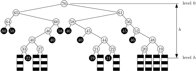
Next, the right child of is labelled and colored by following the same rules but with the block . We continue processing nodes in bfs fashion. A black or gray node in the tree is a leaf and is not processed any further. A white node with label is processed in the same way we processed the key , but with its two blocks and . We continue recursively constructing the tree until all the leaves are black or gray. See Figure 6 for an example of a full history tree.
Notice that the full history tree is totally deterministic as it does not contain any random value. It is also clear that the full history tree contains at least one gray leaf and every internal (white) node in the tree has two children. Furthermore, since the insertion process is sequential, node values (key numbers) along any path down from the root must be decreasing (so the binary tree has the heap property), because any non-gray child of any node represents the last key inserted in the block containing it at the insertion time of the parent. We will not use the heap property however.
Clearly, the full history tree permits one to deduce the load of the block that contains the root key at the time of its insertion: it is the length of the shortest path from the root to any gray node. Thus, if the block’s load is more than , then all gray nodes must be at distance more than from the root. This leads to the notion of a truncated history tree of height , that is, with levels of nodes. The top part of the full history tree that includes all nodes at the first levels is copied, and the remainder is truncated.
We are in particular interested in truncated history trees without gray nodes. Thus, by the property mentioned above, the length of the shortest path from the root to any gray node (and as noted above, there is at least one such node) would have to be at least , and therefore, the load of the block harboring the root’s key would have to be at least . More generally, if the load is at least for a positive integer , then all nodes at the bottom level of the truncated history tree that are not black nodes (and there is at least one such node) must be white nodes whose children represent keys that belong to blocks with load of at least at their insertion time. We redraw these node as boxes to denote the fact that they represent blocks of load at least , and we call them “block” nodes.
The Witness Tree
Let be a fixed integer to be picked later. For positive integers and , where , a witness tree is a truncated history tree of a key in the set , with levels of nodes (thus, of height ) and with two types of leaf nodes, black nodes and “block” nodes. This means that each internal node has two children, and the node labels belong to the set . Each black leaf has a label of an internal node that precedes it in bfs order. Block nodes are unlabelled nodes that represent blocks with load of at least . Block nodes must all be at the furthest level from the root, and there is at least one such node in a witness tree. Notice that every witness tree is deterministic. An example of a witness tree is shown in Figure 7.
Let denote the class of all witness trees of height that have white (internal) nodes, and black nodes (and thus block nodes). Notice that, by definition, the class could be empty, e.g., if , or . However, , which is due to the following. Without the labelling, there are at most different shape binary trees, because the shape is determined by the internal nodes, and hence, the number of trees is the Catalan number . Having fixed the shape, each of the leaves is of one of two types. Each black leaf can receive one of the white node labels. Each of the white nodes gets one of possible labels.
Note that, unlike the full history tree, not every key has a witness tree : the key must be placed into a block of load of at least just before the insertion time. We say that a witness tree occurs, if upon execution of algorithm WalkFirst, the random choices available for the keys represented by the witness tree are actually as indicated in the witness tree itself. Thus, a witness tree of height exists if and only if there is a key that is inserted into a block of load of at least before the insertion.
Before we embark on the proof of Theorem 10, we highlight three important facts whose proofs are provided in the appendix. First, we bound the probability that a valid witness tree occurs.
Lemma 4.
Let denote the event that the number of blocks in WalkFirst with load of at least , after termination, is at most , for some constant . For , let be the event that after the insertion of keys, none of the blocks is fully loaded. Then for any positive integers and , and a non-negative integer , we have
The next lemma asserts that the event in Lemma 4 is most likely to be true, for sufficiently large .
Lemma 5.
Let , , and be as defined in Theorem 10. Let be the number of blocks with load of at least upon termination of algorithm WalkFirst. If , then , for any constant .
Lemma 6 addresses a simple but crucial fact. If the height of a witness tree is , then the number of white nodes is at least two, (namely, the root and its left child); but what can we say about , the number of black nodes?
Lemma 6.
In any witness tree , if and , where , then the number of black nodes is , i.e., .
Proof of Theorem 10.
Recall that , for , is the event that after the insertion of keys (i.e., at time ), none of the blocks is fully loaded. Notice that , and the event is deterministically true. We shall show that . Let denote the event that the number of blocks with load of at least , after termination, is at most , for some constant to be decided later. Observe that
Lemma 5 reveals that , and hence, we only need to demonstrate that , for . We do that by using the witness tree argument. Let be some integers to be picked later such that . If after the insertion of keys, there is a block with load of at least , then a witness tree (with block nodes representing blocks with load of at least ) must have occurred. Recall that the number of white nodes in any witness tree is at least two. Using Lemmas 4 and 6, we see that
Note that we disallow , because any witness tree has at least one block node. We split the sum over , and . For , we have , and thus
provided that is so large that , (this insures that ). For , we bound trivially, assuming the same large condition:
In summary, we see that
We set , and , so that , because . With this choice, we have
where . Clearly, if we put , and , then we see that , and . Notice that and satisfy the technical condition , asymptotically.
Tradeoffs
We have seen that by using two linear probe sequences instead of just one, the maximum unsuccessful search time decreases exponentially from to . The average search time, however, could at worst double as shown in the simulation results. Most of the results presented in this article can be improved, by a constant factor though, by increasing the number of hashing choices per key. For example, Theorems 5 and 6 can be easily generalized for open addressing hashing schemes that use linear probe sequences. Similarly, all the two-way linear probing algorithms we design here can be generalized to -way linear probing schemes. The maximum unsuccessful search time will, then, be at most , where is a constant depending on . This means that the best worst-case performance is when where the minimum of is attained. The average search time, on the other hand, could triple.
The performance of these algorithms can be further improved by using Vöcking’s scheme LeftMC, explained in Section 2, with hashing choices. The maximum unsuccessful search time, in this case, is at most , for some constant depending on . This is minimized when , but we know that it can not get better than , because .
5 Simulation Results
We simulate all linear probing algorithms we discussed in this article with the fcfs replacement strategy: the classical linear probing algorithm ClassicLinear, the locally linear algorithm LocallyLinear, and the two-way linear probing algorithms ShortSeq, SmallCluster, WalkFirst, and DecideFirst. For each value of , and constant , we simulate each algorithm 1000 times divided into 10 iterations (experiments). Each iteration consists of 100 simulations of the same algorithm where we insert keys into a hash table with cells. In each simulation we compute the average and the maximum successful search and insert times. For each iteration (100 simulations), we compute the average of the average values and and the average of the maximum values computed during the 100 simulations for the successful search and insert times. The overall results are finally averaged over the 10 iterations and recorded in the next Tables. Similarly, the average maximum cluster size is computed for each algorithm as it can be used to bound the maximum unsuccessful search time, as mentioned earlier. Notice that in the case of the algorithms ClassicLinear and ShortSeq, the successful search time is the same as the insertion time.
Tables 1 and 2 contain the simulation results of the algorithms ClassicLinear, ShortSeq, and SmallCluster. With the exception of the average insertion time of SmallCluster Algorithm, which is slightly bigger than ClassicLinear Algorithm, it is evident that the average and the worst-case performances of SmallCluster and ShortSeq are better than ClassicLinear. Algorithm SmallCluster seems to have the best worst-case performance among the three algorithms. This is not a total surprise to us, because the algorithm considers more information (relative to the other two) before it makes its decision of where to insert the keys. It is also clear that there is a nonlinear increase, as a function of , in the difference between the performances of these algorithms. This may suggest that the worst-case performances of algorithms ShortSeq and SmallCluster are roughly of the order of .
| ClassicLinear | ShortSeq | SmallCluster | SmallCluster | ||||||
|---|---|---|---|---|---|---|---|---|---|
| Insert/Search Time | Insert/Search Time | Search Time | Insert Time | ||||||
| Avg | Max | Avg | Max | Avg | Max | Avg | Max | ||
| 0.4 | 1.33 | 5.75 | 1.28 | 4.57 | 1.28 | 4.69 | 1.50 | 9.96 | |
| 0.9 | 4.38 | 68.15 | 2.86 | 39.72 | 3.05 | 35.69 | 6.63 | 71.84 | |
| 0.4 | 1.33 | 10.66 | 1.28 | 7.35 | 1.29 | 7.49 | 1.52 | 14.29 | |
| 0.9 | 5.39 | 275.91 | 2.90 | 78.21 | 3.07 | 66.03 | 6.91 | 118.34 | |
| 0.4 | 1.33 | 16.90 | 1.28 | 10.30 | 1.29 | 10.14 | 1.52 | 18.05 | |
| 0.9 | 5.49 | 581.70 | 2.89 | 120.32 | 3.07 | 94.58 | 6.92 | 155.36 | |
| 0.4 | 1.33 | 23.64 | 1.28 | 13.24 | 1.29 | 13.03 | 1.52 | 21.41 | |
| 0.9 | 5.50 | 956.02 | 2.89 | 164.54 | 3.07 | 122.65 | 6.92 | 189.22 | |
| 0.4 | 1.33 | 26.94 | 1.28 | 14.94 | 1.29 | 14.44 | 1.52 | 23.33 | |
| 0.9 | 5.50 | 1157.34 | 2.89 | 188.02 | 3.07 | 136.62 | 6.93 | 205.91 | |
| ClassicLinear | ShortSeq | SmallCluster | |||||
|---|---|---|---|---|---|---|---|
| Avg | Max | Avg | Max | Avg | Max | ||
| 0.4 | 2.02 | 8.32 | 1.76 | 6.05 | 1.76 | 5.90 | |
| 0.9 | 15.10 | 87.63 | 12.27 | 50.19 | 12.26 | 43.84 | |
| 0.4 | 2.03 | 14.95 | 1.75 | 9.48 | 1.75 | 9.05 | |
| 0.9 | 15.17 | 337.22 | 12.35 | 106.24 | 12.34 | 78.75 | |
| 0.4 | 2.02 | 22.54 | 1.75 | 12.76 | 1.75 | 12.08 | |
| 0.9 | 15.16 | 678.12 | 12.36 | 155.26 | 12.36 | 107.18 | |
| 0.4 | 2.02 | 29.92 | 1.75 | 16.05 | 1.75 | 15.22 | |
| 0.9 | 15.17 | 1091.03 | 12.35 | 203.16 | 12.35 | 136.19 | |
| 0.4 | 2.02 | 33.81 | 1.75 | 17.74 | 1.75 | 16.65 | |
| 0.9 | 15.17 | 1309.04 | 12.35 | 226.44 | 12.35 | 150.23 | |
The simulation data of algorithms LocallyLinear, WalkFirst, and DecideFirst are presented in Tables 3, 4 and 5. These algorithms are simulated with blocks of size . The purpose of this is to show that, practically, the additive and the multiplicative constants appearing in the definitions of the block sizes stated in Theorems 8, 9 and 10 can be chosen to be small. The hash table is partitioned into equal-sized blocks, except possibly the last one. The average and the maximum values of the successful search time, inset time, and cluster size (averaged over 10 iterations each consisting of 100 simulations of the algorithms) are recorded in the tables below where the best performances are drawn in boldface.
Results show that LocallyLinear Algorithm has the best performance; whereas algorithm WalkFirst appears to perform better than DecideFirst. Indeed, the sizes of the cluster produced by algorithm WalkFirst appears to be very close to that of LocallyLinear Algorithm. This supports the conjecture that Theorem 10 is, in fact, true for any constant load factor , and the maximum unsuccessful search time of WalkFirst is at most , w.h.p. The average maximum cluster size of algorithm DecideFirst seems to be close to the other ones when is small; but it almost doubles when is large. This may suggest that the multiplicative constant in the maximum unsuccessful search time established in Theorem 9 could be improved.
| LocallyLinear | WalkFirst | DecideFirst | |||||
|---|---|---|---|---|---|---|---|
| Avg | Max | Avg | Max | Avg | Max | ||
| 0.4 | 1.73 | 4.73 | 1.78 | 5.32 | 1.75 | 5.26 | |
| 0.9 | 4.76 | 36.23 | 4.76 | 43.98 | 5.06 | 59.69 | |
| 0.4 | 1.74 | 6.25 | 1.80 | 7.86 | 1.78 | 7.88 | |
| 0.9 | 4.76 | 47.66 | 4.80 | 67.04 | 4.94 | 108.97 | |
| 0.4 | 1.76 | 7.93 | 1.80 | 9.84 | 1.78 | 10.08 | |
| 0.9 | 4.78 | 56.40 | 4.89 | 89.77 | 5.18 | 137.51 | |
| 0.4 | 1.76 | 8.42 | 1.81 | 12.08 | 1.79 | 12.39 | |
| 0.9 | 4.77 | 65.07 | 4.98 | 108.24 | 5.26 | 162.04 | |
| 0.4 | 1.76 | 9.18 | 1.81 | 12.88 | 1.79 | 13.37 | |
| 0.9 | 4.80 | 71.69 | 5.04 | 118.06 | 5.32 | 181.46 | |
| LocallyLinear | WalkFirst | DecideFirst | |||||
|---|---|---|---|---|---|---|---|
| Avg | Max | Avg | Max | Avg | Max | ||
| 0.4 | 1.14 | 2.78 | 2.52 | 6.05 | 1.15 | 3.30 | |
| 0.9 | 2.89 | 22.60 | 6.19 | 48.00 | 3.19 | 42.64 | |
| 0.4 | 1.14 | 3.38 | 2.53 | 8.48 | 1.17 | 5.19 | |
| 0.9 | 2.91 | 27.22 | 6.28 | 69.30 | 3.16 | 84.52 | |
| 0.4 | 1.15 | 4.08 | 2.53 | 10.40 | 1.17 | 6.56 | |
| 0.9 | 2.84 | 31.21 | 6.43 | 91.21 | 3.17 | 106.09 | |
| 0.4 | 1.15 | 4.64 | 2.54 | 12.58 | 1.18 | 8.16 | |
| 0.9 | 2.89 | 35.21 | 6.54 | 109.71 | 3.22 | 117.42 | |
| 0.4 | 1.15 | 4.99 | 2.54 | 13.41 | 1.18 | 8.83 | |
| 0.9 | 2.91 | 38.75 | 6.61 | 119.07 | 3.26 | 132.83 | |
| LocallyLinear | WalkFirst | DecideFirst | |||||
|---|---|---|---|---|---|---|---|
| Avg | Max | Avg | Max | Avg | Max | ||
| 0.4 | 1.57 | 4.34 | 1.65 | 4.70 | 1.63 | 4.81 | |
| 0.9 | 12.18 | 33.35 | 12.54 | 34.40 | 13.48 | 47.76 | |
| 0.4 | 1.62 | 6.06 | 1.68 | 6.32 | 1.68 | 6.82 | |
| 0.9 | 12.42 | 48.76 | 12.78 | 51.80 | 13.45 | 94.98 | |
| 0.4 | 1.62 | 7.14 | 1.68 | 7.31 | 1.68 | 8.92 | |
| 0.9 | 12.66 | 59.61 | 12.98 | 62.24 | 13.53 | 125.40 | |
| 0.4 | 1.65 | 8.25 | 1.71 | 8.50 | 1.71 | 10.76 | |
| 0.9 | 12.83 | 67.23 | 13.11 | 69.45 | 13.62 | 145.30 | |
| 0.4 | 1.62 | 8.90 | 1.71 | 8.95 | 1.71 | 11.46 | |
| 0.9 | 12.72 | 65.58 | 13.19 | 73.22 | 13.66 | 164.45 | |
Comparing the simulation data from all tables, one can see that the best average performance is achieved by the algorithms LocallyLinear and ShortSeq. Notice that ShortSeq Algorithm achieves the best average successful search time when . The best (average and maximum) insertion time is achieved by the algorithm LocallyLinear. On the other hand, algorithms WalkFirst and LocallyLinear are superior to the others in worst-case performance. It is worth noting that surprisingly, the worst-case successful search time of algorithm SmallCluster is very close to the one achieved by WalkFirst and better than that of DecideFirst, although, it appears that the difference becomes larger, as increases.
Appendix
For completeness, we prove the lemmas used in the proof of Theorem 10.
Lemma 4.
Let denote the event that the number of blocks in WalkFirst with load of at least , after termination, is at most , for some constant . For , let be the event that after the insertion of keys, none of the blocks is fully loaded. Then for any positive integers and , and a non-negative integer , we have
Proof.
Notice first that given , the probability that any fixed key in the set chooses a certain block is at most . Let be a fixed witness tree. We compute the probability that occurs given that is true, by looking at each node in bfs order. Suppose that we are at an internal node, say , in . We would like to find the conditional probability that a certain child of node is exactly as indicated in the witness tree, given that is true, and everything is revealed except those nodes that precede in the bfs order. This depends on the type of the child. If the child is white or black, the conditional probability is not more than . This is because each key refers to the unique block that contains it, and moreover, the initial hashing cells of all keys are independent. Multiplying just these conditional probabilities yields , as there are edges in the witness tree that have a white or black nodes as their lower endpoint. On the other hand, if the child is a block node, the conditional probability is at most . This is because a block node corresponds to a block with load of at least , and there are at most such blocks each of which is chosen with probability of at most . Since there are block nodes, the result follows plainly by multiplying all the conditional probabilities. ∎
To prove Lemma 5, we need to recall the following binomial tail inequality [69]: for , and any positive integers , and , for some , we have
where , which is decreasing on . Notice that , for any , because , for some .
Lemma 5.
Let , , and be as defined in Theorem 10. Let be the number of blocks with load of at least upon termination of algorithm WalkFirst. If , then , for any constant .
Proof.
Fix . Let denote the last block in the hash table, i.e., consists of the cells . Let be the load of after termination. Since the loads of the blocks are identically distributed, we have
Let be the set of the consecutively occupied cells, after termination, that occur between the first empty cell to the left of the block and the cell ; see Figure 8.
We say that a key is born in a set of cells if at least one of its two initial hashing cells belong to . For convenience, we write to denote the number of keys that are born in . Obviously, is . Since the cell adjacent to the left boundary of is empty, all the keys that are inserted in are actually born in . That is, if , then . So, by the binomial tail inequality given earlier, we see that
where the constant , because . Let
and notice that for large enough,
where , because . Clearly, by the same property of stated above, ; and hence, by the binomial tail inequality again, we conclude that for sufficiently large,
Thence, which implies by Markov’s inequality that
∎
Lemma 6.
In any witness tree , if and , where , then the number of black nodes is , i.e., .
Proof.
Note that any witness tree has at least one block node at distance from the root. If we have black nodes, the number of block nodes is at least . Since , then . If , then we have a contradiction. So, assume . But then ; that is, . ∎
References
- [1] M. Adler, P. Berenbrink, and K. Schroeder, “Analyzing an infinite parallel job allocation process,” in: Proceedings of the European Symposium on Algorithms, pp.417–428, 1998.
- [2] M. Adler, S. Chakrabarti, M. Mitzenmacher, and L. Rasmussen, “Parallel randomized load balancing,” in: Proceedings of the 27th Annual ACM Symposium on Theory of Computing (STOC), pp. 238–247, 1995.
- [3] D. Aldous, “Hashing with linear probing, under non-uniform probabilities,” Probab. Eng. Inform. Sci., vol. 2, pp. 1–14, 1988.
- [4] O. Aichholzer, F. Aurenhammer, and G. Rote, “Optimal graph orientation with storage applications”, SFB-Report F003-51, SFB ’Optimierung und Kontrolle’, TU-Graz, Austria, 1995.
- [5] Y. Azar, A. Z. Broder, A. R. Karlin and E. Upfal, “Balanced allocations,” SIAM Journal on Computing, vol. 29:1, pp. 180–200, 2000.
- [6] G. de Balbine, Computational Analysis of the Random Components Induced by Binary Equivalence Relations, Ph.D. Thesis, Calif. Inst. of Tech., 1969.
- [7] P. Berenbrink, A. Czumaj, T. Friedetzky, and N. D. Vvedenskaya, “Infinite parallel job allocations,” in: Proceedings of the 11th Annual ACM Symposium on Parallel Algorithms and Architectures (SPAA), pp. 99–108, 2000.
- [8] P. Berenbrink, A. Czumaj, A. Steger, and B. Vöcking, “Balanced allocations: the heavily loaded case,” SIAM Journal on Computing, vol. 35 (6), pp. 1350–1385, 2006.
- [9] B. Bollobás, A. Z. Broder, and I. Simon, “The cost distribution of clustering in random probing,” Journal of the ACM, vol. 37 (2), pp. 224–237, 1990.
- [10] R. P. Brent, “Reducing the retrieval time of scatter storage techniques,” Communications of the ACM, vol. 16 (2), pp. 105–109, 1973.
- [11] A. Z. Broder and A. Karlin, “Multilevel adaptive hashing,” in: Proceedings of the 1st Annual ACM-SIAM Symposium on Discrete Algorithms (SODA), ACM Press, pp. 43–53, 2000.
- [12] A. Broder and M. Mitzenmacher, “Using multiple hash functions to improve IP lookups,” in: Proceedings of 20th Annual Joint Conference of the IEEE Computer and Communications Societies (INFOCOM 2001), pp. 1454–1463, 2001. Full version available as Technical Report TR–03–00, Department of Computer Science, Harvard University, Cambridge, MA, 2000.
- [13] P. Celis, “Robin Hood hashing,” Ph.D. thesis, Computer Science Department, University of Waterloo, 1986. Available also as Technical Report CS-86-14.
- [14] P. Celis, P. Larson, and J. I. Munro, “Robin Hood hashing (preliminary report),” in: Proceedings of the 26th Annual IEEE Symposium on Foundations of Computer Science (FOCS), pp. 281–288, 1985.
- [15] P. Chassaing and G. Louchard, “Phase transition for parking blocks, Brownian excursion and coalescence,” Random Structures Algorithms, vol. 21 (1), pp. 76–119, 2002.
- [16] R. Cole, A. Frieze, B. M. Maggs, M. Mitzenmacher, A. W. Richa, R. K. Sitaraman, and E. Upfal, “On balls and bins with deletions,” in: Proceedings of the 2nd International Workshop on Randomization and Approximation Techniques in Computer Science, LNCS 1518, Springer-Verlag, pp. 145–158, 1998.
- [17] R. Cole, B. M. Maggs, F. Meyer auf der Heide, M. Mitzenmacher, A. W. Richa, K. Schroeder, R. K. Sitaraman, and B. Voecking, “Randomized protocols for low-congestion circuit routing in multistage interconnection networks,” in: Proceedings of the 29th Annual ACM Symposium on the Theory of Computing (STOC), pp. 378–388, 1998.
- [18] A. Czumaj and V. Stemann, “Randomized Allocation Processes,” Random Structures and Algorithms, Vol. 18 (4), pp. 297–331, 2001.
- [19] K. Dalal, L. Devroye. E. Malalla, and E. McLeish, “Two-way chaining with reassignment,” SIAM Journal on Computing, Vol. 35 (2), pp 327–340, 2005.
- [20] L. Devroye, “The expected length of the longest probe sequence for bucket searching when the distribution is not uniform,” Journal of Algorithms, vol. 6, pp. 1–9, 1985.
- [21] L. Devroye and P. Morin, “Cuckoo hashing: further analysis,” Information Processing Letters, vol. 86, pp. 215-219, 2003.
- [22] L. Devroye, P. Morin, and A. Viola, “On worst-case Robin Hood hashing,” SIAM Journal on Computing, vol. 33, pp. 923–936, 2004.
- [23] M. Dietzfelbinger and F. Meyer auf der Heide, “A new universal class of hash functions and dynamic hashing in real time,” in: Proceedings of the 17th International Colloquium on Automata, Languages and Programming, LNCS 443, Springer-Verlag, pp. 6–19, 1990.
- [24] M. Dietzfelbinger and F. Meyer auf der Heide, “High performance universal hashing, with applications to shared memory simulations,” in: Data Structures and Efficient Algorithms, LNCS 594, Springer-Verlag, pp. 250–269, 1992.
- [25] M. Dietzfelbinger and C. Weidling, “Balanced allocation and dictionaries with tightly packed constant size bins,” Theoretical Computer Science, vol. 380, pp. 47–68, 2007.
- [26] M. Dietzfelbinger and P. Wolfel, “Almost random graphs with simple hash functions,” in: Proceedings of the 35th Annual ACM Symposium on Theory of Computing (STOC), pp. 629–638, 2003.
- [27] M. Dietzfelbinger, J. Gil, Y. Matias, and N. Pippenger, “Polynomial hash functions are reliable (extended abstract),” in: Proceedings of the 19th International Colloquium on Automata, Languages and Programming, LNCS 623, Springer-Verlag, pp. 235–246, 1992.
- [28] M. Dietzfelbinger, A. Karlin, K. Mehlhorn, F. Meyer auf der Heide, H. Rohnert, and R. Tarjan, “Dynamic perfect hashing: upper and lower bounds,” SIAM Journal on Computing, vol. 23 (4), pp. 738–761, 1994.
- [29] D. Dubhashi, and D. Ranjan, “Balls and bins: a study in negative dependence,” Random Structures and Algorithms, vol. 13 (2), pp. 99–124, 1998.
- [30] D. L. Eager, E. D. Lazowska, and J. Zahorjan, “Adaptive load sharing in homogeneous distributed systems,” IEEE Transactions on Software Engineering, vol. 12, pp. 662–675, 1986.
- [31] J. D. Esary, F. Proschan, and D. W. Walkup, “Association of random variables, with applications,” Annals of Mathematical Statistics, vol. 38, pp. 1466–1474, 1967.
- [32] P. Flajolet, P. V. Poblete, and A. Viola, “On the analysis of linear probing hashing,” Algorithmica, vol. 22, pp. 490–515, 1998.
- [33] D. Fotakis, R. Pagh, P. Sanders, and P. G. Spirakis, “Space efficient hash tables with worst case constant access time,” in: Proceedings of the 20th Symposium on Theoretical Aspects of Computer Science, LNCS 2607, Springer-Verlag, pp. 271–282, 2003.
- [34] N. Fountoulakis and K. Panagiotou, “Sharp Load Thresholds for Cuckoo Hashing,” Random Structures and Algorithms, vol. 41 (3), pp. 306–333, 2012.
- [35] N. Fountoulakis, K. Panagiotou, and A. Steger, “On the Insertion Time of Cuckoo Hashing,” SIAM Journal on Computing, vol. 42, pp. 2156–2181, 2013.
- [36] M. Fredman, J. Komlós, and E. Szemerédi, “Storing a sparse table with worst case access time,” Journal of the ACM, vol. 31, pp. 538–544, 1984.
- [37] A. M. Frieze and P. Melsted, “Maximum Matchings in Random Bipartite Graphs and the Space Utilization of Cuckoo Hash Tables,” Random Structures and Algorithms, vol. 41 (3), pp. 334–364, 2012.
- [38] A. M. Frieze, P. Melsted, and M. Mitzenmacher, “An analysis of random-walk cuckoo hashing,” SIAM Journal on Computing, vol. 40 (2), pp. 291–308, 2011.
- [39] G. H. Gonnet, “Open addressing hashing with unequal-probability keys,” Journal of Computer and System Sciences, vol. 20, pp. 354–367, 1980.
- [40] G. H. Gonnet, “Expected length of the longest probe sequence in hash code searching,” Journal of the ACM, vol. 28, pp. 289–304, 1981.
- [41] G. H. Gonnet and R. Baeza-Yates, Handbook of Algorithms and Data Structures, Addison-Wesley, Workingham, 1991.
- [42] G. H. Gonnet and J. I. Munro, ‘’Efficient ordering of hash tables,” SIAM Journal on Computing, Vol. 8 (3), pp. 463–478, 1979.
- [43] L. J. Guibas, “The analysis of hashing techniques that exhibit -ary clustering,” Journal of the ACM, vol. 25 (4), pp. 544–555, 1978.
- [44] S. Janson, “Asymptotic distribution for the cost of linear probing hashing,” Random Structures and Algorithms, vol. 19 (3–4), pp. 438–471, 2001.
- [45] S. Janson, “Individual displacements for linear probing hashing with different insertion policies,” Technical Report No. 35, Department of Mathematics, Uppsala University, 2003.
- [46] S. Janson and A. Viola, “A unified approach to linear probing hashing with buckets,” Algorithmica, vol. 75 (4), pp.724–781, 2016.
- [47] K. Joag-Dev and F. Proschan, “Negative association of random variables, with applications”, Annals of Statistics, vol. 11 (4), pp. 286–295, 1983.
- [48] N. L. Johnson and S. Kotz, Urn Models and Their Application: An Approach to Modern Discrete Probability Theory, John Wiley, New York, 1977.
- [49] R. Karp, M. Luby, and F. Meyer auf der Heide, “Efficient PRAM simulation on a distributed memory machine,” Algorithmica, vol. 16, pp. 245–281, 1996.
- [50] D. E. Knuth, “Notes on “open” addressing,” Unpublished notes, 1963. Available at http://www.wits.ac.za/helmut/first.ps.
- [51] D. E. Knuth, The Art of Computer Programming, Vol. 3: Sorting and Searching, Addison-Wesley, Reading, Mass., 1973.
- [52] D. E. Knuth, “Linear probing and graphs, average-case analysis for algorithms,” Algorithmica, vol. 22 (4), pp. 561–568, 1998.
- [53] V. F. Kolchin, B. A. Sevast’yanov, and V. P. Chistyakov, Random Allocations, V. H. Winston & Sons, Washington, D.C., 1978.
- [54] A. G. Konheim and B. Weiss, “An occupancy discipline and applications,” SIAM Journal on Applied Mathematics, vol. 14, pp. 1266–1274, 1966.
- [55] P. Larson, “Analysis of uniform hashing,” Journal of the ACM, vol. 30 (4), pp. 805–819, 1983.
- [56] E. Lehman and R. Panigrahy, “3.5-Way Cuckoo Hashing for the Price of 2-and-a-Bit,” in: Proceedings of the 17th Annual European Symposium, pp. 671–681, 2009.
- [57] G. S. Lueker and M. Molodowitch, “More analysis of double hashing,” Combinatorica, vol. 13 (1), pp. 83–96, 1993.
- [58] J. A. T. Madison, “Fast lookup in hash tables with direct rehashing,” The Computer Journal, vol. 23 (2), pp. 188–189, 1980.
- [59] E. Malalla, Two-way Hashing with Separate Chaining and Linear Probing, Ph.D. thesis, School of Computer Science, McGill University, 2004.
- [60] E. G. Mallach, “Scatter storage techniques: a uniform viewpoint and a method for reducing retrieval times,” The Computer Journal, vol. 20 (2), pp. 137–140, 1977.
- [61] H. Mendelson and U. Yechiali, “A new approach to the analysis of linear probing schemes,” Journal of the ACM, vol. 27 (3), pp. 474–483, 1980.
- [62] F. Meyer auf der Heide, C. Scheideler, and V. Stemann, “Exploiting storage redundancy to speed up randomized shared memory simulations,” in: Theoretical Computer Science, Series A, Vol. 162 (2), pp. 245–281, 1996.
- [63] M. D. Mitzenmacher, The Power of Two Choices in Randomized Load Balancing, Ph.D. thesis, Computer Science Department, University of California at Berkeley, 1996.
- [64] M. Mitzenmacher, “Studying balanced allocations with differential equations,” Combinatorics, Probability, and Computing, vol. 8, pp. 473–482, 1999.
- [65] M. Mitzenmacher and B. Vöcking, “The asymptotics of Selecting the shortest of two, improved,” in: Proceedings of the 37th Annual Allerton Conference on Communication, Control, and Computing, pp. 326–327, 1998.
- [66] M. D. Mitzenmacher, A. Richa, and R. Sitaraman, “The power of two random choices: A survey of the techniques and results,” in: Handbook of Randomized Computing, (P. Pardalos, S. Rajasekaran, and J. Rolim, eds.), pp. 255–305, 2000.
- [67] R. Morris, “Scatter storage techniques,” Communications of the ACM, vol. 11 (1), pp. 38–44, 1968.
- [68] J. I. Munro and P. Celis, “Techniques for collision resolution in hash tables with open addressing,” in: Proceedings of 1986 Fall Joint Computer Conference, pp. 601–610, 1999.
- [69] M. Okamoto, “Some inequalities relating to the partial sum of binomial probabilities,” Annals of Mathematical Statistics, vol. 10, pp. 29–35, 1958.
- [70] A. Östlin and R. Pagh, “Uniform hashing in constant time and linear space,” in: Proceedings of the 35th Annual ACM Symposium on Theory of Computing (STOC), pp. 622–628, 2003.
- [71] R. Pagh, “Hash and displace: Efficient evaluation of minimal perfect hash functions,” in: Proceedings of the 6th International Workshop on Algorithms and Data Structures, LNCS 1663, Springer-Verlag, pp. 49–54, 1999.
- [72] R. Pagh, “On the cell probe complexity of membership and perfect hashing,” in: Proceedings of 33rd Annual ACM Symposium on Theory of Computing (STOC), pp. 425–432, 2001.
- [73] A. Pagh, R. Pagh, and M. Ružić, “Linear probing with 5-wise independence,” SIAM Review, vol. 53 (3), pp. 547–558, 2011.
- [74] R. Pagh and F. F. Rodler, “Cuckoo hashing,” in: Proceedings of the European Symposium on Algorithms, LNCS 2161, Springer-Verlag, pp. 121–133, 2001.
- [75] W. W. Peterson, “Addressing for random-access storage,” IBM Journal of Research and Development, vol. 1 (2), pp. 130–146, 1957.
- [76] G. C. Pflug and H. W. Kessler, “Linear probing with a nonuniform address distribution,” Journal of the ACM, vol. 34 (2), pp. 397–410, 1987.
- [77] B. Pittel, “Linear probing: The probable largest search time grows logarithmically with the number of records,” Journal of Algorithms, vol. 8, pp. 236–249, 1987.
- [78] P. V. Poblete and J. I. Munro, “Last-Come-First-Served hashing,” Journal of Algorithms, vol. 10, pp. 228–248, 1989.
- [79] P. V. Poblete, A. Viola, and J. I. Munro, “Analyzing the LCFS linear probing hashing algorithm with the help of Maple,” Maple Technical Newletter vol. 4 (1), pp. 8–13, 1997.
- [80] M. Raab and A. Steger, ““Balls and bins” – a simple and tight analysis,” in: Proceedings of the 2nd Workshop on Randomization and Approximation Techniques in Computer Science, LNCS 1518, Springer-Verlag, pp. 159–170, 1998.
- [81] S. Richter, V. Alvarez, and J. Dittrich, “A seven-dimensional analysis of hashing methods and its implications on query processing,” in: Porceedings of the VLDB Endowment, vol. 9 (3), pp. 96–107, 2015.
- [82] R. L. Rivest, “Optimal arrangement of keys in a hash table,” Journal of the ACM, vol. 25 (2), pp. 200–209, 1978.
- [83] T. Schickinger and A. Steger, “Simplified witness tree arguments,” in: Proceedings of the 27th Annual Conference on Current Trends in Theory and Practice of Informatics, LNCS 1963, Springer-Verlag, pp. 71–87, 2000.
- [84] J. P. Schmidt and A. Siegel, “Double hashing is computable and randomizable with universal hash functions,” submitted. A full version is available as Technical Report TR1995-686, Computer Science Department, New York University, 1995.
- [85] A. Siegel, “On universal classes of extremely random constant time hash functions and their time-space tradeoff,” Technical Report TR1995-684, Computer Science Department, New York University, 1995. A previous version appeared under the title “On universal classes of fast high performance hash functions, their time-space tradeoff and their applications,” in: Proceedings of the 30th Annual IEEE Symposium on Foundations of Computer Science (FOCS), pp. 20–25, 1989.
- [86] A. Siegel and J. P. Schmidt, “Closed hashing is computable and optimally randomizable with universal hash functions,” submitted. A full version is available as Technical Report TR1995-687, Computer Science Department, New York University, 1995.
- [87] V. Stemann, “Parallel balanced allocations”, in: Proceedings of the 8th Annual ACM Symposium on Parallel Algorithms and Architectures (SPAA), pp. 261–269, 1996.
- [88] M. Thorup and Y. Zhang, “Tabulation-based 5-independent hashing with applications to linear probing and second moment estimation,” SIAM Journal on Computing, vol. 41 (2), pp. 293–331, 2012.
- [89] J. D. Ullman, “A note on the efficiency of hashing functions,” Journal of the ACM, vol. 19 (3), pp. 569–575, 1972.
- [90] A. Viola, “Exact distributions of individual displacements in linear probing hashing,” ACM Transactions on Algorithms, vol. 1 (2), pp. 214–242, 2005.
- [91] A. Viola and P. V. Poblete, “The analysis of linear probing hashing with buckets”, Algorithmica, vol. 21, pp. 37–71, 1998.
- [92] J. S. Vitter and P. Flajolet, “Average-case analysis of algorithms and data structures,” in: Handbook of Theoretical Computer Science, Volume A: Algorithms and Complexity, ed. J. van Leeuwen, pp. 431–524, MIT Press, Amsterdam, 1990.
- [93] B. Vöcking, “How asymmetry helps load balancing,” Journal of the ACM, vol. 50 (4), pp. 568–589, 2003.
- [94] B. Vöcking, “Symmetric vs. asymmetric multiple-choice algorithms,” in: Proceedings of the 2nd ARACNE Workshop, Aarhus, pp. 7–15, 2001.
- [95] S. Walzer, “Load thresholds for cuckoo hashing with overlapping blocks,” in: Proceedings of the 45th International Colloquium on Automata, Languages, and Programming, pp. 102:1–102:10, 2018.
- [96] J. Wu and L. Kobbelt, “Fast mesh decimation by multiple-choice techniques,” in: Proceedings of Vision, Modeling, and Visualization, pp. 241–248, 2002.
- [97] A. C. Yao, “Uniform hashing is optimal,” Journal of the ACM, vol. 32 (3), pp. 687–693, 1985.