Morley Type Virtual Element Method for Von Kármán Equations

Abstract

This paper analyses the nonconforming Morley type virtual element method to approximate a regular solution to the von Kármán equations  that describes bending of very thin elastic plates. Local existence and uniqueness of a discrete solution to the non-linear problem is discussed. A priori error estimate in the energy norm is established under minimal regularity assumptions on the exact solution. Error estimates in piecewise $H^{1}$ and $L^{2}$ norm are also derived. A working procedure to find an approximation for the discrete solution using Newtons method is discussed. Numerical results that justify theoretical estimates are presented.

1 Introduction

The von Kármán equations  [24, 30, 9] model the bending of very thin elastic plates through a system of fourth-order semi-linear elliptic equations defined by: for a given load $f\in L^{2}(\Omega)$, seek the vertical displacement $u$ and the Airy stress function $v$ such that

$$\Delta^{2}u=[u,v]+f\text{ and }\Delta^{2}v=-\frac{1}{2}[u,u]\text{ in }\Omega,$$ (1.1a)

$$u=\frac{\partial u}{\partial n}=v=\frac{\partial v}{\partial n}=0\text{ on }\partial\Omega,$$ (1.1b)

with the von Kármán bracket $\displaystyle[\eta,\chi]:=\eta_{xx}\chi_{yy}+\eta_{yy}\chi_{xx}-2\eta_{xy}\chi_{xy}$ and $n$ is the unit outward normal to the boundary $\partial\Omega$ of the polygonal domain $\Omega\subseteq\mathbb{R}^{2}$.

The major challenges of the problem in its numerical approximation are the non-linearity and the higher order nature of the equations. The results regarding the existence of solutions, regularity and bifurcation phenomena of the von Kármán equations  in (1.1) are presented in [24, 30, 8, 7, 9, 10] and the references therein. It is well-known [10] that the solutions of the von Kármán equations  belong to $H^{2}_{0}(\Omega)\cap H^{2+\alpha}(\Omega)$, where $\alpha\in(\frac{1}{2},1]$, referred to as the index of elliptic regularity, is determined by the interior angles of $\Omega$. Note that when $\Omega$ is convex, $\alpha=1$.

The numerical methods to approximate the regular solutions of von Kármán equations  has been studied using conforming finite element methods (FEMs) in [17, 32], nonconforming Morley FEM in [33, 20], mixed FEMs in [35, 21, 37], discontinuous Galerkin methods, $C^{0}$ interior penalty methods in [11, 19], and hybrid FEMs in [36]. More recently, a conforming virtual element method is analysed in [31].

The Virtual Element Method (VEM) [5], which is a generalization of the FEM, has got more and more attention in recent years, because it can deal with the polygonal meshes and avoid an explicit construction of the discrete shape function, [25, 6, 14]. The polytopal meshes can be very useful for a wide range of reasons, including meshing of the domain (such as cracks) and data features, automatic use of hanging nodes, adaptivity. A conforming VEM for plate bending problems is introduced in [18]. A $C^{1}$ virtual element for the Cahn-Hilliard equations and the vibration problem of Kirchhoff plates is developed in [3], . This has been extended to the von Kármán equations  to approximate the regular solutions in [31]. In [38], a $C^{0}$ noncoforming VEM for plate bending problems is constructed for any order of accuracy. This nonconforming method is modified to fully nonconforming Morley type VEM in [39, 4]. Note that both these papers deal with the same degrees of freedom whereas use different definition on the local virtual space. Recently, the Morley type VEM is analysed for the Navier-Stokes equations in stream function vorticity formulation in [1].

The aim of this paper is to extend and analyze the nonconforming Morley type VEM presented in [39] to approximate a regular solution to the von Kármán equations. Since the discrete space is not a subspace of $H^{2}_{0}(\Omega)$, the convergence analysis offers a lot of challenges and novelty for this semilinear problem with trilinear nonlinearity. The trilinear form in [1] for the Navier-Stokes equation in stream-function form vanishes whenever the second and third variables are equal, and satisfies the anti-symmetric property with respect to the second and third variables, and this aids the wellposedness of the discrete formulation and error analysis. However, the trilinear form for von Kármán equations  does not satisfy the properties stated above and hence leads to interesting challenges in the analysis. A discrete version of Sobolev embedding is employed for establishing the well-posedness of the discrete linearized problem or equivalently a discrete inf-sup condition. This discrete inf-sup condition allows the proof of local existence and uniqueness of a discrete solution to the non-linear problem with a Banach fixed point theorem. Optimal order error estimate in $H^{2}$ and $H^{1}$ norms are established using minimal regularity assumption of the exact solution. The discrete non-linear problem can be solved using the Newton’s method by choosing an appropriate initial guess such that there exists a closed sphere in which the approximate solution is unique and the Newton’s iterates converge quadratically to the discrete solution.

The remaining parts are organised as follows. Section 2 discusses the weak formulation of the von Kármán equations  and the linearised problem. Section 3 deals with the Morley type VEM for the von Kármán equations. Some auxiliary results required for the convergence analysis and the wellposedness for the discrete linearised problem are established in Section 4 and is followed by the existence and local uniqueness of the discrete solution using fixed point of a non-linear operator. A priori error control in $H^{2}$ and $H^{1}$ norms, and convergence of the Newtons method are derived in Section 5. Section 6 provides the results of computational experiments that validate the theoretical estimates.

Throughout the paper, standard notations on Lebesgue and Sobolev spaces and their norms are employed. The standard semi-norm and norm on $H^{s}(\Omega)$ (resp. $W^{s,p}(\Omega)$) for $s>0$ and $1\leq p\leq\infty$ are denoted by $|\cdot|_{s}$ and $\|\cdot\|_{s}$ (resp. $|\cdot|_{s,p}$ and $\|\cdot\|_{s,p}$ ). The norm in $H^{-s}(\Omega)$ is denoted by $\|\cdot\|_{-s}$. The standard $L^{2}$ inner product and norm are denoted by $(\cdot,\cdot)$ and $\|\cdot\|.$ The notation ${\bm{H}}^{s}(\Omega)$ (resp. ${\bm{L}}^{p}(\Omega)$) is used to denote the product space $H^{s}(\Omega)\times H^{s}(\Omega)$ (resp. $L^{p}(\Omega)\times L^{p}(\Omega)$). For all $\Phi=(\varphi_{1},\varphi_{2})\in{\bm{H}}^{s}(\Omega)\;(\text{ resp. }{\bm{L}}^{2}(\Omega))$, the product space is equipped with the norm $\|{\Phi}\|_{s}:=(\|\varphi_{1}\|_{s}^{2}+\|\varphi_{2}\|_{s}^{2})^{1/2}\;(\text{ resp. }\|{\Phi}\|:=(\|\varphi_{1}\|^{2}+\|\varphi_{2}\|^{2})^{1/2}).\;$ The notation $a\lesssim b$ (resp. $a\gtrsim b$) means there exists a generic mesh independent constant $C$ such that $a\leq Cb$ (resp. $a\geq Cb$).

2 Weak formulation

This section deals with the continuous weak formulation and its linearisation of the von Kármán equations.

For all $\eta,\chi,\varphi\in V:=H^{2}_{0}(\Omega)$, the weak formulation associated with (1.1) seeks $u,v\in\>V$ such that, for all $(\varphi_{1},\varphi_{2})\in{\mathbf{V}}=:V\times V$,

$$a(u,\varphi_{1})+b(u,v,\varphi_{1})+b(v,u,\varphi_{1})=f(\varphi_{1})$$ (2.1a)

$$a(v,\varphi_{2})-b(u,u,\varphi_{2})=0,$$ (2.1b)

with, for all $\eta,\chi,\varphi\in V$,

$$a(\eta,\chi):=\int_{\Omega}D^{2}\eta:D^{2}\chi{\rm\,dx},\quad f(\varphi):=\int_{\Omega}f\varphi{\rm\,dx}\mbox{ and }$$

$$b(\eta,\chi,\varphi):=-\frac{1}{2}\int_{\Omega}[\eta,\chi]\varphi{\rm\,dx}=\frac{1}{2}\int_{\Omega}{\rm cof}(D^{2}\eta)\nabla\chi\cdot\nabla\varphi{\rm\,dx},$$ (2.2)

where $D^{2}$ is the Hessian matrix, $:$ denotes the scalar product between the matrices and ${\rm cof}(D^{2}\eta)$ denotes the co-factor matrix of $D^{2}\eta$. It is known that (2.1a)-(2.1b) possesses at least one solution [30, 17, 24].

The combined vector form for (2.1a)-(2.1b) seeks $\Psi=(u,v)\in{\mathbf{V}}$ such that

$${A}(\Psi,\Phi)+B(\Psi,\Psi,\Phi)-{F}(\Phi)=0\quad\text{for all}\>\Phi\in{\mathbf{V}},$$ (2.3)

where, for all $\Xi=(\xi_{1},\xi_{2}),\Theta=(\theta_{1},\theta_{2})$, and $\Phi=(\varphi_{1},\varphi_{2})\in{\mathbf{V}}$,

$${A}(\Theta,\Phi):={}a(\theta_{1},\varphi_{1})+a(\theta_{2},\varphi_{2}),\;$$

$$B(\Xi,\Theta,\Phi):={}b(\xi_{1},\theta_{2},\varphi_{1})+b(\xi_{2},\theta_{1},\varphi_{1})-b(\xi_{1},\theta_{1},\varphi_{2}),\,\text{ and }\;$$

$${F}(\Phi):=(f(\varphi_{1}),0).$$

The trilinear form $b(\bullet,\bullet,\bullet)$ is symmetric in all the three variables and so is $B(\bullet,\bullet,\bullet)$. The boundedness and ellipticity properties stated below hold [24, 33]:

$${A}(\Theta,\Phi)\leq\|\Theta\|_{2}\>\|\Phi\|_{2},\>{A}(\Theta,\Theta)\geq\|\Theta\|_{2}^{2},\;\text{ and }\;B(\Xi,\Theta,\Phi)\lesssim\|\Xi\|_{2}\>\|\Theta\|_{2}\>\|\Phi\|_{2}.$$ (2.4)

Lemma 2.1 (a priori bounds).

[10, 34]For $f\in H^{-1}(\Omega)$, the solution $\Psi$ of (2.3) belongs to ${\mathbf{V}}\cap{\bm{H}}^{2+\alpha}(\Omega)$, $\alpha\in(1/2,1]$, and satisfies the $a~{}priori$ bounds $\|\Psi\|_{2}\lesssim\|f\|_{-1}$ and $\|\Psi\|_{2+\alpha}\lesssim\|f\|^{3}_{-1}+\|f\|_{-1}.$

Assume that the solution $\Psi=(u,v)$ is regular [17, 33]. That is, the linearised problem defined by: for given $G=(g_{1},g_{2})\in\bm{L}^{2}(\Omega)$, find $\Theta\in{\mathbf{V}}$ such that, for all $\Phi\in{\mathbf{V}}$,

$$\mathcal{A}(\Theta,\Phi):=A(\Theta,\Phi)+B(\Psi,\Theta,\Phi)+B(\Theta,\Psi,\Phi)=(G,\Phi)$$ (2.5)

is well-posed and satisfies the a priori bounds

$$\|\Theta\|_{2}\lesssim\|G\|\mbox{ and }\|\Theta\|_{2+\alpha}\lesssim\|G\|,$$ (2.6)

where $\alpha$ is the index of elliptic regularity. This is equivalent to an inf-sup condition

$$0<\beta:=\inf_{\begin{subarray}{c}\Theta\in{\mathbf{V}}\\ |\Theta|_{2}=1\end{subarray}}\sup_{\begin{subarray}{c}\Phi\in{\mathbf{V}}\\ |\Phi|_{2}=1\end{subarray}}\mathcal{A}(\Theta,\Phi).$$ (2.7)

It is well-known [30] that for sufficiently small $f$, the solution is unique and is a regular solution; but this paper aims at a local approximation of an arbitrary regular solution.

Let $\Psi$ be a regular solution to (3.16). Then the dual problem defined by: for $Q\in\bm{H}^{-1}(\Omega),$ find $\bm{\xi}\in{\mathbf{V}}$ such that

$$\mathcal{A}(\Phi,\bm{\xi})=(Q,\Phi)\quad\forall\,\Phi\in{\mathbf{V}}$$ (2.8)

is well-posed and satisfies the a priori bounds [33]:

$$\|\bm{\xi}\|_{2}\lesssim\|Q\|_{-1}\mbox{ and }\|\bm{\xi}\|_{2+\alpha}\lesssim\|Q\|_{-1}.$$ (2.9)

3 Morley type virtual element method

This section deals with the Morley type VEM proposed in [39] for (2.3). The Morley type virtual element is a nonconforming virtual element which has fewer degrees of freedom and not even $C^{0}$ continuous; it is a simplified version of the $C^{0}$ continuous nonconforming virtual element presented in [38].

Let $\mathcal{T}_{h}$ be a decomposition of $\Omega$ into non-overlapping simple polygons. Let ${\mathcal{E}}_{h}$ denotes the set of edges $e$ in $\mathcal{T}_{h}$ and $h_{K}$ denotes the diameter of the element $K$. Let $h_{\max}$ be the maximum of the diameters of all the elements of the mesh, i.e., $h_{\max}=\max_{K\in\mathcal{T}_{h}}h_{K}$. For any $K\in\mathcal{T}_{h}$, let $n_{K}$ denotes its unit outward normal vector along the boundary $\partial K$. The unit normal of an edge $e\in{\mathcal{E}}_{h}$ is denoted by $n_{e}$, whose orientation is chosen arbitrarily but fixed for internal edges and coinciding with the outward normal of $\Omega$ for boundary edges. Define the jump $\left[\hskip-3.5pt\left[\varphi\right]\hskip-3.5pt\right]_{e}:=\varphi|_{K_{+}}-\varphi|_{K_{-}}$ and the average $\langle\varphi\rangle_{e}:=\frac{1}{2}\left(\varphi|_{K_{+}}+\varphi|_{K_{-}}\right)$ across the interior edge $e$ of $\varphi\in H^{1}(\mathcal{T}_{h})$ of the adjacent triangles $K_{+}$ and $K_{-}$. Extend the definition of the jump and the average to an edge on boundary by $\left[\hskip-3.5pt\left[\varphi\right]\hskip-3.5pt\right]_{e}:=\varphi|_{e}$ and $\langle\varphi\rangle_{e}:=\varphi|_{e}$ for $e\in{\mathcal{E}}(\partial\Omega)$. For any vector function, the jump and the average are understood component-wise.

For a non-negative integer $m$ and $D\subseteq\mathbb{R}^{2}$, ${\mathcal{P}}_{m}(D)$ denotes the space of polynomials of degree atmost equal to $m$ on $D$ and

$${{\mathcal{P}}}_{m}(\mathcal{T}_{h}):=\{q\in L^{2}(\Omega):q|_{K}\in{{\mathcal{P}}}_{m}(K)\quad\forall\;K\in\mathcal{T}_{h}\}.$$

For $\Phi=(\varphi_{1},\varphi_{2})\in W^{m,p}(\mathcal{T}_{h})$, where $W^{m,p}(\mathcal{T}_{h})$ denotes the broken Sobolev space with respect to $\mathcal{T}_{h}$, $\|\Phi\|_{m,p,h}^{2}:=|\varphi_{1}|_{m,p,h}^{2}+|\varphi_{2}|_{m,p,h}^{2}$, and $|\varphi_{i}|_{m,p,h}=(\sum_{K\in\mathcal{T}}|\varphi_{i}|^{p}_{m,p,K})^{1/p}$, $i=1,2$; with $|\cdot|_{m,p,K}$ denoting the usual semi-norm in $W^{m,p}(K)$. When $p=2$, the corresponding norms are denoted by $\|\bullet\|_{m,h}$ and $|\bullet|_{m,h}$. The notation ${\bf X}$ is used to denote the product space $X\times X$.

Assume that there exists a positive real number $C_{\mathcal{T}}$ such that, for every $K\in\mathcal{T}_{h}$ [5]:

• $K\in\mathcal{T}_{h}$ is star-shaped with respect to every point of a ball of radius $C_{\mathcal{T}}h_{K}$,

• the ratio between the shortest edge and the diameter $h_{K}$ of $K$ is larger than $C_{\mathcal{T}}$.

From [22], we have that if the mesh $\mathcal{T}_{h}$ fulfilling the assumptions (A1) and (A2), then the mesh also satisfies the following property:

(P1): For each $K\in\mathcal{T}_{h}$, there exists a virtual triangulation $\mathcal{T}_{h}^{K}$ of $K$ such that $\mathcal{T}_{h}^{K}$ is uniformly shape regular and quasi-uniform. The corresponding mesh size $h_{T}$ of $\mathcal{T}_{h}^{K}$ is proportional to $h_{K}$. Every edge of $K$ is a side of a certain triangle in $\mathcal{T}_{h}^{K}$.

For every $K\in\mathcal{T}_{h}$, the local shape function space $\widetilde{V}_{h}(K)$ [38, 4] is defined by

$$\widetilde{V}_{h}(K):=\displaystyle\left\{\varphi\in H^{2}(K);\Delta^{2}\varphi=0,\varphi_{|e}\in{{\mathcal{P}}}_{2}(e),\Delta\varphi_{|e}\in{{\mathcal{P}}}_{0}(e),e\subseteq\partial K\right\}.$$ (3.1)

Obviously, ${{\mathcal{P}}}_{2}(K)\subseteq\widetilde{V}_{h}(K)$. The degrees of freedom on $\widetilde{V}_{h}(K)$ are

• The values of $\varphi(a_{i})$, $\forall$ vertex $a_{i}$,

• The moments $\displaystyle\frac{1}{h_{e}}\int_{e}\varphi{\rm\,ds}$, $\forall$ edge $e$,

• The moments $\displaystyle\int_{e}\frac{\partial\varphi}{\partial n_{e}}{\rm\,ds}$, $\forall$ edge $e$.

For each $K$ and any given $\varphi\in\widetilde{V}_{h}(K)$, define a projection operator $\Pi^{K}:\widetilde{V}_{h}(K)\to{{\mathcal{P}}}_{2}(K)\subseteq\widetilde{V}_{h}(K)$ as the solution to

$$a^{K}(\Pi^{K}\varphi,q) =a^{K}(\varphi,q)\quad\forall\;q\in P_{2}(K)$$ (3.2a)

$$\widehat{\Pi^{K}(\varphi)} =\widehat{\varphi}$$ (3.2b)

$$\int_{\partial K}\nabla\Pi^{K}\varphi{\rm\,ds} =\int_{\partial K}\nabla\varphi{\rm\,ds}$$ (3.2c)

such that $\Pi^{K}q=q$ for all $q\in{{\mathcal{P}}}_{2}(K)$ and $\Pi^{K}$ is computable from the above degrees of freedom. Here, $a^{K}(\bullet,\bullet)$ is the restriction of the continuous bilinear form $a(\bullet,\bullet)$ on the element $K$ and

$$\widehat{\varphi}=\frac{1}{n}\sum_{i=1}^{n}\varphi(a_{i}).$$ (3.3)

This $C^{0}$-nonconforming virtual element is modified to fully nonconforming virtual element in [39] such that the dimension of the shape function space and the degrees of freedom are reduced. Define the local shape function space $V_{h}(K)$ on a polygon $K$ by

$$V_{h}(K):=\left\{\varphi\in\widetilde{V}_{h}(K):\int_{e}\Pi^{K}\varphi{\rm\,ds}=\int_{e}\varphi{\rm\,ds}\;\forall e\subseteq\partial K\right\}.$$ (3.4)

Note that $\widetilde{V}_{h}(K)\subseteq V_{h}(K)$ and since $\Pi^{K}q=q$ for all $q\in{{\mathcal{P}}}_{2}(K)$, ${{\mathcal{P}}}_{2}(K)\subseteq V_{h}(K)$. The degrees of freedom on ${V}_{h}(K)$ are

• The values of $\varphi(a_{i})$, $\forall$ vertex $a_{i}$,

• The moments $\displaystyle\int_{e}\frac{\partial\varphi}{\partial n_{e}}{\rm\,ds}$, $\forall$ edge $e$.

Comparing with the degrees of freedom associated with $\widetilde{V}_{h}(K)$, the zero-order moments of $\varphi$ on edges are removed in the above degrees of freedom. Another fully nonconforming virtual element is presented in [4] with the same degrees of freedom as above, but with a different local virtual space.

Remark 3.1.

The special case of $V_{h}(K)$ with $K$ as a triangle together with 6 degrees of freedom leads to $V_{h}(K)={{\mathcal{P}}}_{2}(K)$. This shows that, for the (lowest-order) triangular case, the simplified nonconforming virtual element coincides with the Morley nonconforming finite element [23] with the same degrees of freedom. Hence, the simplified nonconforming virtual element can be viewed as the extension of the Morley element to polygonal meshes.

For every decomposition $\mathcal{T}_{h}$ of $\Omega$ into simple polygons $K$, define the global space $V_{h}$ by

$$V_{h}:=\Big{\{} \varphi_{h}\in L^{2}(\Omega);\,\varphi_{h|K}\in V_{h}(K)\,\forall\;K\in\mathcal{T}_{h},\varphi_{h}\text{ is continuous at the internal vertices}$$ (3.5)

$$\text{ and vanishes at the boundary vertices, }\int_{e}\left[\hskip-3.5pt\left[\frac{\partial\varphi_{h}}{\partial n_{e}}\right]\hskip-3.5pt\right]{\rm\,ds}=0\;\forall\;e\in{\mathcal{E}}_{h}\Big{\}}.$$ (3.6)

The global degrees of freedom on ${V}_{h}$ are

• The values of $\varphi_{h}(a_{i})$, $\forall$ internal vertex $a_{i}$,

• The moments $\displaystyle\int_{e}\frac{\partial\varphi_{h}}{\partial n_{e}}{\rm\,ds}$, $\forall$ internal edge $e$.

The space $V_{h}$ is not a subspace of $H^{2}_{0}(\Omega)$ and not even $C^{0}$ continuous over $\Omega$; hence the simplified virtual element is fully nonconforming. Moreover, $\dim(V_{h})=N_{V}+N_{E},$ where $N_{V}$ is the number of internal vertices of $\mathcal{T}_{h}$ and $N_{E}$ is the number of internal edges, see [39] for more details.

For each element $K\in\mathcal{T}_{h}$, let $\chi_{i}$ denote the operator associated with the $i$th degree of freedom, $i=1,\cdots,N^{K}$. The construction of $V_{h}$ shows that for every smooth enough function $\varphi$ there exists a unique element, usually known as the interpolant of $\varphi$ restricted to $K$, $\varphi_{I}^{K}\in V_{h}(K)$ such that

$$\chi_{i}(\varphi-\varphi_{I}^{K})=0,\quad i=1,\cdots,N^{K}.$$ (3.7)

Lemma 3.2 (Interpolation error).

[12, 39] For every $K\in\mathcal{T}_{h}$ and every $\varphi\in H^{s}(K)$ with $2\leq s\leq 3$, it holds that

$$\|\varphi-\varphi_{I}^{K}\|_{m,K}\lesssim h_{K}^{s-m}|\varphi|_{s,K},\quad m=0,1,2.$$

Lemma 3.3 (Polynomial error).

[12, 23, 39] For every $K\in\mathcal{T}_{h}$ and every $\varphi\in H^{s}(K)$ with $2\leq s\leq 3$, there exists a polynomial $\varphi_{\pi}^{K}\in{{\mathcal{P}}}_{2}(K)$ such that

$$\|\varphi-\varphi_{\pi}^{K}\|_{m,K}\lesssim h_{K}^{s-m}|\varphi|_{s,K},\quad m=0,1,2.$$

Also, $\|\varphi-\varphi_{\pi}^{K}\|_{1,4,K}\lesssim h_{K}^{s-3/2}|\varphi|_{s,K}.$

For each polygon $K$, define the discrete local bilinear form on $V_{h}(K)\times V_{h}(K)$ by

$$a_{h}^{K}(\varphi_{h},\psi_{h}):=a^{K}(\Pi^{K}\varphi_{h},\Pi^{K}\psi_{h})+S^{K}(\varphi_{h}-\Pi^{K}\varphi_{h},\psi_{h}-\Pi^{K}\psi_{h}),\,\forall\,\varphi_{h},\psi_{h}\in V_{h}(K),$$ (3.8)

where $\Pi^{K}$ is the projection operator defined in (3.2) and $S^{K}(\bullet,\bullet)$ is a symmetric and positive definite bilinear form satisfying

$$c_{0}a^{K}(\varphi_{h},\varphi_{h})\leq S^{K}(\varphi_{h},\varphi_{h})\leq c_{1}a^{K}(\varphi_{h},\varphi_{h})\quad\forall\;\varphi_{h}\in\ker(\Pi^{K})$$ (3.9)

for some positive constants $c_{0}$ and $c_{1}$ independent of $K$ and $h_{K}$. It is clear from (3.9) that $S^{K}$ must scale like $a^{K}(\bullet,\bullet)$ on the kernel of $\Pi^{K}$. As in [18], set

$$S^{K}(\varphi,\psi)=\sum_{i=1}^{N^{K}}\chi_{i}(\varphi)\chi_{i}(\psi)h_{i}^{-2},$$

where $h_{i}$ is the characteristic length attached to each degree of freedom $\chi_{i}$.

The standard arguments [5] reveals the consistency and stability properties of $a_{h}^{K}(\bullet,\bullet)$. That is,

$$a_{h}^{K}(p,\varphi_{h})=a^{K}(p,\varphi_{h})\quad\forall\,p\in{{\mathcal{P}}}_{2}(K),\,\forall\,\varphi_{h}\in V_{h}(K)$$ (3.10)

and there exists two positive constants $\alpha_{\ast}$ and $\alpha^{\ast}$ independent of $h$ and $K$ such that

$$\alpha_{\ast}a^{K}(\varphi_{h},\varphi_{h})\leq a_{h}^{K}(\varphi_{h},\varphi_{h})\leq\alpha^{\ast}a^{K}(\varphi_{h},\varphi_{h})\quad\forall\,\varphi_{h}\in V_{h}(K).$$ (3.11)

The global discrete bilinear form $a_{h}:V_{h}\times V_{h}\to\mathbb{R}$ is then defined by

$$a_{h}(\varphi_{h},\psi_{h}):=\sum_{K\in\mathcal{T}_{h}}a_{h}^{K}(\varphi_{h},\psi_{h})\quad\forall\;\varphi_{h},\psi_{h}\in V_{h}.$$ (3.12)

The construction of the discrete trilinear form associated with discrete weak formulation is as follows. Define, for all $\varphi_{h},\psi_{h},\theta_{h}\in V_{h}(K)$,

$$b_{h}^{K}(\varphi_{h},\psi_{h},\theta_{h})=\int_{K}{\rm cof}(D^{2}(\Pi^{K}\varphi_{h}))\nabla(\Pi^{K}\psi_{h})\cdot\nabla(\Pi^{K}\theta_{h}){\rm\,dx}.$$ (3.13)

Then the global discrete trilinear form $b_{h}:V_{h}\times V_{h}\times V_{h}\to\mathbb{R}$ is defined by

$$b_{h}(\varphi_{h},\psi_{h},\theta_{h}):=\sum_{K\in\mathcal{T}_{h}}b_{h}^{K}(\varphi_{h},\psi_{h},\theta_{h})\quad\forall\;\varphi_{h},\psi_{h},\theta_{h}\in V_{h}.$$ (3.14)

For constructing the linear form on the right-hand side, let $P_{0}^{K}(f)$ denote the $L^{2}$ projection of load $f$ onto ${{\mathcal{P}}}_{0}(K)$.Then the right hand side is defined by [39]

$$\langle f_{h},\varphi_{h}\rangle:=\sum_{K\in\mathcal{T}_{h}}(P_{0}^{K}(f),\widehat{\varphi_{h}})$$ (3.15)

with $\widehat{\varphi_{h}}$ from (3.3). The Morley type nonconforming virtual element discretisation associated with (2.3) seeks $\Psi_{h}:=(u_{h},v_{h})\in{\mathbf{V}}_{h}:=V_{h}\times V_{h}$ such that

$$A_{h}(\Psi_{h},\Phi_{h})+B_{h}(\Psi_{h},\Psi_{h},\Phi_{h})=F_{h}(\Phi_{h})\quad\forall\,\Phi_{h}\in{\mathbf{V}}_{h},$$ (3.16)

where for all $\Xi_{h}=(\xi_{1,h},\xi_{2,h}),\Theta_{h}=(\theta_{1,h},\theta_{2,h})$, and $\Phi=(\varphi_{1,h},\varphi_{2,h})\in{\mathbf{V}}_{h}$,

$${A}_{h}(\Theta_{h},\Phi_{h}):={}a_{h}(\theta_{1,h},\varphi_{1,h})+a_{h}(\theta_{2,h},\varphi_{2,h}),\;$$ (3.17a)

$$B_{h}(\Xi_{h},\Theta_{h},\Phi_{h}):={}b_{h}(\xi_{1,h},\theta_{2,h},\varphi_{1,h})+b_{h}(\xi_{2,h},\theta_{1,h},\varphi_{1,h})-b_{h}(\xi_{1,h},\theta_{1,h},\varphi_{2,h}),$$ (3.17b)

$$F_{h}(\Phi_{h})=(\langle f_{h},\varphi_{1,h}\rangle,0)$$ (3.17c)

with $a_{h}(\bullet,\bullet)$, $b_{h}(\bullet,\bullet,\bullet)$ and $\langle f_{h},\bullet\rangle$ from (3.12), (3.14), and (3.15) respectively.

For all $\varphi+\varphi_{h},\psi+\psi_{h},\theta+\theta_{h}\in V+V_{h}$, extend the definition of $b_{h}^{K}(\bullet,\bullet,\bullet)$ on $V_{h}(K)$ to $\widehat{b}_{h}^{K}(\bullet,\bullet,\bullet)$ on $V+V_{h}(K)$ as

$$\widehat{b}_{h}^{K}(\varphi+\varphi_{h},\psi+\psi_{h},\theta+\theta_{h})=\int_{K}{\rm cof}(D^{2}(\varphi+\Pi^{K}\varphi_{h}))\nabla(\psi+\Pi^{K}\psi_{h})\cdot\nabla(\theta+\Pi^{K}\theta_{h}){\rm\,dx}.$$ (3.18)

Then the global discrete trilinear form $\widehat{b}_{h}:(V+V_{h})\times(V+V_{h})\times(V+V_{h})\to\mathbb{R}$ is defined by

$$\widehat{b}_{h}(\varphi+\varphi_{h},\psi+\psi_{h},\theta+\theta_{h}):=\sum_{K\in\mathcal{T}_{h}}\widehat{b}_{h}^{K}(\varphi+\varphi_{h},\psi+\psi_{h},\theta+\theta_{h}).$$ (3.19)

For all $\Xi_{h}=(\xi_{1,h},\xi_{2,h}),\Theta_{h}=(\theta_{1,h},\theta_{2,h})$, and $\Phi=(\varphi_{1,h},\varphi_{2,h})\in{\mathbf{V}}+{\mathbf{V}}_{h}$,

$$\widehat{B}_{h}(\Xi_{h},\Theta_{h},\Phi_{h}):={}\widehat{b}_{h}(\xi_{1,h},\theta_{2,h},\varphi_{1,h})+\widehat{b}_{h}(\xi_{2,h},\theta_{1,h},\varphi_{1,h})-\widehat{b}_{h}(\xi_{1,h},\theta_{1,h},\varphi_{2,h}).$$ (3.20)

The Morley type nonconforming virtual element formulation corresponding to the continuous linearised problem (2.5) seeks $\Theta_{h}\in\text{\bf V}_{h}$ such that

$$\mathcal{A}_{h}(\Theta_{h},\Phi_{h}):=A_{h}(\Theta_{h},\Phi_{h})+\widehat{B}_{h}(\Psi,\Theta_{h},\Phi_{h})+\widehat{B}_{h}(\Theta_{h},\Psi,\Phi_{h})=G_{h}(\Phi_{h})\quad\forall\,\Phi_{h}\in\text{\bf V}_{h},$$ (3.21)

where $G_{h}(\Phi_{h})=(\langle g_{1,h},\varphi_{1,h}\rangle,\langle g_{2,h},\varphi_{2,h}\rangle)$ with $\langle\bullet,\bullet\rangle$ as in (3.15).

Define the broken semi-norm on $V_{h}$ by

$$|\varphi_{h}|_{m,h}:=\left(\sum_{K\in\mathcal{T}_{h}}|\varphi_{h}|_{m,K}^{2}\right)^{1/2},\quad m=1,2.$$ (3.22)

Then, the piecewise version of the energy norm in $H^{2}(\mathcal{T}_{h})\equiv\prod\limits_{K\in\mathcal{T}}H^{2}(K)$, $|\bullet|_{2,h}$, is a norm on $V_{h}$ [39, Lemma 5.1]. This, in particular, implies

$$\|\varphi_{h}\|^{2}+|\varphi_{h}|_{1,h}^{2}\lesssim|\varphi_{h}|_{2,h}^{2}.$$ (3.23)

4 Well-posedness, existence and uniqueness

This section presents some auxiliary results that are useful to establish the convergence analysis and is followed by the well-posedness of the discrete linearised problem in Section 4.1. Section 4.2 discusses the existence and local uniqueness of the discrete solution.

Lemma 4.1 (Boundedness and coercivity).

Any $\Phi_{h},\Theta_{h}\in{\mathbf{V}}_{h}$ satisfy

• $A_{h}(\Phi_{h},\Theta_{h})\lesssim|\Phi_{h}|_{2,h}|\Theta_{h}|_{2,h}$.

• $A_{h}(\Phi_{h},\Phi_{h})\gtrsim|\Phi_{h}|_{2,h}^{2}.$

• $F_{h}(\Phi_{h})\lesssim\|f\||\Phi_{h}|_{2,h}.$

Proof of (a). The symmetry of $a_{h}(\bullet,\bullet)$, (3.11), and the definition of $a^{K}(\bullet,\bullet)$ imply, for all $\varphi_{h},\theta_{h}\in V_{h}$,

$$a_{h}^{K}(\varphi_{h},\theta_{h})\leq(a_{h}^{K}(\varphi_{h},\varphi_{h}))^{1/2}(a_{h}^{K}(\theta_{h},\theta_{h}))^{1/2} \leq\alpha^{\ast}(a^{K}(\varphi_{h},\varphi_{h}))^{1/2}(a^{K}(\theta_{h},\theta_{h}))^{1/2}$$ (4.1)

$$=\alpha^{\ast}|\varphi_{h}|_{2,K}|\theta_{h}|_{2,K}.$$ (4.2)

The sum over all $K\in\mathcal{T}_{h}$, Hölder inequality, the definition of $|\bullet|_{2,h}$ in (3.22), and (3.17a) conclude the proof of $(a)$. ∎

Proof of (b). The estimate follows from the definition of $A_{h}(\bullet,\bullet)$ in (3.17a), the stability property (3.11), the definition of $a^{K}(\bullet,\bullet)$, and (3.22).∎

Proof of (c). The definition of $F_{h}(\bullet)$ in (3.17c), (3.15), Hölder inequality, $\|P_{0}^{K}f\|_{0,K}\lesssim\|f\|_{0,K}$, $\|\widehat{\varphi_{h}}-\varphi_{h}\|_{0,K}\lesssim h_{K}\|\varphi_{h}\|_{1,K}$ for $\varphi_{h}\in V_{h}$, and (3.23) concludes the proof of $(c)$. ∎

Since the discrete space $V_{h}$ is not a subspace of $V$, an enrichment operator ${E}_{h}$ which maps the nonconforming discrete space to the conforming space plays an important role in establishing the boundedness properties of the discrete trilinear form and hence to derive the local existence and uniqueness of the discrete solution, and a priori error estimates for the solution of von Kármán equations. For that, consider the local finite dimensional space [3, Section 2.2]:

$$\widehat{V}_{h}^{c}(K):=\Big{\{}\varphi_{h}\in H^{2}(K);\, \Delta^{2}\varphi_{h}\in{{\mathcal{P}}}_{2}(K),\,\varphi_{h}|_{\partial K}\in C^{0}(\partial K),\,\varphi_{h}|_{e}\in{{\mathcal{P}}}_{3}(e)\;\forall e\subseteq\partial K,$$ (4.3)

$$\nabla\varphi_{h|\partial K}\in C^{0}(\partial K)^{2},\,\frac{\partial\varphi_{h}}{\partial n_{e}}\big{|}_{e}\in{{\mathcal{P}}}_{1}(e)\;\forall e\subseteq\partial K\Big{\}}.$$ (4.4)

For $K\in\mathcal{T}_{h}$, the $H^{2}$ conforming local virtual finite element space $V_{h}^{c}(K)$ is then defined by

$$V_{h}^{c}(K):=\Big{\{}\varphi_{h}\in\widehat{V}_{h}^{c}(K);\, (\varphi_{h}-\Pi^{K,c}\varphi_{h},q)_{0,K}=0\,\forall\,q\in{{\mathcal{P}}}_{2}(K)\Big{\}},$$ (4.5)

where $\Pi^{K,c}:\widehat{V}_{h}^{c}(K)\to{{\mathcal{P}}}_{2}(K)\subseteq\widehat{V}_{h}^{c}(K)$ is the projection operator associated with the conforming virtual element, see [3, Section 2.2] for more details. The global $C^{1}$ virtual element space is

$$V_{h}^{c}:=\Big{\{}\varphi_{h}\in V;\,\varphi_{h}|_{K}\in{V}_{h}^{c}(K)\;\forall\;K\in\mathcal{T}_{h}\Big{\}}.$$ (4.6)

Let ${E}_{h}:V_{h}\to V_{h}^{c}$ be the enrichment operator. The properties of ${E}_{h}$ [1, Propostion 4.1], [29, Lemma 4.2] that are useful in the analysis are stated in the next lemma.

Lemma 4.2 (Enrichment operator).

For all ${\varphi}_{h}\in V_{h}$, ${E}_{h}{\varphi}_{h}\in V_{h}^{c}$ satisfies

$$\sum_{m=0}^{2}h_{K}^{m-2}|{\varphi}_{h}-{E}_{h}{\varphi}_{h}|_{m,K}\lesssim|{\varphi}_{h}|_{2,h}.$$

Lemma 4.3 (Discrete Sobolev embeddings).

[1, Theorem 4.1] For $2\leq q<\infty$, any ${\varphi}_{h}\in V_{h}$ satisfies $|{\varphi}_{h}|_{1,q,h}\lesssim|{\varphi}_{h}|_{2,h}.$

Recall the definition of $\Pi^{K}$ from (3.2). Define $\Pi^{h}$ in $L^{2}(\Omega)$ as, for all $v\in H^{2}(\mathcal{T}_{h})$,

$$(\Pi^{h}v)|_{K}:=\Pi^{K}v,\quad\forall\;K\in\mathcal{T}_{h}.$$ (4.7)

For $\varphi\in V_{h}$, a choice of $q=\Pi^{K}\varphi\in{{\mathcal{P}}}_{2}(K)$ in (3.2a) leads to $a^{K}(\Pi^{K}\varphi,\Pi^{K}\varphi)=a^{K}(\varphi,\Pi^{K}\varphi)$. The definition of $a^{K}(\bullet,\bullet)$ and Cauchy inequality imply $|\Pi^{K}\varphi|_{2,K}\leq|\varphi|_{2,K}.$ Consequently,

$$|\Pi^{h}\varphi|_{2,h}\leq|\varphi|_{2,h}.$$ (4.8)

Lemma 4.4 (Poincaré-Freidrich inequality and inverse estimates).

[15],[29, Lemma 3.2],[14, (2.8)] Any $\varphi\in H^{2}(K)$ satisfies

• $\displaystyle h_{K}^{-2}\|\varphi\|_{0,K}\lesssim|\varphi|_{2,K}+h_{K}^{-2}\left|\int_{\partial K}\varphi{\rm\,ds}\right|+h_{K}^{-1}\left|\int_{\partial K}\nabla\varphi{\rm\,ds}\right|$,

• $|\varphi|_{1,K}\lesssim h_{K}|\varphi|_{2,K}+h_{K}^{-1}\|\varphi\|_{0,K},$

• $\|\varphi\|_{0,\infty,K}\lesssim h_{K}^{-1}\|\varphi\|_{0,K}+|\varphi|_{1,K}+h_{K}|\varphi|_{2,K}.$

Lemma 4.5 (Projection error).

Any $K\in\mathcal{T}_{h}$ and $\varphi_{h}\in V_{h}$ satisfy

$$\|\varphi_{h}-\Pi^{K}\varphi_{h}\|_{0,K}+h_{K}|\varphi_{h}-\Pi^{K}\varphi_{h}|_{1,K}\lesssim h_{K}^{2}|\varphi_{h}-\Pi^{K}\varphi_{h}|_{2,K}.$$

Proof.

Since $\varphi_{h}\in V_{h}$, the choice $\varphi=\varphi_{h}-\Pi^{K}\varphi_{h}$ in Lemma 4.4.a, (3.4), and (3.2c) lead to $h_{K}^{-2}\|\varphi_{h}-\Pi^{K}\varphi_{h}\|_{0,K}\lesssim|\varphi_{h}-\Pi^{K}\varphi_{h}|_{2,K}$. A combination of this and Lemma 4.4.b shows $|\varphi_{h}-\Pi^{K}\varphi_{h}|_{1,K}\lesssim h_{K}|\varphi_{h}-\Pi^{K}\varphi_{h}|_{2,K}$. ∎

Recall the definition of $B_{h}(\bullet,\bullet,\bullet)$ and $\widehat{B}_{h}(\bullet,\bullet,\bullet)$ from (3.17b) and (3.20), and the index of elliptic regularity $\alpha\in(\frac{1}{2},1]$.

Lemma 4.6 (Bounds for $\widehat{B}_{h}(\bullet,\bullet,\bullet)$).

Any $\bm{\xi}\in{\mathbf{V}}\cap\bm{H}^{2+\alpha}(\Omega)$, $\Phi,\Theta\in{\mathbf{V}}$, and $\Phi_{h},\Theta_{h},\bm{\xi}_{h}\in{\mathbf{V}}_{h}$ satisfy

• $B_{h}(\Phi_{h},\Theta_{h},\bm{\xi}_{h})\lesssim|\Phi_{h}|_{2,h}|\Theta_{h}|_{2,h}|\bm{\xi}_{h}|_{2,h},$

• $\widehat{B}_{h}(\Theta+\Theta_{h},\Phi+\Phi_{h},\bm{\xi}+\bm{\xi}_{h})\lesssim|\Theta+\Pi^{h}\Theta_{h}|_{2,h}|\Phi+\Pi^{h}\Phi_{h}|_{1,4,h}|\bm{\xi}+\Pi^{h}\bm{\xi}_{h}|_{1,4,h},$

• $\widehat{B}_{h}(\bm{\xi},\Theta,\Phi+\Phi_{h})\lesssim\|\bm{\xi}\|_{2+\alpha}|\Theta|_{2}|\Phi+\Pi^{h}\Phi|_{1,h},$

• $\widehat{B}_{h}(\bm{\xi},\Theta_{h},\Phi+\Phi_{h})\lesssim\|\bm{\xi}\|_{2+\alpha}|\Theta_{h}|_{2,h}|\Phi+\Pi^{h}\Phi|_{1,h},$

• $\widehat{B}_{h}(\bm{\xi},\Phi+\Phi_{h},\Theta+\Theta_{h})\lesssim\|\bm{\xi}\|_{2+\alpha}|\Phi+\Pi^{h}\Phi_{h}|_{1,h}(|\Theta|_{2}+|\Theta_{h}|_{2,h}),$

• $\widehat{B}_{h}(\Theta+\Theta_{h},\bm{\xi},\Phi+\Phi_{h})\lesssim|\Theta+\Pi^{h}\Theta_{h}|_{2,h}\|\bm{\xi}\|_{2+\alpha}|\Phi+\Pi^{h}\Phi_{h}|_{1,h}.$

Proof of (a). For $\varphi_{h},\theta_{h},\xi_{h}\in V_{h}$, the definition of $b_{h}(\bullet,\bullet,\bullet)$ in (3.14) and a Hölder inequality show

$$b_{h}(\varphi_{h},\theta_{h},\xi_{h})\lesssim|\Pi^{h}\varphi_{h}|_{2,h}|\Pi^{h}\theta_{h}|_{1,4,h}|\Pi^{h}\xi_{h}|_{1,4,h}.$$

Lemma 4.3 for $q=4$ and (4.8) read $b_{h}(\varphi_{h},\theta_{h},\xi_{h})\lesssim|\varphi_{h}|_{2,h}|\theta_{h}|_{2,h}|\xi_{h}|_{2,h}$. This and the definition of $B_{h}(\bullet,\bullet,\bullet)$ in (3.17b) concludes the proof of $(a)$. ∎

Proof of (b). The result follows from the definition of $\widehat{b}_{h}(\bullet,\bullet,\bullet)$ in (3.19), a Hölder inequality (same as in $(a)$), and (3.20). ∎

Proof of (c). The definition of $\widehat{b}_{h}(\bullet,\bullet,\bullet)$ in (3.19) and a Hölder inequality lead to, for all $\xi\in V\cap H^{2+\alpha}(\Omega)$, $\varphi,\theta\in V$ and $\varphi_{h}\in V_{h}$,

$$\widehat{b}_{h}(\xi,\theta,\varphi+\varphi_{h})\lesssim|\xi|_{2,4}|\theta|_{1,4}|\varphi+\Pi^{h}\varphi_{h}|_{1,h}.$$ (4.9)

The Sobolev embeddings $H^{2+\alpha}(\Omega)\hookrightarrow W^{2,4}(\Omega)$ for $\alpha>1/2$ and $H^{2}(\Omega)\hookrightarrow W^{1,4}(\Omega)$ [16], and (3.20) concludes the proof of $(c)$. ∎

Proof of (d). A Hölder inequality reveals, for all $\xi\in V\cap H^{2+\alpha}(\Omega)$, $\varphi\in V$ and $\theta_{h},\varphi_{h}\in V_{h}$,

$$\widehat{b}_{h}(\xi,\theta_{h},\varphi+\varphi_{h})\lesssim|\xi|_{2,4}|\Pi^{h}\theta_{h}|_{1,4,h}|\varphi+\Pi^{h}\varphi_{h}|_{1,h}.$$ (4.10)

The Sobolev embedding $H^{2+\alpha}(\Omega)\hookrightarrow W^{2,4}(\Omega)$, Lemma 4.3, (4.8), and (3.20) proves the assertion of $(d)$. ∎

Proof of (e). The Hölder inequality, the Sobolev embeddings $H^{2+\alpha}(\Omega)\hookrightarrow W^{2,4}(\Omega)$, $H^{2}(\Omega)\hookrightarrow W^{1,4}(\Omega)$, and Lemma 4.3 provide

$$\widehat{b}_{h}(\xi,\varphi+\varphi_{h},\theta+\theta_{h}) \lesssim|\xi|_{2,4}|\varphi+\Pi^{h}\varphi_{h}|_{1,h}(|\theta|_{1,4}+|\Pi^{h}\theta_{h}|_{1,4,h})$$ (4.11)

$$\lesssim\|\xi\|_{2+\alpha}|\varphi+\Pi^{h}\varphi_{h}|_{1,h}(|\theta|_{2}+|\Pi^{h}\theta_{h}|_{2,h}).$$ (4.12)

This, (4.8), and (3.20) concludes the proof of $(e)$.∎

Proof of (f). The Hölder inequality and the Sobolev embedding $H^{2+\alpha}(\Omega)\hookrightarrow W^{1,\infty}(\Omega)$ [16] show

$$\widehat{b}_{h}(\theta+\theta_{h},\xi,\varphi+\varphi_{h}) \lesssim|\theta+\Pi^{h}\theta_{h}|_{2,h}|\xi|_{1,\infty}|\varphi+\Pi^{h}\varphi_{h}|_{1,h}$$

$$\lesssim|\theta+\Pi^{h}\theta_{h}|_{2,h}\|\xi\|_{2+\alpha}|\varphi+\Pi^{h}\varphi_{h}|_{1,h}.$$ (4.13)

A combination of (4) and (3.20) implies the assertion. ∎

Define, for all $\Theta_{h}=(\theta_{1,h},\theta_{2,h})$, and $\Phi=(\varphi_{1,h},\varphi_{2,h})\in{\mathbf{V}}+{\mathbf{V}}_{h}$,

$$A_{\rm{pw}}(\Theta_{h},\Phi_{h}):=\sum_{K\in\mathcal{T}_{h}}(a^{K}(\theta_{1,h},\varphi_{1,h})+a^{K}(\theta_{2,h},\varphi_{2,h})).$$ (4.14)

Define $\varphi_{\pi}^{h}\in{{\mathcal{P}}}_{2}(\mathcal{T}_{h})$ and $\varphi_{I}^{h}\in V_{h}$ by

$$\varphi_{\pi}^{h}|_{K}:=\varphi_{\pi}^{K}\quad\mbox{ and }\quad\varphi_{I}^{h}|_{K}:=\varphi_{I}^{K}$$

for all $K\in\mathcal{T}_{h}$, where $\varphi_{\pi}^{K}$ and $\varphi_{I}^{K}$ are as in Lemma 3.3 and 3.2.

Lemma 4.7 (Bounds for $A_{\rm{pw}}(\bullet,\bullet)$).

[2],[13, Lemmas 4.2, 4.3] Any $\bm{\xi}\in\bm{H}^{2+\alpha}(\Omega)$ for $\alpha\in(\frac{1}{2},1]$, $\Phi\in{\mathbf{V}}\cap\bm{H}^{2+\alpha}(\Omega)$, and $\Phi_{h}\in{\mathbf{V}}_{h}$ satisfy

• $A_{\rm{pw}}(\bm{\xi},E_{h}\Phi_{h}-\Phi_{h})\lesssim h_{\max}^{\alpha}\|\bm{\xi}\|_{2+\alpha}|\Phi_{h}|_{2,h},$

• $A_{\rm{pw}}(\bm{\xi},\Phi-\Phi_{I}^{h})\lesssim h_{\max}^{2\alpha}\|\bm{\xi}\|_{2+\alpha}\|\Phi\|_{2+\alpha}$, where $\Phi_{I}^{h}\in\text{\bf V}_{h}$ is the interpolant of $\Phi$.

Remark 4.8 (consequences of Lemma 3.2, 3.3, and 4.2).

The estimates in Lemma 3.2, 3.3, and 4.2 give rise some typical estimates utilised throughout the analysis in this paper. For $\varphi\in V\cap H^{2+\alpha}(\Omega)$, a triangle inequality with $\varphi$, Lemma 3.2, and Lemma 3.3 show

$$\|\varphi_{I}^{h}-\varphi_{\pi}^{h}\|_{2,h}\leq\|\varphi-\varphi_{I}^{h}\|_{2,h}+\|\varphi-\varphi_{\pi}^{h}\|_{2,h}\lesssim h_{\max}^{\alpha}\|\varphi\|_{2+\alpha}.$$ (4.15)

For $\varphi_{h}\in V_{h}$, triangle inequality with $\varphi_{h}$, Lemma 4.2, 4.5, and (4.8) provide

$$|E_{h}\varphi_{h}-\Pi^{h}\varphi_{h}|_{1,h}\leq|E_{h}\varphi_{h}-\varphi_{h}|_{1,h}+|\varphi_{h}-\Pi^{h}\varphi_{h}|_{1,h}\lesssim h_{\max}|\varphi_{h}|_{2,h}.$$ (4.16)

Analog arguments lead to $|E_{h}\varphi_{h}-\Pi^{h}\varphi_{h}|_{2,h}\lesssim|\varphi_{h}|_{2,h}$. Lemma 4.5, $\Pi^{h}\varphi_{\pi}^{h}=\varphi_{\pi}^{h}$, and (4.8) read

$$|\varphi_{I}^{h}-\Pi^{h}\varphi_{I}^{h}|_{1,h} \lesssim h_{\max}|\varphi_{I}^{h}-\Pi^{h}\varphi_{I}^{h}|_{2,h}\leq h_{\max}(|\varphi_{I}^{h}-\varphi_{\pi}^{h}|_{2,h}+|\Pi^{h}(\varphi_{\pi}^{h}-\varphi_{I}^{h})|_{2,h})$$ (4.17)

$$\lesssim h_{\max}|\varphi_{I}^{h}-\varphi_{\pi}^{h}|_{2,h}\lesssim h_{\max}^{1+\alpha}\|\varphi\|_{2+\alpha}$$ (4.18)

with (4.15) in the last step. This and Lemma 3.2 lead to

$$|\varphi-\Pi^{h}\varphi_{I}^{h}|_{1,h}\lesssim h_{\max}^{1+\alpha}\|\varphi\|_{2+\alpha}\;\mbox{ and }\;|\varphi-\Pi^{h}\varphi_{I}^{h}|_{2,h}\lesssim h_{\max}^{\alpha}\|\varphi\|_{2+\alpha}.$$ (4.19)

4.1 Well-posedness of the discrete problem

This section establishes the well-posedness of the discrete linearised problem (3.21).

Theorem 4.9 (Well-posedness of discrete linearised problem).

Let $\Psi\in{\mathbf{V}}\cap\bm{H}^{2+\alpha}(\Omega)$ be a regular solution to (3.16). Then for sufficiently small $h_{\max}$, the discrete linearised problem (3.21) is well-posed.

Proof.

Since ${\mathbf{V}}_{h}$ is finite dimensional and (3.21) is linear, establishing an a priori bound is sufficient to prove that (3.21) has a unique solution. The choice $\Phi_{h}=\Theta_{h}$ in (3.21), Lemma 4.1.b, 4.6.d and .f, and (4.8) lead to

$$G_{h}(\Theta_{h}) =\mathcal{A}_{h}(\Theta_{h},\Theta_{h})=A_{h}(\Theta_{h},\Theta_{h})+\widehat{B}_{h}(\Psi,\Theta_{h},\Theta_{h})+\widehat{B}_{h}(\Theta_{h},\Psi,\Theta_{h})$$

$$\gtrsim|\Theta_{h}|_{2,h}^{2}-\|\Psi\|_{2+\alpha}|\Theta_{h}|_{2,h}|\Pi^{h}\Theta_{h}|_{1,h}.$$ (4.20)

The arguments in the proof of Lemma 4.1.c show $G_{h}(\Theta_{h})\lesssim\|G\||\Theta_{h}|_{2,h}$. This with the above displayed inequality results in

$$|\Theta_{h}|_{2,h}\lesssim\|\Psi\|_{2+\alpha}|\Pi^{h}\Theta_{h}|_{1,h}+\|G\|.$$ (4.21)

The triangle inequality and (4.16) provide

$$|\Pi^{h}\Theta_{h}|_{1,h}\leq|\Pi^{h}\Theta_{h}-E_{h}\Theta_{h}|_{1,h}+|E_{h}\Theta_{h}|_{1}\lesssim h_{\max}|\Theta_{h}|_{2,h}+|E_{h}\Theta_{h}|_{1}.$$ (4.22)

To estimate $|E_{h}\Theta_{h}|_{1},$ choose $Q=-\Delta E_{h}\Theta_{h}$ and $\Phi=E_{h}\Theta_{h}$ in the dual problem (2.8). The definition of $\mathcal{A}(\bullet,\bullet)$ in (2.5) and (3.21) for $\Phi_{h}=\bm{\xi}_{I}^{h}$ read

$$|E_{h}\Theta_{h}|_{1}^{2} =A(E_{h}\Theta_{h},\bm{\xi})+B(\Psi,E_{h}\Theta_{h},\bm{\xi})+B(E_{h}\Theta_{h},\Psi,\bm{\xi})$$ (4.23)

$$=A_{\rm{pw}}(E_{h}\Theta_{h},\bm{\xi})+\widehat{B}_{h}(\Psi,E_{h}\Theta_{h},\bm{\xi}-\bm{\xi}_{I}^{h})+\widehat{B}_{h}(E_{h}\Theta_{h},\Psi,\bm{\xi}-\bm{\xi}_{I}^{h})$$

$$\quad+\widehat{B}_{h}(\Psi,E_{h}\Theta_{h},\bm{\xi}_{I}^{h})+\widehat{B}_{h}(E_{h}\Theta_{h},\Psi,\bm{\xi}_{I}^{h})-A_{h}(\Theta_{h},\bm{\xi}_{I}^{h})$$

$$\quad-\widehat{B}_{h}(\Psi,\Theta_{h},\bm{\xi}_{I}^{h})-\widehat{B}_{h}(\Theta_{h},\Psi,\bm{\xi}_{I}^{h})+G_{h}(\bm{\xi}_{I}^{h}).$$ (4.24)

Since $\bm{\xi}_{\pi}^{h}\in{{\mathcal{P}}}_{2}(\mathcal{T}_{h})$, the consistency property in (3.10) shows $A_{h}(\Theta_{h},\bm{\xi}_{\pi}^{h})=A_{\rm{pw}}(\Theta_{h},\bm{\xi}_{\pi}^{h}).$ This and elementary algebra reveal

$$|E_{h}\Theta_{h}|_{1,2,h}^{2} =A_{\rm{pw}}(E_{h}\Theta_{h}-\Theta_{h},\bm{\xi})+A_{\rm{pw}}(\Theta_{h},\bm{\xi}-\bm{\xi}_{\pi}^{h})+A_{h}(\Theta_{h},\bm{\xi}_{\pi}^{h}-\bm{\xi}_{I}^{h})$$

$$\quad+\widehat{B}_{h}(\Psi,E_{h}\Theta_{h},\bm{\xi}-\bm{\xi}_{I}^{h})+\widehat{B}_{h}(E_{h}\Theta_{h},\Psi,\bm{\xi}-\bm{\xi}_{I}^{h})$$

$$\quad+\widehat{B}_{h}(\Psi,E_{h}\Theta_{h}-\Theta_{h},\bm{\xi}_{I}^{h})+\widehat{B}_{h}(E_{h}\Theta_{h}-\Theta_{h},\Psi,\bm{\xi}_{I}^{h}-\bm{\xi})$$

$$\quad+\widehat{B}_{h}(E_{h}\Theta_{h}-\Theta_{h},\Psi,\bm{\xi})+G_{h}(\bm{\xi}_{I}^{h}):=T_{1}+\cdots+T_{9}.$$ (4.25)

Lemma 4.7 leads to $T_{1}\lesssim h_{\max}^{\alpha}\|\bm{\xi}\|_{2+\alpha}|\Theta_{h}|_{2,h}$. The Cauchy inequality and Lemma 3.3 show $T_{2}\lesssim h_{\max}^{\alpha}\|\bm{\xi}\|_{2+\alpha}|\Theta_{h}|_{2,h}$. Lemma 4.1.a, and (4.15) provide $T_{3}\lesssim h_{\max}^{\alpha}\|\bm{\xi}\|_{2+\alpha}|\Theta_{h}|_{2,h}$. Lemma 4.6.c, triangle inequality with $\Theta_{h}$, Lemma 4.2 and (4.19) read $T_{4}\lesssim h_{\max}^{1+\alpha}\|\bm{\xi}\|_{2+\alpha}|\Theta_{h}|_{2,h}$. Lemma 4.6.f shows $T_{5}\lesssim|E_{h}\Theta_{h}|_{2,h}\|\Psi\|_{2+\alpha}|\bm{\xi}-\Pi^{h}\bm{\xi}_{I}^{h}|_{1,h}$. Lemma 4.2 and (4.19) provide $T_{5}\lesssim h_{\max}^{1+\alpha}\|\bm{\xi}\|_{2+\alpha}|\Theta_{h}|_{2,h}$. Lemma 4.6.e, (4.16), and Lemma 3.2 reveal $T_{6}\lesssim h_{\max}\|\bm{\xi}\|_{2+\alpha}|\Theta_{h}|_{2,h}$. Lemma 4.6.f, Remark 4.8, and (4.19) lead to $T_{7}\lesssim h_{\max}^{1+\alpha}\|\bm{\xi}\|_{2+\alpha}|\Theta_{h}|_{2,h}$.

Since $\Psi,\bm{\xi}\in\text{\bf V}\cap\bm{H}^{2+\alpha}(\Omega)$, the Sobolev embedding $H^{2+\alpha}(\Omega)\hookrightarrow W^{2,4}(\Omega)$ shows

$$|\nabla\Psi\cdot\nabla\bm{\xi}|_{1}\leq|\nabla\Psi|_{1,4}|\nabla\bm{\xi}|_{1,4}\lesssim\|\Psi\|_{2+\alpha}\|\bm{\xi}\|_{2+\alpha}.$$

Hence, $\nabla\Psi\cdot\nabla\bm{\xi}\in H^{1}(\Omega)$ and $T_{8}\lesssim\sum_{K\in\mathcal{T}_{h}}|D^{2}(E_{h}\Theta_{h}-\Pi^{h}\Theta_{h})|_{-1,K}|\nabla\Psi\cdot\nabla\bm{\xi}|_{1,K}$. The definition of the dual norm and integration by parts lead to $|D^{2}(E_{h}\Theta_{h}-\Pi^{h}\Theta_{h})|_{-1,K}\lesssim|E_{h}\Theta_{h}-\Pi^{h}\Theta_{h}|_{1,K}$. The combination of the above estimates and Hölder inequality provides $T_{8}\lesssim|E_{h}\Theta_{h}-\Pi^{h}\Theta_{h}|_{1,h}\|\Psi\|_{2+\alpha}\|\bm{\xi}\|_{2+\alpha}$. This and (4.16) imply $T_{8}\lesssim h_{\max}\|\bm{\xi}\|_{2+\alpha}|\Theta_{h}|_{2,h}$. The same arguments in the proof of Lemma 4.1.c provides $T_{9}\lesssim\|G\||\bm{\xi}_{I}^{h}|_{2,h}\lesssim\|G\|\|\bm{\xi}\|_{2+\alpha}$ with Lemma 3.2 in the last step. A substitution of the estimates $T_{1},\cdots,T_{9}$ in (4.25) reads

$$|E_{h}\Theta_{h}|_{1}^{2}\lesssim(h_{\max}^{\alpha}|\Theta_{h}|_{2,h}+\|G\|)\|\bm{\xi}\|_{2+\alpha}.$$

Since $\|Q\|_{-1}=|E_{h}\Theta_{h}|_{1,2,h}$, the above displayed inequality and (2.9) imply

$$|E_{h}\Theta_{h}|_{1}\lesssim h_{\max}^{\alpha}|\Theta_{h}|_{2,h}+\|G\|.$$

The combination of the above displayed inequality, (4.22), and (4.21) results in

$$|\Theta_{h}|_{2,h}\leq C_{1}h_{\max}^{\alpha}|\Theta_{h}|_{2,h}+C\|G\|.$$

For a choice of $h_{\max}\leq h_{1}=\left(\frac{1}{2C_{1}}\right)^{\frac{1}{\alpha}}$, $|\Theta_{h}|_{2,h}\lesssim\|G\|$ and this implies the assertion. ∎

Remark 4.10.

Let $\Psi$ be a regular solution to (3.21). Then for a sufficiently small $h_{\max}$, the discrete linearised dual problem: given $Q\in\bm{L}^{2}(\Omega)$, find $\bm{\xi}_{h}\in{\mathbf{V}}_{h}$ such that

$$\mathcal{A}_{h}(\Phi_{h},\bm{\xi}_{h})=Q_{h}(\Phi_{h}),\forall\,\Phi_{h}\in\text{\bf V}_{h}$$

is well-posed, where $\mathcal{A}_{h}(\bullet,\bullet)$ is defined as in (3.21). The proof is similar to Theorem 4.9 and hence is skipped.

Since the discrete linearised problem and the dual problem are well-posed, $\mathcal{A}_{h}:{\mathbf{V}}_{h}\times{\mathbf{V}}_{h}\to\mathbb{R}$ defined by

$$\mathcal{A}_{h}(\Theta_{h},\Phi_{h}):=A_{h}(\Theta_{h},\Phi_{h})+\widehat{B}_{h}(\Psi,\Theta_{h},\Phi_{h})+\widehat{B}_{h}(\Theta_{h},\Psi,\Phi_{h})$$ (4.26)

satisifies discrete inf-sup condition on ${\mathbf{V}}_{h}\times{\mathbf{V}}_{h}$ [17, 33], that is, there exists a constant $\widehat{\beta}>0$ such that

$$\sup_{|\Theta_{h}|_{2,h}=1}\mathcal{A}_{h}(\Theta_{h},\Phi_{h})\geq\widehat{\beta}|\Phi_{h}|_{2,h}\mbox{ and }\sup_{|\Phi_{h}|_{2,h}=1}\mathcal{A}_{h}(\Theta_{h},\Phi_{h})\geq\widehat{\beta}|\Theta_{h}|_{2,h}.$$ (4.27)

Define the perturbed bilinear form by, for all $\Theta_{h},\Phi_{h}\in{\mathbf{V}}_{h}$,

$$\widehat{\mathcal{A}}_{h}(\Theta_{h},\Phi_{h}):=A_{h}(\Theta_{h},\Phi_{h})+B_{h}(\Psi_{I}^{h},\Theta_{h},\Phi_{h})+B_{h}(\Theta_{h},\Psi_{I}^{h},\Phi_{h}),$$ (4.28)

where $\Psi_{I}^{h}$ is the interpolant of $\Psi$.

Lemma 4.11.

Let $\Psi$ be a regular solution to (2.3). Then for a sufficiently small $h_{\max}$, the perturbed bilinear form $\widehat{\mathcal{A}}_{h}(\bullet,\bullet)$ in (4.28) satisfies discrete inf-sup condition on ${\mathbf{V}}_{h}\times{\mathbf{V}}_{h}$.

Proof.

Elementary algebra and (4.27) show

$$\sup_{|\Theta_{h}|_{2,h}=1}\widehat{\mathcal{A}}_{h} (\Theta_{h},\Phi_{h})=\sup_{|\Theta_{h}|_{2,h}=1}(A_{h}(\Theta_{h},\Phi_{h})+B_{h}(\Psi_{I}^{h},\Theta_{h},\Phi_{h})+B_{h}(\Theta_{h},\Psi_{I}^{h},\Phi_{h}))$$ (4.29)

$$\geq\sup_{|\Theta_{h}|_{2,h}=1}\mathcal{A}_{h}(\Theta_{h},\Phi_{h})-\sup_{|\Theta_{h}|_{2,h}=1}(\widehat{B}_{h}({\Psi}-\Psi_{I}^{h},\Theta_{h},\Phi_{h})+\widehat{B}_{h}(\Theta_{h},{\Psi}-\Psi_{I}^{h},\Phi_{h}))$$ (4.30)

$$\geq\widehat{\beta}|\Phi_{h}|_{2,h}-\sup_{|\Theta_{h}|_{2,h}=1}(\widehat{B}_{h}({\Psi}-\Psi_{I}^{h},\Theta_{h},\Phi_{h})+\widehat{B}_{h}(\Theta_{h},{\Psi}-\Psi_{I}^{h},\Phi_{h})).$$ (4.31)

Lemma 4.6.b, 4.3, and (4.8) imply $\widehat{B}_{h}({\Psi}-\Psi_{I}^{h},\Theta_{h},\Phi_{h})\lesssim|{\Psi}-\Pi^{h}\Psi_{I}^{h}|_{2,h}|\Phi_{h}|_{2,h}$. This and (4.19) provide $\widehat{B}_{h}({\Psi}-\Psi_{I}^{h},\Theta_{h},\Phi_{h})\leq C_{b}^{1}h_{\max}^{\alpha}\|\Psi\|_{2+\alpha}|\Phi_{h}|_{2,h}$. Lemma 4.6.b, 4.3, and (4.8) imply $\widehat{B}_{h}(\Theta_{h},{\Psi}-\Psi_{I}^{h},\Phi_{h})\lesssim|{\Psi}-\Pi^{h}\Psi_{I}^{h}|_{1,4,h}|\Phi_{h}|_{2,h}$. The relation $\Pi^{h}\Psi_{\pi}^{h}=\Psi_{\pi}^{h}$, inverse estimate for $\Pi^{h}({\Psi_{\pi}^{h}}-\Psi_{I}^{h})\in{{\mathcal{P}}}_{2}(\mathcal{T}_{h})$[12], and Lemma 3.3 show

$$|{\Psi}-\Pi^{h}\Psi_{I}^{h}|_{1,4,h} \leq|{\Psi}-\Psi_{\pi}^{h}|_{1,4,h}+|\Pi^{h}{(\Psi_{\pi}^{h}}-\Psi_{I}^{h})|_{1,4,h}$$

$$\lesssim h_{\max}^{\alpha+1/2}\|\Psi\|_{2+\alpha}+h_{\max}^{-1/2}|\Pi^{h}({\Psi_{\pi}^{h}}-\Psi_{I}^{h})|_{1,h}$$

$$\lesssim h_{\max}^{\alpha+1/2}\|\Psi\|_{2+\alpha}+h_{\max}^{-1/2}(|{\Psi_{\pi}^{h}}-\Psi_{I}^{h}|_{1,h}+|\Psi_{I}^{h}-\Pi^{h}\Psi_{I}^{h}|_{1,h})$$

$$\lesssim h_{\max}^{\alpha+1/2}\|\Psi\|_{2+\alpha}+h_{\max}^{-1/2}|\Psi_{I}^{h}-\Pi^{h}\Psi_{I}^{h}|_{1,h}$$ (4.32)

with Lemma 3.3 and 3.2 in the last step. This and (4.18) reveal

$$|{\Psi}-\Pi^{h}\Psi_{I}^{h}|_{1,4,h}\leq h_{\max}^{\alpha+1/2}\|\Psi\|_{2+\alpha}.$$ (4.33)

Consequently, $\widehat{B}_{h}(\Theta_{h},{\Psi}-\Psi_{I}^{h},\Phi_{h})\leq C_{b}^{2}h_{\max}^{\alpha}\|\Psi\|_{2+\alpha}|\Phi_{h}|_{2,h}$. Let $C_{b}:=\max\{C_{b}^{1},C_{b}^{2}\}$. Then, (4.31) shows

$$\sup_{|\Theta_{h}|_{2,h}=1}\widehat{\mathcal{A}}_{h} (\Theta_{h},\Phi_{h})\geq\widehat{\beta}|\Phi_{h}|_{2,h}-2C_{b}h_{\max}^{\alpha}\|\Psi\|_{2+\alpha}|\Phi_{h}|_{2,h}.$$ (4.34)

A choice of $\displaystyle h_{\max}\leq h_{2}=\left(\frac{\widehat{\beta}}{4C_{b}\|\Psi\|_{2+\alpha}}\right)^{1/\alpha}$ provides

$$\sup_{|\Theta_{h}|_{2,h}=1}\widehat{\mathcal{A}}_{h}(\Theta_{h},\Phi_{h})\geq({\widehat{\beta}}/{2})|\Phi_{h}|_{2,h}.$$

The analog arguments leads to $\displaystyle\sup_{|\Phi_{h}|_{2,h}=1}\widehat{\mathcal{A}}_{h}(\Phi_{h},\Theta_{h})\geq({\widehat{\beta}}/{2})|\Theta_{h}|_{2,h}.$ ∎

4.2 Existence and uniqueness

This section establishes the existence and uniqueness of the discrete solution and is an application of Brouwer’s fixed point theorem.

Theorem 4.12 (Existence and uniqueness of a discrete solution).

Let $\Psi$ be a regular solution to (2.3). For a sufficiently small choice of $h_{\max}$, there exists a unique solution $\Psi_{h}$ to the discrete (3.16) that satisfies $|\Psi_{h}-\Psi_{I}^{h}|_{2,h}\leq R(h_{\max})$ for some positive constant $R(h_{\max})$ depending on $h_{\max}$.

Proof.

Consider the non-linear mapping $T_{h}:\text{\bf V}_{h}\to\text{\bf V}_{h}$ defined by, for all $\Phi_{h}\in\text{\bf V}_{h}$,

$$\widehat{\mathcal{A}}_{h}(T_{h}(\Theta_{h}),\Phi_{h})=F_{h}(\Phi_{h})+B_{h}(\Psi_{I}^{h},\Theta_{h},\Phi_{h})+B_{h}(\Theta_{h},\Psi_{I}^{h},\Phi_{h})-B_{h}(\Theta_{h},\Theta_{h},\Phi_{h}).$$ (4.35)

Lemma 4.11 shows that the operator $T_{h}$ is well defined and continuous. It is easy to check that the any discrete solution $\Psi_{h}$ to (3.16) is a fixed point of $T_{h}$ and vice versa. Hence, in order to show the existence of a solution to (3.16), it is enough to prove that $T_{h}$ has a fixed point. For that, define

$$B_{R}(\Psi_{I}^{h}):=\{\Phi_{h}\in\text{\bf V}_{h}:|\Phi_{h}-\Psi_{I}^{h}|_{2,h}\leq R\}.$$

Step 1 establishes mapping of ball to ball. Lemma 4.11 provides, for any $\Phi_{h}\in{\mathbf{V}}_{h}$ with $|\Phi_{h}|_{2,h}=1,$

$${\widehat{\beta}}|T_{h}(\Theta_{h})-\Psi_{I}^{h}|_{2,h}\leq\widehat{\mathcal{A}}_{h}(T_{h}(\Theta_{h})-\Psi_{I}^{h},\Phi_{h}).$$ (4.36)

The definition of $\widehat{\mathcal{A}}_{h}(\bullet,\bullet)$ (resp. $\widehat{\mathcal{A}}_{h}(T_{h}(\bullet),\bullet)$) in (4.28) (resp. (4.35)) and (2.3) with $\Phi=E_{h}\Phi_{h}$ show

$$\widehat{\mathcal{A}}_{h}(T_{h}(\Theta_{h})-\Psi_{I}^{h},\Phi_{h}) =\widehat{\mathcal{A}}_{h}(T_{h}(\Theta_{h}),\Phi_{h})-\widehat{\mathcal{A}}_{h}(\Psi_{I}^{h},\Phi_{h})$$

$$=F_{h}(\Phi_{h})+B_{h}(\Psi_{I}^{h},\Theta_{h},\Phi_{h})+B_{h}(\Theta_{h},\Psi_{I}^{h},\Phi_{h})-B_{h}(\Theta_{h},\Theta_{h},\Phi_{h})$$

$$\quad-A_{h}(\Psi_{I}^{h},\Phi_{h})-2B_{h}(\Psi_{I}^{h},\Psi_{I}^{h},\Phi_{h})$$

$$=(F_{h}(\Phi_{h})-F(E_{h}\Phi_{h}))+(A(\Psi,E_{h}\Phi_{h})-A_{h}(\Psi_{I}^{h},\Phi_{h}))$$

$$\quad+(B(\Psi,\Psi,E_{h}\Phi_{h})-B_{h}(\Psi_{I}^{h},\Psi_{I}^{h},\Phi_{h}))+B_{h}(\Psi_{I}^{h}-\Theta_{h},\Theta_{h}-\Psi_{I}^{h},\Phi_{h})$$

$$=:T_{1}+T_{2}+T_{3}+T_{4}.$$ (4.37)

An introduction of $(f,\varphi_{1,h})$ for $\Phi_{h}=(\varphi_{1,h},\varphi_{2,h})$, $|\langle f_{h},\varphi_{1,h}\rangle_{K}-(f,\varphi_{1,h})_{K}|\lesssim h_{K}\|f\|_{0,K}|\varphi_{1,h}|_{1,K}$ [39, Lemma 5.2] for $K\in\mathcal{T}_{h}$, Cauchy inequality, and Lemma 4.2 lead to

$$T_{1}=\langle f_{h},\varphi_{1,h}\rangle-(f,\varphi_{1,h})+(f,\varphi_{1,h}-E_{h}\varphi_{1,h})\lesssim h_{\rm max}\|f\|.$$

The consistency property $A_{h}(\Psi_{\pi}^{h},\Phi_{h})=A_{\rm{pw}}(\Psi_{\pi}^{h},\Phi_{h})$ from (3.10) reveals $T_{2}=A_{\rm{pw}}(\Psi,E_{h}\Phi_{h}-\Phi_{h})-A_{h}(\Psi_{I}^{h}-\Psi_{\pi}^{h},\Phi_{h})+A_{\rm{pw}}(\Psi-\Psi_{\pi}^{h},\Phi_{h})$. Lemma 4.7.a and 4.1.a, Cauchy inequality, (4.15), and Lemma 3.3 read $T_{2}\lesssim h_{\rm max}^{\alpha}\|\Psi\|_{2+\alpha}.$ Lemma 4.6.c, b, e, 4.3, and (4.8) show

$$T_{3} =\widehat{B}_{h}(\Psi,\Psi,E_{h}\Phi_{h}-\Phi_{h})+\widehat{B}_{h}(\Psi-\Psi_{I}^{h},\Psi_{I}^{h},\Phi_{h})+\widehat{B}_{h}(\Psi,\Psi-\Psi_{I}^{h},\Phi_{h})$$

$$\lesssim\|\Psi\|_{2+\alpha}\|\Psi\|_{2}|E_{h}\Phi_{h}-\Pi^{h}\Phi_{h}|_{1,h}+|\Psi-\Pi^{h}\Psi_{I}^{h}|_{2,h}|\Psi_{I}^{h}|_{2,h}+\|\Psi\|_{2+\alpha}|\Psi-\Pi^{h}\Psi_{I}^{h}|_{1,h}.$$

The estimates in (4.19), (4.16), and Lemma 3.2 in the above displayed inequality shows $T_{3}\lesssim h_{\max}^{\alpha}\|\Psi\|_{2+\alpha}^{2}$. Lemma 4.6.a (with hidden constant $C_{b}$) implies $T_{4}\leq C_{b}|\Psi_{I}^{h}-\Theta_{h}|_{2,h}^{2}.$ A combination of $T_{1},\cdots,T_{4}$ in (4.37) and then in (4.36) leads to

$$|T_{h}(\Theta_{h})-\Psi_{I}^{h}|_{2,h}\leq Ch_{\rm max}^{\alpha}+C_{b}|\Psi_{I}^{h}-\Theta_{h}|_{2,h}^{2}$$

for some positive constant $C$ independent of $h$ but dependent on $\|\Psi\|_{2+\alpha}$ and $\|f\|$. A choice of $h_{\max}\leq h_{3}=\left(\frac{1}{4CC_{b}}\right)^{\frac{1}{\alpha}}$ yields $4CC_{b}h_{\max}^{\alpha}\leq 1$. Since $|\Theta_{h}-\Psi_{I}^{h}|_{2,h}\leq R(h_{\max})$, a choice of $R(h_{\max})=2Ch_{\max}^{\alpha}$ leads to

$$|\Theta_{h}-\Psi_{I}^{h}|_{2,h}\leq Ch_{\rm max}^{\alpha}(1+4CC_{b}h_{\rm max}^{\alpha})\leq R(h_{\max}).$$

Hence, $T_{h}$ maps the ball $B_{R}(\Psi_{I}^{h})$ into itself.

Step 2 establishes the existence of a discrete solution. Since $T_{h}$ maps $B_{R}(\Psi_{I}^{h})$ to itself from Step 1, the Brouwer fixed point theorem yields that the mapping $T_{h}$ has a fixed point, say $\Psi_{h}$. Hence, (4.35) and (4.28) reveal that $\Psi_{h}$ is a solution to (3.16) with $|\Psi_{h}-\Psi_{I}^{h}|_{2,h}\leq R(h_{\max})$.

Step 3 establishes that $T_{h}$ is a contraction. For $\Theta_{1},\Theta_{2}\in B_{R(h_{\max})}(\Psi_{I}^{h})$ and for all $\Phi_{h}\in\text{\bf V}_{h}$, let $T_{h}(\Theta_{i})$, $i=1,2$ be the solutions of

$$\widehat{\mathcal{A}}_{h}(T_{h}(\Theta_{i}),\Phi_{h}) =F_{h}(\Phi_{h})+B_{h}(\Psi_{I}^{h},\Theta_{i},\Phi_{h})+B_{h}(\Theta_{i},\Psi_{I}^{h},\Phi_{h})-B_{h}(\Theta_{i},\Theta_{i},\Phi_{h}).$$ (4.38)

Lemma 4.11 shows, for any $\Phi_{h}\in{\mathbf{V}}_{h}$ with $|\Phi_{h}|_{2,h}=1,$

$${\widehat{\beta}} |T_{h}(\Theta_{1})-T_{h}(\Theta_{2})|_{2,h}\leq\widehat{\mathcal{A}}_{h}(T_{h}(\Theta_{1})-T_{h}(\Theta_{2}),\Phi_{h})$$ (4.39)

$$=B_{h}(\Psi_{I}^{h},\Theta_{1}-\Theta_{2},\Phi_{h})+B_{h}(\Theta_{1}-\Theta_{2},\Psi_{I}^{h},\Phi_{h})+B_{h}(\Theta_{2},\Theta_{2},\Phi_{h})-B_{h}(\Theta_{1},\Theta_{1},\Phi_{h})$$ (4.40)

$$=B_{h}(\Theta_{2}-\Theta_{1},\Theta_{1}-\Psi_{I}^{h},\Phi_{h})+B_{h}(\Theta_{2}-\Psi_{I}^{h},\Theta_{2}-\Theta_{1},\Phi_{h})$$ (4.41)

$$\lesssim|\Theta_{2}-\Theta_{1}|_{2,h}(|\Theta_{1}-\Psi_{I}^{h}|_{2,h}+|\Theta_{2}-\Psi_{I}^{h}|_{2,h})$$ (4.42)

with Lemma 4.6.a in the last step. Since $\Theta_{1},\Theta_{2}\in B_{R(h_{\max})}(\Psi_{I}^{h})$, the above displayed estimate provides

$$|T_{h}(\Theta_{1})-T_{h}(\Theta_{2})|_{2,h}\leq Ch_{\max}^{\alpha}|\Theta_{1}-\Theta_{2}|_{2,h}$$

for some positive constant $C$ independent of $h_{\max}$.

Step 4 establishes local uniqueness of a discrete solution. Let $\Psi$ be a regular solution to (2.3). For a sufficiently small choice of $h_{\max}$, the contraction mapping theorem establishes the local uniquenes of the discrete solution $\Psi_{h}$ to (3.16). ∎

Lemma 4.13 (Bound for $\Psi_{h}$).

Let $\Psi_{h}$ be a discrete solution to (3.16) that satisfies $|\Psi_{h}-\Psi_{I}^{h}|_{2,h}\leq R(h_{\max})$. Then $|\Psi_{h}|_{2,h}\lesssim\|f\|$.

Proof.

Triangle inequalities, $|\Psi_{h}-\Psi_{I}^{h}|_{2,h}\leq R(h_{\max})$, and Lemma 3.2 provide

$$|\Psi_{h}|_{2,h} \leq|\Psi_{h}-\Psi_{I}^{h}|_{2,h}+|\Psi-\Psi_{I}^{h}|_{2,h}+|\Psi|_{2}\lesssim R(h_{\max})+h_{\max}^{\alpha}\|\Psi\|_{2+\alpha}+|\Psi|_{2}.$$ (4.43)

Since $R(h)=2Ch_{\max}^{\alpha}$ with $C$ depends on $\|\Psi\|_{2+\alpha}$ and $\|f\|$ from Step1 of Theorem 4.12, a combination of Lemma 2.1 and the above displayed estimate concludes the proof. ∎

5 A priori error control

This section deals with the a priori error control under minimal regularity assumption on the exact solution and is followed by the convergence of the Newtons method.

5.1 Error estimates

This section proves an a priori error estimate in $H^{2}$ and $H^{1}$ norms.

Theorem 5.1 (Energy norm estimate).

Let $\Psi$ be a regular solution to (2.3). For a sufficiently small $h_{\max}$, the discrete solution $\Psi_{h}$ to (3.16) satisfies

$$\|\Psi-\Psi_{h}\|_{2,h}\lesssim h_{\max}^{\alpha},$$

where $\alpha\in(\frac{1}{2},1]$ is the index of elliptic regularity.

Proof.

The triangle inequality, Lemma 3.2, (3.23), and Theorem 4.12 for sufficiently small $h_{\max}$ with $R(h_{\max})\lesssim h_{\max}^{\alpha}$ show

$$\|\Psi-\Psi_{h}\|_{2,h} \leq\|\Psi-\Psi_{I}^{h}\|_{2,h}+\|\Psi_{I}^{h}-\Psi_{h}\|_{2,h}\lesssim h_{\max}^{\alpha}.$$ (5.1)

∎

To prove the lower order error estimates, define the augmented local space [39]

$$W_{h}(K):=\displaystyle\bigg{\{} \varphi\in H^{2}(K);\Delta^{2}\varphi\in{{\mathcal{P}}}_{0}(K),\varphi_{|e}\in{{\mathcal{P}}}_{2}(e),\Delta\varphi_{|e}\in{{\mathcal{P}}}_{0}(e),\int_{e}\Pi^{K}\varphi{\rm\,ds}=\int_{e}\varphi{\rm\,ds}$$ (5.2)

$$\;\forall e\subseteq\partial K,\int_{K}\Pi^{K}\varphi{\rm\,dx}=\int_{K}\varphi{\rm\,dx}\bigg{\}}.$$ (5.3)

The global space $W_{h}$ can be then assembled in the same way as $V_{h}$ is defined. As in [39, Section 6], reformulate the nonconforming VEM (3.16) as

$$A_{h}(\Psi_{h},\Phi_{h})+B_{h}(\Psi_{h},\Psi_{h},\Phi_{h})=(f_{h},\varphi_{1,h})=:L_{h}(\Phi_{h})\quad\forall\,\Phi_{h}\in\bm{W}_{h}$$ (5.4)

with the virtual element space $W_{h}$ instead of $V_{h}$ and $f_{h}|_{K}:=P_{0}^{K}f$. The same arguments in Theorem 5.1 leads to

$$\|\Psi-\Psi_{h}\|_{2,h}\lesssim h_{\max}^{\alpha}.$$ (5.5)

Also, for $f\in H^{1}(\Omega)$ and $\varphi_{h}\in W_{h}$, the following approximation property hold [39, (6.2)]:

$$(f-f_{h},\varphi_{I}^{h})\lesssim h_{\max}^{2}\|f\|_{1}\|\varphi_{I}^{h}\|_{1,h}.$$ (5.6)

Theorem 5.2 ($H^{1}$ estimate).

Let $\Psi$ be a regular solution to (2.3) and $f\in H^{1}(\Omega)$. For a sufficiently small $h_{\max}$, the discrete solution $\Psi_{h}$ to (5.4) satisfies

$$\|\Psi-\Psi_{h}\|_{1,h}\lesssim h_{\max}^{2\alpha},$$

where $\alpha\in(\frac{1}{2},1]$ is the index of elliptic regularity.

Proof.

The triangle inequality and Lemma 3.2 lead to

$$\|\Psi-\Psi_{h}\|_{1,h} \leq\|\Psi-\Psi_{I}^{h}\|_{1,h}+\|\Psi_{I}^{h}-\Psi_{h}\|_{1,h}$$

$$\lesssim h_{\max}^{1+\alpha}+\|\rho_{h}-E_{h}\rho_{h}\|_{1,h}+\|E_{h}\rho_{h}\|_{1}$$ (5.7)

with $\rho_{h}:=\Psi_{I}^{h}-\Psi_{h}\in{\mathbf{V}}_{h}$ in the last step. The triangle inequality, Lemma 3.2, and (5.5) show

$$\|\rho_{h}\|_{2,h}\leq\|\Psi_{I}^{h}-\Psi\|_{2,h}+\|\Psi-\Psi_{h}\|_{2,h}\lesssim h_{\max}^{\alpha}.$$ (5.8)

A combination of (5.1), Lemma 4.2, and (5.8) reads

$$\|\Psi-\Psi_{h}\|_{1,h} \lesssim h_{\max}^{1+\alpha}+\|E_{h}\rho_{h}\|_{1}.$$ (5.9)

The choice $Q=-\Delta E_{h}\rho_{h}$ and $\Phi=E_{h}\rho_{h}$ in (2.8) and elementary algebra reveal

$$\|\nabla E_{h}\rho_{h}\|^{2} =\mathcal{A}(E_{h}\rho_{h},\bm{\xi})=A(E_{h}\rho_{h},\bm{\xi})+B(\Psi,E_{h}\rho_{h},\bm{\xi})+B(E_{h}\rho_{h},\Psi,\bm{\xi})$$

$$=A_{\rm{pw}}(E_{h}\rho_{h}-\rho_{h},\bm{\xi})+A_{\rm{pw}}(\rho_{h},\bm{\xi})+\widehat{B}_{h}(\Psi,E_{h}\rho_{h}-\rho_{h},\bm{\xi})$$

$$\quad+\widehat{B}_{h}(E_{h}\rho_{h}-\rho_{h},\Psi,\bm{\xi})+\widehat{B}_{h}(\Psi,\rho_{h},\bm{\xi})+\widehat{B}_{h}(\rho_{h},\Psi,\bm{\xi})$$

$$=A_{\rm{pw}}(E_{h}\rho_{h}-\rho_{h},\bm{\xi})+\widehat{B}_{h}(\Psi,E_{h}\rho_{h}-\rho_{h},\bm{\xi})+\widehat{B}_{h}(E_{h}\rho_{h}-\rho_{h},\Psi,\bm{\xi})$$

$$\quad+A_{\rm{pw}}(\Psi_{I}^{h}-\Psi,\bm{\xi})+A_{\rm{pw}}(\Psi-\Psi_{h},\bm{\xi}-\bm{\xi}_{I}^{h})+A_{\rm{pw}}(\Psi,\bm{\xi}_{I}^{h}-\bm{\xi})$$

$$\quad+A(\Psi,\bm{\xi})-A_{\rm{pw}}(\Psi_{h},\bm{\xi}_{I}^{h})+\widehat{B}_{h}(\Psi,\rho_{h},\bm{\xi})+\widehat{B}_{h}(\rho_{h},\Psi,\bm{\xi}).$$ (5.10)

Consider the third last term on the right-hand side of (5.1). Since $\Psi_{\pi}^{h},\bm{\xi}_{\pi}^{h}\in{{\mathcal{P}}}_{2}(\mathcal{T}_{h})$, the consistency property (3.10) reads $A_{\rm{pw}}(\Psi_{\pi}^{h},\bm{\xi}_{I}^{h}-\bm{\xi}_{\pi}^{h})=A_{h}(\Psi_{\pi}^{h},\bm{\xi}_{I}^{h}-\bm{\xi}_{\pi}^{h})$ and $A_{\rm{pw}}(\Psi_{h},\bm{\xi}_{\pi}^{h})=A_{h}(\Psi_{h},\bm{\xi}_{\pi}^{h})$. Hence,

$$A_{\rm{pw}}(\Psi_{h},\bm{\xi}_{I}^{h}) =A_{\rm{pw}}(\Psi_{h}-\Psi_{\pi}^{h},\bm{\xi}_{I}^{h}-\bm{\xi}_{\pi}^{h})+A_{\rm{pw}}(\Psi_{\pi}^{h},\bm{\xi}_{I}^{h}-\bm{\xi}_{\pi}^{h})+A_{\rm{pw}}(\Psi_{h},\bm{\xi}_{\pi}^{h})$$ (5.11)

$$=A_{\rm{pw}}(\Psi_{h}-\Psi_{\pi}^{h},\bm{\xi}_{I}^{h}-\bm{\xi}_{\pi}^{h})+A_{h}(\Psi_{\pi}^{h}-\Psi_{h},\bm{\xi}_{I}^{h}-\bm{\xi}_{\pi}^{h})+A_{h}(\Psi_{h},\bm{\xi}_{I}^{h})$$ (5.12)

$$=A_{\rm{pw}}(\Psi_{h}-\Psi_{\pi}^{h},\bm{\xi}_{I}^{h}-\bm{\xi}_{\pi}^{h})+A_{h}(\Psi_{\pi}^{h}-\Psi_{h},\bm{\xi}_{I}^{h}-\bm{\xi}_{\pi}^{h})+L_{h}(\bm{\xi}_{I}^{h})-B_{h}(\Psi_{h},\Psi_{h},\bm{\xi}_{I}^{h})$$ (5.13)

with (5.4) for $\Phi_{h}=\bm{\xi}_{I}^{h}$ in the last step. This, (5.1), and (2.3) for $\Phi=\bm{\xi}$ result in

$$\|\nabla E_{h}\rho_{h}\|^{2} =A_{\rm{pw}}(E_{h}\rho_{h}-\rho_{h},\bm{\xi})+\widehat{B}_{h}(\Psi,E_{h}\rho_{h}-\rho_{h},\bm{\xi})+\widehat{B}_{h}(E_{h}\rho_{h}-\rho_{h},\Psi,\bm{\xi})$$

$$\quad+A_{\rm{pw}}(\Psi_{I}^{h}-\Psi,\bm{\xi})+A_{\rm{pw}}(\Psi-\Psi_{h},\bm{\xi}-\bm{\xi}_{I}^{h})+A_{\rm{pw}}(\Psi,\bm{\xi}_{I}^{h}-\bm{\xi})+(F(\bm{\xi})-L_{h}(\bm{\xi}_{I}^{h}))$$

$$\quad-A_{\rm{pw}}(\Psi_{h}-\Psi_{\pi}^{h},\bm{\xi}_{I}^{h}-\bm{\xi}_{\pi}^{h})-A_{h}(\Psi_{\pi}^{h}-\Psi_{h},\bm{\xi}_{I}^{h}-\bm{\xi}_{\pi}^{h})+(B_{h}(\Psi_{h},\Psi_{h},\bm{\xi}_{I}^{h})$$

$$\quad-B(\Psi,\Psi,\bm{\xi})+\widehat{B}_{h}(\Psi,\Psi_{I}^{h}-\Psi_{h},\bm{\xi})+\widehat{B}_{h}(\Psi_{I}^{h}-\Psi_{h},\Psi,\bm{\xi})):=\sum_{i=1}^{10}T_{i}.$$ (5.14)

Lemma 4.7.a and (5.8) provide $T_{1}\lesssim h_{\max}^{\alpha}|\rho_{h}|_{2,h}\|\bm{\xi}\|_{2+\alpha}\lesssim h_{\max}^{2\alpha}\|\bm{\xi}\|_{2+\alpha}$. Lemma 4.6.e and (4.16) imply

$$T_{2} \lesssim\|\Psi\|_{2+\alpha}|E_{h}\rho_{h}-\Pi^{h}\rho_{h}|_{1,h}|\bm{\xi}|_{2}\lesssim h_{\max}|\rho_{h}|_{2,h}|\bm{\xi}|_{2}\lesssim h_{\max}^{1+\alpha}|\bm{\xi}|_{2}$$ (5.15)

with (5.8) in the last step. Since $\Psi,\bm{\xi}\in\text{\bf V}\cap\bm{H}^{2+\alpha}(\Omega)$, the Sobolev embedding $H^{2+\alpha}(\Omega)\hookrightarrow W^{2,4}(\Omega)$ shows

$$|\nabla\Psi\cdot\nabla\bm{\xi}|_{1}\leq|\nabla\Psi|_{1,4}|\nabla\bm{\xi}|_{1,4}\lesssim\|\Psi\|_{2+\alpha}\|\bm{\xi}\|_{2+\alpha}.$$

Hence, $\nabla\Psi\cdot\nabla\bm{\xi}\in H^{1}(\Omega)$ and $T_{3}\lesssim|D^{2}(E_{h}\rho_{h}-\Pi^{h}\rho_{h})|_{-1,h}|\nabla\Psi\cdot\nabla\bm{\xi}|_{1,h}$. The definition of the dual norm and integration by parts lead to $|D^{2}(E_{h}\rho_{h}-\Pi^{h}\rho_{h})|_{-1,h}\lesssim|E_{h}\rho_{h}-\Pi^{h}\rho_{h}|_{1,h}$. The combination of the above estimates, (4.16), and (5.8) implies $T_{3}\lesssim h_{\max}^{1+\alpha}\|\bm{\xi}\|_{2+\alpha}$. Lemma 4.7.b reads $T_{4}+T_{6}\lesssim h_{\rm max}^{2\alpha}\|\bm{\xi}\|_{2+\alpha}$. The boundedness of $A_{\rm{pw}}(\bullet,\bullet)$, (5.5), and Lemma 3.2 provide $T_{5}\lesssim h_{\rm max}^{2\alpha}\|\bm{\xi}\|_{2+\alpha}$. The Cauchy inequality, Lemma 3.2, and (5.6) show

$$T_{7} =(f,\bm{\xi}_{1}-\bm{\xi}_{1,I}^{h})+(f-f_{h},\bm{\xi}_{1,I}^{h})\lesssim h_{\max}^{2+\alpha}\|\bm{\xi}\|_{2+\alpha}+h_{\max}^{2}\|\bm{\xi}_{I}^{h}\|_{1,h}\lesssim h_{\max}^{2}\|\bm{\xi}\|_{2+\alpha}.$$ (5.16)

Triangle inequality with $\Psi$, (5.5), and Lemma 3.3 provide $|\Psi_{h}-\Psi_{\pi}^{h}|_{2,h}\lesssim h_{\max}^{\alpha}$. This, the boundedness of $A_{\rm{pw}}(\bullet,\bullet)$, Lemma 4.1.a, and (4.15) imply $T_{8}+T_{9}\lesssim h_{\max}^{2\alpha}\|\bm{\xi}\|_{2+\alpha}$. Elementary algebra results in

$$T_{10} =B_{h}(\Psi_{h},\Psi_{h},\bm{\xi}_{I}^{h})-B(\Psi,\Psi,\bm{\xi})+\widehat{B}_{h}(\Psi,\Psi_{I}^{h}-\Psi,\bm{\xi})+\widehat{B}_{h}(\Psi_{I}^{h}-\Psi,\Psi,\bm{\xi})$$

$$\qquad+\widehat{B}_{h}(\Psi,\Psi-\Psi_{h},\bm{\xi})+\widehat{B}_{h}(\Psi-\Psi_{h},\Psi,\bm{\xi})$$ (5.17)

$$=\widehat{B}_{h}(\Psi,\Psi_{I}^{h}-\Psi,\bm{\xi})+\widehat{B}_{h}(\Psi_{I}^{h}-\Psi,\Psi,\bm{\xi})+\widehat{B}_{h}(\Psi-\Psi_{h},\Psi-\Psi_{h},\bm{\xi})$$

$$\quad+\widehat{B}_{h}(\Psi_{h}-\Psi,\Psi_{h},\bm{\xi}_{I}^{h}-\bm{\xi})+\widehat{B}_{h}(\Psi,\Psi_{h},\bm{\xi}_{I}^{h}-\bm{\xi}).$$ (5.18)

Lemma 4.6.e and (4.19) reveal $\widehat{B}_{h}(\Psi,\Psi_{I}^{h}-\Psi,\bm{\xi})\lesssim h_{\max}^{1+\alpha}\|\bm{\xi}\|_{2}$. Arguments analogous to $T_{3}$ together with (4.19) lead to $\widehat{B}_{h}(\Psi_{I}^{h}-\Psi,\Psi,\bm{\xi})\lesssim h_{\max}^{1+\alpha}\|\bm{\xi}\|_{2+\alpha}$. The relation $\Psi_{\pi}^{h}=\Pi^{h}\Psi_{\pi}^{h}$, Lemma 3.3, and Lemma 4.3 imply

$$|\Psi-\Pi^{h}\Psi_{h}|_{1,h}\leq|\Psi-\Psi_{\pi}^{h}|_{1,h}+|\Pi^{h}(\Psi_{\pi}^{h}-\Psi_{h})|_{1,h}\lesssim h_{\max}^{1+\alpha}+|\Pi^{h}(\Psi_{\pi}^{h}-\Psi_{h})|_{2,h}\lesssim h_{\max}^{\alpha}$$ (5.19)

with (4.8), Lemma 3.3, and (5.5) in the last step. The same arguments provides $|\Psi-\Pi^{h}\Psi_{h}|_{2,h}\lesssim h_{\max}^{\alpha}$. This, (5.19), the symmetry of the $\widehat{B}_{h}(\bullet,\bullet,\bullet)$ with respect to the second and third arguments, and Lemma 4.6.f show $\widehat{B}_{h}(\Psi-\Psi_{h},\Psi-\Psi_{h},\bm{\xi})\lesssim h_{\max}^{2\alpha}\|\bm{\xi}\|_{2+\alpha}$. Lemma 4.6.b, the estimate $|\Psi-\Pi^{h}\Psi_{h}|_{2,h}\lesssim h_{\max}^{\alpha}$ from the previous term, Lemma 4.3,(4.8), Lemma 4.13, and the same arguments in (4.33) for $\bm{\xi}$ lead to $\widehat{B}_{h}(\Psi_{h}-\Psi,\Psi_{h},\bm{\xi}_{I}^{h}-\bm{\xi})\lesssim h_{\max}^{2\alpha+1/2}\|\bm{\xi}\|_{2+\alpha}.$ Lemma 4.6.d, 4.13, and (4.19) read $\widehat{B}_{h}(\Psi,\Psi_{h},\bm{\xi}_{I}^{h}-\bm{\xi})\lesssim h_{\max}^{1+\alpha}\|\bm{\xi}\|_{2+\alpha}$. A combination of these estimates in (5.18) leads to $T_{10}\lesssim h_{\max}^{2\alpha}\|\bm{\xi}\|_{2+\alpha}.$ The substitution of $T_{1},\cdots,T_{10}$ in (5.1) provides

$$\|\nabla E_{h}\rho_{h}\|^{2}\lesssim h_{\max}^{2\alpha}\|\bm{\xi}\|_{2+\alpha}.$$

Since $\|\bm{\xi}\|_{2+\alpha}\lesssim\|\Delta E_{h}\rho_{h}\|_{-1}\lesssim\|\nabla E_{h}\rho_{h}\|$ from (2.9) and integration by parts, $\|\nabla E_{h}\rho_{h}\|\lesssim h_{\max}^{2\alpha}$. This with (5.9) concludes the proof. ∎

Theorem 5.3 ($L^{2}$ estimate).

Let $\Psi$ be a regular solution to (2.3) and $f\in H^{1}(\Omega)$. For sufficiently small $h_{\max}$, the discrete solution $\Psi_{h}$ to (5.4) satisfies

$$\|\Psi-\Psi_{h}\|\lesssim h_{\max}^{2\alpha},$$

where $\alpha\in(\frac{1}{2},1]$ is the index of elliptic regularity.

Proof.

The triangle inequalities lead to

$$\|\Psi-\Psi_{h}\| \leq\|\Psi-\Psi_{I}^{h}\|+\|\Psi_{I}^{h}-\Psi_{h}\|\leq\|\Psi-\Psi_{I}^{h}\|+\|\rho_{h}-E_{h}\rho_{h}\|+\|E_{h}\rho_{h}\|$$ (5.20)

with $\rho_{h}=\Psi_{I}^{h}-\Psi_{h}$ in the last step. Lemma 3.2 shows $\|\Psi-\Psi_{I}^{h}\|\lesssim h_{\max}^{2+\alpha}$. Lemma 4.2 and (5.8) provide $\|\rho_{h}-E_{h}\rho_{h}\|\lesssim h_{\max}^{2}|\rho_{h}|_{2,h}\lesssim h_{\max}^{2+\alpha}$. Since $E_{h}\rho_{h}\in H^{1}_{0}(\Omega)$, $\|E_{h}\rho_{h}\|\lesssim\|\nabla E_{h}\rho_{h}\|$. This and Theorem 5.2 reveal $\|E_{h}\rho_{h}\|\lesssim h_{\max}^{2\alpha}$. A combination of these estimates concludes the proof. ∎

Remark 5.4 ($L^{2}$ error estimate).

It is well-known [28, 33] that for the Morley nonconforming finite element method for the biharmonic problem and von Kármán equations, the $L^{2}$ error estimate cannot be improved compared to that of $H^{1}$ error estimate. Since Morley finite element method is a special case of simplified fully nonconforming VEM (see Remark 3.1), it is expected that using a lower order VEM, the order of convergence in $L^{2}$ norm cannot be improved than that of the $H^{1}$ norm. Also, the same result for this VEM for the biharmonic problem is presented in [39, Theorem 6.2].

5.2 Convergence of the Newtons method

The discrete solution $\Psi_{h}$ of (3.16) is characterized as the fixed point of (4.35) and so depends on the unknown $\Psi_{I}^{h}$. The approximate solution to (3.16) is computed with the Newton method, where the iterates $\Psi_{h}^{j}$ solve

$$A_{h}(\Psi_{h}^{j},\Phi_{h})+B_{h}(\Psi_{h}^{j-1},\Psi_{h}^{j},\Phi_{h})+B_{h}(\Psi_{h}^{j},\Psi_{h}^{j-1},\Phi_{h})=B_{h}(\Psi_{h}^{j-1},\Psi_{h}^{j-1},\Phi_{h})+F_{h}(\Phi_{h})$$ (5.21)

for all $\Phi_{h}\in{\mathbf{V}}_{h}$. The Newton method has locally quadratic convergence.

Theorem 5.5 (Convergence of Newton method).

Let $\Psi$ be a regular solution to (2.3) and let $\Psi_{h}$ solve (3.16). There exists a positive constant $R$ independent of $h$, such that for any initial guess $\Psi_{h}^{0}$ with $\displaystyle|\Psi_{h}-\Psi_{h}^{0}|_{2,h}\leq R$, it follows $|\Psi_{h}-\Psi_{h}^{j}|_{2,h}\leq R\quad\text{for all}\>j=0,1,2,\ldots$ and the iterates of the Newton method in (5.21) are well defined and converges quadratically to $\Psi_{h}$.

Proof.

The proof follows the lines of [33, Theorem 6.2]. However, for the sake of completeness, we provide a detailed proof.

Lemma 4.11 shows that there exists a positive constant $\epsilon$ (sufficiently small) independent of $h$ such that for each $\bm{z}_{h}\in{\mathbf{V}}_{h}$ with $|\bm{z}_{h}-\Psi_{I}^{h}|_{2,h}\leq\epsilon$, the bilinear form

$$A_{h}(\bullet,\bullet)+B_{h}(\bm{z}_{h},\bullet,\bullet)+B_{h}(\bullet,\bm{z}_{h},\bullet)$$ (5.22)

satisfies discrete inf-sup condition on ${\mathbf{V}}_{h}\times{\mathbf{V}}_{h}$. For sufficiently small $h_{\max}$, Theorem 4.12 with $R(h_{\max})\lesssim h_{\max}^{\alpha}$ implies $|\Psi_{I}^{h}-\Psi_{h}|_{2,h}\lesssim h_{\max}^{\alpha}$. Thus $h_{\max}$ can be chosen sufficiently small so that $|\Psi_{I}^{h}-\Psi_{h}|_{2,h}\leq\epsilon/2$. Recall ${\widehat{\beta}}$ from (4.27). Let ${C_{b}}$ be the hidden positive constant in Lemma 4.6.a. Set

$$R:=\min\left\{\epsilon/2,{\widehat{\beta}}/8{C_{b}}\right\}.$$

Assume that the initial guess $\Psi_{h}^{0}$ satisfies $|\Psi_{h}-\Psi_{h}^{0}|_{2,h}\leq R$. Then,

$$|\Psi_{I}^{h}-\Psi_{h}^{0}|_{2,h}\leq|\Psi_{I}^{h}-\Psi_{h}|_{2,h}+|\Psi_{h}-\Psi_{h}^{0}|_{2,h}\leq\epsilon.$$

This implies $|\Psi_{h}-\Psi_{h}^{j-1}|_{2,h}\leq R$ and $|\Psi_{I}^{h}-\Psi_{h}^{j-1}|_{2,h}\leq\epsilon$ for $j=1$ and suppose for mathematical induction that this holds for some $j\in\mathbb{N}$. Then $\bm{z}_{h}:=\Psi_{h}^{j-1}$ in (5.22) leads to an discrete inf-sup condition of $A_{h}(\bullet,\bullet)+B_{h}(\Psi^{j-1}_{h},\bullet,\bullet)+B_{h}(\bullet,\Psi^{j-1}_{h},\bullet)$ and so to an unique solution $\Psi_{h}^{j}$ to (5.21) in step $j$ of the Newton scheme. The discrete inf-sup condition (5.22) implies the existence of $\Phi_{h}\in{\mathbf{V}}_{h}$ with $|\Phi_{h}|_{2,h}=1$ and

$$\frac{{\widehat{\beta}}}{4}|\Psi_{h}-\Psi_{h}^{j}|_{2,h}\leq A_{h}(\Psi_{h}-\Psi_{h}^{j},\Phi_{h})+B_{h}(\Psi_{h}^{j-1},\Psi_{h}-\Psi_{h}^{j},\Phi_{h})+B_{h}(\Psi_{h}-\Psi_{h}^{j},\Psi_{h}^{j-1},\Phi_{h}).$$

The application of (5.21), (3.16), and Lemma 4.6.a result in

$$A_{h}(\Psi_{h}-\Psi_{h}^{j},\Phi_{h})+B_{h}(\Psi_{h}^{j-1},\Psi_{h}-\Psi_{h}^{j},\Phi_{h})+B_{h}(\Psi_{h}-\Psi_{h}^{j},\Psi_{h}^{j-1},\Phi_{h})$$

$$=A_{h}(\Psi_{h},\Phi_{h})+B_{h}(\Psi_{h}^{j-1},\Psi_{h},\Phi_{h})+B_{h}(\Psi_{h},\Psi_{h}^{j-1},\Phi_{h})-B_{h}(\Psi_{h}^{j-1},\Psi_{h}^{j-1},\Phi_{h})-F_{h}(\Phi_{h})$$

$$=-B_{h}(\Psi_{h},\Psi_{h},\Phi_{{\rm dG}})+B_{h}(\Psi_{h}^{j-1},\Psi_{h},\Phi_{h})+B_{h}(\Psi_{h},\Psi_{h}^{j-1},\Phi_{h})-B_{h}(\Psi_{h}^{j-1},\Psi_{h}^{j-1},\Phi_{h})$$

$$=B_{h}(\Psi_{h}-\Psi_{h}^{j-1},\Psi_{h}^{j-1}-\Psi_{h},\Phi_{h})\leq{C_{b}}|\Psi_{h}-\Psi_{h}^{j-1}|_{2,h}^{2}.$$

This implies

$$|\Psi_{h}-\Psi_{h}^{j}|_{2,h}\leq\left(4{C_{b}}/{\widehat{\beta}}\right)|\Psi_{h}-\Psi_{h}^{j-1}|_{2,h}^{2}$$ (5.23)

and establishes the quadratic convergence of the Newton method to $\Psi_{h}$. The definition of $R$, $|\Psi_{h}-\Psi_{h}^{j-1}|_{2,h}\leq R$, and (5.23) guarantee $|\Psi_{h}-\Psi_{h}^{j}|_{2,h}\leq\frac{1}{2}|\Psi_{h}-\Psi_{h}^{j-1}|_{2,h}<R$ to allow an induction step $j\to j+1$ to conclude the proof. ∎

Hence, the discrete non-linear problem can be solved using the Newton’s method by choosing an appropriate initial guess such that there exists a closed sphere in which the approximate solution is unique and the Newton’s iterates converge quadratically to the discrete solution.

6 Numerical Results

This section presents a few examples on general polygonal meshes to illustrate the theoretical estimates in the previous section.

The solution $\Psi_{h}=(u_{h},v_{h})$ to (3.16) is computed using Newtons method where the initial value for $\Psi_{h}$ in the iterative scheme is the discrete solution to the corresponding biharmonic problem without the trilinear term. The convergence of Newtons’ method for the VEM scheme is proved in Theorem 5.5. The implementation associated with the trilinear term was done following the ideas in [32, Section 5.1] taking into account of the VEM approximation [6]. The numerical results are presented for square domain and L-shaped domain in Subsections 6.1 and 6.2.

Let the errors in $L^{2}(\Omega)$, $H^{1}(\Omega)$, and $H^{2}(\Omega)$ norms be denoted by

$${\rm err}(u):=\|u-\Pi^{h}u_{h}\|_{0,h},\,{\rm err}(\nabla u):=|u-\Pi^{h}u_{h}|_{1,h},\,\mbox{ and }{\rm err}(Hu)=|u-\Pi^{h}u_{h}|_{2,h},$$

where $\Pi^{h}$ is the elliptic projection operator in (4.7). The model problem is constructed in such a way that the exact solution is known.

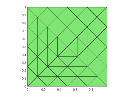
Figure 1: Triangular Mesh

Figure 2: Square Mesh

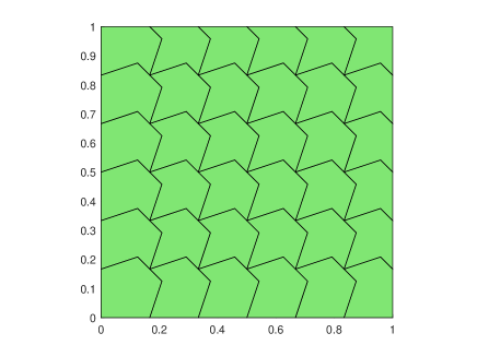
Figure 3: Concave Mesh

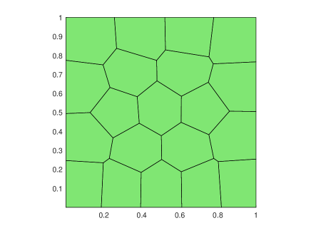
Figure 4: Structured Voronoi Mesh

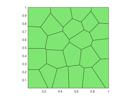
Figure 5: Random Voronoi Mesh

Figure 6: Triangular Mesh

6.1 Example on the square domain

Let the computational domain be $\Omega=(0,1)^{2}$ and the exact solution be given by $u=x^{2}y^{2}(1-x)^{2}(1-y)^{2}$ and $v=\sin^{2}(\pi x)\sin^{2}(\pi y)$. Then the right hand side load functions are computed as $f=\Delta^{2}u-[u,v]$ and $g=\Delta^{2}v+\frac{1}{2}[u,u]$. A series of triangular, square, concave, structured Voronoi, and random Voronoi meshes (see Figure 6-6) are employed to test the convergence results for the VEM. We observe in this example that the Newtons’ method converges in three iterations with a tolerance level of $10^{-8}$.

Table 1-5 show errors and orders of convergence for the displacement $u$ and the Airy-stress function $v$ for the aforementioned five types of meshes. Observe that linear order of convergences are obtained for $u$ and $v$ in the energy norm, and quadratic order of convergence in $L^{2}$ and $H^{1}$ norms, see Tables 1-4. These numerical order of convergence clearly matches the expected order of convergence given in (5.5), Theorems 5.2, and 5.3.

Table 1: Convergence results, Square domain, Triangular mesh

$h$	${\rm err}(u)$	Order	${\rm err}(\nabla u)$	Order	${\rm err}(Hu)$	Order
0.500000	0.003848	-	0.010163	-	0.087728	-
0.250000	0.000919	2.0659	0.002565	1.9864	0.040578	1.1123
0.125000	0.000248	1.8892	0.000730	1.8124	0.020991	0.9509
0.062500	0.000064	1.9633	0.000191	1.9382	0.010621	0.9829
0.031250	0.000016	1.9900	0.000048	1.9831	0.005328	0.9954

$h$	${\rm err}(v)$	Order	${\rm err}(\nabla v)$	Order	${\rm err}(Hv)$	Order
0.500000	0.767727	-	2.122015	-	19.371564	-
0.250000	0.177680	2.1113	0.567581	1.9025	9.503684	1.0274
0.125000	0.048263	1.8803	0.161082	1.8170	5.054876	0.9108
0.062500	0.012392	1.9615	0.041987	1.9398	2.575889	0.9726
0.031250	0.003121	1.9895	0.010620	1.9832	1.294492	0.9927

Table 2: Convergence results, Square domain, Square mesh

$h$	${\rm err}(u)$	Order	${\rm err}(\nabla u)$	Order	${\rm err}(Hu)$	Order
0.176777	0.002259	-	0.004788	-	0.037658	-
0.088388	0.000728	1.6342	0.001567	1.6117	0.014181	1.4089
0.044194	0.000198	1.8802	0.000439	1.8353	0.005473	1.3736
0.022097	0.000051	1.9632	0.000115	1.9388	0.002382	1.1200
0.011049	0.000013	1.9899	0.000029	1.9818	0.001134	1.0706

$h$	${\rm err}(v)$	Order	${\rm err}(\nabla v)$	Order	${\rm err}(Hv)$	Order
0.176777	0.340448	-	0.647508	-	7.335924	-
0.088388	0.109373	1.6382	0.194961	1.7317	2.871195	1.3533
0.044194	0.029214	1.9045	0.050934	1.9365	1.130682	1.3445
0.022097	0.007421	1.9769	0.012843	1.9876	0.507089	1.1569
0.011049	0.001862	1.9944	0.003216	1.9975	0.245155	1.0485

Table 3: Convergence results, Square domain, Concave mesh

$h$	${\rm err}(u)$	Order	${\rm err}(\nabla u)$	Order	${\rm err}(Hu)$	Order
0.242956	0.006516	-	0.011816	-	0.043874	-
0.121478	0.001881	1.7929	0.003695	1.6772	0.020415	1.1037
0.060739	0.000520	1.8534	0.001120	1.7215	0.008999	1.1818
0.030370	0.000138	1.9118	0.000319	1.8141	0.003882	1.2130
0.015185	0.000036	1.9570	0.000085	1.9089	0.001727	1.1686

$h$	${\rm err}(v)$	Order	${\rm err}(\nabla v)$	Order	${\rm err}(Hv)$	Order
0.242956	0.985669	-	2.021104	-	7.247490	-
0.121478	0.313766	1.6514	0.644574	1.6487	3.459449	1.0669
0.060739	0.086675	1.8560	0.179839	1.8416	1.548383	1.1598
0.030370	0.022635	1.9370	0.047895	1.9088	0.721287	1.1021
0.015185	0.005770	1.9720	0.012390	1.9507	0.346804	1.0565

Table 4: Convergence results, Square domain, Structured Voronoi Mesh

$h$	${\rm err}(u)$	Order	${\rm err}(\nabla u)$	Order	${\rm err}(Hu)$	Order
0.340697	0.005826	-	0.011623	-	0.071067	-
0.171923	0.002225	1.4075	0.004481	1.3935	0.030928	1.2164
0.083555	0.000650	1.7061	0.001476	1.5390	0.013413	1.1578
0.047445	0.000213	1.9673	0.000537	1.7855	0.006463	1.2900
0.027786	0.000074	1.9693	0.000195	1.8969	0.003328	1.2404

$h$	${\rm err}(v)$	Order	${\rm err}(\nabla v)$	Order	${\rm err}(Hv)$	Order
0.340697	0.906489	-	2.598308	-	10.88671	-
0.171923	0.370324	1.3089	0.935058	1.4943	4.857832	1.1798
0.083555	0.110610	1.6747	0.267744	1.7332	2.300755	1.0358
0.047445	0.035905	1.9881	0.091163	1.9037	1.187114	1.1692
0.027786	0.012727	1.9384	0.033555	1.8680	0.654228	1.1136

Table 5: Convergence results, Square domain, Random Voronoi Mesh

$h$	${\rm err}(u)$	Order	${\rm err}(\nabla u)$	Order	${\rm err}(Hu)$	Order
0.373676	0.006044	-	0.012864	-	0.072629	-
0.174941	0.002051	1.4240	0.004305	1.4422	0.028624	1.2269
0.089478	0.000502	2.1000	0.001204	1.9008	0.011996	1.2972
0.041643	0.000109	1.9973	0.000285	1.8855	0.004432	1.3017
0.020068	0.000035	1.5357	0.000095	1.4965	0.002194	0.9631

$h$	${\rm err}(v)$	Order	${\rm err}(\nabla v)$	Order	${\rm err}(Hv)$	Order
0.373676	0.871569	-	2.513214	–	10.518042	-
0.174941	0.350708	1.1995	0.912492	1.3349	4.654239	1.0743
0.089478	0.086986	2.0795	0.223585	2.0977	2.118548	1.1739
0.041643	0.018494	2.0243	0.049397	1.9741	0.856600	1.1839
0.020068	0.006145	1.5093	0.016285	1.5201	0.447808	0.8885

6.2 Example on the L-shaped domain

Consider the L-shaped domain $\Omega=(-1,1)^{2}\setminus\big{(}[0,1)\times(-1,0]\big{)}$. Choose the right hand functions such that the exact singular solution [27] in polar coordinates is given by

$$u=v=(r^{2}\cos^{2}\theta-1)^{2}(r^{2}\sin^{2}\theta-1)^{2}r^{1+\alpha}g_{\alpha,\omega}(\theta),$$

where $\alpha\approx 0.5444837367$ is a non-characteristic root of $\sin^{2}(\alpha\omega)=\alpha^{2}\sin^{2}(\omega)$, $\omega=\frac{3\pi}{2}$, and $g_{\alpha,\omega}(\theta)=(\frac{1}{\alpha-1}\sin((\alpha-1)\omega)-\frac{1}{\alpha+1}\sin((\alpha+1)\omega))(\cos((\alpha-1)\theta)-\cos((\alpha+1)\theta))$ $-(\frac{1}{\alpha-1}\sin((\alpha-1)\theta)-\frac{1}{\alpha+1}\sin((\alpha+1)\theta))(\cos((\alpha-1)\omega)-\cos((\alpha+1)\omega)).$ The computation of the discrete solution is executed utilizing triangular meshes, as depicted in Figure 6. In this example, the Newtons’ method exhibits convergence within four iterations, while maintaining a tolerance threshold of $10^{-8}$.

This example is particularly interesting since the solution is less regular due to the corner singularity. Since $\Omega$ is non-convex, we expect only sub-optimal order of convergences in the energy, $H^{1}$ and $L^{2}$ norms. Table 6 confirms these estimates numerically. A similar observation for Morley nonconforming FEM is present in [33, Section 5] and [26, Section 6.2.2] for a different weak formulation.

Table 6: Convergence results, L-shaped domain, Triangular mesh

$h$	${\rm err}(u)$	Order	${\rm err}(\nabla u)$	Order	${\rm err}(Hu)$	Order
0.707107	1.515408	-	3.748752	-	20.463977	-
0.353553	0.474713	1.6746	1.189979	1.6555	11.578325	0.8217
0.176777	0.135893	1.8046	0.347020	1.7778	6.166005	0.9090
0.088388	0.039031	1.7998	0.101701	1.7707	3.209604	0.9419
0.044194	0.011978	1.7042	0.033175	1.6162	1.682817	0.9315
0.022097	0.004070	1.5574	0.012555	1.4018	0.905976	0.8933

$h$	${\rm err}(v)$	Order	${\rm err}(\nabla v)$	Order	${\rm err}(Hv)$	Order
0.707107	1.035284	-	2.458626	-	15.791769	-
0.353553	0.431224	1.2635	1.084192	1.1812	11.359452	0.4753
0.176777	0.124537	1.7919	0.319836	1.7612	6.205400	0.8723
0.088388	0.035117	1.8263	0.091430	1.8066	3.236073	0.9393
0.044194	0.010510	1.7405	0.029067	1.6533	1.696020	0.9321
0.022097	0.003484	1.5929	0.010896	1.4156	0.912122	0.8949

Acknowledgements. The first author thanks Indian Institute of Space Science and Technology (IIST) for the financial support towards the research work. The second author thanks the Department of Science and Technology (DST-SERB), India, for supporting this work through the core research grant CRG/2021/002410.