Enabling Runtime Verification of Causal Discovery Algorithms with Automated Conditional Independence Reasoning
(Extended Version)

Abstract.

Causal discovery is a powerful technique for identifying causal relationships among variables in data. It has been widely used in various applications in software engineering. Causal discovery extensively involves conditional independence (CI) tests. Hence, its output quality highly depends on the performance of CI tests, which can often be unreliable in practice. Moreover, privacy concerns arise when excessive CI tests are performed.

Despite the distinct nature between unreliable and excessive CI tests, this paper identifies a unified and principled approach to addressing both of them. Generally, CI statements, the outputs of CI tests, adhere to Pearl’s axioms, which are a set of well-established integrity constraints on conditional independence. Hence, we can either detect erroneous CI statements if they violate Pearl’s axioms or prune excessive CI statements if they are logically entailed by Pearl’s axioms. Holistically, both problems boil down to reasoning about the consistency of CI statements under Pearl’s axioms (referred to as CIR problem).

We propose a runtime verification tool called CICheck, designed to harden causal discovery algorithms from reliability and privacy perspectives. CICheck employs a sound and decidable encoding scheme that translates CIR into SMT problems. To solve the CIR problem efficiently, CICheck introduces a four-stage decision procedure with three lightweight optimizations that actively prove or refute consistency, and only resort to costly SMT-based reasoning when necessary. Based on the decision procedure to CIR, CICheck includes two variants: ED-Check and P-Check, which detect erroneous CI tests (to enhance reliability) and prune excessive CI tests (to enhance privacy), respectively. We evaluate CICheck on four real-world datasets and 100 CIR instances, showing its effectiveness in detecting erroneous CI tests and reducing excessive CI tests while retaining practical performance.

1. Introduction

Causality analysis has become an increasingly popular methodology for solving a variety of software engineering problems, such as software debugging (Attariyan and Flinn, 2008; Xu and Zhou, 2015; Fariha et al., 2020; Dubslaff et al., 2022), performance diagnosis (Chen et al., 2014; Yoon et al., 2016), DNN testing, repairing, and explanations (Zhang and Sun, 2022; Sun et al., 2022; Ji et al., 2023b). It has also been successfully adopted in many other important domains, such as medicine (Pinna et al., 2010), economics (Addo et al., 2021), and earth science (Runge et al., 2019), and data analytics (Ma et al., 2023).

Causal discovery is the core technique of causality analysis. It aims to identify causal relations among variables in data and establish a causal graph. As a result, its output constitutes the foundation of the entire causality analysis pipeline and downstream applications. Many causal discovery algorithms, such as PC (Spirtes et al., 2000) and FCI (Zhang, 2008), perform a series of conditional independence (CI) tests on the data and build the causal graph using rules. Thus, the output quality of causal discovery algorithms is highly dependent on the way CI tests are performed.

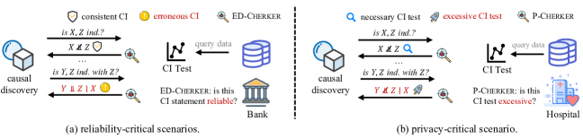
Figure 1. Two representative usage scenarios of causal discovery. “Ind.” denotes independence.

Reliability and Privacy. This research aims to enhance two key causal discovery scenarios: ➀ reliability-critical and ➁ privacy-critical. In the ➀ reliability-critical scenario (e.g., financial data processing), the focus is on the reliability of the causal discovery outputs. However, limited sample size or unsuitable statistical tests may impair CI test reliability. Unreliable CI tests may yield incorrect causal graphs, which undermines the credibility of causal discovery. To improve the reliability, we aim to ensure that all CI tests are consistent, a prerequisite for error-free causal discovery. In ➁ privacy-critical scenarios (e.g., health data processing), data privacy is typically a prime concern. In accordance to common privacy practices, access to data should be restricted unless necessary for causal discovery. Excessive CI tests may incur unnecessary data exposure and lead to a privacy concern. However, neither scenario has been thoroughly studied or addressed in the literature.

Conceptual Novelty. Our key insight is that we can address reliability and privacy concerns from CI tests in a unified way, by reasoning about the consistency of CI statements under the integrity constraint. We refer to this important task as Conditional Independence Reasoning (CIR). It’s important to note that CI statements within the same distribution comply with the well-established Pearl’s axioms, underpinned by statistical theories (Pearl and Paz, 1986). From this, we derive two key runtime verification strategies:

• In reliability-critical scenarios, we can detect erroneous outcomes of CI tests by checking whether the CI statements, derived from CI tests, comply with Pearl’s axioms. If not, we conclude that the CI statements contain errors and may need to abort the execution or alert users. Example: the red CI statement is erroneous in Fig. 1(a) because its negation is entailed by existing CI statements.

• In privacy-critical scenarios, we can prune excessive CI tests if their outcomes can be logically entailed by prior CI statements (under Pearl’s axioms). Example: the red CI statement is confirmed without incurring data access in Fig. 1(b), because it can be entailed by prior CI statements.

Technical Pipeline. It is evident that the above validation schemes can be integrated into existing causal discovery algorithms during runtime. Drawing upon the successful application of Runtime Verification (RV) tools in software security (e.g., preventing memory errors) (Chen et al., 2016; Roşu et al., 2009), we design a novel runtime verification tool, namely CICheck, to harden the reliability and privacy of causal discovery algorithms. At the heart of CICheck is an SMT-based reasoning system aligned with Pearl’s axioms, which facilitates consistency checking in CI statements. CICheck comprises two variants, ED-Check and P-Check, each employing different approaches to enhance common causal discovery algorithms in accordance with reliability-critical and privacy-critical usage scenarios, respectively.

However, efficiently implementing CICheck is challenging. First, CIR involves reasoning about first-order constraints, and while there are many off-the-shelf constraint solvers, adapting them to solve CIR problems is difficult. The challenge lies in encoding the problems soundly and compactly, while ensuring the encoded formulas are decidable. Second, the scope of all CI statements is significantly large, reaching up to $O(3^{n})$ for problems involving $n$ variables. This exponential increase in CI statements contributes to considerable overhead for SMT solving. To address the first challenge, we introduce a sound and decidable encoding scheme that translates CIR into SMT problems. To address the second challenge, we design a four-stage decision procedure as a backend for CICheck to solve CIR problems. Crucially, we design three lightweight optimizations that actively prove or refute consistency, and only resort to the costly SMT-based reasoning for instances when these strategies don’t yield a definitive resolution.

We evaluated the ED-Check and P-Check variants of CICheck on four real-world datasets and three synthetic datasets encompassing thousands of CI tests. The result shows the effectiveness of ED-Check in detecting erroneous CI tests and P-Check in pruning excessive CI tests and reducing privacy breaches significantly. We also evaluate 100 synthetic instances of the CIR problem and observe that our proposed optimization schemes make the expensive, nearly intractable SMT-based reasoning in CICheck feasible in practice. Our optimizations eliminate over 90% of SMT solving procedures and substantially cut down the execution time. In summary, we present the following contributions:

• Given the prosperous success of causal discovery algorithms, we advocate validating and augmenting causal discovery algorithms with runtime verification techniques in terms of both reliability and privacy. This contribution effectively broadenes the methodological horizon of formal methods while addressing emerging needs in causal inference.

• Our proposed solution, CICheck, is rigorously established based on Pearl’s axioms. It offers a sound, complete, and decidable runtime verification framework for causal discovery algorithms. To improve performance, we present a four-stage decision procedure including SMT-based solving and three optimizations.

• We evaluate CICheck on four real-world datasets and 100 synthetic instances of the CIR problem. The results show that CICheck can effectively detect erroneous CI tests and reduce excessive CI tests. Moreover, the synergistic use of our optimizations makes solving the CIR problem highly practical. CICheck is publicly available at an anonymous repository (art, 2023).

Potential Impact. We have disseminated our findings with multiple researchers from the causality community and received positive feedbacks. To quote one of their remarks (the developer of causal-learn (cau, 2023)), “it is indeed an awesome tool and we believe that it could definitely benefit the community a lot.” This underscores our work’s prospective influence on the broader research community.

2. Background

Notations. We denote a random variable by a capital letter, e.g., $X$, and denote a set of random variables by a bold capital letter, e.g., $\bm{X}$. We use $\bm{V}$ to denote the set of all random variables. As a slight abuse of notation, depending on the context, we also use a capital letter $X$ or a bold capital letter $\bm{X}$ to denote a node or a set of nodes in the causal graph, respectively. We use $\bm{X}\Perp\bm{Y}\mid\bm{Z}$ to represent a general CI relationship and use $\bm{X}\Perp_{G}\bm{Y}\mid\bm{Z}$ to represent d-separation (i.e., a graphical separation criterion in a graph (Spirtes et al., 2000); see details in Sec. A of Supp. Material). A statement of conditional independence/dependence is represented by lower Greek letters, e.g., $\tau\coloneqq(\bm{X}\Perp\bm{Y}\mid\bm{Z})$ or $\rho\coloneqq(\bm{X}\not\Perp\bm{Y}\mid\bm{Z})$. We also use dependent/independent CI statements to refer to the above two classes of statements. We use $\models$ to denote semantical entailment and $\neg$ to denote negation. For instance, if $\tau\coloneqq(\bm{X}\Perp\bm{Y}\mid\bm{Z})$, then $\neg\tau\models(\bm{X}\not\Perp\bm{Y}\mid\bm{Z})$. We use $\Sigma$ to denote a set of CI statements and $\Phi$ to denote Pearl’s axioms. And, we use KB to denote a knowledge base built on $\Sigma$ and $\Phi$. $\textit{KB}\models\bot$ indicates that it is inconsistent.

2.1. CI & Pearl’s Axioms

Definition 2.0 (Conditional Independence and Dependence).

Let $\bm{X},\bm{Y},\bm{Z}\subseteq\bm{V}$ be three disjoint sets of random variables from domain $\bm{V}$. We say that $\bm{X}$ and $\bm{Y}$ are conditionally independent given $\bm{Z}$ (denoted by $\bm{X}\Perp\bm{Y}\mid\bm{Z}$) if and only if $P(\bm{Z})>0$ and

(1) $$\small P(\bm{X},\bm{Y}\mid\bm{Z})=P(\bm{X}\mid\bm{Z})P(\bm{Y}\mid\bm{Z})$$

We say that $\bm{X}$ and $\bm{Y}$ are conditionally dependent given $\bm{Z}$ (denoted by $\bm{X}\not\Perp\bm{Y}\mid\bm{Z}$) if and only if $P(\bm{Z})>0$ and

(2) $$\small P(\bm{X},\bm{Y}\mid\bm{Z})\neq P(\bm{X}\mid\bm{Z})P(\bm{Y}\mid\bm{Z})$$

Empirically, statistical tests like $\chi^{2}$-squared test examine CI. Like many statistical tests, a $p$-value indicates the error probability when rejecting the null hypothesis. Here, the null hypothesis assumes conditional independence between $\bm{X}$ and $\bm{Y}$ given $\bm{Z}$. Typically, the null hypothesis is rejected if $p$-value $<1-\alpha$ ($\alpha$ is the level of significance). A $p$-value$<1-\alpha$ rejects the null hypothesis, implying $\bm{X}\not\Perp\bm{Y}\mid\bm{Z}$. Otherwise, $\bm{X}\Perp\bm{Y}\mid\bm{Z}$.

Beyond CI tests on empirical distribution, efforts are made to axiomatize CI statements based on their mathematical definition. Pearl’s axioms are well-known rules that specify the integrity constraint of CI statements within a domain (Pearl, 1988). They can be represented as Horn clauses over a class of probability distributions $\mathcal{P}$ to verify them (Geiger and Pearl, 1993). Here, we use $\mathcal{P}$ to denote the universal set of probability distributions of interest. In particular, we consider probability distributions over faithful Bayesian networks (a standard setup in causality analysis (Spirtes et al., 2000)). Intuitively, it implies the correspondence between CI in the probability distribution and the graphical structure (see the definition in Sec. A of Supp. Material). We present Pearl’s axioms in the form of Horn clauses as follows.

Symmetry.

(3) $$\small(\bm{X}\Perp\bm{Y}\mid\bm{Z})\iff(\bm{Y}\Perp\bm{X}\mid\bm{Z})$$

Decomposition.

(4) $$(\bm{X}\Perp\bm{Y}\cup\bm{W}\mid\bm{Z}) \implies(\bm{X}\Perp\bm{Y}\mid\bm{Z})$$

Weak Union.

(5) $$\small(\bm{X}\Perp\bm{Y}\cup\bm{W}\mid\bm{Z})\implies(\bm{X}\Perp\bm{Y}\mid\bm{Z}\cup\bm{W})$$

Contraction.

(6) $$\small(\bm{X}\Perp\bm{Y}\mid\bm{Z})\land(\bm{X}\Perp\bm{W}\mid Z\cup\bm{Y})\implies(\bm{X}\Perp\bm{Y}\cup\bm{W}\mid\bm{Z})$$

Intersection.

(7) $$\small(\bm{X}\Perp\bm{Y}\mid\bm{Z}\cup\bm{W})\land(\bm{X}\Perp\bm{W}\mid\bm{Z}\cup\bm{Y})\implies(\bm{X}\Perp\bm{Y}\cup\bm{W}\mid\bm{Z})$$

Composition.

(8) $$\small(\bm{X}\Perp\bm{Y}\mid\bm{Z})\land(\bm{X}\Perp\bm{W}\mid\bm{Z})\implies(\bm{X}\Perp\bm{Y}\cup\bm{W}\mid\bm{Z})$$

Weak Transitivity.

(9) $$(\bm{X}\Perp\bm{Y}\mid\bm{Z})\land(\bm{X}\Perp\bm{Y}\mid\bm{Z}\cup\{U\}) \implies(U\Perp\bm{Y}\mid\bm{Z})$$

Chordality.

(10) $$(X\Perp Y\mid\{Z,W\})\land(Z\Perp W\mid\{X,Y\}) \implies(X\Perp Y\mid Z)$$

$X,Y,Z,W,U$ are single variables in Eqn. 9 and Eqn. 10.

CI Axioms vs. CI Tests. The above properties are termed axioms as, considering certain assumptions such as faithful Bayesian networks, there are no probability distributions that contradict them. They essentially serve as integrity constraints useful in refuting inaccurate CI statements. However, they are not sufficient to deduce whether a CI statement is correct because axioms are subject to the whole class of probability distributions while the correctness of a CI statement is only concerned with a specific distribution. In other words, these CI statements can only be examined by CI tests on a particular probability distribution. In this regard, a CI test can be deemed an oracle to CI statements. Theoretically, CI tests are asymptotically accurate although they may be inaccurate with finite samples. Due to inaccuracy, the axioms may be violated. The reliability- and privacy-enhancing variants of CICheck (ED-Check and P-Check) aim to ➀ check if a CI statement obtained by CI tests complies with Pearl’s axioms, and ➁ prune excessive CI tests that are directly entailed by CI axioms.

2.2. Constraint-based Causal Discovery

In this section, we briefly introduce the application of CICheck, i.e., causal discovery. Causal discovery aims to learn causal relations from observational data and is a fundamental problem in causal inference. It has been widely adopted in many fields. Causal relations among data are represented in the form of a directed acyclic graph (DAG), where the nodes are constituted by all variables $\bm{V}$ in data and an edge $X\to Y$ in the DAG indicates a cause-effect relation between the parent node $X$ and the child node $Y$.

Constraint-based causal discovery is the most classical approach to identifying the causal graph (precisely, its Markov equivalence class) from observational data (Spirtes et al., 2000). It is based on the assumptions below that affirm the equivalence between CI and d-separation.

Definition 2.0 (Global Markov Property (GMP)).

Given a distribution $P_{\bm{V}}$ and a DAG $G$, $G$ is said to be faithful to $P_{\bm{V}}$ if $X\Perp_{G}Y\mid Z\implies X\Perp Y\mid Z$.

Definition 2.0 (Faithfulness).

Given a distribution $P_{\bm{V}}$ and a DAG $G$, $P_{\bm{V}}$ is said to satisfy GMP relative to $G$ if $X\Perp Y\mid Z\implies X\Perp_{G}Y\mid Z$.

Peter-Clark (PC) Algorithm. To practically identify the causal graph under the above assumptions, the PC algorithm is the most widely used. The PC algorithm, a prominent causal discovery approach (Spirtes et al., 2000), consists of two principal stages: (1) skeleton identification and (2) edge orientation. In the first stage, the algorithm starts from a fully connected graph, iteratively searches for separating sets ($\bm{Z}$) that d-separate nodes, consequently removing associated edges. To expedite this process, a greedy strategy is implemented. In the second stage, edge orientations are determined according to specific criteria (see the full algorithm in Sec. C of Supp. Material). When Def. 2.2 and Def. 2.3 hold and CI tests are correct, the PC algorithm is guaranteed to identify a genuine causal graph. From a holistic view, one can comprehend the PC algorithm as iteratively executing a series of CI tests, which aims to construct a causal graph with pre-defined rules and results of CI tests.

3. Research Overview

In this section, we present an illustrative example to show how CICheck can be reduced to CIR problem solving. Then, we formulate the CIR problem and show how to connect it with CICheck.

3.1. Illustrative Example

We present a case in accordance with Fig. 1 where ED-Check detects an erroneous CI statement in the PC algorithm. To ease presentation, we analyze the case from the view of ED-Check while the procedure also applies to P-Check.

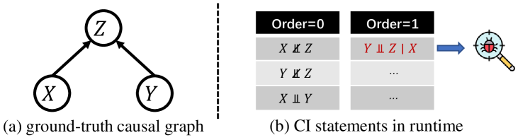
Figure 2. An erroneous CI statement occurred when launching the PC algorithm.

Consider a set of random variables $\bm{V}=\{X,Y,Z\}$ whose ground-truth causal graph is shown in Fig. 2(a). The PC algorithm aims to identify the causal structure from the dataset corresponding to $\bm{V}=\{X,Y,Z\}$. When $\textit{order}=0$, the algorithm enumerates all (pairwise) marginal independence relations. As shown in the left-side table in Fig. 2(b), it identifies that $\{(X\not\Perp Z),(Y\not\Perp Z),(X\Perp Y)\}$. Since $Y\not\Perp Z$, when $\textit{order}=1$, the PC algorithm would further query whether $Y\Perp Z\mid X$ holds by invoking a CI test. However, due to errors occurred in the current CI test, $\sigma=Y\Perp Z\mid X$ is deemed true. Hence, the PC algorithm incorrectly concludes that $Y$ and $Z$ are non-adjacent, and yields an erroneous causal graph accordingly.

The above error is detectable under Pearl’s axioms: $\neg\sigma$ can be logically entailed by considering the marginal CI statements (shown in the left-side table of Fig. 2(b)) and Pearl’s axioms, which can be proved easily by contradiction. Consider the proof below:

Proof.

Suppose $Y\Perp Z\mid X$ is true. By Contraction axiom, $Y\Perp Z\mid X$ and $X\Perp Y$ implies that $Y\Perp\{X,Z\}$. Then, by Decomposition axiom, $Y\Perp\{X,Z\}$ implies that $Y\Perp X$ and $Y\Perp Z$. This contradicts the fact that $X\not\Perp Y$. ∎

Therefore, $\sigma$ is not warranted by Pearl’s axioms and we can flag it as inconsistent.

Extension to P-Check. Similar to earlier case, P-Check preempts CI testing by concurrently validating if $Y\Perp Z\mid X$ or $Y\not\Perp Z\mid X$ is warranted. Given that Pearl’s axioms only warrant $Y\not\Perp Z\mid X$, we directly infer $Y\not\Perp Z\mid X$ as the correct statement. Besides, inaccurate CI tests may undermine the effectiveness of P-Check. We discuss this issue in Sec. 5 and Sec. 6.5.

3.2. Problem Statement

The CIR Problem. The above reasoning process in the proof is ad-hoc. To deliver an automated reasoning-based runtime verification, we need a general reasoning tool to automate the above process. We define the following problem (Conditional Independence Reasoning; CIR) to formalize the above reasoning process.

If the CIR problem returns a true value, we conclude that there is an inconsistency error among $\Sigma$ under Pearl’s axioms. Otherwise, $\Sigma$ is consistent under Pearl’s axioms.

Building CICheck via CIR Reasoning Fig. 1 illustrates two typical and representative usage scenarios of CICheck, in the form of reliability- and privacy-enhancing variants, ED-Check and P-Check, respectively. We hereby build them, by recasting their specific objective into one (or multiple) instances of the CIR problem. In this way, the two variants of CICheck can be implemented in a unified manner. Alg. 1 presents the algorithmic details of CICheck.

Input: Variable Pair $X,Y$, Condition Set $\bm{Z}$

Output: $X\Perp Y\mid\bm{Z}$ or $X\not\Perp Y\mid\bm{Z}$

1 Function ED-Check ($X,Y,\bm{Z}$):

2       $\gamma\leftarrow\textit{CITest}(X,Y,\bm{Z})$;

3       $\texttt{assert}~{}\textit{KB}\coloneq\{\Sigma\cup\{\gamma\},\Phi\}\not\models\bot$;

4       return $\gamma$;

5      

6Function P-Check ($X,Y,\bm{Z}$):

7       $\gamma\leftarrow X\Perp Y\mid\bm{Z}$;

8       if $\textit{KB}\coloneq\{\Sigma\cup\{\gamma\},\Phi\}\models\bot$ then

9             return $X\not\Perp Y\mid\bm{Z}$

10       else if $\textit{KB}\coloneq\{\Sigma\cup\{\neg\gamma\},\Phi\}\models\bot$ then

11             return $X\Perp Y\mid\bm{Z}$

12       else

13            return $\textit{CITest}(X,Y,\bm{Z})$

Algorithm 1 Two variants of CICheck

ED-Check initiates the CI test (line 2), obtaining the output CI statement $\gamma$. It then checks if $\gamma$ is consistent under Pearl’s axioms (line 3), ensuring that $\textit{KB}\coloneq{\Sigma\cup{\gamma},\Phi}\not\models\bot$. If $\textit{KB}\models\bot$, ED-Check can either abort execution or notify the user. In this way, ED-Check can detect erroneous CI statements.

P-Check checks the consistency of both $X\Perp Y\mid\bm{Z}$ and $X\not\Perp Y\mid\bm{Z}$ under Pearl’s axioms. In particular, before conducting the CI test (line 12; which accesses the private user data), P-Check first checks whether the incoming CI statement can be deduced from the existing CI statements (lines 7 and 9). If it is deducible, we omit the CI test and directly return the deduced CI statement (lines 8 and 10). Otherwise, we resort to the CI test (line 12). Hence, there is at most one CI test performed throughout the process.

Notably, P-Check reduces privacy leakage by pruning unnecessary CI tests. This is because eliminating a CI test prevents access to its associated private data. For instance, in a hospital scenario, we may deduce one CI relation among multiple diseases (e.g., $D_{1}\not\Perp D_{2}\mid D_{3}$) from the existing CI statements (e.g., $D_{1}\not\Perp D_{2}$, $D_{1}\Perp D_{3}$ and $D_{2}\not\Perp D_{3}$). This eliminates the need to access the private information of $D_{1}\not\Perp D_{2}\mid D_{3}$.

Challenges. While the CIR problem appears simple, solving it efficiently is far from trivial. On a theoretical level, it requires a sound, compact, and decidable encoding scheme to convert the CIR problem into an SMT problem. Practically speaking, the states of CI statements can be overwhelming, resulting in as many as $O(3^{n})$ CI statements for problems involving $n$ variables. This exponential growth can result in significant overhead for SMT solving and make solving complex CIR problems impractical. Next, we show how these technical challenges are addressed in Sec. 4.

4. Automated Reasoning for CIR

This section presents an automated reasoning framework for solving any instances of the CIR problem (defined in Sec. 3). We first show how CIR can be formulated as an SMT problem, and present a decidable, SMT-based encoding scheme to the problem. We then present several optimizations to boost the solving of this problem, which makes it practical in real-world usage.

4.1. Encoding the CIR Problem

Formulation. Our research leverages the observation that the CIR problem, based on Pearl’s axioms, can translate to a satisfiability issue. Consider an instance of the CIR problem; we expect the solver to verify whether $\langle\Sigma,\Phi\rangle\coloneqq\bigwedge\limits_{i=1}^{k}\sigma_{i}\wedge\bigwedge\limits_{j=1}^{m}\Phi_{j}$ is satisfiable, where $\sigma_{i}$ is a CI statement and $\Phi_{j}$ is a rule of Pearl’s axioms. If the formula is unsatisfiable, we can conclude that the CIR instance yields a contradiction (i.e., $\textit{KB}\models\bot$).

Example 4.0.

Consider the example in Fig. 2. The CIR problem is to check whether the following formula is satisfiable:

(11) $$\small\{X\not\Perp Z\}\wedge\{Y\not\Perp Z\}\wedge\{X\Perp Y\}\wedge\{Y\Perp Z\mid X\}\wedge\bigwedge\limits_{j=1}^{m}\Phi_{j}$$

where $\Phi_{j}$ represents a rule of Pearl’s axioms. If the formula is unsatisfiable, then the CI statements are inconsistent under Pearl’s axioms.

Despite the simplicity of the procedure above, it is non-trivial to automatically reason about the satisfiability of $\langle\Sigma,\Phi\rangle$ in a sound, decidable, and efficient manner. First, the space of all possible CI statements should be appropriately modeled, where unseen CI statements are also considered. It is noteworthy that, while addressing the consistency of CI statements, some (intermediate) CI statements do not necessarily appear in the set. We present an example in Sec. 3.1 to illustrate this. The check process first deduces an unseen CI statement (i.e., $Y\Perp{X,Z}$). Then, it uses this previously unseen CI statement to refute the consistency. Consequently, simply ignoring unseen CI statements may lead to an incorrect result. Second, since CI statements are defined on three sets of variables (i.e., $\bm{X},\bm{Y},\bm{Z}$), an efficient encoding of sets and their primitives is necessary. Third, we need to encode Pearl’s axioms as quantified first-order formulas. We address them in what follows.

Modeling CI Statements. We first show how to model all possible CI statements as SMT formulas, including potentially unseen CI statements in $\Sigma$. We utilize the theory of Equality with Uninterpreted Functions (EUF) (Ackermann, 1954; Kroening and Strichman, 2016) for this modeling. EUF extends the Boolean logic with equality predicates in the form of $\texttt{UF}(x)=y$, where UF is an uninterpreted function symbol. Notably, UF adheres to the axiom of functional congruence, implying identical inputs yield identical outputs (for instance, $x=y\land\texttt{UF}(x)\neq\texttt{UF}(y)$ is unsatisfiable). This inherent feature holds importance in CI statement encoding as it guarantees their invariance for fixed $\bm{X},\bm{Y},\bm{Z}$. Besides, modern SMT solvers for the EUF theory have efficient enforcement for the functional congruence axiom.

Hence, the characteristics of the EUF theory make it both suitable and practical to model CI statements. An uninterpreted function symbol $\texttt{CI}:2^{\bm{V}}\times 2^{\bm{V}}\times 2^{\bm{V}}\to{0,1}^{2}$ is defined, having three arguments $\bm{X},\bm{Y},\bm{Z}$ that are $\bm{V}$’s subsets. $\texttt{CI}(\bm{X},\bm{Y},\bm{Z})$ outputs a size-2 bit-vector ($b_{n-1}\ldots b_{0}$, $b_{i}\in{0,1}$ sequence). The semantics of $\texttt{CI}(\bm{X},\bm{Y},\bm{Z})$’s outputs are defined next.

(12) $$\small\texttt{CI}(\bm{X},\bm{Y},\bm{Z})\coloneqq\begin{cases}\texttt{01}&\text{if }\bm{X}\Perp\bm{Y}\mid\bm{Z}\\ \texttt{00}&\text{if }\bm{X}\not\Perp\bm{Y}\mid\bm{Z}\\ \texttt{11}&\text{if }\bm{X},\bm{Y},\bm{Z}\text{ are invalid}\end{cases}$$

Here, we create an additional state $\texttt{CI}(\bm{X},\bm{Y},\bm{Z})=-1$ to ensure that the uninterpreted function CI is well-defined for all possible $\bm{X},\bm{Y},\bm{Z}$ inputs. $\bm{X},\bm{Y},\bm{Z}$ are invalid in the following case:

1. $\bm{X}\cap\bm{Y}\neq\emptyset$; or $\bm{X}\cap\bm{Z}\neq\emptyset$; or $\bm{Y}\cap\bm{Z}\neq\emptyset$.

2. $\bm{X}=\emptyset$; or $\bm{Y}=\emptyset$.

Representing Sets. Nevertheless, the argument types in the definition of CI given above — sets — are not supported in many state-of-the-art SMT solvers. The Z3 solver, a widely-used SMT solver with limited set support, relies on arrays to simulate sets and is inefficient. To overcome this, we use the bit-vector theory to deliver a compact and decidable encoding of $\bm{X},\bm{Y},\bm{Z}$, as well as set primitives and Pearl’s axioms over these variables.

We define a function set2vec that encodes each set variable into a bit-vector variable: $\texttt{set2vec}:2^{\bm{V}}\to\{0,1\}^{|\bm{V}|}$ Next, we use $BV_{\bm{X}},BV_{\bm{Y}},BV_{\bm{Z}}$ to represent the bit-vector variables corresponding to $\bm{X},\bm{Y},\bm{Z}$, respectively. The bit-vector variables $BV_{\bm{X}},BV_{\bm{Y}},BV_{\bm{Z}}$ can constitute the arguments of the uninterpreted function CI (with a slight abuse of notation, we “override” the symbol CI (Eqn. 12) and make it to take bit-vectors as input).

With the bit-vector representation of a set, we now encode set primitives using bit-vector operations:

(13) $$\small\bm{X}=\emptyset \iff BV_{\bm{X}}=\bm{0}$$

(14) $$|\bm{X}|=1 \iff\sum_{i=0}^{|\bm{V}|-1}\texttt{extract}(i,i,BV_{\bm{X}})=1$$

(15) $$\text{abbreviated to }|BV_{X}|=1$$

(16) $$\bm{X}\cup\bm{Y} \iff BV_{\bm{X}}\mathbin{|}BV_{\bm{Y}}$$

(17) $$\bm{X}\cap\bm{Y} \iff BV_{\bm{X}}\mathbin{\&}BV_{\bm{Y}}$$

(18) $$\bm{X}\subseteq\bm{Y} \iff BV_{\bm{X}}\mathbin{\&}BV_{\bm{Y}}=BV_{\bm{X}}$$

(19) $$X\in\bm{Y} \iff|BV_{X}|=1\land BV_{X}\mathbin{\&}BV_{\bm{Y}}=BV_{X}$$

Next, we show an instantiation of the encoding scheme.

Example 4.0.

Consider $\bm{V}=\{X,Y,Z\}$, $\bm{X}=\{X\}$, $\bm{Y}=\{Y\}$, and $\bm{Z}=\{Y\}$. Without loss of generality, we have $BV_{\bm{X}}=001$, $BV_{\bm{Y}}=010$, $BV_{\bm{Z}}=100$ and $BV_{\emptyset}=000$. Then, the CI statements in Example 4.1 where $\Sigma\coloneqq\{(X\not\Perp Z),(Y\not\Perp Z),(X\Perp Y),(Y\Perp Z\mid X)\}$ can be encoded as:

(20) $$\texttt{CI}(BV_{\bm{X}},BV_{\bm{Z}},BV_{\emptyset})=\texttt{CI}(\texttt{\text@underline{001}, \text@underline{100}, \text@underline{000}})=\texttt{00}$$

$$\texttt{CI}(BV_{\bm{Y}},BV_{\bm{Z}},BV_{\emptyset})=\texttt{CI}(\texttt{\text@underline{010}, \text@underline{100}, \text@underline{000}})=\texttt{00}$$

$$\texttt{CI}(BV_{\bm{X}},BV_{\bm{Y}},BV_{\emptyset})=\texttt{CI}(\texttt{\text@underline{001}, \text@underline{010}, \text@underline{000}})=\texttt{01}$$

$$\texttt{CI}(BV_{\bm{Y}},BV_{\bm{Z}},BV_{X})=\texttt{CI}(\texttt{\text@underline{010}, \text@underline{100}, \text@underline{001}})=\texttt{01}$$

As shown in Example 4.2, the CI statements are encoded as EUF constraints using bit-vector variables. Similarly, we can encode the other CI relations.

Encoding Axioms. We only apply Pearl’s axioms to valid arguments of the uninterpreted function CI. Therefore, prior to encoding Pearl’s axioms, we define the validity constraint to check whether the argument of CI is valid; these validity constraints form the premises of all axioms.

(21) Valid $$(BV_{\bm{X}},BV_{\bm{Y}},BV_{\bm{Z}})\coloneqq$$

$$BV_{\bm{X}}\mathbin{\&}BV_{\bm{Y}}=\bm{0}\land BV_{\bm{X}}\mathbin{\&}BV_{\bm{Z}}=\bm{0}$$

$$\land BV_{\bm{Y}}\mathbin{\&}BV_{\bm{Z}}=\bm{0}\land BV_{X}\neq\bm{0}\land BV_{\bm{Y}}\neq\bm{0}$$

Next, we encode Pearl’s axioms. For each rule, we create free-variables corresponding to the variables used in this rule, and use universal quantification to specify the rule in all possible concretization to these variables.

Example 4.0.

Consider the Decomposition axiom:

$$(\bm{X}\Perp\bm{Y}\cup\bm{W}\mid\bm{Z}) \implies(\bm{X}\Perp\bm{Y}\mid\bm{Z})$$

$$(\bm{X}\Perp\bm{Y}\cup\bm{W}\mid\bm{Z}) \implies(\bm{X}\Perp\bm{W}\mid\bm{Z})$$

We define the following constraint to encode the axiom (and we omit the validity constraint for ease of presentation).

(22) $$\forall BV_{\bm{X}},BV_{\bm{Y}},BV_{\bm{Z}},BV_{\bm{W}}\in\{0,1\}^{|\bm{V}|}$$

$$\texttt{CI}(BV_{\bm{X}},BV_{\bm{Y}}|BV_{\bm{W}},BV_{\bm{Z}})=\texttt{01}\implies\texttt{CI}(BV_{\bm{X}},BV_{\bm{Y}},BV_{\bm{Z}})=\texttt{01}$$

$$\texttt{CI}(BV_{\bm{X}},BV_{\bm{Y}}|BV_{\bm{W}},BV_{\bm{Z}})=\texttt{01}\implies\texttt{CI}(BV_{\bm{X}},BV_{\bm{W}},BV_{\bm{Z}})=\texttt{01}$$

In the above constraint, we first create a universal quantifier and four free bit-vector variables $BV_{\bm{X}}$, $BV_{\bm{Y}}$, $BV_{\bm{Z}},BV_{\bm{W}}$ corresponding to $\bm{X},\bm{Y},\bm{Z},\bm{W}$ respectively. Then, we create two implication constraints ($\implies$) corresponding to the two Horn clauses of the Decomposition axiom, where the set union is encoded as bitwise-or operations.

Similarly, we can encode the remaining axioms via universal quantifiers (see the encoding in Sec. B of Supp. Material).

Proposition 4.4.

The encoded SMT problem is a sound and complete representation of the CIR problem. And, the problem is decidable.

Proof Sketch.

Soundness & Completeness. Let’s consider an instance of CIR problem with $\Sigma$ being the set of CI statements and let $\phi_{c}$ be an oracle to CIR problem. Following the encoding procedure, we can construct an SMT problem with $\mathcal{C}$ being the constraints and let $\phi_{s}$ be an SMT solver. The soundness of the encoding scheme implies that if $\phi_{s}(\mathcal{T})$ returns satisfiable, then $\phi_{c}(\Sigma)$ returns consistent. The completeness of the encoding scheme implies that if $\phi_{c}(\Sigma)$ returns consistent, then $\phi_{s}(\mathcal{T})$ returns satisfiable.

Lemma 4.5.

If there exists a joint distribution $P$ that admits all CI statements in $\Sigma$, then $\Sigma$ is consistent.

Lemma 4.6.

If there does not exist a joint distribution $P$ that admits all CI statements in $\Sigma$, then $\Sigma$ is inconsistent.

Lemma 4.7.

There does not exist a joint distribution $P$ that simultaneously admits one CI statement and its negation.

Lemma 4.8.

Constraints only containing the Pearl’s axioms are always satisfiable.

Lemma 4.5 and Lemma 4.6 are direct consequences by the definition of Pearl’s axioms. Lemma 4.7 is a direct consequence of the definition of conditional independence (Eqn. 1 and Eqn. 2). Lemma 4.8 (i.e., self-consistency of Pearl’s axioms) can be derived from the graphical criterion of conditional independence (Pearl and Paz, 1986).

Assume that $\phi_{s}(\mathcal{T})$ is satisfiable. From this premise, it directly follows that there exists an uninterpreted function CI satisfying Pearl’s axioms. We define CI as in Eqn. 12, ensuring that it is well-defined for all potential inputs $\bm{X},\bm{Y},\bm{Z}$. Given the existence of CI, we can construct a corresponding direct acyclic graph (DAG) $G$ in accordance to the SGS algorithm (Spirtes et al., 2000). Then, based on the result of (MEEK, 1995), there exists a joint distribution $P$ that admits $G$. By Lemma 4.5, we affirm that the CI statements are consistent under Pearl’s axioms when the encoded SMT problem is satisfiable. Conversely, suppose that $\phi_{s}(\mathcal{T})$ is unsatisfiable. By Lemma 4.8, we know that the minimum unsatisfiable core contains at least one CI statement. Without loss of generality, we assume

$$\{\sigma_{i-1},\sigma_{i},\ldots,\sigma_{j},\Phi_{k},\ldots,\Phi_{l}\}$$

be the minimum unsatisfiable core of $\mathcal{T}$. We have

$$\{\sigma_{i},\ldots,\sigma_{j},\Phi_{k},\ldots,\Phi_{l}\}\models\neg\sigma_{i-1}$$

. In the meantime, we also have $\sigma_{i-1}$ in $\Sigma$. By Lemma 4.7, we know that there does not exist a joint distribution $P$ that simultaneously admits $\sigma_{i-1}$ and its negation. By Lemma 4.5, this indicates that the CI statements are inconsistent under Pearl’s axioms when the encoded SMT problem is unsatisfiable. Therefore, the encoded SMT problem gives a sound and complete representation of the CIR problem, which deals with the consistency of CI statements.

Decidability. In our encoded SMT problem, we find constraints that belong to the combined theory of uninterpreted functions and quantified bit-vectors. According to Wintersteiger et al. (Wintersteiger et al., 2013), it is known that this combined theory is decidable. This ensures the decidability of the constraints in our problem, hence confirming the decidability of the entire encoded SMT problem. ∎

4.2. Solving the CIR Problem

We describe the encoding of the CIR problem in Sec. 4.1. Despite the rigorously formed encoding, this approach is NEXP-complete (Wintersteiger et al., 2013), meaning that it may become intractable for complex problem instances. In this section, we present several optimizations and design choices to make CICheck practical at a moderate cost.

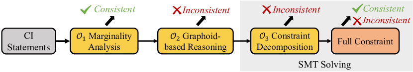
Figure 3. Overview of the CIR problem solving pipeline.

Fig. 3 outlines the workflow of our solving procedure. In short, before launching the SMT solver over the full constraint obtained by our encoding scheme, we leverage the following three lightweight optimizations to prove or refute the satisfiability of the constraint and presumably “early-stop” the reasoning to avoid costly SMT solving. Particularly, Marginality Analysis is performed first and can prove the satisfiability of the constraint. If Marginal Analysis fails, we then apply the following two optimizations (Graphoid-based Reasoning and Constraint Decomposition) to refute the satisfiability. SMT solving over the full constraint is only performed when none of the optimizations reaches a conclusive result.

4.2.1. $\mathcal{O}_{1}$ Marginality Analysis

In general, we need to check every CI test to ensure that each one is valid (or can be pruned), depending on the application. However, we notice that when $\Sigma$ only contains non-degenerate marginal CI statements, check is not necessary. The following theorem characterizes this property:

Theorem 4.9.

Let $\Sigma$ be a set of non-degenerate marginal CI statements. Here, $\Sigma$ is said to be non-degenerate if $\Sigma$ does not contain both a marginal CI statement and its negation. A marginal CI statement is a CI statement with an empty condition set, such as $X\Perp Y$. Then, $\Sigma$ is always consistent under Pearl’s axioms.

Proof Sketch.

By definition, $\Sigma$ is consistent under Pearl’s axioms if there exists a joint distribution $P$ such that $P$ admits every CI statement in $\Sigma$. Below, we demonstrate that such a joint distribution $P$ always exists for arbitrary $\Sigma$, as long as it only contains non-degenerate marginal CI statements. Let $G_{u}$ be an undirected graph where each node in $G_{u}$ represents a random variable with respect to $P$. Two nodes $X,Y$ are connected by an edge if and only if $X\not\Perp Y$. According to the “acyclic orientation” in (Stanley, 1973), any undirected graph can be converted to a directed acyclic graph (DAG). Let $G_{d}$ be a DAG of $G_{u}$. Then, according to Theorem 5 of (MEEK, 1995), a faithful multinomial $P$ exists for any DAG $G_{d}$. In this regard, $\Sigma$ is at least warranted in $P$ and is thus consistent. ∎

Theorem 4.9 directly implies we can omit CICheck, when $\Sigma$ exclusively holds non-degenerate marginal CI statements. Often, this occurs in the initial phases of common causal discovery algorithms, shown in the example below.

Example 4.0.

Consider the first three CI statements in Example 4.1, with $\Sigma\coloneqq{(X\not\Perp Z),(Y\not\Perp Z),(X\Perp Y)}$. As $\Sigma$ consists solely of non-degenerate marginal CI statements, according to Theorem 4.9, we can directly infer that $\Sigma$ is consistent.

4.2.2. $\mathcal{O}_{2}$ Graphoid-based Reasoning

In causal inference, CI statements are often represented as graphoids (Pearl and Paz, 1986), which are special graphical data structures that enable efficient reasoning about ➀ whether a CI statement is always independent. As a result, graphoid-based reasoning cannot distinguish “➁ a CI statement is always dependent” from “➂ a CI statement can be either independent or dependent”. Despite this limitation, graphoid-based reasoning is useful in our context owing to its efficiency. In practice, we find graphoid-based reasoning to be significantly faster than solving standard CIR problems. Below, we show the translation from an instance of the CIR problem to a sequence of graphoid-based reasoning.

Let the knowledge base $\Sigma=\{\sigma_{1},\ldots,\sigma_{k}\}$ be the input of a CIR problem. We split $\Sigma$ into two parts: (1) the first part, $\Sigma_{1}$, contains all dependent CI statements (e.g., $X\not\Perp Y\mid\bm{Z}$), and (2) the second part, $\Sigma_{2}$, contains all independent CI statements (e.g., $X\Perp Y\mid\bm{Z}$). We can then use graphoid-based reasoning to check if $\Sigma_{2}$ implies the negation of any instances in $\Sigma_{1}$ (e.g., $\Sigma_{2}\implies\neg\sigma_{i}$ where $\sigma_{i}\in\Sigma_{1}$). If this occurs, we can conclude that $\Sigma$ is inconsistent.

Example 4.0.

Consider the CI statements in Example 4.1, with $\Sigma\coloneqq\{(X\not\Perp Z),(Y\not\Perp Z),(X\Perp Y),(Y\Perp Z\mid X)\}$. Initially, to evaluate $\Sigma$’s consistency, we partition it into $\Sigma_{1}={(X\not\Perp Z),(Y\not\Perp Z)}$ and $\Sigma_{2}={(X\Perp Y),(Y\Perp Z\mid X)}$. Then, using graphoid-based reasoning, we verify if $\Sigma_{2}$ suggests either $X\Perp Z$ or $Y\Perp Z$. If $\Sigma_{2}$ infers any of these two statements, $\Sigma$ is deemed inconsistent.

To boost the standard SMT constraint-solving process, one may sample a few concrete inputs to rapidly disprove the satisfiability of a constraint (Chandramohan et al., 2016). Similarly, graphoid-based reasoning serves as a lightweight testing-based error detecting scheme. With this optimization, we may avoid costly SMT solving without compromising the completeness of the overall CIR solving procedure.

4.2.3. $\mathcal{O}_{3}$ Constraint Decomposition

While the graphoid-based reasoning is efficient, it cannot sufficiently leverage the dependent CI statements in the knowledge base. Hence, an SMT solver is still required, leading to a significant overhead. To address this issue, we propose applying constraint decomposition to the CIR problem using domain knowledge. This method segments the full constraint set into smaller subsets, resolved independently and concurrently.

The key insight is that inconsistencies among CI statements frequently arise from two sources: ➀ individual axioms and ➁ a small, closely related subset of CI statements. Technically, given an incoming CI statement $\gamma$, we check whether it is consistent with a particular axiom and a small subset $\Sigma^{*}$ of $\Sigma$. To identify this subset of CI statements, we examine the overlap between $\gamma$ and each CI statement in $\Sigma$, selecting only those with non-empty overlaps. In this context, we define the overlap between $\gamma$ and $\sigma$. Without loss of generality, let $\gamma$ be $\bm{X}\Perp\bm{Y}\mid\bm{Z}$ and $\sigma$ be $\bm{X}^{\prime}\Perp\bm{Y}^{\prime}\mid\bm{Z}^{\prime}$. Then, the overlap between $\gamma$ and $\sigma$ is defined as the intersection: $U=(\bm{X}\cup\bm{Y}\cup\bm{Z})\cap(\bm{X}^{\prime}\cup\bm{Y}^{\prime}\cup\bm{Z}^{\prime})$. If $U$ is non-empty, we deem $\sigma$ and $\gamma$ have non-empty overlaps.

We can break down the full constraint set into several smaller sets and resolve them concurrently along with the full constraint. If any smaller set is inconsistent, it infers the full constraint’s inconsistency, allowing an immediate result return without waiting for complete constraint resolution. If not, we can securely return the outcome derived from the solution of the full constraint. In essence, $\mathcal{O}_{3}$ concentrates on maximizing modern CPUs’ parallelism and interrupting constraint solving early when feasible.

4.2.4. The Overall Decision Procedure

Our decision procedure for the CIR problem combines three optimizations (Sec. 4.2.1-Sec. 4.2.3): and an off-the-shelf SMT solver, as illustrated in Figure 3. By integrating the three optimizations, the four-stage procedure enhances the efficiency and scalability of the CIR solving process, making it suitable for real-world usages.

Soundness and Completeness. Although we make certain levels of over- or under-approximations in our three optimizations, we only take the conclusive results from these optimizations and resort to the SMT solver in the absence of a conclusive result. Our encoding of the CIR problem is faithful and does not make any approximations. The functionality of de facto SMT solvers is guaranteed by the SMT-LIB standard (Barrett et al., 2010) and their implementations are well-tested (Winterer et al., 2020). Hence, it should be accurate to assume that modern SMT solvers (e.g., Z3 (De Moura and Bjørner, 2008) adopted in this research) will return a correct result. Hence, the overall procedure is sound and complete with respect to Pearl’s axioms.

5. Implementation of CICheck

Based on the CIR problem, we implement two checkers: ED-Check and P-Check, as depicted in Alg. 1. We integrate CICheck with the standard PC algorithm, one highly popular causal discovery algorithm. However, CICheck is independent of the causal discovery algorithm and can be integrated with any causal discovery algorithm as long as it uses CI tests (see Sec. 6.5 on extension). We implement CICheck in Python with approximately 2,000 lines of code. Our implementation is optimized for multi-core parallelism. We use Z3 (De Moura and Bjørner, 2008) as the SMT solver. Our implementation can be found at (art, 2023). Next, we describe two design choices in our implementation.

Handling Inconsistent Knowledge Bases in P-Check. Unreliable CI tests may introduce errors into the knowledge base, and these errors may render the knowledge base inconsistent (i.e., $\textit{KB}\models\bot$). In the context of ED-Check, we can simply abort the causal discovery process. However, in P-Check, it is desirable to continue the causal discovery process at the best of efforts even with an inconsistent knowledge base. However, an inconsistent knowledge base may cause our solving pipeline to fail to determine the consistency of an incoming CI statement. To address this issue, we backtrack to the last consistent knowledge base and continue solving to the best of our ability. If inconsistencies occur frequently, after reaching a threshold (ten in our evaluation; see Sec. 6), we revert to using standard CI tests for all CI statement queries.

Handling Timeout. Time constraints could cause the SMT solver to yield an unknown when trying to determine the satisfiability of a constraint. As a common tactic in program analysis, unknown is interpreted as “satisfiable.” This tactic could cause false negatives, wherein ED-Check  overlooks some incorrect CI statements and P-Check misses some pruning opportunities. Despite these, CICheck remains complete because it spots wrong or excessive CI statements based solely on unsatisfiable outcomes.

Application Scope of ED-Check. Certain errors in causal discovery, which do not contradict Pearl’s axioms, may be inherently undetectable. While adhering to Pearl’s axioms is crucial, it is not the sole determinant of reliability. Holistically, these errors can arise from two factors — the partial nature of Pearl’s axioms and the flexibility of the probability distribution.

In the former case, the completeness of Pearl’s axioms was traditionally assumed correct, but Studeny (Studeny, 1992) disproved this by showing that some CI statements complying with Pearl’s axioms are not entailed by any probability distribution. However, we argue that these CI statements pose minimal practical concerns due to their rarity. In the latter case, the versatility of the probability distribution presents a critical limitation to the CIR problem. For example, in a dual-variable system ($X,Y$), both $X\Perp Y$ and $X\not\Perp Y$ conform to Pearl’s axioms. In this scenario, ED-Check fails to spot the error as these incorrect CI statements could perfectly align with another valid probability distribution. Analogous to this, the control-flow integrity (CFI) checker cannot detect all control-flow hijacking attacks (Carlini et al., 2015; Conti et al., 2015) when these attacks follow a valid control-flow path. Nevertheless, we conjecture that, in normal usages of ED-Check (excluding adversarial use), such cases are not likely to happen.

Therefore, we expect ED-Check to effectively uncover the majority of errors in practical scenarios. Since Pearl’s axioms serve as a stringent integrity constraint, erroneous CI statements, even undetectable immediately, likely breach Pearl’s axioms eventually, especially when $\Sigma$ is non-trivially large. As will be shown in Sec. 6.2 and also in Sec. F of Supp. Material, ED-Check is highly sensitive in detecting subtle errors in practice.

6. Evaluation

In this section, we study the effectiveness of our framework by answering the following research questions:

1. Does ED-Check achieve high error detectability on erroneous CI statements?

2. Does P-Check effectively prune excessive CI tests in the privacy-critical setting?

3. How effective are our optimizations?

6.1. Evaluation Setup

Table 1. Datasets.

Dataset	#Nodes	#Edges	Max Degree	Max Indegree
Earthquake	5	4	4	2
Cancer	5	4	4	2
Survey	6	6	4	2
Sachs	11	17	7	3

We use four popular Bayesian networks from the bnlearn repository (bnl, 2023) and list their details in Table 1. They come from diverse fields and some of them even contain highly skewed data distributions which are very challenging for CI tests (e.g., the “Earthquake” dataset). Overall, we clarify that the evaluated datasets are practical and challenging, manifesting comparable complexity to recent works with a similar focus (Zhalama et al., 2019; Hyttinen et al., 2013). We illustrate the complexity of CIR problem instances involved in the benchmark in Sec. E of Supp. Material. Besides, we further follow (Xu et al., 2017) to evaluate P-Check (in RQ2) with three synthetic datasets ranging from five to 15 variables. The preparation procedure is detailed in Sec. D of Supp. Material. In RQ1, we assess ED-Check by first using a perfect CI oracle that returns the ground-truth CI statement. Then, we randomly inject errors with different scales into the CI statements and assess the effectiveness of ED-Check in error detection. In RQ2, we explore the use of P-Check in two imperfect CI test schemes in addition to the perfect CI oracle, where the $\chi^{2}$ test is for normal causal discovery and Kendall’s $\tau$ test (Wang et al., 2020) is for differentially private causal discovery. To handle inconsistent knowledge bases (noted in Sec. 5), we resort to the standard CI tests when inconsistencies occur over ten times. All experiments are conducted on a server with an AMD Threadripper 3970X CPU and 256 GB memory.

6.2. Effectiveness of ED-Check

In line with prior research (Chen et al., 2016), we utilize a collection of manually-crafted erroneous cases to assess whether ED-Check can detect them. Given a dataset from Table 1, we initially integrate the causal discovery process with ED-Check without injecting additional errors, verifying that no false alarms arise from ED-Check. Let $K$ represents the total number of CI tests conducted on this dataset and $r\%$ an error injection rate. We then randomly select $k=K\times r\%$ indices from $1,\ldots,k$ ($e_{1},\ldots,e_{k}$) and inject errors by flipping the outcome of the $e_{i}$-th CI test for each $e_{i}\in\{e_{1},\ldots,e_{k}\}$. It is important to note that ED-Check is not aware of specific error injection locations and validates errors after every CI test. The process is repeated for $r\in\{1,\ldots,10\}$, ensuring at least one error per run.

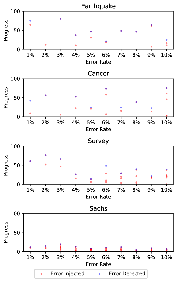
Figure 4. ED-Check on four datasets.

Table 2. Sensitivity of error detection.

Dataset	Earthquake	Cancer	Survey	Sachs
Sensitivity	15.1%	25.0%	21.5%	8.0%

We present the error detection results in Fig. 4. Red dots represent the normalized position (by the total number of CI tests) where errors are injected, and blue dots indicate where ED-Check detects them. Overlapping red and blue dots indicate immediate error detection upon injection. We observe that ED-Check successfully detects errors in most cases (38 out of 40), excluding “2%” of Earthquake and “3%” of Cancer. Error detection sensitivity is also quantified in Table 2, calculated by subtracting the normalized progress of the first error detection from that of the error injection. For instance, sensitivity in Fig. 4 is determined by the distance between the first red and blue dot in each plot. Overall, ED-Check  exhibits high sensitivity to errors, with six detected immediately and 25 within 15% of the total CI tests.

Failure Case Analysis. We also inspected the two failure cases in Fig. 4. In both cases, errors are injected into a marginal CI statement. As aforementioned in Sec. 4.2.1, marginal CI statements themselves would not violate Pearl’s axioms. If there is no other high-order CI statements that trigger the inconsistency, ED-Check cannot detect the error by design. Unfortunately, the injected errors do not violate any high-order CI statements. Indeed, despite the error, we find that the learned causal skeleton is identical to the ground truth. Hence, we presume these errors may be too subtle to be detected.

Answer to RQ1: When benchmarked using common causal discovery datasets with sufficient complexity, ED-Check uncovers erroneous CI statements with high accuracy and also high sensitivity.

6.3. Effectiveness of P-Check

In this evaluation, we employ the perfect CI oracle as well as two distinct CI test schemes to evaluate the performance of P-Check in reducing the number of CI tests produced by the PC algorithm. The first CI test scheme is the well-established $\chi^{2}$ test (Pearson, 1900), a statistical hypothesis test that assesses the independence of two categorical variables. This test is widely used in causal discovery and often serves as the default CI test scheme in many causal discovery tools. Hence, the result of the $\chi^{2}$ test provides a baseline for assessing the effectiveness of P-Check in realistic settings. The second scheme is the differentially private Kendall’s $\tau$ test (Wang et al., 2020), which is designed to protect the privacy of the dataset by introducing controlled noise into the test statistics. This test is particularly useful for evaluating the performance of P-Check in privacy-sensitive applications, where the traditional $\chi^{2}$ test may not be suitable due to the disclosure risks associated with its non-private nature. By incorporating these two CI test schemes, we aim to demonstrate P-Check’s applicability in handling diverse CI test schemes.

Table 3. Performance with the perfect CI Oracle.

Dataset	#CI Tests w/o P-Check	#CI Tests w/ P-Check
Earthquake	56	22 (-60.7%)
Cancer	57	22 (-61.4%)
Survey	115	51 (-55.7%)
Sachs	1258	818 (-35.0%)

P-Check with Perfect CI Oracle. We present the results of our experiments with the perfect CI oracle on four datasets in Table 3. We compared the number of CI tests generated by the PC algorithm with and without P-Check using a perfect CI oracle. The results are shown in Table 3, where we observe that P-Check is highly successful in decreasing the number of required CI tests across all datasets. Specifically, for datasets with five or six variables, namely Earthquake, Cancer, and Survey, we achieve a reduction ranging from 55.7% to 60.7%. Even on the challenging Sachs dataset with 11 variables, where the UF to a CI statement can have up to $2^{33}$ states, P-Check demonstrates a significant reduction of 35.0%.

As discussed in Sec. 4.2.4, the CIR problem solving is sound and complete, which means that P-Check does not yield any erroneous CI statements. Indeed, we observe that the learned causal skeleton is identical to the ground-truth skeleton when using the perfect CI oracle, with no additional errors introduced.

Table 4. Effectiveness of P-Check in terms of #CI Test, Structural Hamming Distance (SHD) and privacy budget ($\epsilon$). “ER-$n$” denotes the synthetic dataset with $n$ variables and “ER-15” denotes the largest synthetic dataset with 15 variables.

Metric	Earthquake	Cancer	Survey	Sachs	ER-5	ER-10	ER-15
DP Kendall’s $\tau$ Test (averaged on ten runs)
#CI Test	37.7$\to$16.2	16.8$\to$10.7	45.9$\to$16.1	264.3$\to$156.2	13.3$\to$10.0	86.7$\to$67.0	190.0$\to$153.3
SHD	2.7$\to$2.6	2.8$\to$2.6	2.5$\to$0.7	13.9$\to$13.0	1.7$\to$2.0	7.3$\to$7.0	20.3$\to$18.7
$\epsilon$	54.6$\to$34.3	38.3$\to$32.1	60.2$\to$40.8	277.9$\to$208.5	35.2$\to$29.9	141.7$\to$118.8	280.6$\to$238.4
$\chi^{2}$ Test
#CI Test	56$\to$22	75$\to$36	69$\to$30	1277$\to$816	15$\to$11	208$\to$136	610$\to$475
SHD	0$\to$0	2$\to$2	0$\to$0	1$\to$1	0$\to$0	1$\to$1	4$\to$4

P-Check with Imperfect CI Tests. The efficacy of P-Check is validated on two imperfect CI test schemes: DP Kendall’s $\tau$ and $\chi^{2}$ Tests. The results are in Table 4. SHD represents the “edit distance” from the learned graph to the ground truth; a lower value is preferable. Total privacy for executing DP Kendall’s $\tau$ tests is denoted by $\epsilon$; a lower value is preferable. Owing to the probabilistic character of the DP-enforced algorithm, the DP Kendall’s $\tau$ Test is repeated ten times and the average outcome is reported. P-Check efficiently reduces the necessary CI tests count while maintaining competitive SHD accuracy across all data sets. On average, P-Check results in a reduction of 38.0% and 41.2% in CI tests using DP Kendall’s $\tau$ and $\chi^{2}$ Tests respectively, across all datasets. Moreover, there is an observable slight increase in accuracy (lower SHD) under the DP setting compared to Priv-PC (Wang et al., 2020). This is presumably because P-Check sidesteps the high number of CI tests that are typically incorrect. In addition, P-Check offers superior privacy protection, as indicated by a substantially lower $\epsilon$.

Answer to RQ2: P-Check effectively prunes excessive CI tests in both perfect and imperfect CI test schemes. It reduces CI tests by 35.0% to 60.7% with the perfect CI oracle and retains accuracy while providing better privacy protection in imperfect CI tests.

6.4. Ablation Study

In RQ3, we aim to evaluate the effectiveness of our proposed optimizations and explore their impact on the overall performance. Recall that there are three optimizations in CICheck, namely $\mathcal{O}_{1}$ MA, $\mathcal{O}_{2}$ GR, and $\mathcal{O}_{3}$ CD. In particular, $\mathcal{O}_{1}$ is used to prove consistency while $\mathcal{O}_{2}$ and $\mathcal{O}_{3}$ are used to refute consistency. Thus, given their different purposes, we employ distinct evaluation strategies for $\mathcal{O}_{1}$ and the other two optimizations. We measure $\mathcal{O}_{1}$’s effectiveness through the entire lifecycle of the causal discovery. On the other hand, $\mathcal{O}_{2},\mathcal{O}_{3}$ are particularly effective when dealing with inconsistent CI statements. In ED-Check, there is at most one inconsistent case (since we abort execution once an inconsistency is detected). Hence, we measure the effectiveness of $\mathcal{O}_{2},\mathcal{O}_{3}$ on multiple instances of the CIR problem. Below, we present the impact of them.

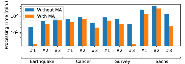
Figure 5. Comparison of processing time (each bar represents an individual run).

Effectiveness of $\mathcal{O}_{1}$ MA. The effectiveness of $\mathcal{O}_{1}$ is first evaluated through a comparison of processing times between ED-Check with and without $\mathcal{O}_{1}$. Our experiment involves injecting 5% errors into CI statements. The random seed remains fixed per comparison group. Each dataset undergoes three comparative groupings. As shown in Fig. 5, $\mathcal{O}_{1}$ notably reduces the time. Specifically, CICheck immediately flags the error in the initial non-marginal CI statements in the first case of Earthquake and the third case of Survey. As a result, in such situations, $\mathcal{O}_{1}$ makes CICheck almost effortless. On average, $\mathcal{O}_{1}$ achieves a speedup of 48.9% ($\pm$ 25.7%) across all datasets, with a maximum reduction of 93.8%. Our interpretation is that $\mathcal{O}_{1}$ effectively accelerates CICheck without compromising accuracy.

Effectiveness of $\mathcal{O}_{2}$ GR and $\mathcal{O}_{3}$ CD. We then evaluate the effectiveness of $\mathcal{O}_{2}$ and $\mathcal{O}_{3}$. To fully unleash the power of $\mathcal{O}_{2}$ and $\mathcal{O}_{3}$, we use the Sachs dataset, which is the largest dataset in our experiments. On the remaining datasets, we observe similar performance boosts from $\mathcal{O}_{2}$ and $\mathcal{O}_{3}$ (see Sec. H of Supp. Material). In particular, we collect a total of 1,258 CI statements from the error-free execution on the Sachs dataset. Then, we randomly flip some CI statements (as well as their symmetric counterparts) to create a knowledge base such that each knowledge base contains roughly 5% erroneous CI statements. Hence, we obtain one instance of the CIR problem with erroneous CI statements that may be inconsistent with the Pearl’s axioms. We check whether the inconsistent knowledge bases can be refuted by $\mathcal{O}_{2}$ or $\mathcal{O}_{3}$, respectively. We also measure the processing time. We repeat the experiments 100 times and report the average running time and the overall refutability.

Table 5. Effectiveness of $\mathcal{O}_{2}$ GR and $\mathcal{O}_{3}$ CD. “avg.”, “mdn.” and “max.” denotes the mean, median and maximum.

	Refutability	Processing time (avg. / mdn. / max.)
$\mathcal{O}_{2}$	91/100	0.6 / 0.6 / 0.7
$\mathcal{O}_{3}$ w/o Full	53/100	14.3 / 10.9 / 25.8
$\mathcal{O}_{3}$	100/100	25.6 / 5.3 / 58.2
$\mathcal{O}_{2}$ + $\mathcal{O}_{3}$	100/100	2.4 / 0.6 / 53.8

As shown in Table 5, in a series of 100 experiments, $\mathcal{O}_{2}$ has an efficacy of refuting 91% of the inconsistent knowledge bases, and $\mathcal{O}_{3}$ — when combined with full constraint solving — manages to refute 100% of the inconsistencies, while the decomposed constraints alone can only address 53% of the errors. When both $\mathcal{O}_{2}$ and $\mathcal{O}_{3}$ are applied together, they detect all errors, enhancing their collective effectiveness. We notice that the median processing time of $\mathcal{O}_{2}$ is significantly lower (0.6 seconds) as compared to that of using decomposed constraints alone, which requires 10.9 seconds, and extends to 5.3 seconds when used alongside the full constraint, marking $\mathcal{O}_{2}$ as both efficient and highly sensitive towards inconsistent knowledge bases. Besides, we observe notable variations in the mean, median, and maximum processing time for $\mathcal{O}_{2}$ + $\mathcal{O}_{3}$. We interpret the result as follows. The processing time primarily clusters around two scenarios; the majority approximating 0.6 seconds (case 1), with the remainder around 53.8 seconds (case 2). The first case corresponds to situations where $\mathcal{O}_{2}$, a lightweight scheme, swiftly refutes consistency. The latter case occurs when an SMT solver is involved and requires more time to resolve the CIR problem.

On the other hand, $\mathcal{O}_{3}$ provides a comprehensive overview of the CIR problem and detects all errors, serving as an effective complement to $\mathcal{O}_{2}$ by refuting additional inconsistent knowledge bases. From another perspective, $\mathcal{O}_{2}$ significantly reduces the costs associated with $\mathcal{O}_{3}$ by detecting numerous errors early on. Simultaneous adoption of $\mathcal{O}_{2}$ and $\mathcal{O}_{3}$ trims down the processing time to 2.3 seconds, yielding a solution that is more accurate than using $\mathcal{O}_{2}$ alone, and remarkably faster than just utilizing $\mathcal{O}_{3}$.

Answer to RQ3: All three optimizations significantly contribute to the performance of CICheck. Specifically, $\mathcal{O}_{1}$ reduces the processing time by a significant margin, while $\mathcal{O}_{2}$ and $\mathcal{O}_{3}$ are effective and efficient in detecting and refuting inconsistent knowledge bases. The synergistic effect of these optimizations makes CICheck practical.

6.5. Discussion

Potential Impact in Software Engineering. We articulate the potential impact of our work in the SE community from two perspectives. ➊ Causal Inference in SE: Causal inference is gaining traction as an important methodology within SE (Fariha et al., 2020; Dubslaff et al., 2022; Johnson et al., 2020; Hsiao et al., 2017; Ji et al., 2022; Siebert, 2023; Ji et al., 2022, 2023a; Sun et al., 2022; Zhang and Sun, 2022; Ji et al., 2023b). The prosperous use of causal inference algorithms makes CICheck an important contribution that uniquely addresses both privacy and reliability concerns. This positions CICheck as a useful tool in the fast-evolving SE landscape. ➋ Methodological Integration: CICheck  delivers a novel adoption of classical SE techniques, e.g., formal verification and constraint solving. This synergy, to a degree, enables CICheck to expand the existing formal method realm into a novel and crucial domain — causal discovery.

Scalability. Automated reasoning is often costly, and the scalability of our framework is on par with that of other SMT/SAT-based causal discovery algorithms (Zhalama et al., 2019; Hyttinen et al., 2013) (e.g., causal graph with roughly a dozen of nodes). Causal discovery algorithms often struggle with high-dimensional data, which is why ED-Check focuses on datasets with moderate complexity; de facto causal discovery algorithms are anticipated to behave reliably and perform well over these datasets. In terms of P-Check, existing constraint-based privacy-preserving causal discovery algorithms, such as EM-PC (Xu et al., 2017), share a similar scalability regime. However, Priv-PC (Wang et al., 2020) shows a better scalability which handles larger datasets like ALARM and INSURANCE (bnl, 2023). Notably, CICheck has a unique role compared to these algorithms, potentially enhancing their privacy-preserving abilities, evidenced by P-Check’s improvement on Priv-PC (Sec. 6.3). Looking ahead, we plan to boost CICheck with advanced SMT solvers like CVC5 (Barbosa et al., 2022).

Extension to Other Causal Discovery Algorithms. Since CICheck does not rely on any execution information about the underlying algorithms, it is agnostic to specific causal discovery implementations. Hence, our framework can be smoothly extended to other causal discovery algorithms by replacing the employed standard CI test algorithm with the one hardened by CICheck. For instance, we envision that CICheck can be applied to enhance the federated causal discovery algorithm (Wang et al., 2023) to reduce privacy leakage. However, CICheck is not applicable to enhance causal discovery algorithms that do not use CI tests (e.g., functional causal models (Peters et al., 2017; Ma et al., 2022b) or score-based methods (Tsamardinos et al., 2006)) or leverage quantitative information beyond qualitative CI relations (e.g., p-values (Ma et al., 2022a; Ding et al., 2020)).

Threats to Validity. Our framework is implemented using standard tool chains and the experiments are conducted with widely-used datasets and CI test algorithms. Nonetheless, potential threats to the validity of our results persist. Firstly, our framework’s performance may be contingent on the choice of CI test algorithms and datasets. To alleviate this risk, we have tested our framework with multiple CI test algorithms and datasets. Secondly, our framework’s scalability may face limitations when employed on large-scale datasets or complex causal structures. To address this, we propose several optimizations to improve efficiency. Thirdly, the generalizability of our results may be influenced by the specific implementation choices within our framework. To mitigate this threat, we conducted experiments on several datasets and CI test algorithms repetitively to ensure the robustness of our results. Besides, using random error injection in Sec. 6.2 may not perfectly simulate real-world cases. In this regard, our findings’ applicability might be limited. Integrating CICheck with causal learning tools (cau, 2023) would be a beneficial way to confirm the validity. As mentioned in Sec. 5, it is theoretically conceivable that multiple incorrect facts could weaken the effectiveness of ED-Check. While we deem this scenario rare due to the tight integrity constraints by Pearl’s axioms and empirically show its unlikelihood in practice (Sec. 6.3 and Sec. F of Supp. Material), we acknowledge it as a threat to validity. Statistical errors could cause P-Check to malfunction because of inconsistent knowledge bases or faulty reasoning (i.e., deriving an incorrect CI from another wrong CI). We address inconsistencies in the knowledge bases by employing a backtracking mechanism to restore previous states (Sec. 5). We demonstrate empirically that P-Check does not compromise causal discovery accuracy, proving its resilience to statistical errors (Sec. 6.3).

7. Related Work

We have reviewed the related works in causal discovery in Sec. 2. In this section, we discuss the related work in formal methods for CI implication and causal inference in software engineering.

CI Implication. Some studies aim to infer CI statements through implications. Instead of using Pearl’s axioms, they attempt to characterize specific classes of distribution and infer CI statements using algebraic or geometric reasoning methods (Bouckaert and Studenỳ, 2007; Bouckaert et al., 2010; Tanaka et al., 2015; Niepert et al., 2013). It is worth noting that these approaches are not applicable in our context. Firstly, they cannot reason over conditional dependence — a prevalent and essential inference case in our scenario. Secondly, they often exhibit limited scalability and narrow applicability (e.g., the racing-based method (Bouckaert and Studenỳ, 2007) can only handle five variables).

Causality in Software Engineering. Causality has become an increasingly prevalent technique in software engineering (Fariha et al., 2020; Dubslaff et al., 2022; Johnson et al., 2020; Hsiao et al., 2017; Ji et al., 2022; Siebert, 2023; Ji et al., 2022, 2023a). These tools typically concentrate on examining the effects of program inputs or configurations on software behavior, such as execution time or crashes. Moreover, due to its inherent interpretability, causality analysis is extensively utilized in the testing and repair of machine learning models (Sun et al., 2022; Zhang and Sun, 2022; Ji et al., 2023b).

8. Conclusion

We have presented CICheck, a novel runtime verification tool for causal discovery algorithms that addresses both reliability and privacy concerns in reliability-critical and privacy-critical usage scenarios in a unified approach. Experiments on various synthetic and real-world datasets show that CICheck enhances both reliability-critical and privacy-critical scenarios with a moderate overhead. We envision our work can inspire more research on the extension of SE methodology to the domain of causal inference.

Appendix A Preliminaries

d-separation. In a DAG, two sets of nodes $\bm{X}$ and $\bm{Y}$ are said to be d-separated by $\bm{Z}$ if and only if there is no active undirected path between $\bm{X}$ and $\bm{Y}$ given $\bm{Z}$. An undirected path between $X\in\bm{X}$ and $Y\in\bm{Y}$ is active relative to $\bm{Z}$ if (i) every non-collider on $U$ is not a member of $\bm{Z}$ and (ii) every collider on $U$ has a descendant in $\bm{Z}$. Here, $U$ is said to be a collider on the path if the edges connected $U$ form the structure of $\to U\leftarrow$. Intuitively, the $d$-separation relation can be seen as a graphical analogy of CI in data. In other words, all paths being deactivated by $\bm{Z}$ indicates that the causal relation between $\bm{X}$ and $\bm{Y}$ is blocked by $\bm{Z}$.

Faithful Bayesian Network. A Bayesian network is said to be faithful if and only if it satisfies the following two conditions: (i) the Markov condition and (ii) the faithfulness condition. The Markov condition states that every node is independent of its non-descendants given its parents. The faithfulness condition states that every CI in the distribution is entailed by the DAG. In other words, the faithfulness condition states that the DAG is minimal in the sense that removing any edge from the DAG will result in a distribution that does not entail the CI.

Appendix B Encoding of Pearl’s Axioms

Symmetry.

(23) $$\forall BV_{\bm{X}},BV_{\bm{Y}},BV_{\bm{Z}}\in\{0,1\}^{|\bm{V}|}$$

$$\texttt{CI}(BV_{\bm{X}},BV_{\bm{Y}},BV_{\bm{Z}})=\texttt{CI}(BV_{\bm{Y}},BV_{\bm{X}},BV_{\bm{Z}})$$

Decomposition.

(24) $$\forall BV_{\bm{X}},BV_{\bm{Y}},BV_{\bm{Z}},BV_{\bm{W}}\in\{0,1\}^{|\bm{V}|}$$

$$\texttt{CI}(BV_{\bm{X}},BV_{\bm{Y}}|BV_{\bm{W}},BV_{\bm{Z}})=\texttt{01}\implies\texttt{CI}(BV_{\bm{X}},BV_{\bm{Y}},BV_{\bm{Z}})=\texttt{01}$$

$$\texttt{CI}(BV_{\bm{X}},BV_{\bm{Y}}|BV_{\bm{W}},BV_{\bm{Z}})=\texttt{01}\implies\texttt{CI}(BV_{\bm{X}},BV_{\bm{W}},BV_{\bm{Z}})=\texttt{01}$$

Weak Union.

(25) $$\forall BV_{\bm{X}},BV_{\bm{Y}},BV_{\bm{Z}},BV_{\bm{W}}\in\{0,1\}^{|\bm{V}|}$$

$$\texttt{CI}(BV_{\bm{X}},BV_{\bm{Y}}|BV_{\bm{W}},BV_{\bm{Z}})=\texttt{01}\implies\texttt{CI}(BV_{\bm{X}},BV_{\bm{Y}},BV_{\bm{Z}}|BV_{\bm{W}})=\texttt{01}$$

Contraction.

(26) $$\forall BV_{\bm{X}},BV_{\bm{Y}},BV_{\bm{Z}},BV_{\bm{W}}\in\{0,1\}^{|\bm{V}|}$$

$$\texttt{CI}(BV_{\bm{X}},BV_{\bm{Y}},BV_{\bm{Z}})=\texttt{01}\land\texttt{CI}(BV_{\bm{X}},BV_{\bm{W}},BV_{\bm{Y}}|BV_{\bm{Z}})=\texttt{01}\implies\texttt{CI}(BV_{\bm{X}},BV_{\bm{Y}}|BV_{\bm{W}},BV_{\bm{Z}})=\texttt{01}$$

Intersection.

(27) $$\forall BV_{\bm{X}},BV_{\bm{Y}},BV_{\bm{Z}},BV_{\bm{W}}\in\{0,1\}^{|\bm{V}|}$$

$$\texttt{CI}(BV_{\bm{X}},BV_{\bm{Y}},BV_{\bm{Z}}|BV_{\bm{W}})=\texttt{01}\land\texttt{CI}(BV_{\bm{X}},BV_{\bm{W}},BV_{\bm{Y}}|BV_{\bm{Z}})=\texttt{01}\implies\texttt{CI}(BV_{\bm{X}},BV_{\bm{Y}}|BV_{\bm{W}},BV_{\bm{Z}})=\texttt{01}$$

Composition.

(28) $$\forall BV_{\bm{X}},BV_{\bm{Y}},BV_{\bm{Z}},BV_{\bm{W}}\in\{0,1\}^{|\bm{V}|}$$

$$\texttt{CI}(BV_{\bm{X}},BV_{\bm{Y}},BV_{\bm{Z}})=\texttt{01}\land\texttt{CI}(BV_{\bm{X}},BV_{\bm{W}},BV_{\bm{Z}})=\texttt{01}\implies\texttt{CI}(BV_{\bm{X}},BV_{\bm{Y}}|BV_{\bm{W}},BV_{\bm{Z}})=\texttt{01}$$

Weak Transitivity.

(29) $$\forall BV_{\bm{X}},BV_{\bm{Y}},BV_{\bm{Z}},BV_{\bm{W}},BV_{U}\in\{0,1\}^{|\bm{V}|}$$

$$|BV_{U}|=1\land\texttt{CI}(BV_{\bm{X}},BV_{\bm{Y}},BV_{\bm{Z}})=\texttt{01}\land\texttt{CI}(BV_{\bm{X}},BV_{\bm{W}},BV_{\bm{Z}}|BV_{U})=\texttt{01}\implies\texttt{CI}(BV_{U},BV_{\bm{Y}},BV_{\bm{Z}})=\texttt{01}$$

$$|BV_{U}|=1\land\texttt{CI}(BV_{\bm{X}},BV_{\bm{Y}},BV_{\bm{Z}})=\texttt{01}\land\texttt{CI}(BV_{\bm{X}},BV_{\bm{W}},BV_{\bm{Z}}|BV_{U})=\texttt{01}\implies\texttt{CI}(BV_{\bm{X}},BV_{U},BV_{\bm{Z}})=\texttt{01}$$

Chordality.

(30) $$\forall BV_{{X}},BV_{{Y}},BV_{{Z}},BV_{{W}}\in\{0,1\}^{|\bm{V}|}$$

$$|BV_{X}|=1\land|BV_{Y}|=1\land|BV_{Z}|=1\land|BV_{W}|=1\land\texttt{CI}(BV_{{X}},BV_{{Y}},BV_{{Z}}|BV_{W})=\texttt{01}\land\texttt{CI}(BV_{Z},BV_{{W}},BV_{{X}}|BV_{Y})=\texttt{01}$$

$$\implies\texttt{CI}(BV_{X},BV_{{Y}},BV_{{Z}})=\texttt{01}$$

$$|BV_{X}|=1\land|BV_{Y}|=1\land|BV_{Z}|=1\land|BV_{W}|=1\land\texttt{CI}(BV_{{X}},BV_{{Y}},BV_{{Z}}|BV_{W})=\texttt{01}\land\texttt{CI}(BV_{Z},BV_{{W}},BV_{{X}}|BV_{Y})=\texttt{01}$$

$$\implies\texttt{CI}(BV_{X},BV_{{Y}},BV_{{W}})=\texttt{01}$$

Appendix C PC Algorithm

1 Function Skeleton-Learning($X_{1},\cdots,X_{d}$):

2       initialize a complete undirected graph $Q$ with $d$ nodes;

3       $n\leftarrow 0$;

4      

5      repeat

6            

7            repeat

8                   select an ordered pair of adjacent nodes $X,Y$ such that $\textit{Neighbor}(X)\setminus\{Y\}$ has cardinality $\geq n$, and a subset $\bm{S}\subseteq\textit{Neighbor}(X)\setminus\{Y\}$ of cardinality $n$, and, if $X\Perp Y\mid S$, delete the edge between $X$ and $Y$ from $Q$, and record $\bm{S}$ in $\textit{Sepset}(X,Y)$ and $\textit{Sepset}(Y,X)$;

9            until all ordered pairs of adjacent nodes $X$ and $Y$ such that $\textit{Neighbor}(X)\setminus\{Y\}$ has cardinality $\geq n$ and all subsets $\bm{S}$ in $\textit{Neighbor}(X)\setminus\{Y\}$ have been tested for d-separation;

10            $n\leftarrow n+1$;

11            

12      until for each ordered pair of adjacent nodes $X,Y$, $\textit{Neighbor}(X)\setminus\{Y\}$ has less than $n$ neighbors;

13      return $Q$

14

15

16Function PC($X_{1},\cdots,X_{d}$):

       /* skeleton learning */

17       $G\leftarrow\textnormal{{Skeleton-Learning}}(X_{1},\cdots,X_{d})$;

       /* orientation */

18       foreach unshielded triple $(X-Z-Y)$ in $G$ do

19             if $\forall X\Perp Y\mid G,Z\notin G$ then

20                   orient $(X-Z-Y)$ as $(X\to Z\leftarrow Y)$;

21            

22       end foreach

      /* apply Meek’s rule (Meek, 1995) to orient the remaining edges */

23       repeat

24             foreach $(X\to Z-Y)$ do orient as $(X\to Z\leftarrow Y)$;

25             foreach $(X\to Z\to Y)$ and $(X-Y)$ do orient as $(X\to Y)$;

26             foreach $(X-Y)$, $(X-Z)$, $(X-W)$, $(Z\to Y)$, $(W\to Y)$ and $Z,W$ is nonadjacent do orient as $(X\to Y)$;

27            

28      until no more edgs can be oriented;

29      return $G$

30

Algorithm 2 PC Algorithm

We present the workflow of the PC algorithm (Spirtes et al., 2000) in Alg. 2. In the first step (lines 1–10; line 12), edge adjacency is confirmed if there is no conditional independence between two variables (line 6). In the second step (lines 13–21), a set of orientation rules are applied based on conditional independence and graphical criteria.

Appendix D Preparation of Synthetic Datasets

Following the setup in EM-PC (Xu et al., 2017), we sample random graphs from the Erdős–Rényi graphical model (Erdős et al., 1960) with different node size. Then, we sample the corresponding joint distribution from the Dirichlet-multinomial distribution (i.e., the family distributions of our probability distributions). We use the default parameters from EM-PC (Xu et al., 2017) to generate the synthetic datasets.

Appendix E Complexity of Benchmark Problems

Table 6. Statistics of SMT Problems (avg. on ten runs). #quant-instantiations indicates the number of instantiated quantifiers.

Dataset	Memory Usage (MB)	Solving Time (sec.)	#quant-instantiations
Earthquake	20	0.3	192.0
Cancer	21	0.9	257.9
Survey	22	0.8	337.2
Sachs	96	33.9	2728.4

Number of SMT Constraints. Our encoding scheme posits a linear relationship between SMT constraints and CI statements. Recall that Pearl’s axioms are enforced into a constant number of first-order constraints and each CI statement is encoded into a propositional equality constraint on the uninterpreted function CI. Therefore, with $n$ CI statements, we have $n$ CI equality constraints alongside $8$ first-order constraints, totalling $n+8$ SMT Constraints. Accordingly, the max number of SMT constraints per dataset in Table 1 are 64, 65, 123 and 1266, respectively. We consider such constraint sizes as moderate and can be smoothly handled by our technique.

Statistics of SMT Problem Instances. In addition to the number of SMT constraints, we present additional key metrics for each dataset’s largest SMT problem instance (the same instance in Sec. 6.4) in Table 6. The sizes of these problems are generally considered moderate. On the other hand, for datasets like Earthquake, Cancer, and Survey, the resolution time does not correlate highly with the size of CI statements. This might be due to their relatively smaller sizes, making them more responsive to external factors such as the particular optimizations employed by the SMT solver.

Appendix F Detectability of ED-Check

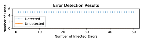
Figure 6. Detectability of ED-Check on the Survey dataset under different error numbers. The best detectability is achieved when the “Number of Cases” for “Detected” is 5. That is, ED-Check flags all erroneous cases.

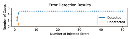
Figure 7. Detectability of ED-Check on the Sachs dataset under different error numbers. The best detectability is achieved when the “Number of Cases” for “Detected” is 5. That is, ED-Check flags all erroneous cases.

We study the detectability of ED-Check on the Survey and Sachs datasets (representing two largest datasets in our experiments from the bnlearn repository). In particular, we randomly inject one to fifty errors into the 1,258 CI statements. We then run ED-Check on the corrupted CI statements and record the number of errors detected. We repeat this process five times with different random seeds. The results are presented in Fig. 6 and Fig. 7. We observe that ED-Check can detect nearly all errors. Notably, detection failures occur only in three instances on the Sachs dataset (the largest dataset), when the error count is one (corresponding to an error rate of $0.08\%$). Considering these encouraging results, it is believed that ED-Check offers highly practical detectability, even for very subtle errors.

Appendix G End-to-end Effectiveness of $\mathcal{O}_{2},\mathcal{O}_{3}$

Table 7. End-to-end processing time of $\mathcal{O}_{2}$ GR and $\mathcal{O}_{3}$ CD under when using P-Check.

	Earthquake	Cancer	Survey	Sachs
$\mathcal{O}_{1}$	0:22:53	0:22:47	0:50:16	10:21:42
$\mathcal{O}_{1}$ + $\mathcal{O}_{2}$	0:21:52	0:21:49	0:46:14	10:16:00
$\mathcal{O}_{1}$ + $\mathcal{O}_{3}$	0:09:38	0:09:51	0:27:29	7:15:01
Full Optimization	0:09:24	0:07:35	0:25:21	7:03:15

We report the end-to-end processing time of P-Check under different optimization levels in Table 7. Since the process of P-Check does not involve any randomness, we only run each experiment once. Overall, we view each optimization as effective, as it reasonably reduces the processing time. In particular, $\mathcal{O}_{3}$ proves to be the most impactful optimization by reducing the average processing time by 47.5%. The effectiveness of $\mathcal{O}_{3}$ is attributed to its lightweight constraint-solving scheme that allows for quick disproval of the global consistency in CI statements and an “early stop” to the overall constraint-solving procedure. On the other hand, we observe $\mathcal{O}_{2}$ is less effective than $\mathcal{O}_{3}$. Despite this, $\mathcal{O}_{2}$ still contributes to an encouraging 4.4% average increase in speed. Overall, the full optimization scheme (i.e., $\mathcal{O}_{1}+\mathcal{O}_{2}+\mathcal{O}_{3}$) delivers 51.8% average speedup over the baseline ($\mathcal{O}_{1}$ only).

Appendix H Extended Experiments for RQ3

Table 8. Effectiveness of $\mathcal{O}_{2}$ GR and $\mathcal{O}_{3}$ CD on Earthquake.

	Refutability	Avg. processing time (sec.)
$\mathcal{O}_{2}$	63/100	0.01
$\mathcal{O}_{3}$	100/100	0.9
$\mathcal{O}_{2}$ + $\mathcal{O}_{3}$	100/100	0.1

Table 9. Effectiveness of $\mathcal{O}_{2}$ GR and $\mathcal{O}_{3}$ CD on Cancer.

	Refutability	Avg. processing time (sec.)
$\mathcal{O}_{2}$	63/100	0.01
$\mathcal{O}_{3}$	100/100	0.7
$\mathcal{O}_{2}$ + $\mathcal{O}_{3}$	100/100	0.3

Table 10. Effectiveness of $\mathcal{O}_{2}$ GR and $\mathcal{O}_{3}$ CD on Survey.

	Refutability	Avg. processing time (sec.)
$\mathcal{O}_{2}$	93/100	0.03
$\mathcal{O}_{3}$	100/100	0.9
$\mathcal{O}_{2}$ + $\mathcal{O}_{3}$	100/100	0.1