Iterative Phase Retrieval Algorithms for Scanning Transmission Electron Microscopy

^† These authors contributed equally to this work.

Scanning transmission electron microscopy (STEM) has been extensively used for imaging complex materials down to atomic resolution. The most commonly employed STEM imaging modality of annular dark field produces easily-interpretable contrast, but is dose-inefficient and produces little to no contrast for light elements and weakly-scattering samples. An alternative is to use phase contrast STEM imaging, enabled by high speed detectors able to record full images of a diffracted STEM probe over a grid of scan positions. Phase contrast imaging in STEM is highly dose-efficient, able to measure the structure of beam-sensitive materials and even biological samples. Here, we comprehensively describe the theoretical background, algorithmic implementation details, and perform both simulated and experimental tests for three iterative phase retrieval STEM methods: focused-probe differential phase contrast, defocused-probe parallax imaging, and a generalized ptychographic gradient descent method implemented in two and three dimensions. We discuss the strengths and weaknesses of each of these approaches using a consistent framework to allow for easier comparison. This presentation of STEM phase retrieval methods will make these methods more approachable, reproducible and more readily adoptable for many classes of samples.

1 Introduction

The “phase problem” – describing the loss of phase information of complex-valued scattering objects during intensity measurements – is a well-known challenge in many imaging and diffraction fields including crystallography, astronomy, and microscopy [1]. Phase contrast imaging techniques, such as Zernike phase contrast microscopy (PCM) [2, 3] and differential phase contrast (DPC) [4], attempt to solve this by converting phase variations in the object plane into intensity variations in the imaging plane. Conversely, phase retrieval techniques attempt to recover the missing phase information by leveraging redundant information in the dataset and prior information such as finite support and positivity in the form of projections and regularization constraints [1, 5]. Such techniques often involve iterative reconstruction algorithms and are thus are also referred to as computational or lensless imaging techniques  [6].

Phase retrieval techniques offer particular promise in (scanning) transmission electron microscopy (S/TEM) as they enable the dose-efficient observation of otherwise imperceptible signals from weakly-scattering and dose-sensitive samples [7, 8, 9]. While early phase retrieval microscopy techniques such as coherent diffractive imaging (CDI) used a parallel-beam illumination and a single diffraction measurement [10], significant advantages can be conferred by the diversity of information obtained in scanning a converged-beam illumination across the sample and collecting diffraction intensities at each probe position. In electron microscopy this imaging mode is often referred to as 4D scanning transmission electron microscopy (4D-STEM) (fig. 1a), due to the dimensionality of the resulting dataset having two (real-space) scan dimensions and two (reciprocal-space) diffraction dimensions [11].

Part of the rapid development that phase retrieval in electron microscopy has experienced in the last decade is due to the fact that many of the guiding principles translate well across similar techniques developed for longer-wavelength illumination such as x-ray and light microscopy, and more broadly from the field of non-convex optimization [12, 13, 14]. However, various nuances of the scattering physics, 4D-STEM geometry, and electron optics suggest that existing algorithms can benefit from the development of domain-specific efficient regularization constraints.

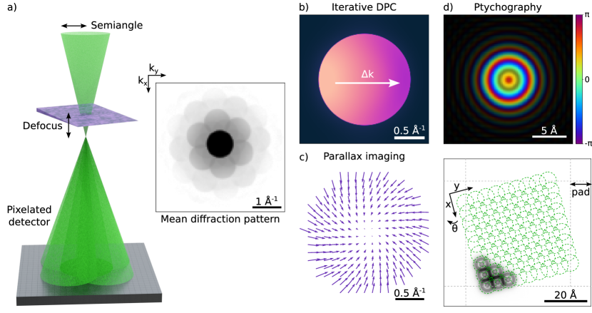
Figure 1: a) 4D-STEM geometry schematic. A converged probe is scanned across a sample, with diffraction intensities being recorded on a pixelated detector. b) Center of mass shift schematic used in DPC, resulting from long-range fields. c) Cross-correlation vector field for virtual bright field alignment used during parallax reconstruction. d) Probe and object field-of-view parameters relevant for ptychography.

Here, we present a consistent framework for various phase-retrieval algorithm implementations designed for 4D-STEM datasets, with a particular emphasis on robustness against common experimental artifacts, available in the open-source 4D-STEM analysis software package py4DSTEM [15]. In particular, we highlight three classes of iterative phase-retrieval techniques: i) iterative DPC (fig. 1b), ii) parallax imaging (fig. 1c), and iii) a suite of ptychographic reconstructions in two- and three-dimensions (fig. 1d). The implementations discussed below include a combination of previously published algorithms as well as original research, and we highlight our contributions to the field throughout the text.

The manuscript is structured as-follows: First, in sections 2 and 3 we introduce the theory for the iterative DPC and parallax phase-retrieval techniques, and demonstrate their utility on simulated datasets for focused-probe and defocused-probe geometries respectively. In addition to the reconstructed phases, these techniques provide valuable tools to estimate necessary preprocessing parameters for ptychographic reconstructions, namely the relative rotation and alignment of the diffraction intensities coordinate system with respect to the scan coordinate system and low-order aberrations such as defocus. We then introduce the theory for single-slice ptychography in section 4 and discuss common preprocessing parameters and their impact on the resulting reconstruction. Next, we start relaxing the multiplicative-assumption of single-slice ptychography by modifying the forward and adjoint operators to include partial-coherence (section 5), depth-sectioning (section 6), and three-dimensional scattering (section 7). Finally, we discuss domain-specific regularization constraints for the illuminating probe and reconstructed object in section 8, before highlighting the performance of the algorithms on experimental datasets in section 9.

2 Iterative Differential Phase Contrast

When an electron beam interacts with a sample’s electrostatic potential the center of mass (CoM) of the incident beam shifts, and the nature of the shift is related to the probe and feature size (fig. 2a) [16]. Atomic-scale features tend to lead to redistribution of signal within the bright field disk, while long-range (slowly-varying) fields cause rigid shifts of the entire bright field disk. Early techniques captured this change in center of mass through segmented detectors, using a technique called differential phase contrast (DPC) [4]. Further developments in hardware have led to the design of more complex segmented detectors with multiple annular rings, which provide radial in addition to angular sensitivity [17, 18].

Soon after the development of segmented detector DPC, it was recognized that integrating the signal from a pixelated detector with a center of mass response function can provide an alternative route to capturing the phase of the beam [19]. While such a detector was not physically realizable at the time, today they are available and in use in 4D-STEM experiments. Reconstructing the phase-shift of thin specimens using a virtual 4D-STEM detector as described below goes by various names including first moment STEM  [20], integrated center of mass (ICoM) [21], and even simply differential phase contrast (DPC) [22, 15]. Despite the fact that the technique is a diffractive imaging technique which does not modulate contrast in the imaging plane, in what follows we will refer to it as iterative DPC for historical reasons and to make the connection with segmented detectors clearer.

2.1 Inverse Problem Formalism

We start by considering a 4D dataset composed of diffraction intensities $I(\boldsymbol{R},\boldsymbol{k})$, where $\boldsymbol{R}$ and $\boldsymbol{k}$ denote the real-space probe position and reciprocal-space spatial frequency respectively. As alluded to above, we can form a vector virtual image using a first moment detector $\boldsymbol{k}$:

$$\mathcal{I}_{\alpha}^{V}(\boldsymbol{R})=\int k_{\alpha}\,I(\boldsymbol{R},\boldsymbol{k})\,d\boldsymbol{k},$$ (1)

where $\alpha$ denotes one of the two Cartesian directions $x$ and $y$ and the virtual CoM image, $\mathcal{I}_{\alpha}^{V}(\boldsymbol{R})$, is proportional to the gradient of the electrostatic sample potential $\partial_{\alpha}V(\boldsymbol{R})$ [15]. The electrostatic sample potential can then be reconstructed by Fourier-integrating eq. 1 iteratively:

$$V^{\prime}(\boldsymbol{R})=V(\boldsymbol{R})+\beta\Re{\mathcal{F}^{-1}\left[\mathrm{i}\boldsymbol{k}\cdot\mathcal{F}\left[\boldsymbol{\mathcal{I}}^{V}(\boldsymbol{R})-\nabla V(\boldsymbol{R})\right]/k^{2}\right]},$$ (2)

where $\mathcal{F}$ is the two-dimensional Fourier transform operator, $\nabla$ is the gradient operator computed numerically using a centered finite-difference, $\beta$ is the step size, $\Re{\cdot}$ denotes the real-part of the expression and ^′ indicates the subsequent iteration. This allows us to define a self-consistent error metric by comparing the current estimate of the finite-difference gradient against the calculated CoM virtual images:

$$\mathcal{E}=\frac{\sum_{\boldsymbol{R}}\sum_{\alpha}\left|\partial_{\alpha}V(\boldsymbol{R})-\mathcal{I}^{V}_{\alpha}(\boldsymbol{R})\right|^{2}}{\sum_{\boldsymbol{R}}\sum_{\alpha}\left|\mathcal{I}^{V}_{\alpha}(\boldsymbol{R})\right|^{2}}.$$ (3)

To avoid periodic artifacts arising from the use of Fourier transforms, we pad and mask the reconstructed object at every iteration [15]. Finally, we note that we implement a simple backtracking algorithm where the step-size is automatically halved if the error increases relative to the previous iteration and the current update step is rejected.

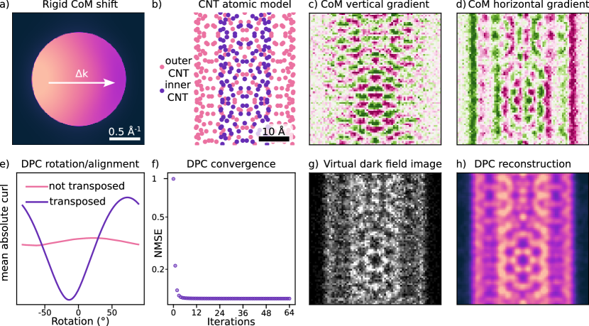
Figure 2: a) Schematic showing center of mass shifts when probe interacts with sample. b) Atomic model of double walled chiral carbon nanotube. Virtual CoM images along c) vertical- and d) horizontal-directions with green and purple indicating + and - shifts respectively. e) Mean CoM curl as a function of real-space/reciprocal-space rotation and alignment. f) Convergence of iterative DPC algorithm. g) Virtual dark field image and h) iterative DPC reconstruction.

2.2 Preprocessing and Results

Due to the helical path accelerated electrons take along the optic axis, as well as the positioning of the detector in the STEM column, there is typically a rotational offset between the real- and reciprocal-space coordinate systems. Since the gradient of the electrostatic potential is by definition a conservative vector field, we can solve for this rotation by minimizing the curl or maximizing the divergence of the vectorial CoM virtual image [15, 23]. These techniques have a $180^{\circ}$ ambiguity in the relative rotation which can be solved by requiring the phase-shift to be positive everywhere except over vacuum (approximately true for most samples), or by performing an independent calibration [15]. While solving for the relative rotation angle is only somewhat important for iterative DPC, ptychographic reconstructions are especially sensitive to this value (see section 4 or Ref. 24).

Figure 2 illustrates our iterative DPC approach with a simulated double-walled carbon nanotube (CNT) structure (fig. 2b). We introduce a -17^∘ rotational offset between real-space and reciprocal-space and transpose the two axes of the diffraction intensities. This transpose is common to many experimental set-ups depending on the detector readout and STEM scanning direction, and can be solved using DPC with the same curl minimization approach. The rotationally-aligned and transposed CoM images are shown in fig. 2c-d. The mean absolute curl algorithm indeed recovers the proper alignment (fig. 2e), as seen by the CoM image contrast being aligned with the $\hat{x}$- and $\hat{y}$-axes respectively. The convergence profile of our DPC reconstruction is shown in fig. 2f, illustrating a large drop off in error after the first few iterations. Comparing the virtual dark field image in fig. 2g and the iterative DPC reconstruction in fig. 2h from the same dataset, we can observe how much more information rich the iterative DPC reconstruction is for this dataset.

There are several advantages to using iterative DPC for recovering sample-induced phase-shifts. First, it is a relatively straightforward and computationally-inexpensive technique, so it can be used to quickly characterize the phase of the sample. Moreover, similar to other phase-contrast techniques, it is fairly dose-efficient and enables linear contrast, although care is needed for any kind of quantitative analysis. Iterative DPC reconstructions only solve for the phase of the sample and do not deconvolve the probe’s wavefunction. Therefore, any aberrations in the probe, including defocus, will be imparted in the reconstruction. The transfer function for iterative DPC reconstructions is peaked around the convergence angle of the incident beam, and information transfer is poor at low and high spatial frequencies  [4]. These artifacts can be ameliorated through the incorporation of high and low pass filters. In fig. 2f, we use a low pass filter of 1.5Å^-1. Masking of the diffraction patterns to include only the bright field disk can also help remove artifacts in DPC reconstructions. Lastly, the real-space resolution of the reconstruction is limited by the real-space step size of the STEM probe, placing stringent sampling requirements during data-acquisition.

3 Parallax Imaging

Despite the benefits described in section 2 of using iterative DPC for phase retrieval in 4D-STEM datasets, the reconstruction quality is limited by the aberrations in the incident electron probe. Figure 3b illustrates an iterative DPC reconstruction for the same CNT structure with a defocused probe. Unlike in fig. 2, it is not possible to resolve atomic features, despite using similar sampling. As we will see in section 4, it is often beneficial to deliberately impart aberrations (specifically defocus) into the probe as a way of relaxing stringent sampling requirements. However, good estimates of these low-order aberrations are necessary for high-quality reconstructions and are often hard to obtain during data acquisition. In this section, we present another phase retrieval technique, termed parallax imaging, which can provide estimates of the aberration coefficients for highly-aberrated probes, and in doing so more faithfully reconstruct the phase imparted by the sample with depth-sectioning resolution [25]. This approach is also referred to as tilt-corrected bright field STEM (tc-BF STEM) and has been demonstrated as an effective phase contrast imaging approach for biological samples [26, 27]. The parallax imaging method can be thought of a weak-phase approximation to the more general scattering matrix reconstruction methods [28, 29, 30].

Each pixel in the diffracted bright field disk can be thought of as a plane wave of electrons which impacted the sample at a slightly different angle, up to a maximum tilt given by the convergence semiangle. For highly-defocused probes, this is geometrically equivalent to different positions on the sample surface, and is related to the “stellar parallax” phenomenon in astronomy [31, 32]. Figure 3a illustrates the phenomenon for the simulated CNT sample shown in fig. 2b. The two virtual images of the CNT created from the different bright field pixels, coloured purple and pink respectively, highlight the relative shift and tilt of the CNT structure. Note that while the virtual images are shown at infinite dose to visually highlight the effect, the algorithm is robust to low dose conditions as we demonstrate below.

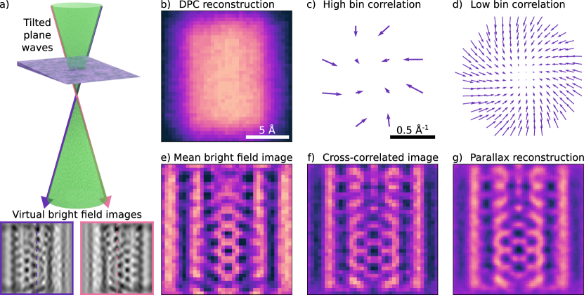
Figure 3: (a) Parallax schematic. Virtual images from individual positions on the central disk represent incoming plane waves at different angles, which appear as a specimen shift. Vertical dashed lines added at field of view midpoint as guides to the eye. (b) Iterative DPC reconstruction does not work well for defocused probes. (c-d) Vector fields for aligning images at different levels of binnning. (e) Mean bright field image and (f) cross-correlated and CTF-corrected image show strong contrast from nanotube. (g) Upsampling to recover the full parallax reconstruction higlights the higher resolution reconstruction.

3.1 Inverse Problem Formalism

We start by forming a virtual image from each pixel within the bright field disk. As discussed above, each of these virtual images will be offset and can be computationally aligned to the center pixel using a geometric parallax operator which we describe here. In short, the operator corrects the geometric intercepts of each virtual image to be properly focused by aligning the virtual images. In our iterative algorithm, we start with a heavily-binned dataset to enable alignment of low-dose datasets and progressively decrease the amount of binning, using the previous iteration’s shifts as a starting point for cross-correlating the virtual images. Figure 3c shows the relative shifts of the virtual images with a high degree of binning, and as we iteratively decrease the level of binning, we recover a finely-sampled vector field used to align the simulated CNT dataset (fig. 3d). The high signal to noise mean bright field image is show in fig. 3e.

Let the final cross-correlation image vector shifts, $\boldsymbol{w}(\boldsymbol{k})$, be denoted by the real-valued array $W\in\mathbb{R}^{G\times 2}$, where $G$ is the number of bright field pixels with initial pixel positions, $\boldsymbol{u}(\boldsymbol{k})$, denoted by $U\in\mathbb{R}^{G\times 2}$. We wish to recover the parallax operator $H\in\mathbb{R}^{2\times 2}$ which relates $U$ and $W$, according to:

$$UH=W.$$ (4)

We use a least-squares estimate of the solution $\hat{H}$:

$$\hat{H} =\left(U^{T}U\right)^{-1}U^{T}W.$$ (5)

The parallax operator can then be separated into rotation $T$ and radial components $S$ using the polar decomposition in eq. 6. These polar and radial components can be manipulated further to recover the rotation $\theta$, negative defocus $C_{1}$, astigmatism $A_{1}^{x}/A_{1}^{y}$:

$$\hat{H} =TS,$$ (6)

where

$$S =\begin{bmatrix}C^{\prime}_{1}&A^{\prime}_{1}\\ A^{\prime\prime}_{1}&C^{\prime\prime}_{1}\end{bmatrix},\quad T=\begin{bmatrix}cos(\theta)&sin(\theta)\\ -sin(\theta)&cos(\theta)\end{bmatrix},$$ (7)

$$C_{1} =\frac{C^{\prime}_{1}+C^{\prime\prime}_{1}}{2},\quad A_{1}^{x}=\frac{A^{\prime}_{1}-A^{\prime\prime}_{1}}{2},\quad\text{and}\;A_{1}^{y}=\frac{A^{\prime}_{1}+A^{\prime\prime}_{1}}{2}.$$ (8)

Note that we can also fit higher order aberrations given a sufficiently accurate measurement of $w$, as each aberration will modulate the image shifts[33]. A similar method to the above steps can be used to measure aberrations in STEM probes in order to facilitate their correction [34].

We can use our low-order aberrations estimates to apply a contrast transfer function (CTF) correction to the reconstruction(fig. 3f). The virtual images can be upsampled before aligning using a kernel-density estimation of the vector field [35], creating a high signal-to-noise reconstruction with the blurring from the defocus removed (fig. 3g).

3.2 Results

The final upsampled reconstruction in fig. 3g illustrates the phase of the simulated CNT dataset. This is a dose-efficient technique since it uses all the scattered information inside the bright field disk. Especially for low dose datasets, it can be helpful to keep the binning high but still use an iterative approach to converge alignments.

More complex deconvolution of signal in the bright field disk is possible through scattering matrix reconstruction, which has been used for 3D-reconstructions of thicker samples [36]. Similarly, with a large convergence angle, the depth-of-field is improved, and the parallax operator can be applied to the upsampled aligned reconstruction to study the out of plane structure of materials [37].

Overall, parallax imaging is a dose-efficient and relatively computationally-inexpensive approach for recovering the phase of specimens in a defocused dataset. Unlike iterative DPC, the resolution of the upsampled reconstruction is not scan step-size limited, but instead is equal to the convergence angle similarly to other phase contrast STEM methods [38]. For low-dose experiments with weakly scattering samples, parallax additionally provides a good estimate for low-order aberrations, especially when there are sufficient pixels within the bright field disk to allow for high binning.

4 Single-slice Ptychography

Electron ptychography was proposed by Walter Hoppe in 1969 [39, 40, 41], with the first STEM proof-of-principle some 25 years later demonstrating the advantages of the method over other phase retrieval techniques in achieving resolution beyond the ‘information limit’ [42]. These early methods developed into two non-iterative algorithms still in-use today, namely single side-band (SSB) [43] and Wigner-distribution deconvolution (WDD) [44]. While these techniques enable dose-efficient imaging at high resolution, they require stringent sampling conditions in both real- and reciprocal-space. In what follows, we instead focus on iterative ptychographic techniques which relax these requirements.

Compared to the phase-retrieval algorithms introduced in sections 2 and 3, the iterative ptychographic algorithms described below offer two distinct advantages. First, since both the sample transmission function and the incoming- wave illumination are jointly reconstructed, the algorithms can overcome the resolution limitations set by residual aberrations. In-fact, low-order aberrations such as defocus are often deliberately introduced during ptychographic data acquisitions to increase probe overlap and thus information redundancy (see section 4.3), enabling dose fractionation and faster acquisition speeds. Secondly, since the reconstruction resolution is set by the largest acquired spatial frequency in the diffraction intensities (see section 4.2), this enables super-resolution imaging and relaxes stringent sampling constraints during data acquisition. Despite these advantages, iterative ptychographic reconstructions require more complex algorithms and are significantly more computationally-expensive, and the reconstruction can fail if the experiment does not contain sufficient redundancy [45].

4.1 Inverse Problem Formalism

In this section, we setup the inverse problem for the simplest ptychographic formulation and adjust the forward and adjoint operators as appropriate in each of the following sections to capture more complex scattering physics. While as we saw in sections 2 and 3, in typical 4D-STEM experiments diffraction intensities are acquired on a 2D raster scan, this is not strictly required and unnecessarily complicates ptychographic notation. Instead, in the following sections we consider a dataset, $I(\boldsymbol{R}_{m},\boldsymbol{k})=I_{m}(\boldsymbol{k})$, of diffraction intensity measurements collected from $M$ probe positions, $\boldsymbol{R}_{m}$. Single-slice ptychography assumes the exit-wave, $\psi_{m}(\boldsymbol{r})$, is given by a simple multiplication of the complex-valued incoming-wave and the complex-valued sample transmission function, henceforth referred to as the “probe,” $\mathcal{P}(\boldsymbol{r})$, and “object,” $\mathcal{O}(\boldsymbol{r}-\boldsymbol{R}_{m})$, respectively, propagated to the farfield detector:

$$\psi_{m}(\boldsymbol{r}) =\Pi_{O}\left[\mathcal{P},\mathcal{O}\right]=\mathcal{P}(\boldsymbol{r})\mathcal{O}(\boldsymbol{r}-\boldsymbol{R}_{m})$$ (9)

$$J_{m}(\boldsymbol{k}) =\left|\mathcal{F}\left[\psi_{m}(\boldsymbol{r})\right]\right|^{2},$$ (10)

where $\Pi_{O}$ is referred to as the "overlap projection" and $J_{m}(\boldsymbol{k})$ is the estimated model intensity at probe position $\boldsymbol{R}_{m}$. The inverse problem is to find probe and object operators which minimize the distance from the measured diffraction intensities given by an appropriate error metric such as:

$$\mathcal{E}=\left(\sum_{m}\sum_{\boldsymbol{k}}I_{m}(\boldsymbol{k})\right)^{-1}\left(\sum_{m}\sum_{\boldsymbol{k}}\left|\sqrt{I_{m}(\boldsymbol{k})}-\sqrt{J_{m}(\boldsymbol{k})}\right|^{2}\right).$$ (11)

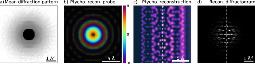
Figure 4: Single-slice ptychographic reconstruction of simulated double-walled carbon nanotube showing a) the mean diffraction pattern using finite dose of $10^{6}$e^-/Ų, b) the reconstructed probe using a $150\textup{\AA}$ initial defocus, c) the reconstructed object and d) spatial frequencies against the simulated ground truth. In c) and d) we compare the ground-truth potential (left) and the reconstruction (right).

From the many existing algorithms to solve this inverse problem [1, 12, 13, 46, 47], we have implemented stochastic gradient descent and proximal gradient solvers due to their robustness and intuitive geometric interpretation respectively. The first step for both is recognizing that the Euclidean projection of the model estimate to the given data, i.e. the minimal modification to the complex-valued exit-wave to satisfy the measured intensities, is given by simply replacing its Fourier amplitude with the square-root of the measured intensity while retaining its phase [1]:

$$\Pi_{F}\left[\psi_{m}(\boldsymbol{r})\right]=\mathcal{F}^{-1}\left[\sqrt{I_{m}(\boldsymbol{k})}\mathcal{F}[\psi_{m}(\boldsymbol{r})]/\sqrt{J_{m}(\boldsymbol{k})}\right],$$ (12)

where $\Pi_{F}$ is referred to as the “Fourier projection.” This allows us to define the appropriate gradient and adjoint operators for the stochastic gradient descent and proximal gradient solvers respectively:

(Stochastic Gradient Descent)

$$\Delta\psi_{m}^{\mathrm{GD}}(\boldsymbol{r}) =\Pi_{F}\left[\psi_{m}(\boldsymbol{r})\right]-\psi_{m}(\boldsymbol{r})$$ (14)

$$\mathcal{O}^{\prime}(\boldsymbol{r}) =\mathcal{O}(\boldsymbol{r})+\beta\biggl{(}||\mathcal{P}(\boldsymbol{r})||_{\alpha}\biggr{)}^{-1}\biggl{(}\sum_{m\in\mathcal{M}}\mathcal{P}^{*}(\boldsymbol{r})\Delta\psi_{m}^{\mathrm{GD}}(\boldsymbol{r})\biggr{)}$$ (15)

$$\mathcal{P}^{\prime}(\boldsymbol{r}) =\mathcal{P}(\boldsymbol{r})+\beta\biggl{(}||\mathcal{O}(\boldsymbol{r}-\boldsymbol{R}_{m})||_{\alpha}\biggr{)}^{-1}\biggl{(}\sum_{m\in\mathcal{M}}\mathcal{O}^{*}(\boldsymbol{r}-\boldsymbol{R}_{m})\Delta\psi_{m}^{\mathrm{GD}}(\boldsymbol{r})\biggr{)},$$ (16)

(Generalized Projections)

$$\Delta\psi_{m}^{\mathrm{PS}}(\boldsymbol{r}) =(1-a-b)\Delta\psi_{m}^{\mathrm{PS}}(\boldsymbol{r})+a\psi_{m}(\boldsymbol{r})+b\Pi_{F}\left[c\psi_{m}(\boldsymbol{r})+(1-c)\Delta\psi_{m}^{\mathrm{PS}}(\boldsymbol{r})\right]$$ (17)

$$\mathcal{O}^{\prime}(\boldsymbol{r}) =\biggl{(}||\mathcal{P}(\boldsymbol{r})||_{\alpha}\biggr{)}^{-1}\biggl{(}\sum_{m}\mathcal{P}^{*}(\boldsymbol{r})\Delta\psi_{m}^{\mathrm{PS}}(\boldsymbol{r})\biggr{)}$$ (18)

$$\mathcal{P}^{\prime}(\boldsymbol{r}) =\biggl{(}||\mathcal{O}(\boldsymbol{r}-\boldsymbol{R}_{m})||_{\alpha}\biggr{)}^{-1}\biggl{(}\sum_{m}\mathcal{O}^{*}(\boldsymbol{r}-\boldsymbol{R}_{m})\Delta\psi_{m}^{\mathrm{PS}}(\boldsymbol{r})\biggr{)},$$ (19)

where $$\beta \mathcal{M} \left(a,b,c\right) ||\cdot||_{\alpha}$$ is the gradient-descent step-size, denotes a batch of probe positions, parameterize a family of projection algorithms, and the normalization is given by:

$$||\cdot||_{\alpha} =(1-\alpha)\sum_{m(\in\mathcal{M})}|\cdot|^{2}+\alpha\sum_{m(\in\mathcal{M})}|\cdot|_{\mathrm{max}}^{2}.$$ (20)

4.2 Numerical Implementation and Preprocessing

In order to efficiently solve the system of eqs. 14, 15, 16, 17, 18 and 19 the object, probe, and exit-wave functions introduced in section 4.1 need to be stored numerically as equisampled arrays. This introduces sampling requirements during data acquisition and reconstruction which control the numerical accuracy, computational cost, and final reconstruction resolution.

The acquired diffraction intensities are stored in the real-valued array, $I\in\mathbb{R}^{M\times Q\times Q}$, for an array of probe positions, $R\in\mathbb{R}^{M\times 2}$. Note that, to avoid resampling the diffraction intensities, we equivalently rotate and transpose the probe positions during preprocessing as necessary to match the reciprocal-space coordinate system (see section 2).

The reciprocal-space pixel size, $\Delta k$, defines the real-space extent, $e=1/\Delta k$, of the complex-valued probe array, $P\in\mathbb{C}^{Q\times Q}$, where $e$ has to be large enough to comfortably fit the (often aberrated) probe without wrap-around artifacts. The largest acquired spatial frequency, $2k_{\mathrm{max}}=\Delta k*Q$, defines the reconstruction real-space pixel size, $\Delta x=1/(2k_{\mathrm{max}})$, which together with the positions of the rotated/transposed probe positions define the object field-of-view in pixels. The probe can be initialized with an estimate of the aberrations and a vacuum probe measurement of the aperture or a guess of the semiangle of the probe. The object array is then padded by as much as half the probe extent to define the size of the complex-valued array, $O\in\mathbb{C}^{S\times T}$, such that $S,T\geq Q$ (see fig. 1).

In evaluating expressions of the form $\psi_{m}(\boldsymbol{r})=\mathcal{P}(\boldsymbol{r})\mathcal{O}(\boldsymbol{r}-\boldsymbol{R}_{m})$, $Q\times Q$ region-of-interest patches are extracted from the larger $S\times T$ object array centered around $\boldsymbol{R}_{m}$ rounded to the nearest pixel and multiplied by the probe array Fourier-shifted by any remaining sub-pixel offsets, and stored in the complex-valued exit-waves array, $\psi\in\mathbb{C}^{M\times Q\times Q}$. Finally, note that the diffraction intensities, probe, and exit-waves are all internally stored as top-left corner-centered arrays to enable the unambiguous centering of even and odd dimension datasets and compatibility with fast Fourier transform libraries.

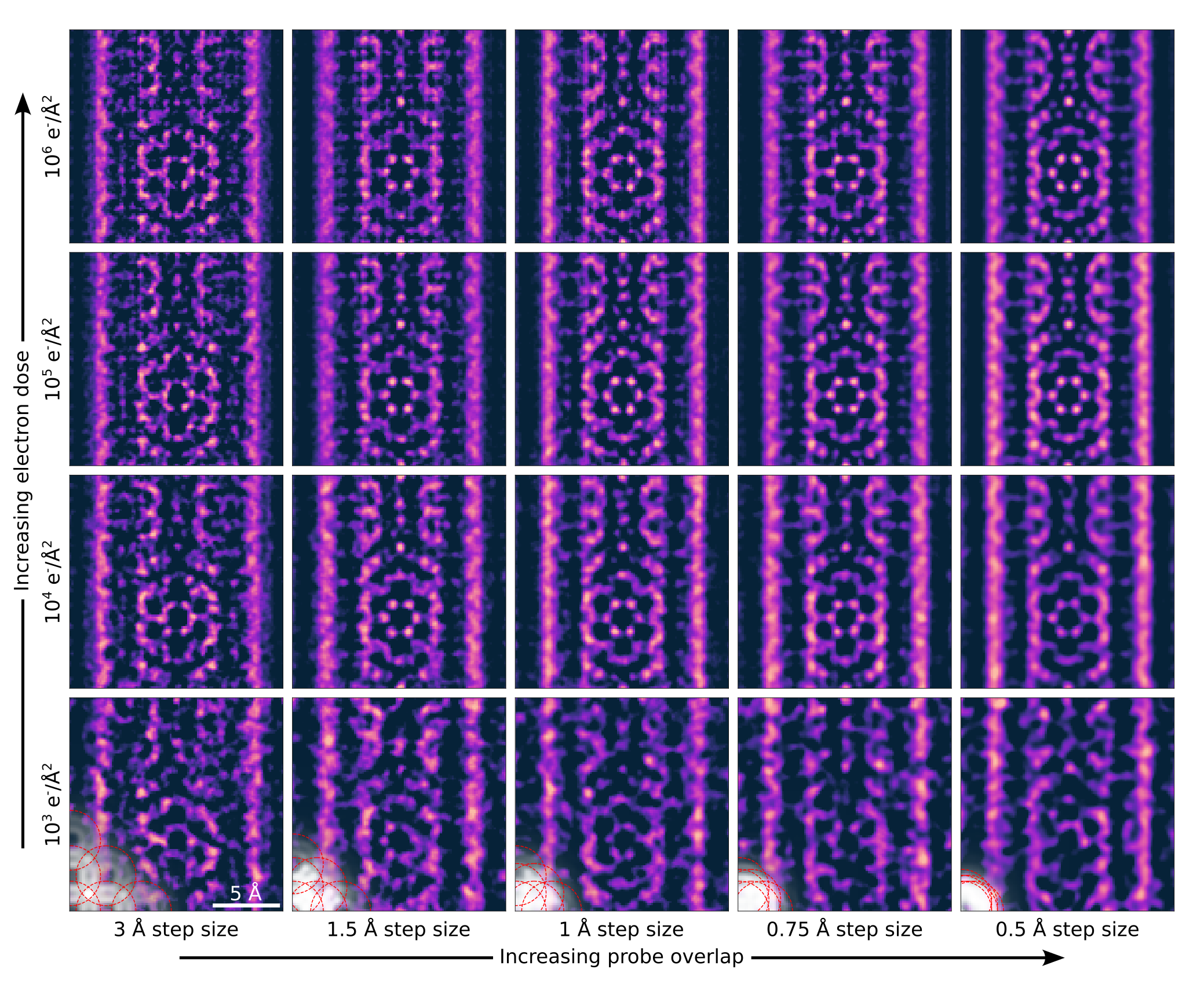
Figure 5: Dependence of single-slice ptychographic reconstruction quality on finite electron dose (rows) and probe overlap (columns). Decreasing probe overlap results in high-frequency artifacts, while decreasing electron dose results in loss of atomic features.

4.3 Probe Overlap and Finite Dose

Consider the same double-walled CNT dataset reconstructed in sections 2 and 3, simulated using $150\textup{\AA}$ defocus and a $1\textup{\AA}$ scan step-size. Figure 4 highlights the improvement ptychography achieves over both iterative DPC and parallax imaging, by enabling super-resolution set by the largest acquired spatial frequency. While $k_{\mathrm{max}}$ determines the resolution limit of the reconstruction, the extent of real-space probe-overlap and the dynamic range of the diffraction intensities control the redundancy in the dataset and ultimately the quality of the reconstructed phase. Due to the high dose and large $k_{\mathrm{max}}$ used in the simulation, ptychography performs better than other imaging approaches.

There are two ways to increase probe-overlap, while maintaining the same spatial resolution: i) decreasing the scan step-size between adjacent probes, or ii) increasing the size of the real-space probe, e.g. by defocusing further or using a smaller probe convergence angle. The former strategy is the most straight-forward, but necessitates larger acquisition times and dataset sizes. The latter strategy can be quite effective however is limited both in using larger defocus, which requires larger region-of-interest arrays to avoid wrap-around artifacts, and smaller convergence angles, which change the effective transfer of information.

Figure 5 illustrates the dependence on reconstruction quality by starting with the same dataset as fig. 4 (shown on the top-right tile) and decreasing the electron dose moving vertically down and decreasing the probe overlap moving horizontally to the left. While the reconstruction quality deteriorates along both these axes, it is interesting to note the difference in the two failure modes. Decreasing the probe overlap at high dose (top row moving left) results in high-frequency artifacts, while decreasing the electron dose at large overlap (rightmost column moving down) results in substantial loss of atomic features. It should also be noted that achieving both high electron-dose and large probe overlap is often experimentally challenging for dose-sensitive samples.

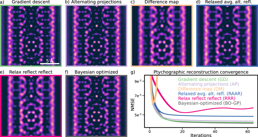
Figure 6: Comparison between various ptychographic reconstruction algorithms. For diverging algorithms such as c) DM and e) RRR, the lowest-error reconstruction is displayed instead. g) Convergence comparison, illustrating how Bayesian optimization can be used to tune the projection set hyperparameters.

4.4 Reconstruction Algorithms Comparison

Electron ptychography is a high-dimensional, non-convex inverse problem over the complex numbers. As such, rigorous proofs of convergence and comparisons between different algorithms are few and far between. In this section, we instead comment on the use of batching in the stochastic gradient descent solver, and various well-known projection-set algorithms based on empirical observations.

First, note that when the batch size in eqs. 14, 15 and 16 is equal to a single probe position, $\mathcal{M}=1$, the stochastic gradient descent algorithm reduces to a regularized version of the well-known extended ptychographic iterative engine (e-PIE) [46, 47], and when $\mathcal{M}=M$ the algorithm is no longer stochastic. For simulated datasets with high electron dose, we find that using a vanishing normalization parameter, $\alpha\to 0$, achieves the lowest error. For low-dose experimental datasets, we almost always observe better behavior as $\alpha\to 1$. While in general we find that using as many probe positions as the available memory permits, $\mathcal{M}\to M$, appears to be both more accurate as well as computationally more performant, we note that using fewer probe positions per iteration allows the algorithm to converge the probe faster. This is particularly important for mixed-state ptychography, which we elaborate further in section 5.

The scalar parameters $\left(a,b,c\right)$ introduced in eqs. 17, 15 and 16 describe a whole family of projection set algorithms, with specific values encoding well-known named algorithms such as alternating projections (AP, $a=0,b=1,c=1$) [48], difference-map (DM, $a=-1,b=1,c=2$) [49], relaxed averaged alternating reflections (RAAR, $a=1-2\gamma,b=\gamma,c=2$) [50], and relax reflect reflect (RRR, $a=-\gamma,b=\gamma,c=2$)[51]. We make the following observations, summarized in fig. 6:

1. The AP (fig. 6b) or “error-reduction” algorithm is very similar to the gradient descent algorithm when $\mathcal{M}=M$ and $\beta=1$ (fig. 6a).

2. While the DM algorithm (fig. 6c), a special case of alternating direction method of multipliers (ADMM) [14], tends to diverge for most datasets we have investigated, variants of the algorithm with relaxation parameters namely RAAR (fig. 6d) and RRR (fig. 6e) show better convergence behaviour.

3. The space of parameters defined by $\left(a,b,c\right)$ lends itself well to dataset-specific hyper-parameter tuning. Figure 6g uses Bayesian optimization with gaussian processes to arrive at a set of parameters with better convergence properties $\left(a=-0.34,b=0.47,c=1.1\right)$. This optimization is further discussed in section 8.4.

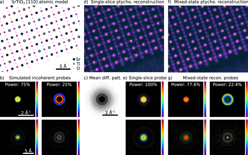
Figure 7: Mixed-state ptychographic reconstruction of simulated STO [110] slab a-c) showing d-e) the breakdown of single-slice ptychography on datasets with partial coherence, and f-g) the much better fidelity reconstruction using mixed-state ptychography with two orthogonal probes.

5 Mixed-state ptychography

The formalism developed in section 4 is capable of reconstructing the probe aperture and aberrations for coherent illumination. However, the transfer of information in 4D-STEM, and thus the quality of ptychographic reconstructions, is often limited by imperfections in the imaging system resulting in partial temporal and spatial coherence [52]. Figure 7 illustrates this breakdown for a synthetic dataset of a STO [110] slab (fig. 7a), simulated by incoherently adding diffraction intensities simulated with a circular aperture between 0-10 mrad (fig. 7b, left) and an annular aperture between 10-20 mrad (fig. 7b, right) with $75\%$ and $25\%$ weights respectively. The single-slice ptychographic reconstruction shown in fig. 7d-e, attempts to dump the partial coherence information in the object while using a single probe aperture, which degrades the reconstruction quality.

While one approach to remedy this could be to adjust our forward operator to include parametric models of partial coherence, it has recently been shown that modeling the probe as a linear combination of pure quantum states can effectively capture partial coherence and provides greater flexibility [53, 45]. In order to capture this, we modify our forward operator in eqs. 9 and 10 to read:

$$\psi_{m}^{(l)}(\boldsymbol{r}) =\Pi_{O}\left[\mathcal{P}^{(l)},\mathcal{O}\right]=\mathcal{P}^{(l)}(\boldsymbol{r})\mathcal{O}(\boldsymbol{r}-\boldsymbol{R}_{m})$$ (21)

$$J_{m}(\boldsymbol{k}) =\sum_{l}\left|\mathcal{F}\left[\psi_{m}^{(l)}(\boldsymbol{r})\right]\right|^{2},$$ (22)

with the Fourier projection and adjoint operators in eqs. 12, 14, 15, 16, 17, 18 and 19 applying mutatis mutandis. Equation 22 holds for $L$ orthogonal probe functions $\left\{\mathcal{P}^{(l)}\right\}$, a constraint which is not a-priori guaranteed by the adjoint operator and must instead be imposed at every iteration. We implement a computationally-efficient variant of the orthogonal probe relaxation (OPR) algorithm [54], which uses the eigenvectors of the pairwise probe functions dot-product instead of computing the singular value decomposition:

$$A_{ij} =\sum_{\boldsymbol{r}}\mathcal{P}^{(i)*}(\boldsymbol{r})\mathcal{P}^{(j)}(\boldsymbol{r})=U\Lambda U^{\dagger}$$ (23)

$$\mathcal{P}^{(i)^{\prime}}(\boldsymbol{r}) =\sum_{j}U_{ij}\mathcal{P}^{(j)}(\boldsymbol{r}).$$ (24)

Figure 7f-g demonstrates the utility of the mixed-state formalism on the same STO [110] dataset reconstructed using a mixture of two orthogonal probe functions. The algorithm successfully manages to separate the circular and annular apertures (fig. 7g), resulting in a much sharper reconstructed object (fig. 7f) as compared to fig. 7d. Finally, as alluded to earlier, the ability of the algorithm to successfully partition and orthogonalize the probe intensities strongly depends on the batch size $\mathcal{M}$. Using a smaller batch size, such that (on-average) probe positions do not overlap substantially, ensures the algorithm performs repeated adjoint and orthogonalization steps leading to more accurate probe intensities, albeit at an increased computational-cost.

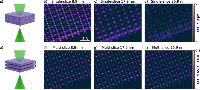
Figure 8: a-d) Single-slice and e-h) multi-slice reconstructions of simulated STO [110] slabs of various thicknesses, highlighting the breakdown of single-slice ptychography for “thick” strongly-scattering samples and the linearity of multi-slice ptychography.

6 Multi-slice ptychography

The forward models introduced so far in sections 4 and 5 assume the exit-waves are given by a simple multiplication of the incoming-wave and the object. While this is a convenient approximation for weakly-scattering or thin samples, it breaks down for multiple-scattering or thick samples as the illumination profile changes significantly as a function of depth due to dynamical scattering and free-space propagation [55]. To account for these effects, multi-slice ptychography approximates the object as a stack of $N$ slices [56], each thin-enough to satisfy the multiplicative assumption (eq. 9), and modifies the forward operator to apply alternating transmission and propagation steps:

$$\psi_{m}^{(n)}(\boldsymbol{r}) =\Pi_{O}\left[\phi_{m}^{(n)},\mathcal{O}^{(n)}\right]=\phi_{m}^{(n)}(\boldsymbol{r})\mathcal{O}^{(n)}(\boldsymbol{r}-\boldsymbol{R}_{m}),$$ (25)

where

$$\phi_{m}^{(1)}(\boldsymbol{r}) =\mathcal{P}(\boldsymbol{r})$$ (26)

$$\phi_{m}^{(n)}(\boldsymbol{r}) =\mathrm{Prop}_{\Delta z_{n-1}}\left[\psi_{m}^{(n-1)}(\boldsymbol{r})\right]\quad\forall n\geq 2.$$ (27)

$\phi_{m}^{(n)}(\boldsymbol{r})$ and $\mathcal{O}_{m}^{(n)}(\boldsymbol{r}-\boldsymbol{R}_{m})$ are the incoming-wave illumination and sample transmission functions evaluated at slice $n$, $\Delta z_{n}$ represents the thickness between slices $n$ and $n+1$, and the free-space propagator is defined according to:

$$\mathrm{Prop}_{\Delta z}\left[\cdot\right] =\mathcal{F}^{-1}\left[G_{\Delta z}(\boldsymbol{q})\mathcal{F}\left[\cdot\right]\right]$$ (28)

$$G_{\Delta z}(\boldsymbol{q}) =\mathrm{exp}\left(-i\pi\lambda\left|q\right|^{2}\Delta z\right),$$ (29)

where $\lambda$ is the electron wavelength. Note that for $N$ slices, we perform $N$ transmission steps but only $N-1$ propagation steps by convention to recover the single-slice formalism for $N=1$.

Starting from the last exit-wave ($n=N$) and working backwards, the adjoint operator is similarly modified to read, e.g. for the stochastic gradient descent algorithm:

$$\mathcal{O}^{(n)^{\prime}}(\boldsymbol{r}) =\mathcal{O}^{(n)}(\boldsymbol{r})+\beta\biggl{(}||\phi_{m}^{(n)}(\boldsymbol{r})||_{\alpha}\biggr{)}^{-1}\biggl{(}\sum_{m\in\mathcal{M}}\phi_{m}^{(n)*}(\boldsymbol{r})\Delta\psi_{m}^{(n)}(\boldsymbol{r})\biggr{)}$$ (30)

$$\mathcal{P}^{\prime}(\boldsymbol{r}) =\mathcal{P}(\boldsymbol{r})+\beta\biggl{(}||\mathcal{O}^{(1)}(\boldsymbol{r}-\boldsymbol{R}_{m})||_{\alpha}\biggr{)}^{-1}\biggl{(}\sum_{m\in\mathcal{M}}\mathcal{O}^{(1)*}(\boldsymbol{r}-\boldsymbol{R}_{m})\Delta\psi_{m}^{(1)}(\boldsymbol{r})\biggr{)},$$ (31)

where

$$\Delta\psi_{m}^{(N)}(\boldsymbol{r}) =\Pi_{F}\left[\psi_{m}^{(N)}(\boldsymbol{r})\right]-\psi_{m}^{(N)}(\boldsymbol{r})$$ (32)

$$\Delta\psi_{m}^{(n)}(\boldsymbol{r}) =\mathrm{Prop}_{-\Delta z_{n}}\left[\Delta\psi_{m}^{(n+1)}(\boldsymbol{r})\mathcal{O}^{(n+1)*}(\boldsymbol{r}-\boldsymbol{R}_{m})\right]\quad\forall n<N.$$ (33)

Note that this is fundamentally different than both the 3D e-PIE [56] and maximum-likelihood [57] formalisms, as we do not take gradient steps at each slice, but rather back-propagate a single gradient step evaluated at the detector plane.

Figure 8 highlights the advantage of multi-slice ptychography for thick samples when the multiplicative assumption breaks down. In fig. 8a-d, we examine the same field of view as fig. 7a at various thicknesses using the single slice algorithm introduced in section 4. Already at 8.9 nm the multiplicative assumption breaks down – which can be seen from the doughnut-like appearance of the strongly scattering Strontium columns, indicative of phase wrapping. The reconstructions for thicker samples are further degraded (fig. 8c-d). By contrast, the multi-slice algorithm introduced above is able to recover the correct sample potential (fig. 8e-h), for thicknesses as large as 26.9 nm. Specifically, here we use 1.1 nm thick slices for each reconstruction with strong regularization along the beam direction, requiring all slices to have equal phase shifts. Finally, we note that the mean slice phase for the various thicknesses in fig. 8f-h are plotted on the same color scale, highlighting the linearity of the reconstruction.

Recently, multi-slice electron ptychography has been used to both achieve sub 20pm atomic-resolution limited by thermal vibrations [58], as well as demonstrate nanometer depth-resolution of dopant and vacancy concentrations [58, 59]. Proper regularization along the beam direction is essential for multislice reconstructions, and will discussed more in section 8.1. In addition, high doses are required to get sufficient signal to noise to recover depth-dependent information.

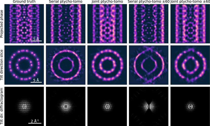
Figure 9: Serial and joint ptychography-tomography reconstructions of simulated double walled CNT, highlighting the importance of missing-wedge artifacts in serial ptychography-tomography, in contrast with the effective regularization of the missing-wedge in joint ptychography-tomography.

7 Joint Ptychography-Tomography

The depth-sectioning capabilities afforded by multi-slice ptychography discussed in section 6, provide limited resolution along the beam direction [58]. An alternative approach, with a rich literature in electron microscopy, is tilting the sample to obtain multiple two-dimensional projections and reconstructing them tomographically to obtain three-dimensional sample information [60].

While traditional STEM electron tomography techniques most often use the inelastically-scattered electrons hitting the high-angle annular dark field (HAADF) detector, which is not sensitive to light atoms, recent work has successfully reconstructed the three-dimensional atomic structure of a heterogeneous sample containing light elements using electron ptychography [61]. In particular, the authors collected a tilt-series of 4D-STEM datasets of a double-walled CNT containing Zr-Te nanostructures and performed mixed-state ptychographic reconstructions for each tilt-angle, which were then reconstructed tomographically to obtain a three-dimensional volume. We will refer to this technique as serial ptychography-tomography, due to the sequential fashion in which the reconstructions are performed. Figure 9 illustrates this technique for a simulated tilt-series along the long-axis of the simulated CNT model shown in fig. 2b with six-degree increments. While the full tilt-series reconstruction (fig. 9, second column) shows sufficient reconstruction quality to trace atoms, the missing wedge artifacts shown in the fourth column of fig. 9 severely degrade the reconstruction quality.

In addition to being much more dose-efficient as compared to HAADF tomography, serial ptychography-tomography can take advantage of the aforementioned benefits of various flavours of ptychography to reconstruct thicker samples with partial coherence. However, it still suffers from common tomographic artifacts such as the missing-wedge.

An alternative, even more dose-efficient, technique is to perform joint ptychography-tomography whereby the three-dimensional volume is reconstructed directly from the 4D-STEM tilt-series dataset [62]. The recently proposed technique, also referred to as multi-slice electron tomography, extends multi-slice ptychography by successively rotating the three-dimensional object estimate, such that the beam direction is aligned with the z-axis for each tilt, and updating the intensity along z- “super” slices using eqs. 30, 31, 32 and 33. The advantages of jointly updating the three-dimensional volume directly are shown in the third and fifth columns of fig. 9 for the full tilt-series and 60^∘ missing-wedge series respectively. In particular the additional angular redundancy in the dataset, combined with effective regularization section 8, enable the reconstruction to efficiently fill in information along the missing-wedge direction (fig. 9, bottom-right panel), resulting in an overall superior reconstruction.

8 4D-STEM Specific Experimental Considerations

The non-convexity and high-dimensionality of the ptychographic inverse problems described in sections 4, 5, 6 and 7 make them particularly hard to converge, especially in the presence of experimental noise. Additionally, the algorithms are not guaranteed to converge to optimal or unique solutions. This can be in-part remedied using effective regularization, which reduce the dimensionality of the available solution-space or constrain ill-posed optimization problems.

While some of these regularizations can be implemented by adding additional priors or penalty terms in the loss function (eq. 11) directly, this can often result in increased computational complexity for the gradient step. Instead, we implement a “projected” gradient approach, whereby we first take unconstrained gradient steps using for example eqs. 14, 15, 15, 17, 18 and 19 and then, at every iteration, project the current probe and object estimates to feasible sets subject to the constraints described below. This can be significantly more efficient computationally, as long as the constraint projections are computationally inexpensive to evaluate at every iteration. In general, as little regularization as possible should be applied to avoid spurious artifacts in the probe and object reconstructions.

8.1 Object regularization

Object regularization includes ensuring the reconstructed object is smooth, using Gaussian or Butterworth filters in real- and reciprocal-space respectively, as well as total variation denoising. These smoothing filters can be applied both in the plane of the object and along the beam-direction for multi-slice and joint ptychography-tomography. For accurate recovery of slices, multi-slice ptychography in particular requires regularization along the beam-direction [58]. The strongest regularization is that all slices are identical. This strict assumption can be relaxed by instead enforcing first-order total variation denoising, allowing for non-identical slices.

Separating the phase and amplitude components of the complex-valued reconstructed object is a challenge in electron ptychography. For weakly-scattering objects (or equivalently sufficiently thin slices of strongly-scattering objects in multi-slice ptychography), the amplitude of the reconstructed object should vary negligibly from unity. As such, we can reduce the solution-space dimensionality in half by employing the strong-phase approximation and constraining the amplitude to unity at each iteration. Taking this a step further, the object itself can be stored as the real-valued potential directly, $\mathcal{O}(\boldsymbol{r})=\mathrm{e}^{\mathrm{i}V(\boldsymbol{r})}$. In addition to the obvious memory efficiencies this affords, it further allows us to impose additional regularization constraints on the potential directly. Notably atomic potentials are, by nature, non-negative and thus we can enforce positivity by clipping negative values to zero. Moreover, positivity can be combined with shrinkage filters, whereby a constant phase-shift is subtracted from the current estimate at each iteration prior to zero-clipping, to promote atomicity by forcing the background to zero.

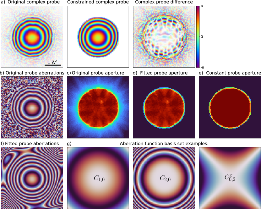
Figure 10: 4D-STEM specific probe regularizations. a) Unphysical reconstructed probe illustrating intensity “leakage” outside the probe aperture, probe-object mixing given by the eight-fold symmetry features, and non-smooth aberration surface. The probe can be separated to b) aberration surface and c) aperture functions. The probe aperture can be constrained to d) remove intensity outside the aperture and e) exhibit flat-field intensity inside the aperture. Similarly, the probe aberration surface, can be fitted to a linear combination of g) low-order aberrations to produce a f) smooth estimate of the surface. Panel a) also shows a comparison between the complex-valued unconstrained probe (left) and constrained probe (middle), together with their difference (right).

8.2 Probe regularization

Similarly, the probe estimate can be constrained using physical regularizations, such as a fixed probe aperture, a smooth phase aberration surface, and center-of-mass fixing. Currently, we support two ways of initializing the probe aperture: either using a vacuum measurement or using an estimate of the probe semiangle, i.e. a perfect circular aperture. In general, a high signal-to-noise vacuum measurement of the probe aperture is important for probe regularization and dataset calibration. This can be acquired by averaging several diffraction intensity measurements over a vacuum region with the same experimental parameters as the 4D-STEM dataset.

One common artifact in ptychographic reconstructions is probe-object mixing (fig. 10a), where object features from the scattered diffraction intensities appear in the Fourier amplitude of the probe. This can be ameliorated by using a vacuum measurement of the probe aperture, effectively reducing the solution-space dimensionality by half. If such a measurement is not available (and cannot be estimated from a vacuum region of the field of view), then the current Fourier probe estimate can be fitted to an angularly-varying sigmoid function to suppress intensity outside the probe aperture and ensure a top-hat intensity inside the aperture (fig. 10c-e).

Moreover, the probe aberration surface is expected to be smoothly-varying. This is not guaranteed a-priori (fig. 10b), and can instead be imposed as an iterative constraint. An elegant way of enforcing this is to fit the aberration surface $\chi(\boldsymbol{k})$ to a linear combination basis-set of low-order aberrations [63]:

$$\chi(\boldsymbol{k})=\sum_{m=0}\sum_{n=0}\left(\lambda\;k\right)^{2m+n}\left[C_{m,n}^{x}\cos{\left[n\times\mathrm{atan2}\left(k_{y},k_{x}\right)\right]}+C_{m,n}^{y}\sin{\left[n\times\mathrm{atan2}\left(k_{y},k_{x}\right)\right]}\right],$$ (34)

where $C_{m,n}^{x},C_{m,n}^{y}$ are the coefficients of the two orthogonal aberrations of order (m, n) in units of radians, and $\mathrm{atan2}\left(k_{y},k_{x}\right)$ is the arctangent function which returns the correct sign in all quadrants. Note that when $n=0$ the aberration is radially symmetric (e.g. constant value, defocus, spherical aberration) and no $C_{m,0}^{y}$ term is necessary. Figure 10f-g show the fitted aberration surface and some basis set examples respectively. Finally, we note that for this to work, the aberration surface needs to be phase-unwrapped first.

8.3 Probe positions updates

Lastly, the probe positions estimate can be refined during the ptychographic reconstruction as well as constrained to fit a linear drift distortion model. Drift in STEM data acquisition causes the real probe positions to deviate from the ideal raster positions [64]. In general, faster 4D-STEM data acquisition times, which are determined by detector read out speeds, step size, and the required field of view, lead to fewer artifacts in the positions of the probes.

During ptychographic reconstruction we can refine our probe positions estimate, using a gradient step on the intensity measurements in parallel [65]. This results in a displacement vector for each probe position, which can be further constrained by fitting the displacement vectors to a six-parameter (x-scaling, y-scaling, shear, rotation, x-translation, y-translation) global affine transformation. Because the ptychography algorithms rely on overlap between adjacent probe positions, fine tuning or probe positions is required for object convergence.

8.4 Hyper-parameter Tuning

In order to successfully perform a ptychographic reconstruction of experimental data, it is necessary that certain experimental parameters be known to high precision, particularly the raster scan step size and the reciprocal pixel size of the diffraction patterns. Other parameters, such as the defocus and real-space/reciprocal-space rotation angle, are either refined during reconstruction or relatively simple to determine from the dataset, but still affect the convergence. In addition, reconstruction parameters such as the step size, batch size, and regularization strengths, also impact the quality of the reconstruction. In order to find the optimum values of both experimental and reconstruction parameters that give the highest quality reconstruction of a dataset, we have implemented an optimizer using the Bayesian optimization (BO) with Gaussian processes (GP) algorithm. BO-GP is commonly used in the tuning of hyperparameters for machine learning [66], and has been successfully applied to ptychography both for parameter tuning [67] and directly as a procedure for iterative phase retrieval [68]. The BO-GP algorithm models the function to be minimized as a mixture of Gaussian processes, and chooses evaluation points through a mixture of exploration of unsampled regions of the parameter space and exploitation of local minima of the GP model. Our implementation provides a simple interface for specifying optimization parameters, and the optimization is performed by the BO-GP routine provided by scikit-optimize [69]. Various reconstruction quality metrics can be used as the objective function of the optimizer, including the final data error of the reconstruction as well as the contrast, entropy, or total variation, of the reconstructed object.

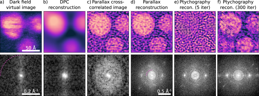
Figure 11: a) Dark field imaging, b) DPC reconstructions, and c) parallax reconstructions are all limited by real-space sampling. d) Subpixel alignment of parallax and upsampling allows for reconstruction of atomic features. e) Ptychography after 5 iterations shows high spatial frequencies. f) After 300 iterations, the reconstruction converges the low spatial frequencies and provides the highest resolution reconstruction.

9 Experimental Results

The previous sections use simulated datasets to illustrate the differences between various phase retrieval algorithms and highlight the effects of common experimental parameters such as scan sampling and finite dose on the reconstruction quality. As emphasized in the introduction, our phase retrieval algorithm implementations and specifically the regularization constraints introduced in section 8 were designed to be robust against common experimental artifacts. To this end, in this section we test our implementations on a sample of gold nanoparticles on a carbon grid.

This dataset is not optimized for conventional high-resolution imaging for two reasons. First, the real-space step size is 2 Å, which is not fine enough to capture atomic features in this nanoparticle. Second the dataset was acquired with a large defocus to optimize conditions for parallax and ptychography reconstructions. LABEL:{fig:gold}a shows the dark field from the field of view, and it is not possible to see the fine features in the nanoparticles. Similarly, it is not possible to see structural features of the gold nanoparticles using an iterative DPC reconstruction (LABEL:{fig:gold}b). However, both dark field imaging and the iterative DPC reconstruction recover the low-spatial frequencies well by clearly showing the difference in phase between the gold nanoparticles and the carbon support film. The iterative DPC reconstruction provides the additional advantage that it can solve for the real/reciprocal coordinate system rotation as 13^∘ with no need to transpose the data.

The parallax reconstruction in LABEL:{fig:gold}c is an improvement over the iterative DPC and dark field modalities as it shows some of the fine features in the nanoparticles. Moreover, the parallax reconstruction estimate for the real/reciprocal coordinate system rotation is 12^∘, which is nearly identical to the iterative DPC estimate. It also estimates the defocus as 106 nm. The upsampled parallax reconstructions in LABEL:{fig:gold}d show a dramatic improvement in resolution as compared to the other bright field techniques (LABEL:{fig:gold}a-c). Making use of the subpixel alignment information in the parallax reconstruction and upsampling the real-space images, it is possible to recover atomic resolution structural information.

The rotation and defocus estimates can be used to initialize the single slice ptychographic reconstruction, which is shown in fig. 11e-f. In these methods, although high frequency features in the gold nanoparticles are quick to appear, the lower frequencies are slower to converge. This is evident in comparing fig. 11e and f. After only 5 iterations, we can observe the lattice features in the gold nanoparticles, but the relative phase shifts between the gold and carbon have not yet converged.

Convergence of these ptychographic reconstructions required regularization. A vacuum probe measurement was taken for this dataset, so the probe Fourier aperture could be constrained. To account for sample drift and scan distortion artifacts, position correction was applied during the first 150 iterations. Ultimately, the ptychographic reconstruction is improved over the upsampled parallax, albeit at increased computational cost and optimization of parameters.

10 Methods

STEM simulations were preformed using the abTEM package [70]. The double-walled CNT structure was constructed using the atomic simulation environment (ASE) package [71]. The iterative DPC simulations shown in fig. 2 were performed at 80kV with a 25 mrad probe with zero defocus using 12 frozen-phonon configurations with a displacement standard deviation of .075 Å. The scan step size and reciprocal sampling were 0.25 Å and 2.5 mrad respectively. A rotation of 17^∘ and transpose, as well as finite dose of $10^{5}$e^-/Ų were added to the data. The parallax simulations shown in fig. 3 used the same parameters but a 0.5Å step size, 0.7 mrad reciprocal-space sampling, 20 nm of defocus, and no transpose was added. The single-slice ptychography simulations shown in figs. 4 and 6 used the same parameters but a 0.5Å step size, 2.5 mrad reciprocal-space sampling, 15 nm of defocus, and finite dose $10^{6}$e^-/Ų. The scan step sizes and finite electron doses in fig. 5 varied between 0.5 Å  to 3.0Å and $10^{3}$e^-/Ų to $10^{7}$e^-/Ų respectively. Finally, the tilt series shown in fig. 9 was comprised of (30) 20 tilt angles from ($\pm$90^∘) $\pm$60^∘ in 6^∘ increments for the case (without) with a missing wedge, and finite dose of $10^{4}$e^-/Ų.

The SrTiO₃ structure was constructed using ASE from a unit-cell file taken from the materials project [72]. The mixed-state and multi-slice ptychography simulations shown in figs. 7 and 8 were perfomed at 200kV with a 20 mrad probe, 10 nm of defocus, 12 frozen-phonon configurations with a displacement standard deviation of 0.1 Å, and sampling of 0.5 Å and 1.8 mrad in real and reciprocal-space respectively. The incoherent mixed-state dataset was obtained by adding the intensities of two independent simulations using the simulated probes shown in fig. 7b with a 3:1 ratio and a finite electron dose of $10^{5}$e^-/ Ų. The thickness of the SrTiO₃ sample used in multi-slice simulations was set by repeating unit cells of the structure along the beam direction matching the thicknesses described in the text, and using a finite electron dose of $10^{4}$e^-/ Ų.

The experimental dataset was taken on a Titan double-corrected microscope at 300kV in energy-filtered TEM mode to minimize the effect of inelastic scattering with approximately $10^{5}$e^-/ Ų. A 17 mrad convergence angle probe introduced with 100 nm of defocus was used and a real-space step size of 2 Å. The 4D-STEM dataset was acquired with the K3 camera in counting mode using the full detector and 4x binning.

11 Summary

In this paper we have outlined a number of 4D-STEM based techniques for phase retrieval, as well as introduced a number of 4D-STEM specific regularizations. The optimal reconstruction technique will depend on the sample, experimental parameters, and scientific question. Iterative DPC works best for in-focus datasets, with strict sampling requirements set by the scan-step size. Nonetheless, this is the least computationally expensive and most straightforward technique, and iterative DPC may provide sufficient information for many samples. Parallax reconstructions require only slightly increased computation than iterative DPC, but enable resolution higher than the real-space sampling, as well as accurrate estimates of low-order aberrations. Finally, ptychographic techniques provide the highest resolution reconstructions, at increased computational cost and reconstruction parameter complexity.

12 Acknowledgements

We thank Lena Kourkoutis for her inspirational ideas and support of this project. GV acknowledges support from the Miller Institute for Basic Research in Science, and in-particular fruitful discussions with Joel E. Moore of the University of California, Berkeley. SMR acknowledges support from the IIN Ryan Fellowship and the 3M Northwestern Graduate Research Fellowship, and the U.S. Department of Energy, Office of Science, Office of Workforce Development for Teachers and Scientists, Office of Science Graduate Student Research (SCGSR) program. The SCGSR program is administered by the Oak Ridge Institute for Science and Education for the DOE under contract number DE-SC0014664. BHS acknowledges support from the Toyota Research Foundation. CO and SMR acknowledge support from the US Department of Energy Early Career Research Program. This work made use of the electron microscopy facility of the Platform for the Accelerated Realization, Analysis, and Discovery of Interface Materials (PARADIM), which is supported by the National Science Foundation under Cooperative Agreement No. DMR-2039380. This work received support from the SHyNE Resource (NSF ECCS-2025633). Work at the Molecular Foundry was supported by the Office of Science, Office of Basic Energy Sciences, of the U.S. Department of Energy under contract number DE-AC02-05CH11231.

13 Competing Interests

The authors declare that they have no competing interests.

	Symbol		Definition
General
	$\mathcal{F}\left[\cdot\right]$	$=$	Two-dimensional Fourier transform operator
	$\real\left\{\cdot\right\}$	$=$	Real part of complex-valued expression
	$\boldsymbol{r}$	$=$	Real-space coordinate
	$\boldsymbol{k}$	$=$	Reciprocal-space coordinate
	$\boldsymbol{R}_{m}$	$=$	mth real-space probe position
	$I(\boldsymbol{R}_{m},\boldsymbol{k})=I_{m}(\boldsymbol{k})$	$=$	4D-STEM diffraction intensities
	$\beta$	$=$	Step size
	$\mathcal{E}$	$=$	Error metric
Iterative DPC
	$V(\boldsymbol{r})$	$=$	Electrostatic sample potential
	$\mathcal{I}_{\alpha}^{V}(\boldsymbol{R})$	$=$	Virtual CoM image along cartesian direction $\alpha$
Parallax
	$w(\boldsymbol{k})$	$=$	virtual image shifts
	$u(\boldsymbol{k})$	$=$	position on bright field disk
	$\hat{H}$	$=$	Least squares estimate of $w$ and $u$ relationship
	$S$	$=$	Rotational component of $\hat{H}$
	$T$	$=$	Radial component of $\hat{H}$
	$C_{1}$	$=$	$-\Delta f$, negative defocus
	$A_{1}^{x}$ & $A_{1}^{y}$	$=$	Astigmatism
(Single-slice) Ptychography
	$\mathcal{P}(\boldsymbol{r})=\mathcal{F}^{-1}\left[A(\boldsymbol{k})\mathrm{e}^{-\mathrm{i}\chi(\boldsymbol{k})}\right]$	$=$	Real-space complex-valued probe operator
	$A(\boldsymbol{k})$	$=$	Fourier-space probe aperture
	$\chi(\boldsymbol{k})$	$=$	Fourier-space probe aberration function
	$\mathcal{O}(\boldsymbol{r}-\boldsymbol{R}_{m})=\mathrm{e}^{\mathrm{i}V(\boldsymbol{r}-\boldsymbol{R}_{m})}$	$=$	Real-space complex-valued object operator
	$\Pi_{O}\left[\cdot\right]$	$=$	Overlap projection operator
	$\Pi_{F}\left[\cdot\right]$	$=$	Fourier projection operator
	$\psi_{m}(\boldsymbol{r})$	$=$	Real-space complex-valued exit-waves
	$\Delta\psi_{m}^{\mathrm{GD/PS}}(\boldsymbol{r})$	$=$	Real-space complex-valued exit-waves gradient
	$||\cdot||_{\alpha}$	$=$	$\alpha$-Regularized norm (eq. 20)

Table 1: Nomenclature used in the manuscript. For mixed-state, multi-slice, and joint ptychography-tomography, we try and use consistent notation with the appropriate superscript changes to denote the probe, slice, and tilt indices respectively.

References

- [1] J. R. Fienup, “Phase retrieval algorithms: a comparison,” \JournalTitleApplied optics 21, 2758–2769 (1982).
- [2] F. Zernike, “Phase contrast, a new method for the microscopic observation of transparent objects part ii,” \JournalTitlePhysica 9, 974–986 (1942).
- [3] R. Danev and K. Nagayama, “Transmission electron microscopy with zernike phase plate,” \JournalTitleUltramicroscopy 88, 243–252 (2001).
- [4] N. Dekkers and H. De Lang, “Differential phase contrast in a stem,” \JournalTitleOptik 41, 452–456 (1974).
- [5] J. Rodenburg and A. Maiden, Ptychography (Springer International Publishing, Cham, 2019), pp. 819–904.
- [6] V. Boominathan, J. T. Robinson, L. Waller, and A. Veeraraghavan, “Recent advances in lensless imaging,” \JournalTitleOptica 9, 1–16 (2022).
- [7] T. J. Pennycook, G. T. Martinez, P. D. Nellist, and J. C. Meyer, “High dose efficiency atomic resolution imaging via electron ptychography,” \JournalTitleUltramicroscopy 196, 131–135 (2019).
- [8] L. Zhou, J. Song, J. S. Kim, X. Pei, C. Huang, M. Boyce, L. Mendonça, D. Clare, A. Siebert, C. S. Allen, E. Liberti, D. Stuart, X. Pan, P. D. Nellist, P. Zhang, A. I. Kirkland, and P. Wang, “Low-dose phase retrieval of biological specimens using cryo-electron ptychography,” \JournalTitleNature Communications 11, 2773 (2020).
- [9] A. Scheid, Y. Wang, M. Jung, T. Heil, D. Moia, J. Maier, and P. A. van Aken, “Electron Ptychographic Phase Imaging of Beam-sensitive All-inorganic Halide Perovskites Using Four-dimensional Scanning Transmission Electron Microscopy,” \JournalTitleMicroscopy and Microanalysis 29, 869–878 (2023).
- [10] J. Miao, P. Charalambous, J. Kirz, and D. Sayre, “Extending the methodology of x-ray crystallography to allow imaging of micrometre-sized non-crystalline specimens,” \JournalTitleNature 400, 342–344 (1999).
- [11] C. Ophus, “Four-dimensional scanning transmission electron microscopy (4d-stem): From scanning nanodiffraction to ptychography and beyond,” \JournalTitleMicroscopy and Microanalysis 25, 563–582 (2019).
- [12] J. M. Rodenburg and H. M. L. Faulkner, “A phase retrieval algorithm for shifting illumination,” \JournalTitleApplied Physics Letters 85, 4795–4797 (2004).
- [13] P. Thibault, M. Dierolf, A. Menzel, O. Bunk, C. David, and F. Pfeiffer, “High-resolution scanning x-ray diffraction microscopy,” \JournalTitleScience 321, 379–382 (2008).
- [14] N. Parikh and S. Boyd, “Proximal algorithms,” \JournalTitleFound. Trends Optim. 1, 127–239 (2014).
- [15] B. H. Savitzky, S. E. Zeltmann, L. A. Hughes, H. G. Brown, S. Zhao, P. M. Pelz, T. C. Pekin, E. S. Barnard, J. Donohue, L. R. DaCosta et al., “py4dstem: A software package for four-dimensional scanning transmission electron microscopy data analysis,” \JournalTitleMicroscopy and Microanalysis 27, 712–743 (2021).
- [16] M. C. Cao, Y. Han, Z. Chen, Y. Jiang, K. X. Nguyen, E. Turgut, G. D. Fuchs, and D. A. Muller, “Theory and practice of electron diffraction from single atoms and extended objects using an empad,” \JournalTitleMicroscopy 67, i150–i161 (2018).
- [17] N. Shibata, Y. Kohno, S. D. Findlay, H. Sawada, Y. Kondo, and Y. Ikuhara, “New area detector for atomic-resolution scanning transmission electron microscopy,” \JournalTitleJournal of electron microscopy 59, 473–479 (2010).
- [18] T. Seki, Y. Ikuhara, and N. Shibata, “Toward quantitative electromagnetic field imaging by differential-phase-contrast scanning transmission electron microscopy,” \JournalTitleMicroscopy 70, 148–160 (2021).
- [19] E. Waddell and C. JN, “Linear imaging of strong phase objects using asymmetrical detectors in stem,” \JournalTitleOptik 54, 83–96 (1979).
- [20] K. Müller-Caspary, F. F. Krause, F. Winkler, A. Béché, J. Verbeeck, S. Van Aert, and A. Rosenauer, “Comparison of first moment stem with conventional differential phase contrast and the dependence on electron dose,” \JournalTitleUltramicroscopy 203, 95–104 (2019).
- [21] Z. Li, J. Biskupek, U. Kaiser, and H. Rose, “Integrated differential phase contrast (idpc)-stem utilizing a multi-sector detector for imaging thick samples,” \JournalTitleMicroscopy and Microanalysis 28, 611–621 (2022).
- [22] H. Yang, T. J. Pennycook, and P. D. Nellist, “Efficient phase contrast imaging in stem using a pixelated detector. part ii: Optimisation of imaging conditions,” \JournalTitleUltramicroscopy 151, 232–239 (2015).
- [23] M. J. Zachman, Z. Yang, Y. Du, and M. Chi, “Robust atomic-resolution imaging of lithium in battery materials by center-of-mass scanning transmission electron microscopy,” \JournalTitleACS nano 16, 1358–1367 (2022).
- [24] A. Maiden, M. Humphry, M. Sarahan, B. Kraus, and J. Rodenburg, “An annealing algorithm to correct positioning errors in ptychography,” \JournalTitleUltramicroscopy 120, 64–72 (2012).
- [25] C. Ophus, T. R. Harvey, F. S. Yasin, H. G. Brown, P. M. Pelz, B. H. Savitzky, J. Ciston, and B. J. McMorran, “Advanced phase reconstruction methods enabled by four-dimensional scanning transmission electron microscopy,” \JournalTitleMicroscopy and Microanalysis 25, 10–11 (2019).
- [26] K. A. Spoth, K. X. Nguyen, D. A. Muller, and L. F. Kourkoutis, “Dose-efficient cryo-stem imaging of whole cells using the electron microscope pixel array detector,” \JournalTitleMicroscopy and Microanalysis 23, 804–805 (2017).
- [27] Y. Yu, M. Colletta, K. A. Spoth, D. A. Muller, and L. F. Kourkoutis, “Dose-efficient tcbf-stem with information retrieval beyond the scan sampling rate for imaging frozen-hydrated biological specimens,” \JournalTitleMicroscopy and Microanalysis 28, 1192–1194 (2022).
- [28] H. G. Brown, Z. Chen, M. Weyland, C. Ophus, J. Ciston, L. J. Allen, and S. D. Findlay, “Structure retrieval at atomic resolution in the presence of multiple scattering of the electron probe,” \JournalTitlePhysical review letters 121, 266102 (2018).
- [29] P. M. Pelz, H. G. Brown, S. Stonemeyer, S. D. Findlay, A. Zettl, P. Ercius, Y. Zhang, J. Ciston, M. Scott, and C. Ophus, “Phase-contrast imaging of multiply-scattering extended objects at atomic resolution by reconstruction of the scattering matrix,” \JournalTitlePhysical Review Research 3, 023159 (2021).
- [30] S. D. Findlay, H. G. Brown, P. M. Pelz, C. Ophus, J. Ciston, and L. J. Allen, “Scattering matrix determination in crystalline materials from 4d scanning transmission electron microscopy at a single defocus value,” \JournalTitleMicroscopy and microanalysis 27, 744–757 (2021).
- [31] F. W. Bessel, “Bestimmung der entfernung des 61sten sterns des schwans.” \JournalTitleAstronomische Nachrichten, volume 16, Issue 5, p. 65 16, 65 (1838).
- [32] H. Siebert, “The early search for stellar parallax: Galileo, castelli, and ramponi,” \JournalTitleJournal for the History of Astronomy 36, 251–271 (2005).
- [33] J. Cowley, “Coherent interference in convergent-beam electron diffraction and shadow imaging,” \JournalTitleUltramicroscopy 4, 435–449 (1979).
- [34] A. R. Lupini, P. Wang, P. D. Nellist, A. I. Kirkland, and S. J. Pennycook, “Aberration measurement using the ronchigram contrast transfer function,” \JournalTitleUltramicroscopy 110, 891–898 (2010).
- [35] C. Ophus, J. Ciston, and C. T. Nelson, “Correcting nonlinear drift distortion of scanning probe and scanning transmission electron microscopies from image pairs with orthogonal scan directions,” \JournalTitleUltramicroscopy 162, 1–9 (2016).
- [36] H. G. Brown, P. M. Pelz, S.-L. Hsu, Z. Zhang, R. Ramesh, K. Inzani, E. Sheridan, S. M. Griffin, M. Schloz, T. C. Pekin et al., “A three-dimensional reconstruction algorithm for scanning transmission electron microscopy data from a single sample orientation,” \JournalTitleMicroscopy and Microanalysis 28, 1632–1640 (2022).
- [37] E. Terzoudis-Lumsden, T. Petersen, H. Brown, P. Pelz, C. Ophus, and S. Findlay, “Resolution of virtual depth sectioning from four-dimensional scanning transmission electron microscopy,” \JournalTitleMicroscopy and Microanalysis 29, 1409–1421 (2023).
- [38] C. Ophus, J. Ciston, J. Pierce, T. R. Harvey, J. Chess, B. J. McMorran, C. Czarnik, H. H. Rose, and P. Ercius, “Efficient linear phase contrast in scanning transmission electron microscopy with matched illumination and detector interferometry,” \JournalTitleNature communications 7, 10719 (2016).
- [39] W. Hoppe, “Beugung im inhomogenen Primärstrahlwellenfeld. I. Prinzip einer Phasenmessung von Elektronenbeungungsinterferenzen,” \JournalTitleActa Crystallographica Section A 25, 495–501 (1969).
- [40] W. Hoppe and G. Strube, “Beugung in inhomogenen Primärstrahlenwellenfeld. II. Lichtoptische Analogieversuche zur Phasenmessung von Gitterinterferenzen,” \JournalTitleActa Crystallographica Section A 25, 502–507 (1969).
- [41] W. Hoppe, “Beugung im inhomogenen Primärstrahlwellenfeld. III. Amplituden- und Phasenbestimmung bei unperiodischen Objekten,” \JournalTitleActa Crystallographica Section A 25, 508–514 (1969).
- [42] P. D. Nellist, B. C. McCallum, and J. M. Rodenburg, “Resolution beyond the ’information limit’ in transmission electron microscopy,” \JournalTitleNature 374, 630–632 (1995).
- [43] T. J. Pennycook, A. R. Lupini, H. Yang, M. F. Murfitt, L. Jones, and P. D. Nellist, “Efficient phase contrast imaging in stem using a pixelated detector. part 1: Experimental demonstration at atomic resolution,” \JournalTitleUltramicroscopy 151, 160–167 (2015).
- [44] J. Rodenburg and R. Bates, “The theory of super-resolution electron microscopy via wigner-distribution deconvolution,” \JournalTitlePhilosophical Transactions of the Royal Society of London. Series A: Physical and Engineering Sciences 339, 521–553 (1992).
- [45] Z. Chen, M. Odstrcil, Y. Jiang, Y. Han, M.-H. Chiu, L.-J. Li, and D. A. Muller, “Mixed-state electron ptychography enables sub-angstrom resolution imaging with picometer precision at low dose,” \JournalTitleNature communications 11, 2994 (2020).
- [46] A. M. Maiden and J. M. Rodenburg, “An improved ptychographical phase retrieval algorithm for diffractive imaging,” \JournalTitleUltramicroscopy 109, 1256–1262 (2009).
- [47] A. Maiden, D. Johnson, and P. Li, “Further improvements to the ptychographical iterative engine,” \JournalTitleOptica 4, 736–745 (2017).
- [48] J. von Neumann, “Functional operators, vol. ii, ser,” \JournalTitleAnnals of Mathematics Studies. Princeton Univ. Press (1950).
- [49] V. Elser, “Phase retrieval by iterated projections,” \JournalTitleJOSA A 20, 40–55 (2003).
- [50] D. R. Luke, “Relaxed averaged alternating reflections for diffraction imaging,” \JournalTitleInverse problems 21, 37 (2004).
- [51] V. Elser, “The complexity of bit retrieval,” \JournalTitleIEEE Transactions on Information Theory 64, 412–428 (2017).
- [52] C. Dwyer, R. Erni, and J. Etheridge, “Measurement of effective source distribution and its importance for quantitative interpretation of stem images,” \JournalTitleUltramicroscopy 110, 952–957 (2010).
- [53] P. Thibault and A. Menzel, “Reconstructing state mixtures from diffraction measurements,” \JournalTitleNature 494, 68–71 (2013).
- [54] M. Odstrcil, P. Baksh, S. A. Boden, R. Card, J. E. Chad, J. G. Frey, and W. S. Brocklesby, “Ptychographic coherent diffractive imaging with orthogonal probe relaxation,” \JournalTitleOpt. Express 24, 8360–8369 (2016).
- [55] S. Gao, P. Wang, F. Zhang, G. T. Martinez, P. D. Nellist, X. Pan, and A. I. Kirkland, “Electron ptychographic microscopy for three-dimensional imaging,” \JournalTitleNature communications 8, 163 (2017).
- [56] A. M. Maiden, M. J. Humphry, and J. M. Rodenburg, “Ptychographic transmission microscopy in three dimensions using a multi-slice approach,” \JournalTitleJOSA A 29, 1606–1614 (2012).
- [57] E. H. Tsai, I. Usov, A. Diaz, A. Menzel, and M. Guizar-Sicairos, “X-ray ptychography with extended depth of field,” \JournalTitleOptics express 24, 29089–29108 (2016).
- [58] Z. Chen, Y. Jiang, Y.-T. Shao, M. E. Holtz, M. Odstrčil, M. Guizar-Sicairos, I. Hanke, S. Ganschow, D. G. Schlom, and D. A. Muller, “Electron ptychography achieves atomic-resolution limits set by lattice vibrations,” \JournalTitleScience 372, 826–831 (2021).
- [59] D. Yoon, Y.-T. Shao, Y. Yang, D. Ren, H. D. Abruña, and D. A. Muller, “Imaging Li Vacancies in a Li-Ion Battery Cathode Material by Depth Sectioning Multi-slice Electron Ptychographic Reconstructions,” \JournalTitleMicroscopy and Microanalysis 29, 1263–1264 (2023).
- [60] Y. Yang, C.-C. Chen, M. Scott, C. Ophus, R. Xu, A. Pryor, L. Wu, F. Sun, W. Theis, J. Zhou et al., “Deciphering chemical order/disorder and material properties at the single-atom level,” \JournalTitleNature 542, 75–79 (2017).
- [61] P. M. Pelz, S. Griffin, S. Stonemeyer, D. Popple, H. Devyldere, P. Ercius, A. Zettl, M. C. Scott, and C. Ophus, “Solving complex nanostructures with ptychographic atomic electron tomography,” \JournalTitlearXiv preprint arXiv:2206.08958 (2022).
- [62] J. Lee, M. Lee, Y. Park, C. Ophus, and Y. Yang, “Multislice electron tomography using four-dimensional scanning transmission electron microscopy,” \JournalTitlePhys. Rev. Appl. 19, 054062 (2023).
- [63] C. Ophus, H. I. Rasool, M. Linck, A. Zettl, and J. Ciston, “Automatic software correction of residual aberrations in reconstructed hrtem exit waves of crystalline samples,” \JournalTitleAdvanced Structural and Chemical Imaging 2, 15 (2016).
- [64] C. Ophus, J. Ciston, and C. T. Nelson, “Correcting nonlinear drift distortion of scanning probe and scanning transmission electron microscopies from image pairs with orthogonal scan directions,” \JournalTitleUltramicroscopy 162, 1–9 (2016).
- [65] P. Dwivedi, A. Konijnenberg, S. Pereira, and H. Urbach, “Lateral position correction in ptychography using the gradient of intensity patterns,” \JournalTitleUltramicroscopy 192, 29–36 (2018).
- [66] J. Bergstra, R. Bardenet, Y. Bengio, and B. Kégl, “Algorithms for hyper-parameter optimization,” \JournalTitleAdvances in neural information processing systems 24 (2011).
- [67] M. C. Cao, Z. Chen, Y. Jiang, and Y. Han, “Automatic parameter selection for electron ptychography via Bayesian optimization,” \JournalTitleScientific Reports 12, 12284 (2022).
- [68] P. M. Pelz, W. X. Qiu, R. Bücker, G. Kassier, and R. J. D. Miller, “Low-dose cryo electron ptychography via non-convex Bayesian optimization,” \JournalTitleScientific Reports 7, 9883 (2017).
- [69] T. Head, M. Kumar, H. Nahrstaedt, G. Louppe, and I. Shcherbatyi, “scikit-optimize/scikit-optimize,” (2021).
- [70] J. Madsen and T. Susi, “The abtem code: transmission electron microscopy from first principles,” \JournalTitleOpen Research Europe 1, 24 (2021).
- [71] A. H. Larsen, J. J. Mortensen, J. Blomqvist, I. E. Castelli, R. Christensen, M. Dułak, J. Friis, M. N. Groves, B. Hammer, C. Hargus et al., “The atomic simulation environment—a python library for working with atoms,” \JournalTitleJournal of Physics: Condensed Matter 29, 273002 (2017).
- [72] A. Jain, S. P. Ong, G. Hautier, W. Chen, W. D. Richards, S. Dacek, S. Cholia, D. Gunter, D. Skinner, G. Ceder et al., “Commentary: The materials project: A materials genome approach to accelerating materials innovation,” \JournalTitleAPL materials 1 (2013).