Facilitating Practical Fault-tolerant Quantum Computing Based on Color Codes

Abstract

Color code is a promising topological code for fault-tolerant quantum computing. Insufficient research on color code has delayed its practical application. In this work, we address several key issues to facilitate practical fault-tolerant quantum computing based on color codes. First, by introducing decoding graphs with error-rate-related weights, we improve the threshold of the triangular color code under the standard circuit-level noise model to $0.47\%$, narrowing the gap to that of the surface code. Second, we investigate the circuit-level decoding strategy of color code lattice surgery, which is crucial for performing logical operations in a quantum computer with two-dimensional architecture. Lastly, the state injection protocol of triangular color code is proposed, offering an optimal logical error rate compared to any other state injection protocol of the CSS code, which is beneficial for increasing the efficiency of magic state distillation.

I Introduction

Quantum computation provides a potential way to solve classically intractable problems, such as integer factorization [1] and simulation of large quantum systems [2, 3]. To enable the practical large-scale quantum computation, quantum error correction (QEC) is the crucial technique that protects information against the noise by encoding physical qubits into logical qubits of a certain type of QEC code [4, 5, 6].

Much of the current work focuses on the stabilizer code [7], a well-studied QEC code. As a type of stabilizer code, topological codes [8, 9] including color codes [10, 11] and surface codes [12] draw extra attention since they are compatible with the real hardware limited by the local constraints in the two-dimensional (2-D) architecture. Compared to surface code, the advantage of color code is that it encodes a logical qubit with fewer physical qubits and can implement logical Clifford gates transversally. However, it has long been believed that the circuit-level threshold of color codes is about an order of magnitude lower than that of surface codes, which is a significant reason why color codes fall behind in the competition with surface codes [13, 14, 15, 16].

When performing logical operations on 2-D hardware, lattice surgery [17, 13, 18, 19, 20] is currently the mainstream scheme since it retains locality constraints and offers lower overhead compared to braiding scheme [21]. Lattice surgery implements logical gates, including Clifford gates and non-Clifford gates, through fault-tolerant measurements of multi-body logical Pauli operators. Recent work shows that lattice surgery of color codes can further reduce the time cost by measuring an arbitrary pair of commuting logical Pauli operators in parallel [18], which offers additional evidence of the advantage of color codes. Moreover, in the lattice surgery of surface codes, measurements involving Pauli $Y$ operators typically needs to introduce twist defects, which increase the requirement of device connectivity and resource costs [22, 23]. In spite of Ref [24] that proposes twist-free lattice surgery scheme, it still requires additional space and time overhead. While in color code lattice surgery, the difficulties of measuring arbitrary logical Pauli operators are almost the same, since they can transform into each other through transversal single-qubit Clifford gates.

Another focus of fault-tolerant quantum computing is the magic state, which is used to perform logical non-Clifford gates such as $T$ gates [25]. Obtaining high-fidelity magic states requires an expensive process called magic state distillation [26, 27, 28]. The first step of magic state distillation is injecting a physical magic state into a logical state. The quality of the initial magic states from state injection will remarkably affect the error rate of the output state after distillation. Several previous literatures have demonstrated that magic states from a surface code state injection protocol have a better fidelity than the operations used to construct them [29, 30, 31]. Surprisingly, there is almost no research on a well-designed state injection protocol of color codes despite the enormous potential impact.

There are three main results in this paper. First, the threshold of the triangular color code under circuit-level noise model in the previous work [32] $0.37\%$ is improved. Based on the project decoder [33, 32], we construct new decoding graphs by an automatic procedure and introduce error-rate-related weights to implement more accurate matching by minimum weight perfect matching (MWPM) algorithm [34, 35]. The numerical results show that the threshold is around $0.47\%$, which is the highest threshold of 2-D color code under circuit-level noise to the best of our knowledge. Second, we propose a decoding algorithm of color code lattice surgery. This algorithm is applicable to common lattice surgery schemes on triangular color code including the recent parallel scheme in Ref [18], and is expected to be generalized to other types of color codes. We simulate an example in which logical operators $X_{L}\otimes X_{L}$ and $Z_{L}\otimes Z_{L}$ are measured in parallel and find that the space-like effective code distance is slightly less than that the time-like one. Lastly, we investigate state injection of color code and give a protocol based on post-selection. The performance of our protocol is superior to the existing state injection protocols of surface codes in terms of logical error rates, post-selection success rates, and process complexity. Furthermore, it has been proven that the logical error rate of this protocol is optimal compared to any state injection protocol in CSS code [36, 37]. We also discuss how to design a proper post-selection scheme by the correlation coefficients of syndrome changes and the occurrence of logical errors.

The remaining paper is organized as follows. Sec II reviews some basic but important concepts in fault-tolerant quantum computation and specifies notations used in this paper. Sec III introduces the improved color code decoding strategy and presents the numerical evidence of the threshold increase. In Sec IV, we describe the circuit-level decoding of color code lattice surgery and discuss its universal applicability. Then in Sec V, the state injection protocol of color codes is proposed, where we use a theorem to summarize its optimality. Finally, the conclusion and outlook are presented in Sec VI.

II Preliminaries

In this section we briefly review some important background materials for 2-D color codes, which are referred throughout the paper. Sec II.1 introduces the basic definitions and notations about triangular color codes. In Sec II.2, we discuss the Pauli-based computation and how the lattice surgery performs in the 2-D color codes. In Sec II.3, we review another key problem of the fault-tolerant quantum computation – magic state distillation. Lastly, the details of the circuit-level noise model are presented in Sec II.4, which is the premise of the following discussions and numerical results.

II.1 Triangular color codes and notations

2-D color codes are topological QEC codes constructed in a three-colorable and trivalent lattice. In this paper, we focus on the triangular color code which is defined in the hexagonal lattice $\mathcal{L}_{0}$ with three boundaries. Let us denote the sets of vertices, edges and faces of a lattice (or a graph) $\mathcal{L}$ by $V(\mathcal{L})$, $E(\mathcal{L})$ and $F(\mathcal{L})$, respectively. As inllustrated in Fig. 1a, each data qubit of the triangular color code is placed in a vertex $v\in V(\mathcal{L}_{0})$, and each face $f\in F(\mathcal{L}_{0})$ corresponds to two stabilizer generators $S^{X}_{f}=\otimes_{v\in f}X_{v}$ and $S^{Z}_{f}=\otimes_{v\in f}Z_{v}$, respectively. The logical code space is the simultaneous eigenspace of all the stabilizers and the measurement results of all stabilizer generators is a binary string called syndrome. The triangular color code encodes one logical qubit, whose logical Pauli operators can be defined as the tensor product of Pauli operators supported by a string in the boundary. The Pauli weight of the logical Pauli operator is the code distance, denoted by $d$. Note that color codes are Calderbank-Shor-Steane stabilizer codes and self-dual, i.e., the supports of $S^{X}_{f}$ and $S^{Z}_{f}$ are the same. Hence, the $X$ or $Z$ errors can be corrected separately in an analogous manner.

Given the primal lattice $\mathcal{L}_{0}$ of the color code, it is convenient to discuss the decoding problem on its dual lattice $\mathcal{L^{*}}$. In the dual lattice $\mathcal{L^{*}}$, data qubits are placed on faces and stabilizer generators correspond to the vertices except for three boundary vertices $v_{R}$, $v_{G}$ and $v_{B}$. The dual lattice of the triangular color code with distance $d=7$ is illustrated in Fig. 1b. We use $\epsilon\subseteq F(\mathcal{L^{*}})$ to denote the set of faces identified with qubits affected by $X$ (or $Z$) errors and $\sigma\subseteq V(\mathcal{L^{*}})$ to denote the vertex set in which the identified stabilizer generators anticommutes with the error supported by $\epsilon$.

We also need to define three restricted lattices $\mathcal{L}^{*}_{C}$, where $C\in\{RG,RB,GB\}$. The restricted lattice, say $\mathcal{L}^{*}_{RG}$, is obtained from $\mathcal{L^{*}}$ by removing all blue vertices of $\mathcal{L^{*}}$ as well as all the edge and faces incident to the removed vertices.

Moreover, for color code decoding under the circuit level noise model, 3-D lattices or graphs are usually used where the vertical direction is the time layers and in each time layer is a 2-D lattice. We use $v_{i}^{t}$ to denote the vertex in a 3-D lattice or graph, where $t\in\mathbb{Z}^{+}$ is the number of layers in which $v_{i}^{t}$ is located and $v_{i}$ is the projection of $v_{i}^{t}$ on the 2-D lattice. One type of 3-D lattice that we frequently use is $\mathcal{L}\times n$, which is defined by $V(\mathcal{L}\times n)=\{v_{i}^{t}|v_{i}\in V(\mathcal{L}),t=1,2,...,n\}$ and $E(\mathcal{L}\times n)=\{(v_{i}^{t},v_{j}^{t})|(v_{i},v_{j})\in E(\mathcal{L}),t=1,2,...,n\}\cup\{(v_{i}^{t},v_{i}^{t+1})|v_{i}\in V(\mathcal{L}),t=1,2,...,n-1\}$, where $\mathcal{L}$ is a 2-D lattice and $n$ is a positive integer. In particular, we say two edges $e_{1}=(v_{1}^{t_{1}},v_{2}^{t_{2}})$, $e_{2}=(v_{3}^{t_{3}},v_{4}^{t_{4}})$ are parallel in a 3-D lattice if $v_{1}=v_{3}$, $v_{2}=v_{4}$ and $t_{3}-t_{1}=t_{4}-t_{2}$, notated by $e_{1}//e_{2}$.

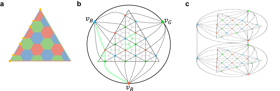
Figure 1: (a) Primal lattice $\mathcal{L}_{0}$ of the triangular color code. Each hexagonal or half-hexagonal face corresponds to two stabilizers which are the tensor products of $X$ and $Z$ supported by the qubits located in the vertices of the face. The logical operator is defined as tensor products of $X$ (or $Z$) supported by the qubits located in a string (colored by yellow). (b) Dual lattice $\mathcal{L}^{*}$ of the triangular color code with $d=7$. The green lines and circles are two examples of paths and corresponding corrections in the decoding. (c) 3-D lattice $\mathcal{L}^{*}\times t$ (here $t=2$). Each layer of $\mathcal{L}^{*}\times t$ is the 2-D dual lattice $\mathcal{L}^{*}$. The corresponding vertices of adjacent layers are connected vertically. To avoid clutter, we only show the vertical connections of three boundary vertices.

Lastly, it is also required to define the path $s$ in a lattice or graph $\mathcal{G}$ to be a sequence of vertices $s=v_{1}^{t_{1}}-v_{2}^{t_{2}}-...-v_{n}^{t_{n}}$, where $(v_{k}^{t_{k}},v_{k+1}^{t_{k+1}})\in E(G)$ for any $k\in{1,2,...,n-1}$. The reverse of $s$ is defined as $\bar{s}=v_{n}^{t_{n}}-v_{n-1}^{t_{n-1}}-...-v_{1}^{t_{1}}$. We refer to $s[k]$ as the $k$th vertex in path $s$ and refer to the first and last vertices as the endpoints of $s$. If an edge $e$ satisfies $e=(s[k],s[k+1])$, we say edge $e$ is on the path $s$. If the two endpoints of path $s$ are the same, we say $s$ is enclosed. In addition, two functions acting on the paths are defined as follows. First, if $s_{1}=v_{1}^{t_{1}}-v_{2}^{t_{2}}-...-v_{n}^{t_{n}}$ and $s_{2}=v_{n+1}^{t_{n+1}}-v_{n+2}^{t_{n+2}}-...-v_{n+m}^{t_{n+m}}$ have the same endpoint, we say $s_{1}$, $s_{2}$ can be connected and $s=s_{1}+s_{2}$ is the connection of $s_{1}$ and $s_{2}$, where $s$ is the sequence of $n+m-1$ vertices satisfying $s[1]-s[2]-...-s[n]=s_{1}$ or $\bar{s}_{1}$, and $s[n]-s[n+1]-...-s[n+m-1]=s_{2}$ or $\bar{s}_{2}$. Second, suppose $s=v_{1}^{t_{1}}-v_{2}^{t_{2}}-...-v_{n}^{t_{n}}$ is a path in a 3-D lattice $\mathcal{L}\times n$, the projection of $s$ is defined as $v_{1}-v_{2}-...-v_{n}$, denoted by ${\rm proj}(s)$, which is a path in the 2-D lattice $\mathcal{L}$. Here the projection is module 2, which means that if an even number of edges on $s$ are projected into the same edge, it is equivalent to deleting this edge in the projection.

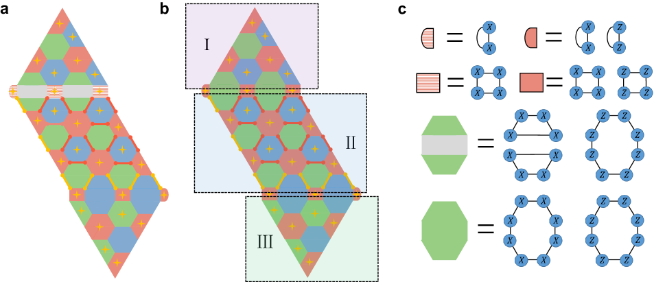
Figure 2: (a) Lattice surgery of triangular color codes for measuring $X_{L}\otimes X_{L}$. The qubits in the middle part are initialized to Bell States (red and yellow pairs). Then the result is the product of the measurement outcomes of starred X-type stabilizers. (b) Lattice surgery of triangular color codes for measuring $X_{L}\otimes X_{L}$ and $Z_{L}\otimes Z_{L}$ in parallel. The results are the product of the measurement outcomes of starred X-type (or Z-type) stabilizers. (c) Specific forms of the stabilizers in the connection parts.

II.2 Color code lattice surgery and Pauli-based computation

Lattice surgery is a measurement-based scheme allowing for efficient implementation of universal gate sets by fault-tolerant logical muti-body Pauli operator measurements. It is especially suitable for 2-D topological quantum codes, such as color code or surface code, since it only requires 2-D qubit layout and local interactions.

For triangular color codes, Fig. 2a shows an example of lattice surgery for measuring $X_{L}\otimes X_{L}$ of two logical qubits. Two triangular logical qubits are merged by ancillary lattice in the middle, where data qubits are initialized to Bell states in pairs. Then the QEC cycles are performed to measure the stabilizers given in Fig. 2c. The outcome of the $X_{L}\otimes X_{L}$ measurement is determined by the product of some stabilizer measurement outcomes, based on $X_{L}\otimes X_{L}=S^{*}B^{*}$, where $S^{*}$ is the product of X-type stabilizers labeled by a star and $B^{*}$ is the stabilizers $X\otimes X$ of yellow Bell states in Fig. 2a. After repeating $d$ rounds of QEC circuits for fault-tolerance, two logical qubits are spilt by measuring their own stabilizers. Based on $X_{L}\otimes X_{L}$ measurement and transversal logical Clifford gates of color codes, one can realize arbitrary 2-qubit logical Pauli operator measurements by lattice surgery.

Different from surface codes, lattice surgery of color codes allows arbitrary pairs of commuting logical Pauli measurements in parallel while the space cost remains the same [18]. For example, keeping the qubit layout in Fig. 2a, parallel measurements of $X_{L}\otimes X_{L}$ and $Z_{L}\otimes Z_{L}$ can be achieved as long as the stabilizers that connect logical qubits and ancillary lattice are replaced with the stabilizers shown in Fig. 2b. Ref [18] and Ref [38] give more general examples of color code lattice surgery with different types of 4-weight and 8-weight stabilizers in the connection parts.

By lattice surgery, one can perform the gate-based computation where a universal gate set is realized by Pauli operator measurements and ancilla qubits [21]. However, with the capacity of measuring arbitrary Pauli operators, a natural way to achieve universal quantum computing is Pauli based computation (PBC) [39].

In the PBC model, a gate-based quantum circuit is equivalent to a series of Pauli operator measurements on initial states $\ket{0^{\otimes n}}$ and ancilla magic states $\ket{m^{\otimes k}}$. To illustrate this, let us start with a Clifford+$T$ circuit in Fig. 3, which is well-known to form a universal gate set. By commuting all $T$ gates to the foreside of the circuit, the Clifford+$T$ circuit is replaced with a series of $\frac{\pi}{8}$ Pauli rotations $P(\frac{\pi}{8})$, followed by Clifford gates $C^{\prime}$ and $Z$-basis measurements. Then a $\pi/8$ Pauli rotation can be realized by Pauli operator measurement and Clifford gates with an ancilla magic state (see Fig. 4a). Lastly, we commute all Clifford gate and $Z$-basis measurements, which transforms $Z$-basis measurements to multi-body Pauli operator measurements. Therefore, we have proven PBC model is equivalent to a universal gate-base computation model.

Note that the outcome of measurement $M_{i}$ may affect subsequent measurements, since there is a Clifford gate $P_{\pi/4}$ controlled by measurement outcome when we perform $P(\frac{\pi}{8})$ gate. Hence, the execution time of the PBC circuit is linearly related to the layers of $P(\frac{\pi}{8})$ gates where $P(\frac{\pi}{8})$ gates commute in the same layer. Some literatures focus on reducing the time overhead. For instance, the time-optimal scheme [40, 20] allows parallelism of the measurement layers by using a large number of ancilla qubits, and the temporally encoded lattice surgery scheme [24] effectively reduces the time of per measurement.

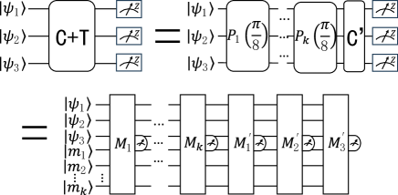
Figure 3: Equivalence of the gate-based quantum computation model and the PBC model. The Clifford circuit is universal for quantum computing. First we commute all the Clifford gates to the right of the circuit and then perform all $P(\frac{\pi}{8})$ gates by introducing $k$ magic states and $k$ multi-body Pauli operator measurements. Lastly, the Clifford gates can be absorbed by the final measurements.

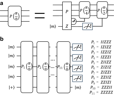
Figure 4: (a) $\pi/8$ rotation gate implemented by consuming a magic state. (b) Circuit of the 15 to 1 magic state distillation protocol. Four magic states are consumed in the initial states and 14 magic states are consumed to implement $P(\frac{\pi}{8})$ gate.

II.3 Magic state distillation

In general, a practical quantum computer requires a universal gate set. According to the Eastin-Knill theorem [41], no QEC code admits a universal and transversal logical gate set. The logical Clifford gates in the topological quantum codes are typically easier to implement by lattice surgery or braiding operations [15, 42]. However, performing non-Clifford logical gates such as a $\pi/8$ Pauli rotation gate $P(\frac{\pi}{8})=e^{-i\pi P/8}$ requires extra resource state $\ket{m}=\ket{0}+e^{i\pi/4}\ket{1}$ called magic state.

Utilizing magic state as ancilla qubit, one can realize a logical gate $P(\frac{\pi}{8})$ by the circuits in Fig. 4a using multi-body Pauli operator measurements and classical controlled Clifford gates. Suppose the Pauli operator measurements and Clifford gates are implemented fault-tolerantly by lattice surgery, the fidelity of the logical gate $P(\frac{\pi}{8})$ is mainly determined by the fidelity of $\ket{m}$. High-fidelity magic states can be produced by several copies of noisier magic states, which is called magic state distillation. Magic state distillation is often considered the most costly part of fault-tolerant quantum computing, even though many efficient protocols are constantly proposed [43, 44, 45, 28, 46].

Here we briefly review the most well-known magic state distillation protocol, the 15 to 1 protocol as an example [20]. This protocol is based on the 15-qubit Reed-Muller code, the smallest QEC code with the transversal $T$ gate [47]. The distillation circuit starts with four magic states $\ket{m}$ and a $\ket{+}$ state, followed by $\pi/8$ Pauli rotation gates and $X$-basis measurements, as shown in Fig. 4b. Since one magic state is consumed in each $\pi/8$ Pauli rotation gate implementation, a total of 15 magic states are consumed to distill one high-fidelity magic state. The errors of at most two of 15 magic states can be detected by the $X$-basis measurements. If any $X$-basis measurement outcome is $-1$, all qubits are discarded and the distillation protocol is restarted. Suppose that every input magic state suffers Z-type Pauli error $Z_{\pi/2}$ with probability $p_{i}$, the error rate of the output magic state is $p_{out}\approx 35p_{i}^{3}$ since there are 35 combinations of three faulty magic states that cannot be detected. If the input magic states suffer $X$, $Y$, $Z$ Pauli errors with probabilities $p_{x}$, $p_{y}$, $p_{z}$ respectively, the output error rate is $p_{out}\approx 35[p_{z}+\frac{(p_{x}+p_{y})}{2}]^{3}$ [28].

Typically, the initial input magic states are produced by a non-fault-tolerant procedure called state injection. This procedure injects an arbitrary physical state $\ket{\psi}=\alpha\ket{0}+\beta\ket{1}$ into the logical state $\ket{\psi_{L}}=\alpha\ket{0_{L}}+\beta\ket{1_{L}}$. The state injection is crucial since the fidelity of the distilled magic states depends strongly on the quality of the initial magic states. For example, in the 15 to 1 distillation protocol, if the error rate of the initial states $p_{i}$ is reduced to $p_{i}/n$, the error rate of the output state is reduced by around $n^{(3^{k})}$ times for $k$ rounds of distillation.

II.4 Qubit layout and circuit-level noise model

Here we introduce the basic assumptions about the qubit layout. The data qubit is placed in each vertex of the primal lattice of triangular color code, and two syndrome qubits are in each colored face for the stabilizer measurements. One of the syndrome qubits is initialized to $\ket{0}$ for measuring the Z-type stabilizer and the other is initialized to $\ket{+}$ for measuring the X-type stabilizer. The syndrome qubits are coupled with data qubits by CNOT gates. Those assumptions run through the following discussions of the color code decoding, lattice surgery and magic state injection.

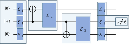
Figure 5: An example of the noisy circuit to prepare a Bell state. We label the noise channels of the initialization errors, two-qubit gate errors, idle errors and measurement errors separately.

It is known that error correcting performance of QEC codes depends largely on noise models. Throughout this paper, the noise model we considered is the circuit-level depolarizing noise model. The depolarizing error channels are defined as:

$$\mathcal{E}_{1}(\rho_{1}) =(1-p)\rho_{1}+(p/3)\sum_{P\in{X,Y,Z}}P\rho_{1}P$$ (1)

$$\mathcal{E}_{2}(\rho_{2}) =(1-p)\rho_{2}+(p/15)$$

$$\times\sum_{\begin{subarray}{c}P_{1},P_{2}\in{I,X,Y,Z},\\ P_{1}\otimes P_{2}\neq I\otimes I\end{subarray}}P_{1}\otimes P_{2}\rho_{2}P_{1}\otimes P_{2},$$

where $\rho_{1}$ and $\rho_{2}$ are single-qubit and two-qubit density matrices respectively and $p$ is the physical error rate.

When simulating a noisy quantum circuit, we approximate every noisy operation by an ideal operation followed by the depolarizing error channel $\mathcal{E}_{1}$ or $\mathcal{E}_{2}$. Specifically, the depolarizing error channels are added to the circuits by the following rules:

(1) add $\mathcal{E}_{1}$ after preparing each $\ket{0}$ or $\ket{1}$ state;

(2) add $\mathcal{E}_{1}$ after each idle operation;

(3) add $\mathcal{E}_{1}$ before each measurement in $Z$- or $X$-basis;

(4) add $\mathcal{E}_{2}$ after each CNOT gate.

A noisy quantum circuit for preparing a bell state is shown in Fig. 5. Note that if a qubit in some step is not acted by any of the preparation, two-qubit gate or measurement while operations of other qubits are being performed, it is assumed to be applied to an idle operation and suffer the error channel $\mathcal{E}_{1}$. In fact, errors from idle operations account for a large portion when we simulate high-weight stabilizer measurement circuit of the color code.

III Improved Color code decoding

This section describes our improved color code decoding strategy and presents numerical results. Our improved decoding strategy is based on the projection decoder [32, 33]. The variation is that, we execute the MWPM algorithm on a graph with error-rate-related weights, rather than the original dual lattice $\mathcal{L^{*}}$. In Sec III.1, we discuss how to construct the decoding graphs and the criterion that a proper CNOT schedule (i.e., the order of the CNOT gates in the QEC circuits) needs to meet. In Sec III.2, we explain the entire process of the decoding algorithm and give the numerical results.

III.1 Decoding graphs and CNOT schedules

When decoding topological QEC codes by the MWPM algorithm, the performance of the decoder is affected by the matching weights. For example, in the surface code, the MWPM algorithm is typically applied in a graph with weights where the weight of the edge is related to the probability of the given pair of syndrome changes. Ref [48] has calculated the probabilities of the six types of edges by categorically analyzing the error in the surface code QEC circuit.

By introducing the error-rate-related weights, the decoding performance increases substantially. Therefore, this inspires us to consider introducing the error-rate-related weights in the color code decoding graph. However, constructing such decoding graphs of color codes faces two main challenges:

(a) The QEC circuit of color codes is deeper and the the qubit array is more complex compared to that of surface codes, which makes analyzing the edge error rate categorically more difficult.

(b) For the surface code, by setting the proper CNOT schedule, a single error in the circuit always causes the two syndrome changes or less. Here a single error means the Pauli error from one depolarizing error channel in the noisy circuit. However, for the color code, because of the high-weight stabilizer measurements and error propagations, a single error may cause syndrome changes of more than two, in which case an error no longer corresponds to just one edge in the decoding graph.

Figure 6: CNOT schedules of stabilizers with different weights used in color code QEC circuits and lattice surgery. The outside and inside numbers are position labels and time orders respectively. The stabilizers on the face along the boundary of a lattice are half of the stabilizers in the figure, following the same time orders.

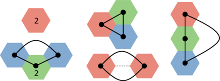
Figure 7: Five possible syndrome changes (colored faces) and their connections (solid lines) of a single error in the color code QEC circuit with the proper CNOT schedule. We only show the projection of the faces, which means that the syndrome changes may come from different time layers. A face labeled 2 indicates that the syndrome changes twice in two consecutive time layers and corresponds a vertical connection.

To address the challenge (a), we designed an automatic procedure to count the syndromes of various errors in the QEC circuit. First, we construct three 3-D decoding graphs $\mathcal{G}_{C}$ ($C\in\{RG,RB,GB\}$), where the vertical dimension is the time layers and in each time layer is a 2-D graph. We assume that the total number of the time layers in the decoding graph $\mathcal{G}_{C}$ is $d+1$ , which corresponds to $d$ rounds of noisy QEC circuits and one perfect QEC circuits round. The vertices of the decoding graph are the same as those in the 3-D restricted lattice $\mathcal{L}^{*}_{C}\times(d+1)$, but the edges are different.

Second, in order to determine the edges in the decoding graph $\mathcal{G}_{C}$, we simulate an ideal QEC circuit attached to a single error in the different positions in the circuit. If the error is located in channel $\mathcal{E}_{1}$, the error is $X$, $Y$ or $Z$. If the error is located in channel $\mathcal{E}_{2}$, the error is one of $P_{1}\otimes P_{2}$ where $P_{1},P_{2}\in{I,X,Y,Z}$ and $P_{1}\otimes P_{2}\neq I\otimes I$. For each possible position and type of error, the procedure simulates the QEC circuit and records the syndrome changes in each simulation.

Suppose that in the decoding graph $\mathcal{G}_{C}$, these recorded vertices are connected in pairs by some rules (see Appendix A for details), and the error $\epsilon$ in one simulation leads to the edge $e$, the weight of $e$ is assigned $w_{e}=-\log\sum_{\epsilon}p_{\epsilon}(e)$, where $p_{\epsilon}(e)=p/3$ if $\epsilon$ is a single-qubit error, otherwise $p_{\epsilon}(e)=p/15$.

Now let us consider challenge (b): how to reduce the number of syndrome changes caused by a single error. In fact, the problem can be dealt with by a proper CNOT schedule. Intuitively, we hope that the multiple errors resulting from a single error propagation are neighbors, so that some syndrome changes can cancel each other out. For example, if an $X$ error in syndrome qubit propagates to two neighbor data qubits, the number of syndrome changes is still 2. In contrast, if two error data qubits are not neighbor, the number of syndrome changes is more than 2. Based on this intuition, we propose a criterion that a proper CNOT schedule needs to meet.

Suppose the position label of the data qubit that is applied $i$th ($i=1,2,3...$) CNOT gate in the time order is $l_{i}$, where $\{l_{i}\}=\{1,2,…,N\}$ are integers fixed on the $N$-weight stabilizer that increases clockwise (see Fig. 6). A proper CNOT schedule holds: given any $i\in\{1,2,…,N\}$, $\forall a,b\in\{l_{i+1},l_{i+2},…,l_{N}\}$, we have $|a-b|\,{\rm mod}\,N\leq N-i$, where $x\,{\rm mod}\,N$ is the modulo function ranged in $[0,N)$. In other words, the criterion guarantees that the syndrome qubit’s error after the $i$th CNOT gate always propagates to the data qubits whose positions $\{l_{i+1},l_{i+2},…,l_{N}\}$ are $N-i$ neighbor positions.

Previous work proposes the optimal CNOT schedule for the triangular color code, which exactly meets the criterion. Therefore, we continue to use this CNOT schedule of 6-weight stabilizers in Fig. 6. It should be noted that the criterion we proposed also applies to higher-weight stabilizer measurements, such as the 8-weight stabilizers used in the lattice surgery (see Sec IV and Fig. 6).

Once the CNOT schedule is given, we can explain how to connect the syndrome changes in pairs of a single error. There are 5 types of syndrome changes of a single error using the optimal CNOT schedule. As explained in Appendix A and Fig 7, the edge $e\in E(\mathcal{G}_{C})$ in three decoding graphs is determined by the connection of the syndrome changes in pair. Except for one type in the bottom left corner, only two syndrome changes occur in each decoding graph at most. Moreover, if the error propagates to the boundary data qubits, one of the vertices of the edge may come from the boundary vertex set $\{v_{R}^{(t)},v_{G}^{(t)},v_{B}^{(t)}\}$, where $t$ is the time layer in which the error occurs.

III.2 Improved color code decoding algorithm

In this section, we show the whole decoding process of triangular color codes. Without loss of generality, we assume that one corrects X-type error using the Z-type syndromes. Roughly speaking, the decoding algorithm can be divided into three parts. First, we construct three decoding graphs and apply MWPM algorithm on them. Then the matching results will be mapped to the 3-D lattice $\mathcal{L}^{*}_{C}\times(d+1)$. Finally, the error data qubits are determined by combining the matching results. In particular, we define the boundary vertices set $\tilde{V}=\{v_{x}^{t}|v_{x}\in\{v_{R},v_{B},v_{G}\},t=1,2,...,d+1\}$.

The inputs of the decoding algorithm are code distance $d$, physical error rate $p$ and syndrome changes $\sigma\subseteq V[\mathcal{L}^{*}\times(d+1)]$. In order to get the error correction set $R\subseteq F(\mathcal{L}^{*})$, the decoding algorithm is performed in the following steps.

• Input $d$, $p$ and syndrome changes $\sigma$, and construct 2-D dual lattice $\mathcal{L}^{*}$. For $C\in\{RG,RB,GB\}$, construct 3-D dual lattice $\mathcal{L}^{*}\times(d+1)$, 3-D restricted lattice $\mathcal{L}^{*}_{C}\times(d+1)$ and decoding graph $\mathcal{G}_{C}$.

• For $C\in\{RG,RB,GB\}$, apply the MWPM algorithm on $\mathcal{G}_{C}$ to pair up the vertices in $\sigma_{C}=\sigma\cap V(\mathcal{G}_{C})$ and obtain a path set $S_{C}$.

• For all $s$ in $S_{C}$, check whether the edge $e\in E[\mathcal{G}_{C}]$ satisfies $e\in E[\mathcal{L}^{*}_{C}\times(d+1)]$. If not, replace $e$ on $s$ with the shortest path connecting endpoints of $e$ in $\mathcal{L}^{*}_{C}\times(d+1)$.

• Combine path sets $S=S_{RG}\cup S_{RB}\cup S_{GB}$. For $s_{1}$, $s_{2}$ in $S$, if $s_{1},s_{2}$ can be connected, replace $s_{1}$, $s_{2}$ of $S$ with their connection $s_{1}+s_{2}$. Repeat this step until all the pathS in $S$ cannot be connected.

• For path $s\in S$, projects $s$ to 2-D lattice $\mathcal{L}^{*}$. The projection ${\rm proj}(s)$ will divide $\mathcal{L}^{*}$ into two face setS $F_{1}$ and $F[\mathcal{L}^{*}]\backslash F_{1}$, and select the smaller one as the correction set $R_{s}$. Output the total correction set $R=\oplus_{s}R_{s}$, where $\oplus$ is modulo 2 addition.

Notably, after the 4th step, the paths in $S$ are either enclosed or have two endpoints from the boundary vertex set $\tilde{V}$. Therefore, after the projection in the 5th step, the path always divides $\mathcal{L}^{*}$ into two complementary regions. We also remark that the entire algorithm can be executed efficiently in polynomial time. In addition, for given $d$ and $p$, the decoding graphs only need to be generated one time and can be repeatedly used.

We simulate the logical error rates $P_{L}$ of the color code with code distance from $d=3$ to $d=21$ and fit the curves by ansatz $P_{L}=\alpha p^{\beta}$, where parameters $\alpha$ and $\beta$ vary with different $d$. Theoretically, the threshold is the value of the physical error rate $p$ of the intersection of the curves when $d\rightarrow\infty$. Here the threshold is estimated progressively by the intersections of two classes of the logical error rate curves, similar to the method in [32]. We select the curves with distances $\{d,(d+1)/2\}$ and $\{d,(d-1)/2\}$, since their slopes differ quite remarkably to identify the intersections. From a linear extrapolation of the data, the threshold is around $0.47\%$, which is significantly higher than the previous result of $0.37\%$ [32].

IV Circuit-level decoding of color code lattice surgery

Although in principle the lattice surgery of triangular color codes is feasible, it still requires a circuit-level decoding strategy for its practical application. In this section, we focus on the decoding algorithm of the lattice surgery of triangular color codes. Sec IV.1 presents the decoding algorithm in a specific example. Sec IV.2 shows the numerical results and discusses the applicability of our algorithm in several other situations.

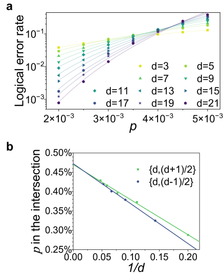
Figure 8: (a) Logical error rates $P_{L}$ of the triangular color code under the circuit-level noise model for various code distances $d$. The curves are fitted by the ansatz $P_{L}=\alpha p^{\beta}$, where $\alpha$ and $\beta$ vary with $d$. (b) The intersections of pairs of curves of $P_{L}$ with distances $\{d,(d+1)/2\}$ and $\{d,(d-1)/2\}$. From the linear extrapolation of the data, the threshold is around $0.47\%$.

IV.1 Decoding algorithm

Let us clarify our decoding strategy in a specific example of Fig. 2b, where two-qubit logical operators $X_{L}\otimes X_{L}$ and $Z_{L}\otimes Z_{L}$ are measured in parallel. Suppose the logical qubits are in the PBC model with continuous measurements, $d$ rounds QEC circuits will be implemented alternately in the merged and split lattice. In the QEC circuits, we continue to use CNOT schedules of 6-weight stabilizers and give 8-weight and 4-weight CNOT schedules in Fig. 6, which meets the criterion proposed in Sec III.1.

At the beginning and end of the merged step, the Bell pairs are prepared and measured by the circuits in Fig. 5 and Fig. 9. Note that there are enough syndrome qubits with our qubit layout to act as ancilla in these two circuits, since the number of syndrome qubits is approximately $2n_{f}$ and the number of Bell states is approximately $n_{f}$, where $n_{f}$ is the number of the faces in the middle region. Remarkably, after measuring Bell state measurements, the 8-weight stabilizers will become 4-weight stabilizers in the next QEC round. Therefore, in the $(3d+3)/2$ layer, the syndromes of the green or blue stabilizers in the connection part that used to be 8-weight stabilizers in the $(3d+1)/2$ layer need to be multiplied by the outcomes of two Bell pair measurements.

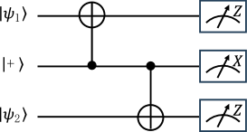
Figure 9: Circuit to measure $X\otimes X$ and $Z\otimes Z$ using a $\ket{+}$ state as ancilla. The result of $X\otimes X$ is the measurement outcome on $\ket{+}$, and the result of $Z\otimes Z$ is the product of measurement outcomes on $\ket{\psi_{1}}$ and $\ket{\psi_{2}}$. After the measurements, all the states will be discarded. Note that this circuit can be viewed as the inverse of the circuit in Fig 5

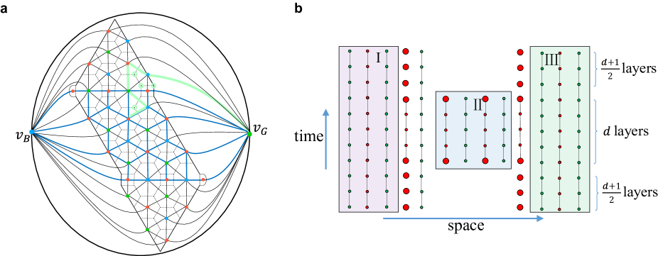
Figure 10: (a) The merged dual lattice $\mathcal{L}^{m}$ of lattice surgery of color code lattice surgery for measuring $X_{L}\otimes X_{L}$ and $Z_{L}\otimes Z_{L}$ in parallel. The lattice is divided into several subareas by the blue lines. An example of the path that ends inside the lattice and corresponding correction are illustrated by green lines and circles. (b) Vertices in decoding graph $\mathcal{G}^{ls}_{RG}$ (or lattice $\mathcal{L}^{ls}_{C}$). Two dimensions in space are compressed into one. The boundary vertex $v_{G}$ is not shown, although it is also in each layer of $\mathcal{G}^{ls}_{RG}$ or $\mathcal{L}^{ls}_{C}$. In our simulation, regions i@ and iii@ are split in the first and last $(d+1)/2$ layers and merged by region ii@ in the middle $d$ layers. The magnified vertices represent red vertices in the boundary vertex set $\tilde{V}$. Beyond the three regions, the vertices in $V_{R}^{m}\cup V_{G}^{m}$ are retained in each layer of the split steps. To avoid clutter, only vertical edges are shown, while horizontal edges as well as diagonal edges in $\mathcal{G}^{ls}_{RG}$ or $\mathcal{L}^{ls}_{C}$ are omitted.

Before introducing the decoding algorithm, we specify some notions about lattices and vertices. We use $\mathcal{L}^{m}$ ($\mathcal{L}^{s}$), $\mathcal{L}^{m}_{C}$ ($\mathcal{L}^{s}_{C}$) and $\mathcal{L}^{ls}_{C}$ to denote 2-D merged (split) dual lattice, 2-D restricted merged (split) lattice and 3-D restricted lattice, respectively. In 3-D restricted lattice $\mathcal{L}^{ls}_{C}$, the vertices of $d$ layers in the middle are from merged lattice $\mathcal{L}^{m}_{C}$ and the vertices in other layers are from split lattice $\mathcal{L}^{s}_{C}$ (see Fig. 10). In particular, attention is paid to the red vertices in the lattice $\mathcal{L}^{m}$. The red vertices in region $k$ ($k=1,2,3$) forms a vertex set denoted by $V_{R}^{k}$. Beyond the three regions, there are some 2-weight, 4-weight or 8-weight stabilizers in the connection parts, corresponding to vertices in set $V_{K}^{m}$ ($K\in\{R,G,B\}$ representing colors). We also define a boundary vertex set in $\mathcal{L}^{ls}_{C}$: $\tilde{V}=\{v_{x}^{t}|v_{x}\in\{v_{B},v_{G}\}\cup V_{R}^{m},\,t=1,2,...,2d+1\}\cup\{v_{x}^{t}|v_{x}\in V_{R}^{2},t=(d+3)/2\,\,{\rm or}\,\,(3d+3)/2\}$.

There are two goals of the lattice surgery decoding algorithm. One is obtaining the correction set $R\subseteq F(\mathcal{L}^{m})$ as accurately as possible and the other is obtaining the correct measurement results of $X_{L}\otimes X_{L}$ and $Z_{L}\otimes Z_{L}$. Overall, our decoding strategy has three main parts. At the beginning, we construct three decoding graphs $\mathcal{G}_{C}$ ($C\in\{RG,RB,GB\}$) with $2d+1$ layers (see Fig. 10b). The edges and their weights in $\mathcal{G}_{C}$ can be obtained by simulating lattice surgery circuits by the automatic procedure in a similar method as it in Sec III.2. In the next step, we input the syndrome changes $\sigma$ and apply the MWPM algorithm. Likewise, we map the matching results to 3-D lattice $\mathcal{L}^{ls}_{C}$. Lastly, each path is projected on the 2-D merged dual lattice $\mathcal{L}^{m}$. There are three types of paths after projection. The first is enclosed and the second starts and ends with $v_{G}$ or $v_{B}$. These two types of paths can divide the lattice into two complementary regions and we select the smaller one as the correction. The third type is the path that starts or ends with the vertices in $V_{R}^{m}\cup V_{R}^{2}$ and not enclosed. This results from the indeterminate measurement results in $V_{R}^{m}$ and $V_{R}^{2}$, which lead to two open boundaries in the time direction. As illustrated in Fig. 10a, we divide lattice $\mathcal{L}^{m}$ into several subareas and find the smaller region separated by the path in each subarea as the correction. Note that the syndrome of the error suffusing any subareas is trivial up to the syndrome in $V_{R}^{m}\cup V_{R}^{2}$.

As mentioned, the measurement outcome of $X_{L}\otimes X_{L_{2}}$ (or $Z_{L_{1}}\otimes Z_{L_{2}}$) is also required to determine. We use the product of all measurement outcomes of the starred stabilizers in the $(d+3)/2$ layer as the raw result. Apparently, the raw result is inaccurate unless there are no error affecting the measurement results. Therefore, if any syndrome change of the starred stabilizer occurs before or in the $(d+3)/2$ layer, we flip the raw result. Besides, we specifically consider the third type of paths mentioned above. The syndrome of the correction $R_{s}$ obtained from the third type of paths and the actual syndrome change may be different in some boundary vertices from $V_{R}^{m}\cup V_{R}^{2}$. If such vertices are before or in the $(d+3)/2$ layer and the number of these vertices is odd, the raw result also needs to be flipped.

In summary, the decoding algorithm is applied as follows.

• Input $d$, $p$ and syndrome changes $\sigma$ and construct 2-D merged dual lattice $\mathcal{L}^{m}$. For $C\in\{RG,RB,GB\}$, construct 3-D restricted lattices $\mathcal{L}^{ls}_{C}$ and decoding graph $\mathcal{G}^{ls}_{C}$ by the automatic procedure in the similar way as before.

• For $C\in\{RG,RB,GB\}$, apply the MWPM algorithm on $\mathcal{G}^{ls}_{C}$ to pair up the vertices in $\sigma_{C}=\sigma\cap V(\mathcal{G}^{ls}_{C})$ and obtain a path set $S_{C}$.

• For path $s\in S_{C}$, check whether the edge $e\in E(\mathcal{G}^{ls}_{C})$ on $s$ satisfies $e\in E[\mathcal{L}^{ls}_{C}]$. If not, replace $e$ with the shortest path connecting endpoints of $e$ in $\mathcal{L}^{ls}_{C}$.

• Combine path sets $S=S_{RG}\cup S_{RB}\cup S_{GB}$. For $s_{1}$, $s_{2}$ in $S$, if $s_{1},s_{2}$ can be connected, replace $s_{1}$, $s_{2}$ of $S$ with their connection $s_{1}+s_{2}$. Repeat this operation until all the paths in $S$ cannot be connected.

• For path $s\in S$, projects $s$ to $\mathcal{L}^{m}$. If ${\rm proj}(s)$ divide $\mathcal{L}^{m}$ into two regions, select the smaller one as the correction. Otherwise, select the smaller region separated by ${\rm proj}(s)$ in each subarea as the correction $R_{s}$. Output the total correction set $R=\oplus_{s}R_{s}$.

• Initialize the measurement outcome of $X_{L}\otimes X_{L}$ (or $Z_{L}\otimes Z_{L}$) $m_{o}$ as the product of measurement results of the starred stabilizers in the $(d+3)/2$ layer. For path $s\in S$, if an odd number of syndrome changes of starred stabilizers in $s$ occurs before the $(d+3)/2+1$ layer, replace $m_{o}$ with $-m_{o}$. For $s$ that has an endpoint in $\{v_{x}^{t}|v_{x}\in V_{R}^{m}\cup V_{R}^{2},t\leq(d+3)/2\}$, compare the syndrome of correction $R_{s}$ in the lattice $\mathcal{L}^{m}$ and the projections of actual syndrome changes. If they differ in an odd number of vertices, replace $m_{o}$ with $-m_{o}$. Output $m_{o}$ as the measurement outcome.

IV.2 Numerical results and further discussions

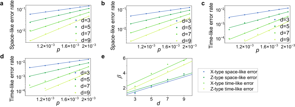
Figure 11: Space-like error rates and time-like error rates in the lattice surgery for various code distances $d$. All the curves are fitted by the ansatz $\alpha p^{\beta}$. (a-b) $X$-type and $Z$-type space-like errors. (c-d) $X$-type and $Z$-type time-like error rates. (e) Parameter $\beta$ of the curves in (a-d) for various code distances $d$. The parameters $\beta$ in space-like error rates and time-like error rates are fitted by $\beta=d/3+c_{1}$ and $\beta=d/2+c_{2}$ respectively.

We use the Monte Carlo simulation to test the performance of our algorithm. For the results in the simulations, we say a space-like error occurs if $R$ causes a logical error, and a time-like error occurs if $m_{o}$ is an incorrect outcome. The numerical results of the error rates of these two type of errors are shown in Fig. 11. The error rate curves are also fitted by the ansatz $\alpha p^{\beta}$. In principle, we estimate that the curves space-like error rates have the parameters $\beta\sim d/3$, since our decoding algorithm is based on the projector decoder, which admits that it can correct all the errors of weight at most $d/3$ (up to an additive constant) [32]. On the other hand, the time-like error curves are expected to have the parameters $\beta\sim d/2$, since they mainly result from the inaccurate measurement results of $d$ rounds of QEC circuits. Therefore, in Fig. 11e, we use the lines with fixed slopes to fit the parameters $\beta$ of the curves, which indicates that the space-like effective code distance is less than that the time-like one. Note that the rates of X-type and Z-type errors are not equal in our simulation, and we speculate that this is due to the order of the X-type and Z-type stabilizer measurements.

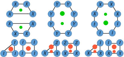
Figure 12: Vertices in $X$-type ($Z$-type is similar) decoding graphs of different stabilizers in the color code lattice surgery. The magnified points represent virtual vertices. If the corresponding stabilizer has $I$ or $Z$ terms in the top or bottom half, two vertices are located in a face, one of which is a virtual vertex. If a Y-type stabilizer occurs in a the decoding graph, the virtual vertex should be added since it cannot detect $Y$ errors. Two vertices in the same face are not connected and will be projected into the same position in the 2-D lattice.

The effectiveness of our decoding algorithm is demonstrated by the above numerical results in the example of $X_{L}\otimes X_{L}$ and $Z_{L}\otimes Z_{L}$ measurements. A natural question is whether the algorithm adapts to other situations in the lattice surgery. In fact, one only needs to modify the connection parts of each layer of the decoding graphs to guarantee the execution of the algorithm. Corresponding to different stabilizers in the color code lattice surgery, Fig. 12 shows the modifications of the vertices in the connection parts.

Specifically speaking, when we only perform $X_{L}\otimes X_{L}$ measurement, some 8-weight X-type stabilizers are divided into 4-weight stabilizers in the X-type decoding graph. At the same time, some 4-weight and 2-weight stabilizers are trivial ($I$ tensor products) in the Z-type decoding graph, so we added some virtual red vertices to hold the dual lattice three-colorable. Similar to space boundary vertices $v_{G}^{t}$ and $v_{B}^{t}$, such a virtual vertex does not carry any syndrome information but is just used for pairing up syndrome changes.

In Fig. 12, we also show the stabilizers when performing other types of color code lattice surgery in Ref [18, 38]. Some virtual vertices may be added, which results from the special forms of the stabilizers. A common vertex and a virtual vertex are located in a face if the corresponding stabilizer is trivial for the top or bottom half. For instance, the 8-weight $Y$ tensor product stabilizer can detect the $Z$ error and corresponds to a common vertex, while it cannot detect the $Y$ error so that we add a virtual vertex. These two vertices are not connected in the decoding graph, and will be projected in the same position in the 2-D lattice.

V State injection

In this section, we propose the state injection protocol of the triangular color code. First, we describe the process and the principles of the protocol in Sec V.1. We also prove that our protocol is optimal compared to the state injection protocol in any CSS code. In Sec V.2, the performances of diverse post-selection schemes are shown by numerical results.

V.1 State injection protocol

State injection is the process of obtaining an arbitrary logical state $\ket{\psi_{L}}$ from a physical state $\ket{\psi}$. Let us describe our state injection protocol of triangular color code. The protocol is executed in two steps. As illustrated in Fig. 13a, in the first step, the top qubit is initialized to $\ket{\psi}$ and the other qubits are initialized to Bell states $\ket{\phi}=\frac{1}{\sqrt{2}}(\ket{00}+\ket{11})$ in pairs. In the second step, the QEC cycles are performed with the CNOT schedule we give in Fig. 13b, which is carefully selected from 12 different schedules (see Appendix B for details).

To prove that the final state is $\ket{\psi_{L}}$ after all noiseless operations, one can simply verify the following equation:

$$\ket{\psi_{L}}\bra{\psi_{L}}\prod_{i}\frac{I+S_{i}}{2}\ket{\psi}\ket{\phi}^{\otimes m}$$ (2)

$$= \frac{I+\alpha X_{L}+\beta Y_{L}+\gamma Z_{L}}{2}\prod_{i}\frac{I+S_{i}}{2}\ket{\psi}\ket{\phi}^{\otimes m}$$

$$= (\prod_{i}\frac{I+S_{i}}{2})\frac{I+\alpha X_{L}+\beta Y_{L}+\gamma Z_{L}}{2}\ket{\psi}\ket{\phi}^{\otimes m}$$

$$= \prod_{i}\frac{I+S_{i}}{2}\ket{\psi}\ket{\phi}^{\otimes m},$$

where $(I+\alpha X+\beta Y+\gamma Z)/2=\ket{\psi}\bra{\psi}$ and $S_{i}$ is the stabilizer generator of the triangular color code. Hence, the final state $\prod_{i}(I+S_{i})/2\ket{\psi}\ket{\phi}^{\otimes m}$ is the $+1$ eigenstate of $\ket{\psi_{L}}\bra{\psi_{L}}$, i.e., $\prod_{i}(I+S_{i})/2\ket{\psi}\ket{\phi}^{\otimes m}=\ket{\psi_{L}}$.

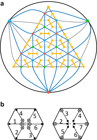
Figure 13: (a) Prime (dashed lines) and dual (solid lines) lattice of state injection protocol. The qubits are prepared in Bell pairs (yellow) except for the injected qubit on the top. The lattice is divided into several subareas by the blue lines. (b) The CNOT schedule in the state injection protocol that offers the optimal logical error rate.

The state injection protocol is non-fault-tolerant because a single error in the circuit may cause a logical error that cannot be corrected by the decoding algorithm. More seriously, some errors cannot even be detected, which means post-selection is also powerless against these errors. For example, the error occurring in the top qubit $\ket{\psi}$ before the first QEC cycle cannot be identified, since the injection protocol is applicable to an arbitrary state, even though it is a faulty state.

In our protocol, there are two types of errors that cannot be detected. The first is the single-qubit error when preparing the physical state $\ket{\psi}$. The second is the errors after some CNOT gates in the first QEC cycle, including $X\otimes I$, $Z\otimes Z$ and $Y\otimes Z$ errors after the CNOT gate between $\ket{\psi}$ and syndrome qubit $\ket{+}$, and $X\otimes X$ error after the CNOT gate between $\ket{\psi}$ and syndrome qubit $\ket{0}$.

Therefore, with the post-selection, the logical error rates of our state injection protocol is

$$P_{L}=\frac{4}{15}p_{2}+p_{I}+\frac{2}{3}p_{1}+\mathcal{O}(p^{2}),$$ (3)

where $p_{2}$ is the error rate of CNOT gates, and $p_{I}+2/3p_{1}$ is the error rate of preparing $\ket{\psi}$, which is consistent with Ref [29] and [30]. Here we assume that $\ket{\psi}$ initialization is performed one time step before the first CNOT gate on $\ket{\psi}$ is applied. Hence there is no need to consider the contribution of idle errors of $\ket{\psi}$ to $P_{L}$.

Compared to previous works in surface codes, our protocol admits a lower logical error rate (see second column in Table. 1). Further, we claim that our protocol is optimal among all state injection protocols in CSS code. Let us clarify it clearly with the following theorem.

Theorem 1

For any CSS code with standard stabilizer measurement circuits, the lower bound of the logical error rate of a state injection protocol is ${4}/{15}p_{2}+p_{I}+{2}/{3}p_{1}+\mathcal{O}(p^{2})$ under the circuit-level depolarizing noise model.

Here standard stabilizer measurement circuits are the circuits using CNOT gates, measurement in $Z$- (or $X$-) basis and $\ket{0}$ (or $\ket{+}$) as ancilla for Z-type (or X-type) stabilizer measurements. Now let us prove the theorem by stating that several errors must not be detected in the state injection circuits. Without loss of generality, we suppose that $\ket{\psi}$ first couples with syndrome qubit $\ket{+}$ and then couples with syndrome qubit $\ket{0}$ in a QEC cycle. An obvious fact is that any error of $\ket{\psi}$ before the first stabilizer measurement is undetectable since $\ket{\psi}$ is arbitrary for an injection protocol. Therefore, the error of $\ket{\psi}$ initialization cannot be detected with rate $p_{I}+{2}/{3}p_{1}+\mathcal{O}(p^{2})$. Besides, the $X$ error of $\ket{\psi}$ before the first CNOT gate between $\ket{\psi}$ and $\ket{0}$ but after the first CNOT between $\ket{+}$ and $\ket{\psi}$ is undetectable with the error rate of at least $p_{2}/15+\mathcal{O}(p^{2})$ , in which case the error is exactly $I\otimes X$ error after the first CNOT gate between $\ket{\psi}$ and $\ket{+}$. Further, utilizing the commuting relationship, a $Z\otimes Z$ error after the first CNOT gate between $\ket{+}$ and $\ket{\psi}$ is equivalent to an $I\otimes Z$ error before the stabilizer measurement, which is undetectable. Likewise, an $X\otimes X$ error after the first CNOT gale between $\ket{\psi}$ and $\ket{0}$ is also undetectable. Lastly, since $I\otimes X$ and $Z\otimes Z$ are undetectable, their product $Z\otimes Y$ after the first CNOT gate is also undetectable. In total, the logical error rate in a state injection protocol is at least ${4}/{15}p_{2}+p_{I}+{2}/{3}p_{1}+\mathcal{O}(p^{2})$, which is exactly the result in our protocol. Hence, we prove that our protocol is the optimal one among all state injection protocols in CSS codes.

V.2 Post-selection schemes and numerical results

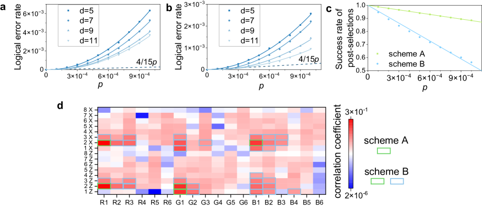
Figure 14: (a-b) The logical error rates of the state injection protocol in schemes A and B respectively, where the preparation of the injected state is assumed to be noiseless since it always causes a logical error. (c) Success rates of the post-selection as the linear function of the physical error rate $p$. The data are obtained from the state injection with $d=11$, since the results with other code distances are very close to them. (d) Correlation coefficients between syndrome changes and the occurrence of logical errors. The label, say R2 and 3Z, means the syndrome of the second red $Z$-type stabilizer (in the order from top to bottom and left to right in Fig. 13a) in the third QEC round. The post-selected syndromes in schemes A and B are framed.

Injection protocol	Logical error rate	Success rate of post-selection	Other features
on planar surface codes [29]	$\frac{2}{5}p_{2}+2p_{I}+\frac{2}{3}p_{1}+\mathcal{O}(p^{2})$	$60\%$ with $p=10^{-3}$	two steps where physical state is first injected to a $d=7$ logical qubit
on rotated surface codes from corner [30]	$\frac{3}{5}p_{2}+2p_{I}+\frac{2}{3}p_{1}+\mathcal{O}(p^{2})$	no data	only gives results of $d\leq 5$
on rotated surface codes from middle [30]	$\frac{3}{5}p_{2}+p_{I}+\frac{2}{3}p_{1}+\mathcal{O}(p^{2})$	no data	only gives results of $d\leq 5$
on triangular color codes	$\frac{4}{15}p_{2}+p_{I}+\frac{2}{3}p_{1}+\mathcal{O}(p^{2})$	around $98\%$ with $p=10^{-4}$ and $88\%$ with $p=10^{-3}$	one step to the logical qubit with any large code distance

Table 1: Comparison of several state injection protocols

In the last section, we theoretically analyze the leading order term of the logical error rate in our protocol. In this section, we show the details of the post-selection schemes and estimate the logical error rates in diverse schemes by numerical simulations. In our simulations, the noise model in Sec II.4 continues to be used in the QEC circuits and the Bell state initialization circuits. We also assume that the initialization of $\ket{\psi}$ is perfect, since errors in this step always cause logical errors. The logic error rates are counted after $d+1$ rounds of QEC circuits.

Although the state injection protocol is non-fault-tolerant, it still requires decoding to suppress errors. We mainly follow the decoding strategy in Sec III.2 but make three minor changes. First, in the 1st step when constructing the decoding graphs, we take the errors in the Bell state initialization circuits into account. Second, the definition of boundary vertex set $\tilde{V}$ is modified as $\{v_{x}^{t}|v_{x}\in\{v_{R},v_{B},v_{G}\},t=1,2,...,d+1\,\,{\rm or}\,\,v_{x}\,\,{\rm{is\,\,red}\,\,and}\,\,t=1\}$. This means that the red vertices in the first time layer are boundary vertices because the outcomes of the stabilizer measurements in these positions are undetermined. Third, in the 5th step, the path $s$ may start or end with red vertex in the first time layer, whose projection cannot divide $\mathcal{L}^{*}$ into two parts. In this case, we use the method similar to that in Sec IV.1 to divide $\mathcal{L}^{*}$ into several subareas to address this problem (see Fig. 13a).

In order to further suppress the logical error rate $P_{L}$, post-selection schemes are introduced. The post-selection means that if some syndromes are not as expected, we discard current states and restart the state injection protocol. Our results show that the post-selections only need to be applied to five syndromes to minimize the leading order term of $P_{L}$ (see scheme A in Fig. 14). By simulating the perfect circuit added by the single error in different positions, we find that there are 90 types of single errors will lead to a logical error with the probability of $12.4p+\mathcal{O}(p^{2})$, and 86 of them can be detected by those five syndromes. The numerical results show that the logical error rate of post-selection scheme A is close to $4/15p$ when $p=10^{-4}$ (see Fig. 14a).

When $p=10^{-3}$, however, the logical error rate is more than a dozen times of $4/15p$, since higher order terms contribute a lot in this case. Therefore, it is necessary to apply post-selection to more syndromes to suppress higher-order errors. To understand which syndromes are related to logical errors, we test the correlation coefficients of syndrome changes and the occurrence of logical errors by the Monte Carlo simulations in a $d=7$ triangular color code with $p=10^{-3}$ (see Fig. 14d). The correlation coefficient of events $A$ and $B$ is computed by

$$\rho_{AB}=\frac{|p(AB)-p(A)p(B)|}{\sqrt{p(A)(1-p(A))p(B)(1-p(B))}},$$ (4)

where $p(A)$, $p(B)$, $p(AB)$ are the probabilities of $A$, $B$, both $A$ and $B$ occurring respectively.

According to these correlation coefficients, one can design the post-selection scheme flexibly with the syndromes whose correlation coefficients are larger. Apparently, the post-selection with more syndromes will lead to lower success rate of post-selection. Here we present an example (scheme B in Fig. 14) where the logical error rate is reduced by 4 times when $p=10^{-3}$ compared to scheme A, while the success rate of post-selection is still over $56\%$.

Contrary to previous works on state injections in surface codes, the success rate of post selections in our protocol does not decay sharply as the code distance increases, but is only linearly related to the physical error rate (see Fig. 14c and Table. 1). On account of the fact that errors farther from the top qubit $\ket{\psi}$ are on a longer logical string (i.e., the data qubit string that connects left and right boundaries), the stabilizers of the post-selected syndromes are located around the top qubit. Therefore, the number of post-selected syndromes does not increase with the code distance, which means one can inject a physical state into a logical state with arbitrary code distance in one step, rather than two steps as in Ref [29]. In addition, this feature provides our protocol with a high success rate of post-selection, around $98\%$ ($88\%$) in scheme A when $p=10^{-4}$ ($10^{-3}$).

VI Conclusion and outlook

In this paper, we solved several problems in the road towards practical fault-tolerant quantum computation with 2-D color codes, including improving the threshold of the triangular color code, decoding color code lattice surgery under circuit-level noise and proposing an optimal state injection protocol. We believe these works are expected to promote the development of quantum computing based on color codes.

There are still many challenges left for future work. For example, the PBC model mentioned in the main text is probably not the final form of quantum computation based on color codes, since it does not utilize the advantages of transversal Clifford gates on color codes. According to the specific quantum algorithm, a proper way to use color codes for quantum computing still needs to be developed.

In addition, we also notice the color codes with other boundaries, such as square color codes or thin color codes [38, 18], which are also the candidates for the color code quantum computing. These color codes encode more than one logical qubit in an individual patch and may reduce the overhead further under the special structured noise (e.g., biased noise). We do not perceive any fundamental difficulties in applying our lattice surgery decoding strategies to them. In particular, thin color codes with $d_{z}>d_{x}$ can reduce the cost of magic state distillation, since the distillation error is more sensitive to the Z-type error [28]. Based on the feature of parallel measurements and our lattice surgery decoding algorithm, estimating and optimizing the time and space overhead of magic state distillation in a color-code-based quantum computation will be an interesting question.

Lastly, recent work [49] demonstrates that the local connectivity of surface codes can be reduced from four to three by time-dynamics. An open question is whether the similar technique can be used to relax the high hardware requirement of high-weight stabilizer measurements in color codes.

Appendix A Automatic procedure for constructing decoding graphs

The automatic procedure extracts error information of noisy circuits based on the circuit-level depolarizing noise model. In a noisy quantum circuit, we approximate every noisy operation by an ideal operation followed by the depolarizing error channel $\mathcal{E}_{1}$ or $\mathcal{E}_{2}$.

As mentioned in the main text, in each time, the automatic procedure simulates an ideal QEC circuit attached to a single error in the different channels in the circuit. If the error is located in channel $\mathcal{E}_{1}$, the error is $X$, $Y$ or $Z$. If the error is located in channel $\mathcal{E}_{2}$, the error is one of $P_{1}\otimes P_{2}$ where $P_{1},P_{2}\in{I,X,Y,Z}$ and $P_{1}\otimes P_{2}\neq I\otimes I$.

In fact, there is no need to simulate every round of the QEC cycle, since the noisy QEC circuits simply repeat $d$ times in addition to a perfect QEC round. For each position and type of error, we only simulate the circuit in two QEC rounds, where the error is only added in the first round and the circuit in the second round is perfect. We record the vertex sets corresponding to the syndrome changes in each simulation.

In the automatic procedure, we connect the syndrome changes in pairs to form edges by the following rule. First, we connect the vertices that project into the same position, if they exist. Then we connect the remaining vertices with the same color, if they exist. Using the well-designed CNOT schedules in Fig. 6, there are at most two vertices unmatched in one decoding graph after this step. If there are two vertices left, we connect them and if there is only one vertex left, we check the syndrome of the error and connect the vertex with the proper boundary vertex.

Based on these connections, the edges in the first two layers of $\mathcal{G}_{C}$ are determined, notated by $e_{0}=(v_{1}^{t_{1}},v_{2}^{t_{2}})$. All edges $e_{0}$ obtained from the simulations in two QEC rounds form an edge set $\beta_{0}$. Then one can construct the edge set $\beta$ in $\mathcal{G}_{C}$ by $\beta_{0}$:

$$\beta=\{e=(v_{1}^{t_{1}},v_{2}^{t_{2}})|v_{1}^{t_{1}},v_{2}^{t_{2}}\in\mathcal{G}_{C},e//e_{0},e_{0}\in\beta_{0}\},$$ (5)

where we say two edges $e_{1}=(v_{1}^{t_{1}},v_{2}^{t_{2}})$, $e_{2}=(v_{3}^{t_{3}},v_{4}^{t_{4}})$ are parallel in a 3-D lattice if they have the same vertical projection and $t_{3}-t_{1}=t_{4}-t_{2}$, notated by $e_{1}//e_{2}$.

Suppose edge $e_{0}\in\beta_{0}$ is obtained from the syndrome changes of the single error $\epsilon$, the error rate corresponding to $e_{0}$ is $p_{\epsilon}(e_{0})$, where $p_{\epsilon}(e_{0})=p/3$ if ${\epsilon}$ is located in $\mathcal{E}_{1}$, otherwise $p_{\epsilon}(e_{0})=p/15$. By accumulating $p_{\epsilon}(e_{0})$ with different $\epsilon$, we obtained the error-rate-related weight of the edge $e=(v_{1}^{t_{1}},v_{2}^{t_{2}})\in\beta$:

$$w_{e}=\left\{\begin{aligned} &-\log\sum_{\begin{subarray}{c}e_{0}\in\beta_{0}^{(1)},\\ {\rm and}\,\,e_{0}//e\end{subarray}}\sum_{{\epsilon}}p_{\epsilon}(e_{0}),\quad{\rm if}\quad t_{1}=t_{2}=1,\\ &-\log\sum_{\begin{subarray}{c}e_{0}\in\beta_{0}^{(2)},\\ {\rm and}\,\,e_{0}//e\end{subarray}}\sum_{{\epsilon}}p_{\epsilon}(e_{0}),\quad{\rm if}\quad t_{1}=t_{2}=d+1,\\ &-\log\sum_{\begin{subarray}{c}e_{0}\in\beta_{0},\\ {\rm and}\,\,e_{0}//e\end{subarray}}\sum_{{\epsilon}}p_{\epsilon}(e_{0}),\quad\quad{\rm otherwise},\end{aligned}\right.$$ (6)

where $\beta_{0}^{(1)}=\{e_{0}|e_{0}=(v_{i}^{1},v_{j}^{1})\in\beta_{0}\}$ and $\beta_{0}^{(2)}=\{e_{0}|e_{0}=(v_{i}^{2},v_{j}^{2})\in\beta_{0}\}$. Note that the edges in the time boundaries (i.e., the first and last layers) are considered individually in the first two cases.

Appendix B Different CNOT schedules in the state injection protocol

In order to find the optimal CNOT schedule of state injection, we test 12 kinds of CNOT schedules as shown in Fig. 15. Note that $0^{+}$ is the CNOT schedule used in color code QEC circuits and other schedules are obtained by flipping or rotating $0^{+}$. We use these CNOT schedules since the flip or rotation operation will hold the relationship in the criterion of a proper CNOT schedule. The complete data of logical error rates to the leading order are shown in Table. 2.

Figure 15: Details of the 12 types of CNOT schedules we considered in the state injection. (a-l) correspond to $0^{+}$,$0^{-}$,$1^{+}$, …, $5^{-}$, respectively. The CNOT schedules with $+$ are obtained by rotating $0^{+}$, and CNOT schedule $k^{-}$ is the flip of $k^{+}$.

Table 2: Logical error rates in different CNOT schedules with and without post-selection

CNOT schedule	$P_{L}$ with post-selection (to the leading order)	$P_{L}$ without post-selection (to the leading order)
$0^{+}$	$0.6p$	$10.6p$
$0^{-}$	$1.2\dot{6}p$	$13.2\dot{6}p$
$1^{+}$	$0.\dot{3}p$	$9.8\dot{6}p$
$1^{-}$	$0.5\dot{3}p$	$11.1\dot{3}p$
$2^{+}$	$0.\dot{3}p$	$10.8p$
$2^{-}$	$0.2\dot{6}p$	$12.4p$
$3^{+}$	$0.6p$	$11.5\dot{3}p$
$3^{-}$	$1.2\dot{6}p$	$12.2p$
$4^{+}$	$1.2p$	$12.0\dot{6}p$
$4^{-}$	$p$	$12.\dot{6}p$
$5^{+}$	$0.9\dot{3}p$	$13.6p$
$5^{-}$	$p$	$11.7\dot{3}p$

Appendix C Other details of the simulations

We use Monte Carlo simulation to estimate the logical error rates in different cases. In each time of simulation, QEC circuits are executed for $d+1$ rounds in the color code decoding and state injection, and $2d+1$ rounds (including the merged step and split step) in the lattice surgery. In both three situations, the circuit in the last round is assumed to be noiseless.

Another key question is how to determine if there is a logical error after decoding. In the color code decoding, we check whether the product of correction $R$ and actual error $\epsilon$ is a logical operator (up to a stabilizer) by commutation relations.

In the lattice surgery, space-like and time-like errors should be considered separately. Note that the space-like logical error must anticommute with an odd number of starred stabilizers. The output correction $R$ may cause a logical error as well as the stabilizers of several Bell states in the middle region, since some boundary vertices are located inside the lattice. These stabilizers are trivial for our decoding, because they always anti-commute with an even number of starred stabilizers. The space-like errors in the top and bottom logical qubits are equivalent since $X_{L}\otimes X_{L}$ and $Z_{L}\otimes Z_{L}$ have been measured. For the time-like error, we set all the red boundary vertices with the initial syndromes $+1$ to guarantee that the expected outcome of $X_{L}\otimes X_{L}$ or $Z_{L}\otimes Z_{L}$ measurement is $+1$. Then we check the actual outcome to determine if there is a time-like logical error.

In the state injection, the correction $R$ may differ from the actual error $\epsilon$ by $X\otimes X$ (or $Z\otimes Z$) error in the qubits of the initial Bell pairs whose syndrome corresponds to two red vertices, since the measurements of red stabilizers do not have determined initial syndromes. However, they will be determined fault-tolerantly after sufficient rounds of measurements and then $X\otimes X$ will be corrected. Therefore, we do not think the decoding fails when such errors are left after decoding. From another perspective, such $X\otimes X$ (or $Z\otimes Z$) errors will not change the measurement result of the logical Pauli operators ($X_{L}$, $Y_{L}$ or $Z_{L}$) since the Bell pairs and the logical Pauli operator always have an even number of common qubits.

Lastly, we list the simulation times of the numerical results in the main text. In Fig. 8a and Fig. 11, each point is obtained by over $10^{6}$ simulations. In Fig. 14a and Fig. 14b, we obtain each point by $10^{3}/p$ times of simulations, where $p$ is the physical error rate ranging from $10^{-4}$ to $10^{-3}$.

References

- [1] Peter W Shor. Polynomial-time algorithms for prime factorization and discrete logarithms on a quantum computer. SIAM review, 41(2):303–332, 1999.
- [2] Richard P Feynman. Quantum mechanical computers. Optics news, 11(2):11–20, 1985.
- [3] Michael H Freedman, Alexei Kitaev, and Zhenghan Wang. Simulation of topological field theories by quantum computers. Communications in Mathematical Physics, 227(3):587–603, 2002.
- [4] John Preskill. Reliable quantum computers. Proceedings of the Royal Society of London. Series A: Mathematical, Physical and Engineering Sciences, 454(1969):385–410, 1998.
- [5] Michael A Nielsen and Isaac L Chuang. Quantum computation and quantum information. Cambridge university press, 2010.
- [6] Barbara M Terhal. Quantum error correction for quantum memories. Reviews of Modern Physics, 87(2):307, 2015.
- [7] Daniel Gottesman. Stabilizer codes and quantum error correction. California Institute of Technology, 1997.
- [8] Eric Dennis, Alexei Kitaev, Andrew Landahl, and John Preskill. Topological quantum memory. Journal of Mathematical Physics, 43(9):4452–4505, 2002.
- [9] Jiannis K Pachos. Introduction to topological quantum computation. Cambridge University Press, 2012.
- [10] Hector Bombin and Miguel Angel Martin-Delgado. Topological quantum distillation. Physical review letters, 97(18):180501, 2006.
- [11] Aleksander Marek Kubica. The ABCs of the color code: A study of topological quantum codes as toy models for fault-tolerant quantum computation and quantum phases of matter. PhD thesis, California Institute of Technology, 2018.
- [12] Austin G Fowler, Matteo Mariantoni, John M Martinis, and Andrew N Cleland. Surface codes: Towards practical large-scale quantum computation. Physical Review A, 86(3):032324, 2012.
- [13] Andrew J Landahl and Ciaran Ryan-Anderson. Quantum computing by color-code lattice surgery. arXiv preprint arXiv:1407.5103, 2014.
- [14] Christopher Chamberland, Aleksander Kubica, Theodore J Yoder, and Guanyu Zhu. Triangular color codes on trivalent graphs with flag qubits. New Journal of Physics, 22(2):023019, 2020.
- [15] Austin G Fowler, Adam C Whiteside, and Lloyd CL Hollenberg. Towards practical classical processing for the surface code. Physical review letters, 108(18):180501, 2012.
- [16] Ashley M Stephens. Fault-tolerant thresholds for quantum error correction with the surface code. Physical Review A, 89(2):022321, 2014.
- [17] Clare Horsman, Austin G Fowler, Simon Devitt, and Rodney Van Meter. Surface code quantum computing by lattice surgery. New Journal of Physics, 14(12):123011, 2012.
- [18] Felix Thomsen, Markus S Kesselring, Stephen D Bartlett, and Benjamin J Brown. Low-overhead quantum computing with the color code. arXiv preprint arXiv:2201.07806, 2022.
- [19] Daniel Litinski and Felix von Oppen. Lattice surgery with a twist: simplifying clifford gates of surface codes. Quantum, 2:62, 2018.
- [20] Daniel Litinski. A game of surface codes: Large-scale quantum computing with lattice surgery. Quantum, 3:128, 2019.
- [21] Austin G Fowler and Craig Gidney. Low overhead quantum computation using lattice surgery. arXiv preprint arXiv:1808.06709, 2018.
- [22] Christopher Chamberland and Earl T Campbell. Circuit-level protocol and analysis for twist-based lattice surgery. Physical Review Research, 4(2):023090, 2022.
- [23] Craig Gidney. Inplace access to the surface code y basis. arXiv preprint arXiv:2302.07395, 2023.
- [24] Christopher Chamberland and Earl T Campbell. Universal quantum computing with twist-free and temporally encoded lattice surgery. PRX Quantum, 3(1):010331, 2022.
- [25] Sergey Bravyi and Alexei Kitaev. Universal quantum computation with ideal clifford gates and noisy ancillas. Physical Review A, 71(2):022316, 2005.
- [26] Sergey Bravyi and Jeongwan Haah. Magic-state distillation with low overhead. Physical Review A, 86(5):052329, 2012.
- [27] Earl T Campbell and Mark Howard. Unified framework for magic state distillation and multiqubit gate synthesis with reduced resource cost. Physical Review A, 95(2):022316, 2017.
- [28] Daniel Litinski. Magic state distillation: Not as costly as you think. Quantum, 3:205, 2019.
- [29] Ying Li. A magic state’s fidelity can be superior to the operations that created it. New Journal of Physics, 17(2):023037, 2015.
- [30] Lingling Lao and Ben Criger. Magic state injection on the rotated surface code. In Proceedings of the 19th ACM International Conference on Computing Frontiers, pages 113–120, 2022.
- [31] Shraddha Singh, Andrew S Darmawan, Benjamin J Brown, and Shruti Puri. High-fidelity magic-state preparation with a biased-noise architecture. Physical Review A, 105(5):052410, 2022.
- [32] Michael E Beverland, Aleksander Kubica, and Krysta M Svore. Cost of universality: A comparative study of the overhead of state distillation and code switching with color codes. PRX Quantum, 2(2):020341, 2021.
- [33] Nicolas Delfosse. Decoding color codes by projection onto surface codes. Physical Review A, 89(1):012317, 2014.
- [34] Jack Edmonds. Paths, trees, and flowers. Canadian Journal of mathematics, 17:449–467, 1965.
- [35] Oscar Higgott. Pymatching: A python package for decoding quantum codes with minimum-weight perfect matching. ACM Transactions on Quantum Computing, 3(3):1–16, 2022.
- [36] A Robert Calderbank and Peter W Shor. Good quantum error-correcting codes exist. Physical Review A, 54(2):1098, 1996.
- [37] Andrew Steane. Multiple-particle interference and quantum error correction. Proceedings of the Royal Society of London. Series A: Mathematical, Physical and Engineering Sciences, 452(1954):2551–2577, 1996.
- [38] Markus S Kesselring, Julio C Magdalena de la Fuente, Felix Thomsen, Jens Eisert, Stephen D Bartlett, and Benjamin J Brown. Anyon condensation and the color code. arXiv preprint arXiv:2212.00042, 2022.
- [39] Sergey Bravyi, Graeme Smith, and John A Smolin. Trading classical and quantum computational resources. Physical Review X, 6(2):021043, 2016.
- [40] Austin G Fowler. Time-optimal quantum computation. arXiv preprint arXiv:1210.4626, 2012.
- [41] Bryan Eastin and Emanuel Knill. Restrictions on transversal encoded quantum gate sets. Physical review letters, 102(11):110502, 2009.
- [42] Robert Raussendorf, Jim Harrington, and Kovid Goyal. A fault-tolerant one-way quantum computer. Annals of physics, 321(9):2242–2270, 2006.
- [43] Tomas Jochym-O’Connor and Stephen D Bartlett. Stacked codes: Universal fault-tolerant quantum computation in a two-dimensional layout. Physical Review A, 93(2):022323, 2016.
- [44] Benjamin J Brown. A fault-tolerant non-clifford gate for the surface code in two dimensions. Science advances, 6(21):eaay4929, 2020.
- [45] Christopher Chamberland and Andrew W Cross. Fault-tolerant magic state preparation with flag qubits. Quantum, 3:143, 2019.
- [46] Christopher Chamberland and Kyungjoo Noh. Very low overhead fault-tolerant magic state preparation using redundant ancilla encoding and flag qubits. npj Quantum Information, 6(1):91, 2020.
- [47] Stergios Koutsioumpas, Darren Banfield, and Alastair Kay. The smallest code with transversal t. arXiv preprint arXiv:2210.14066, 2022.
- [48] David S Wang, Austin G Fowler, and Lloyd CL Hollenberg. Surface code quantum computing with error rates over 1%. Physical Review A, 83(2):020302, 2011.
- [49] Matt McEwen, Dave Bacon, and Craig Gidney. Relaxing hardware requirements for surface code circuits using time-dynamics. arXiv preprint arXiv:2302.02192, 2023.