SIM-Sync: From Certifiably Optimal Synchronization over the 3D Similarity Group to Scene Reconstruction with Learned Depth

Abstract

We present SIM-Sync, a certifiably optimal algorithm that estimates camera trajectory and 3D scene structure directly from multiview image keypoints. SIM-Sync fills the gap between pose graph optimization and bundle adjustment; the former admits efficient global optimization but requires relative pose measurements and the latter directly consumes image keypoints but is difficult to optimize globally (due to camera projective geometry).

The bridge to this gap is a pretrained depth prediction network. Given a graph with nodes representing monocular images taken at unknown camera poses and edges containing pairwise image keypoint correspondences, SIM-Sync first uses a pretrained depth prediction network to lift the 2D keypoints into 3D scaled point clouds, where the scaling of the per-image point cloud is unknown due to the scale ambiguity in monocular depth prediction. SIM-Sync then seeks to synchronize jointly the unknown camera poses and scaling factors (i.e., over the 3D similarity group) by minimizing the sum of the Euclidean distances between edge-wise scaled point clouds. The SIM-Sync formulation, despite nonconvex, allows designing an efficient certifiably optimal solver that is almost identical to the SE-Sync algorithm. Particularly, after solving the translations in closed-form, the remaining optimization over the rotations and scales can be written as a quadratically constrained quadratic program, for which we apply Shor’s semidefinite relaxation. We show how to add scale regularization in the semidefinite program to prevent contraction of the estimated scales.

We demonstrate the tightness, robustness, and practical usefulness of SIM-Sync in both simulated and real experiments. In simulation, we show (i) SIM-Sync compares favorably with SE-Sync in scale-free synchronization, and (ii) SIM-Sync can be used together with robust estimators to tolerate a high amount of outliers. In real experiments, we show (a) SIM-Sync achieves similar performance as Ceres on bundle adjustment datasets, and (b) SIM-Sync performs on par with ORB-SLAM3 on the TUM dataset with zero-shot depth prediction.

1 Introduction

3D scene reconstruction and camera trajectory estimation from image sequences remains one of the most fundamental and extensively studied problems in robotics and computer vision. At the heart of this problem lies (i) finding reliable feature correspondences, e.g., keypoints, across images (sometimes referred to as data association in robotics), and (ii) estimating camera poses given the associated features. In this paper, we focus on the camera trajectory estimation problem and denote $x_{i}=(R_{i},t_{i})\in\mathrm{SE}(3),i=1,\dots,N$ as the set of camera poses to be estimated.

A long list of formulations and solutions have been developed for camera trajectory estimation, for which we refer to [5, Chapter 9] and [29, Chapter 11]. We motivate our work by describing two of the most popular formulations.

The first formulation, exemplified by pose graph optimization (PGO) [24] for simultaneous localization and mapping (SLAM) in robotics, first estimates relative camera poses from image features, i.e., estimating $\tilde{x}_{ij}\approx x_{i}^{-1}x_{j}$ for $(i,j)\in{\cal E}$ with overlapping image features, and then solves an optimization problem that synchronizes $\{x_{i}\}_{i=1}^{N}$ from the relative measurements $\{\tilde{x}_{ij}\}_{(i,j)\in{\cal E}}$. The synchronization problem, despite nonconvex, has an objective function that is polynomial in the unknowns. Consequently, the seminal work SE-Sync [24, 9, 10] demonstrated efficiently solving the problem to certifiable global optimality using semidefinite programming (SDP) relaxations and customized low-rank SDP solvers. Holmes and Barfoot [14] derived similar SDP-based global optimality certificates for landmark-based SLAM, as long as the landmark measurements are in 3D, which preserves the polynomiality of the objective function.

The second formulation, exemplified by bundle adjustment (BA) [1, 25] for structure from motion (SfM) in computer vision, solves an optimization problem that jointly estimates camera poses and 3D keypoints by minimizing geometric reprojection errors. The key challenge to solve this formulation is that the objective function is no longer polynomial in the camera poses and 3D keypoints, but rather a sum of rational functions. Therefore, the most popular solution methods, e.g., COLMAP [1], Ceres [2], and GTSAM [12], rely on gradient-based local optimization techniques and can be sensitive to the quality of initialization. It is, however, not impossible to solve this formulation to global optimality. For example, by replacing the geometric reprojection error with the object space error, [26] recovers polynomiality and designed a globally convergent algorithm, albeit not based on SDP relaxations. It may also be possible to apply the SDP relaxation hierarchy designed for rational function optimization [7] to the BA formulation. However, the SDP relaxation hierarchy in [7] scales poorly (and worse than its polynomial counterpart) and such an attempt has never been made in the literature.

In summary, given image feature correspondences, the BA-type formulation estimates camera poses in a single step by minimizing an objective function that is directly constructed from image keypoints. The PGO-type formulation, however, takes a two-step approach, where the first step estimates relative camera poses and the second step performs pose synchronization. The BA-type formulation is more straightforward than the PGO-type formulation, but more difficult to optimize globally. Therefore, we ask the question: can we design a camera trajectory estimation formulation that (i) directly consumes image features and (ii) admits efficient global optimization?

Contributions. Inspired by the recent trend in computer vision [20, 17, 36, 21] that leverages a learned depth prediction network [23] for bundle adjustment, we propose a certifiably optimal camera trajectory estimation algorithm that directly consumes image feature correspondences. The key insight is that, with the help of a pretrained depth prediction network, 2D keypoint correspondences can be effectively lifted to 3D keypoint correspondences, leading to a formulation whose objective function is again polynomial in the unknown camera poses. Yet different from the formulation in multiple point cloud registration (MPCR) [11, 15], the lifted 3D keypoints have an unknown scaling factor (per camera frame) due to the scale ambiguity of depth prediction. As a result, our formulation seeks to estimate, for each camera frame $i\in[N]$, both the camera pose $(R_{i},t_{i})\in\mathrm{SE}(3)$ and the scaling factor $s_{i}>0$, i.e., an element $x_{i}=(s_{i},R_{i},t_{i})$ in the 3D similarity group $\mathrm{SIM}(3)$. For this reason, we call our formulation SIM-Sync, which performs synchronization over $\mathrm{SIM}(3)$ using pairwise image keypoint correspondences. A graphical illustration of SIM-Sync using the TUM dataset [28] as an example is provided in Fig. 1.

The nice property of our SIM-Sync formulation is that it allows designing a certifiably optimal solver in a way that is almost identical to SE-Sync. Specifically, we first solve the unknown translations as a function of the rotations and scales, arriving at an optimization problem whose objective is a quartic (i.e., degree-four) polynomial in the rotations and scales. Then, by creating scaled rotations $\widetilde{R}_{i}=s_{i}R_{i},i=1,\dots,N$, the quartic polynomial becomes quadratic and the problem becomes a quadratically constrained quadratic program (QCQP), for which we apply the standard Shor’s semidefinite relaxation [4]. Given the same number of camera frames $N$, our SIM-Sync relaxation leads to an SDP having the same matrix size as that of SE-Sync ($3N\times 3N$), but with fewer linear equality constraints (due to fewer quadratic equality constraints on $\widetilde{R}_{i}$). Moreover, we show that it is possible to regularize the scale estimation to be close to $1$ by adding $\sum_{i=1}^{N}(s_{i}^{2}-1)^{2}$ into the objective, which can be conveniently handled by the SDP relaxation with small positive semidefinite variables. This regularization effectively prevents contraction (i.e., $s_{i}$ tends to zero) of the estimated camera trajectory in certain test cases (e.g., the 3D grid graph).

We then conduct a suite of simulated and real experiments to investigate the empirical performance of SIM-Sync. Particularly, with simulations we show that (i) the SIM-Sync relaxation is almost always exact (tight) under small to medium noise corruption in the measurements, i.e., globally optimal estimates can be computed and certified; (ii) SIM-Sync achieves similar estimation accuracy as SE-Sync (and SE-Sync refined by g2o); (iii) SIM-Sync can be robustified against $40-80\%$ outlier correspondences by running GNC [33] and TEASER [34] to preprocess pairwise correspondences. With real experiments we show that (a) SIM-Sync compares favorably with Ceres on the BAL bundle adjustment dataset [1], and (b) SIM-Sync achieves similar performance as ORB-SLAM3 [8] on the TUM dataset [28] with zero-shot depth prediction.

Paper organization. We present the SIM-Sync formulation in Section 2, where we also derive the simplified QCQP formulation. We introduce the semidefinite relaxation and scale regularization in Section 3. We present experimental results in Section 4 and conclude in Section 5.

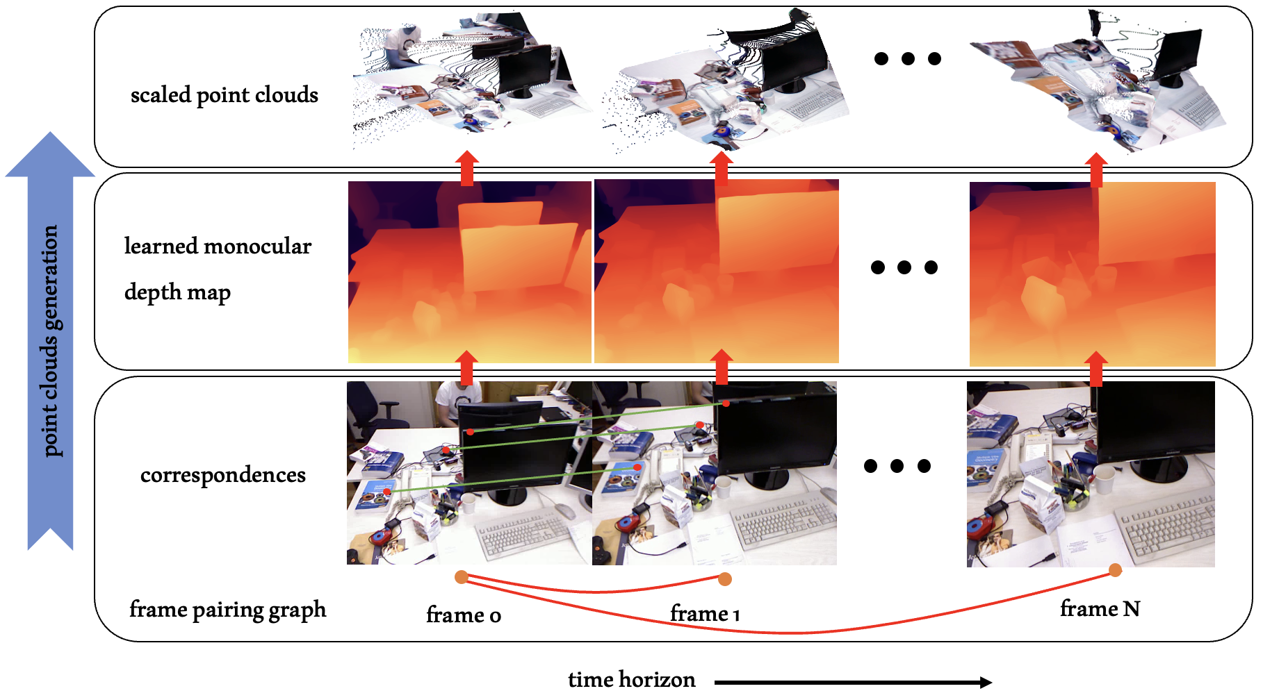
Figure 1: Illustration of SIM-Sync on the TUM dataset [28].

2 Problem Formulation

Consider a graph ${\cal G}=({\cal V},{\cal E})$, where each node $i\in{\cal V}=[N]$ is associated with an RGB image $I_{i}\in{{\mathbb{R}}^{H\times W\times 3}}$ and an unknown camera pose $(R_{i},t_{i})\in\mathrm{SE}(3)$, and each edge $(i,j)\in{\cal E}$ contains a set of $n_{ij}$ dense pixel-to-pixel correspondences ${\cal C}_{ij}=\{p_{i,k}\leftrightarrow p_{j,k}\}_{k=1}^{n_{ij}}$ with $p_{i,k}\in{{\mathbb{R}}^{2}}$ the $k$-th pixel location in image $I_{i}$ and $p_{j,k}\in{{\mathbb{R}}^{2}}$ the $k$-th pixel location in image $I_{j}$. Assuming all the camera intrinsics $\{K_{i}\}_{i=1}^{N}$ are known, we can compute

$$\widetilde{p}_{i,k}=K_{i}^{-1}\left[\begin{array}[]{c}p_{i,k}^{x}\\ p_{i,k}^{y}\\ 1\end{array}\right]$$ (4)

as the bearing vector normalized by the camera intrinsics. The third entry of $\widetilde{p}_{i,k}$ is equal to $1$.

Pretrained depth prediction. Suppose we are given a pretrained depth estimation network that, for each image $I_{i}$, produces a depth map. Let $d_{i,k}>0$ be the predicted depth of $p_{i,k}$ and $s_{i}>0$ be the unknown scale coefficient for image $I_{i}$. Consequently,

$$\widehat{p}_{i,k}=s_{i}d_{i,k}\widetilde{p}_{i,k}$$ (5)

corresponds to the 3D location of $p_{i,k}$ in the $i$-th camera frame. Effectively, with the pretrained depth predictor, for every $(i,j)\in{\cal E}$, we have a pair of scaled point cloud measurements $\{d_{i,k}\widetilde{p}_{i,k}\}_{k=1}^{n_{ij}}$ and $\{d_{j,k}\widetilde{p}_{j,k}\}_{k=1}^{n_{ij}}$, as shown in Fig. 1 top panel.

The SIM-Sync formulation. We are interested in estimating the unknown camera poses and the per-image scale coefficients $\{x_{i}=(s_{i},R_{i},t_{i})\}_{i=1}^{N}$. We formulate the following optimization

$$\min_{\begin{subarray}{c}s_{i}>0,R_{i}\in\mathrm{SO}(3),t_{i}\in{{\mathbb{R}}^{3}}\\ i=1,\dots,N\end{subarray}}\sum_{(i,j)\in{\cal E}}\sum_{k=1}^{n_{ij}}w_{ij,k}\left\lVert\left(R_{i}\underbrace{(s_{i}d_{i,k}\widetilde{p}_{i,k})}_{\widehat{p}_{i,k}}+t_{i}\right)-\left(R_{j}\underbrace{(s_{j}d_{j,k}\widetilde{p}_{j,k})}_{\widehat{p}_{j,k}}+t_{j}\right)\right\rVert^{2}$$ (SIM-Sync)

where the objective function seeks to minimize the 3D point-to-point distances because $(R_{i},t_{i})$ transforms $\widehat{p}_{i,k}$, and $(R_{j},t_{j})$ transforms $\widehat{p}_{j,k}$ into the same global coordinate frame. In (SIM-Sync), we include $w_{ij,k}>0$ for generality: these known weights capture the potential uncertainty of the correspondences. Usually these weights are unknown and in our experiments we use GNC and TEASER to estimate them so that $w_{ij,k}=1$ indicates inliers and $w_{ij,k}=0$ indicates outliers.

Anchoring. Problem (SIM-Sync) is ill-defined. One can choose $s_{i}\rightarrow 0,\forall i=1,\dots,N$, $t_{1}=t_{2}=\dots=t_{N}=\text{constant}$, and the objective of (SIM-Sync) can be set arbitrarily close to zero. To resolve this issue, we anchor the first frame and set $R_{1}={\mathbf{I}}_{3},t_{1}={\mathbf{0}},s_{1}=1$, which is common practice in many related pose graph estimation formulations [24].

2.1 A QCQP Formulation

The (SIM-Sync) formulation is readily in the form of a polynomial optimization problem (POP). The objective function is a quartic polynomial, the constraint $s_{i}>0$ is an affine polynomial inequality, and the constraint $R_{i}\in\mathrm{SO}(3)$ is equivalent to a set of quadratic polynomial constraints [32]. Therefore, one can directly apply Lasserre’s hierarchy of moment relaxations [18] to design convex SDP relaxations for (SIM-Sync). However, as noted in [32], a direct application of Lasserre’s hierarchy often leads to SDPs beyond the scalability of current solvers. Therefore, in the following we will simplify (SIM-Sync) as a quadratically constrained quadratic problem (QCQP), in a way that is inspired by SE-Sync [24].

Our first step is to simplify the objective function in (SIM-Sync).

Proposition 1 (Simple Objective Function).

Let $t=[t_{1}^{\mathsf{T}},\dots,t_{N}^{\mathsf{T}}]^{\mathsf{T}}\in{{\mathbb{R}}^{3N}}$ be the concatenation of translations, and $r=[\mathrm{vec}\left(s_{1}R_{1}\right)^{\mathsf{T}},\dots,\mathrm{vec}\left(s_{N}R_{N}\right)^{\mathsf{T}}]^{\mathsf{T}}\in{{\mathbb{R}}^{9N}}$ be the concatenation of (vectorized) scaled rotations, then the objective function of (SIM-Sync) can be written as

$$L(t,r)=t^{\mathsf{T}}(Q_{1}\otimes{\mathbf{I}}_{3})t+2r^{\mathsf{T}}(V\otimes{\mathbf{I}}_{3})t+r^{\mathsf{T}}(Q_{2}\otimes{\mathbf{I}}_{3})r,$$ (6)

where $Q_{1},Q_{2},V$ can be computed as follows

$$Q_{1}= \displaystyle\sum_{(i,j)\in{\cal E}}(W_{ij}e_{i}^{\mathsf{T}}-W_{ij}e_{j}^{\mathsf{T}})^{\mathsf{T}}(W_{ij}e_{i}^{\mathsf{T}}-W_{ij}e_{j}^{\mathsf{T}})\in{{\mathbb{R}}^{N\times N}},$$ (7)

$$Q_{2}= \displaystyle\sum_{(i,j)\in{\cal E}}(e_{i}^{\mathsf{T}}\otimes P_{i}^{\mathsf{T}}-e_{j}^{\mathsf{T}}\otimes P_{j}^{\mathsf{T}})^{\mathsf{T}}(e_{i}^{\mathsf{T}}\otimes P_{i}^{\mathsf{T}}-e_{j}^{\mathsf{T}}\otimes P_{j}^{\mathsf{T}})\in{{\mathbb{R}}^{3N\times 3N}},$$ (8)

$$V= \displaystyle\sum_{(i,j)\in{\cal E}}(e_{i}^{\mathsf{T}}\otimes P_{i}^{\mathsf{T}}-e_{j}^{\mathsf{T}}\otimes P_{j}^{\mathsf{T}})^{\mathsf{T}}(W_{ij}e_{i}^{\mathsf{T}}-W_{ij}e_{j}^{\mathsf{T}})\in{{\mathbb{R}}^{3N\times N}},$$ (9)

with

$$P_{i}= \left[\begin{array}[]{ccc}\sqrt{w_{ij,1}}d_{i,1}\widetilde{p}_{i,1}&\cdots&\sqrt{w_{ij,n_{ij}}}d_{i,n_{ij}}\widetilde{p}_{i,n_{ij}}\end{array}\right]\in{{\mathbb{R}}^{3\times n_{ij}}},\quad i=1,\dots,N,$$ (11)

$$W_{ij}= [\sqrt{w_{ij,1}},\dots,\sqrt{w_{ij,n_{ij}}}]^{\mathsf{T}}\in{{\mathbb{R}}^{n_{ij}}},\quad(i,j)\in{\cal E},$$ (12)

and $e_{i}\in{{\mathbb{R}}^{N}}$ the all-zero vector except that the $i$-th entry is equal to $1$.

The proof of Proposition 1 is in Appendix A.

Now that the objective $L(t,r)$ in (6) is quadratic in $t$, an unconstrained variable. Therefore, we can set the gradient of $L(t,r)$ w.r.t. $t$ to zero and solve the optimal $t$ in closed form.

Proposition 2 (Scaled-Rotation-Only Formulation).

Let $R=[s_{1}R_{1},\dots,s_{N}R_{N}]\in{{\mathbb{R}}^{3\times 3N}}$ be the concatenation of (unvectorized) scaled rotations, then problem (SIM-Sync) is equivalent to the following optimization

$$\rho^{\star}=\min_{R}\mathrm{tr}\left(QR^{\mathsf{T}}R\right),$$ (13)

where $Q$ can be computed as

$$Q=A^{\mathsf{T}}Q_{1}A+VA+A^{\mathsf{T}}V^{\mathsf{T}}+Q_{2}\in\mathbb{S}^{3N},$$ (14)

with

$$A=\left[\begin{array}[]{c}{\mathbf{0}}_{1\times 3N}\\ -(\bar{Q}_{1}^{\mathsf{T}}\bar{Q}_{1})^{-1}\bar{Q}_{1}^{\mathsf{T}}V^{\mathsf{T}}\end{array}\right]\in{{\mathbb{R}}^{N\times 3N}},$$ (17)

and $\bar{Q}_{1}\in{{\mathbb{R}}^{N\times(N-1)}}$ includes the last $N-1$ columns of $Q_{1}$. Moreover, denote the optimal solution of (13) as $R^{\star}$, then the optimal translation to (SIM-Sync) can be recovered as

$$t^{\star}=(A\otimes{\mathbf{I}}_{3})\mathrm{vec}\left(R^{\star}\right).$$ (18)

The proof of Proposition 2 is in Appendix B.

Problem (13) is still a quartic POP because the variable $R$ contains the product between scales and rotations. Our last step is to create new variables $\bar{R}_{i}=s_{i}R_{i},i=1,\dots,N$ so that problem (13) becomes a QCQP.

Proposition 3 (QCQP Formulation).

Let $\mathfrak{s}\mathrm{O}(3)\subset{{\mathbb{R}}^{3\times 3}}$ be the set of matrices that can be written as the product between a nonnegative scalar and a $3\times 3$ orthogonal matrix, i.e.,

$$\mathfrak{s}\mathrm{O}(3)=\{\bar{R}\in{{\mathbb{R}}^{3\times 3}}\mid\exists s\geq 0,R\in\mathrm{O}(3)\text{ such that }\bar{R}=sR\}.$$ (19)

Then $\mathfrak{s}\mathrm{O}(3)$ can be described by the following quadratic constraints

$$\bar{R}=\left[\begin{array}[]{ccc}c_{1}&c_{2}&c_{3}\end{array}\right]\in\mathfrak{s}\mathrm{O}(3)\Longleftrightarrow\begin{cases}c_{1}^{\mathsf{T}}c_{1}=c_{2}^{\mathsf{T}}c_{2}=c_{3}^{\mathsf{T}}c_{3}\\ c_{1}^{\mathsf{T}}c_{2}=c_{2}^{\mathsf{T}}c_{3}=c_{3}^{\mathsf{T}}c_{1}=0\end{cases}.$$ (21)

Consider the following quadratically constrained quadratic program (QCQP)

$$\rho_{{\sf QCQP}}^{\star}=\min_{R}\mathrm{tr}\left(QR^{\mathsf{T}}R\right)\text{ subject to }R=\left[\begin{array}[]{ccc}\bar{R}_{1}&\cdots&\bar{R}_{N}\end{array}\right]\in\mathfrak{s}\mathrm{O}(3)^{N},$$ (QCQP)

and let $R^{\star}=[\bar{R}_{1}^{\star},\dots,\bar{R}_{N}^{\star}]^{\mathsf{T}}$ be a global optimizer. If

$$\det{\bar{R}_{1}^{\star}}>0,i=1,\dots,N,$$ (22)

then $R^{\star}$ is a global minimizer to problem (13) and hence also (SIM-Sync).

The proof of Proposition 3 is in Appendix C.

With Proposition 3, we know that if we can solve (QCQP) to global optimality, then by checking the determinants of the optimal solution as in (22), we can certify its global optimality to the original (SIM-Sync) problem. In fact, as shown in SE-Sync [24], typically the relaxation from $\mathrm{SO}(3)$ to $\mathrm{O}(3)$ is tight because the set of rotations and the set of reflections in $\mathrm{O}(3)$ are disjoint from each other. Therefore, we can almost expect $\rho^{\star}_{{\sf QCQP}}=\rho^{\star}$ (as we also observe in experiments).

3 Semidefinite Relaxation

The previous section has reformulated (more precisely, relaxed) the (SIM-Sync) formulation as the compact (QCQP). We can now design the following semidefinite relaxation.

Proposition 4 (SDP Relaxation).

The following semidefinite program (SDP)

$$f^{\star}=\min_{X\in\mathbb{S}^{3N}}\mathrm{tr}\left(QX\right)\text{ subject to }X=\left[\begin{array}[]{ccc}\alpha_{1}{\mathbf{I}}_{3}&\cdots&*\\ \vdots&\ddots&\vdots\\ &\cdots&\alpha_{N}{\mathbf{I}}_{3}\end{array}\right]\succeq 0$$ (26)

is a convex relaxation to (QCQP) and $f^{\star}\leq\rho^{\star}_{{\sf QCQP}}$. Let $X^{\star}$ be a global minimizer of (26). If $\mathrm{rank}\left(X^{\star}\right)=3$, then $X^{\star}$ can be factorized as $X^{\star}=(R^{\star})^{\mathsf{T}}R^{\star}$, where $R^{\star}\in\mathfrak{s}\mathrm{O}(3)^{N}$ is a global optimizer to (QCQP).

Note that $\alpha_{1}=1$ in (26) because we set $s_{1}=1$. To enforce the diagonal blocks of $X$ in (26) to be scaled identity matrices, one just need to (i) set their off-diagonal entries as zero, and (ii) set their diagonal entries to be equal to each other. As a result, there are $5(N-1)+6$ linear equality constraints in (26), which is fewer than the $6N$ linear equality constraints in SE-Sync.

Suboptimality. In practice, checking the rank condition of the optimal solution of (26) can be sensitive to numerical thresholds. Therefore, we always generate a solution $\widehat{R}$ from $X^{\star}$ that is also feasible for problem (13) and evaluate the objective of (13) at $\widehat{R}$, denoted as $\hat{\rho}$ and satisfies

$$f^{\star}\leq\rho^{\star}_{{\sf QCQP}}\leq\rho^{\star}\leq\hat{\rho}.$$ (27)

We then compute the relative suboptimality

$$\eta=\frac{\hat{\rho}-f^{\star}}{1+|f^{\star}|+|\hat{\rho}|}.$$ (28)

Clearly, $\eta=0$ certifies global optimality of the solution $\widehat{R}$ and tightness of the SDP relaxation.

Rounding. We perform the following procedure to round a feasible $\widehat{R}$ from $X^{\star}$. First we compute the spectral decomposition of $X^{\star}=\sum_{i=1}^{3N}\lambda_{i}u_{i}u_{i}^{\mathsf{T}}$. Then we assemble

$$U=\left[\begin{array}[]{ccc}\sqrt{\lambda_{1}}u_{1}&\sqrt{\lambda_{2}}u_{2}&\sqrt{\lambda_{3}}u_{3}\end{array}\right]=\left[\begin{array}[]{ccc}U_{1}&\cdots&U_{N}\end{array}\right]^{\mathsf{T}}\in{{\mathbb{R}}^{3N\times 3}},$$ (31)

where $\lambda_{1},\lambda_{2},\lambda_{3}$ are the three largest eigenvalues. Finally, we compute the scales and rotations

$$\hat{s}_{1}=1,\hat{s}_{i}=\|U_{1}^{\mathsf{T}}U_{i}\|_{F}/\sqrt{3},i=2,\dots,N,$$ (32)

$$\widehat{R}_{1}={\mathbf{I}}_{3},\widehat{R}_{i}=\Pi_{\mathrm{SO}(3)}(U_{1}^{\mathsf{T}}U_{i}/s_{i}),i=2,\dots,N,$$ (33)

and assemble $\widehat{R}=[\hat{s}_{1}\widehat{R}_{1},\dots,\hat{s}_{N}\widehat{R}_{N}]$, where $\Pi_{\mathrm{SO}(3)}$ denotes the projection onto $\mathrm{SO}(3)$.

3.1 Scale Regularization

Empirically, we find that for certain graph structures (shown in Section 4), the optimal scale estimation of (13) tends to become much smaller than $1$ for $i=2,\dots,N$, a phenomenon that we call contraction. This is undesired because the true scales are often close to $1$. Therefore, we propose to regularize the (QCQP) and the SDP (26). Observe that, if the relaxation is tight, then $\alpha_{i}=s_{i}^{2}$ in (26) for $i=1,\dots,N$. Therefore, by adding $(\mathrm{tr}\left(X_{ii}\right)/3-1)^{2}=(\alpha_{i}-1)^{2}$ ($X_{ii}$ denotes the $i$-th diagonal block of $X$) into the objective of (26), we encourage the SDP to penalize $(s_{i}^{2}-1)^{2}$ and hence prevent the scale estimation from contracting. The scale-regularized problem, fortunately, is still an SDP.

Proposition 5 (Scale Regularization).

The following scale-regularied problem

$$\min_{X\in\mathbb{S}^{3N}}\mathrm{tr}\left(QX\right)+\lambda\left(\sum_{i=1}^{N}(\mathrm{tr}\left(X_{ii}\right)/3-1)^{2}\right)\text{ subject to }X\text{ as in }\eqref{eq:sdp}$$ (34)

for a given $\lambda>0$, is equivalent to

$$\min_{X\in\mathbb{S}^{3N}} \mathrm{tr}\left(QX\right)+\lambda\sum_{i=1}^{N}t_{i}$$ (35)

subject to $$X\text{ as in }\eqref{eq:sdp}$$ (36)

$$\left[\begin{array}[]{cc}1&\mathrm{tr}\left(X_{ii}\right)/3-1\\ \mathrm{tr}\left(X_{ii}\right)/3-1&t_{i}\end{array}\right]\succeq 0,i=1,\dots,N.$$ (39)

Proposition 5 is easy to verify because (39) implies $t_{i}\geq(\mathrm{tr}\left(X_{ii}\right)/3-1)^{2}$ by the Schur complement lemma, and the minimization in (35) will push $t_{i}=(\mathrm{tr}\left(X_{ii}\right)/3-1)^{2}$.

Both SDPs (26) and (35) are implemented in Python and solved with MOSEK by directly passing the problem data to the MOSEK Python interface.

4 Experiments

We test the performance of SIM-Sync in both simulated and real datasets. All experiments are conducted on a laptop equipped with an Intel 14-Core i7-12700H CPU and 32 GB memory.

In Section 4.1, we test SIM-Sync in simulated scale-free synchronization problems (i.e., $s_{i}=1,i=1,\dots,N$) and compare its performance to SE-Sync and SE-Sync+g2o.

In Section 4.2, we test the scale regularization (35) and show that it effectively prevents contraction of the estimated pose graph.

In Section 4.3, we simulate outliers in the feature correspondences and demonstrate that SIM-Sync can be used together with robust estimators such as GNC and TEASER.

Finally, we test SIM-Sync in real datasets. Section 4.4 provides results of SIM-Sync on the BAL dataset [1] that is popular in computer vision for bundle adjustment. Section 4.5 provides results of SIM-Sync on the TUM dataset [28] that is popular in robotics for SLAM.

4.1 Scale-free Synchronization

Setup. We assume that the scaling factor is known, i.e., $s_{i}=1,i=1,\dots,N$, which is a realistic assumption when the images are taken by RGB-D cameras or registered with LiDAR scanners. Consequently, we are only interested in estimating node-wise poses $(R_{i},t_{i}),i\in{\cal V}$ given pairs of point cloud measurements over the edges ${\cal E}$. To simulate the pose graph ${\cal G}=({\cal V},{\cal E})$, we first simulate a random point cloud $P\in{{\mathbb{R}}^{3\times n}},n=1000$ in the world frame. Each point in $P$ follows a Gaussian distribution ${\cal N}({\mathbf{0}},{\mathbf{I}}_{3})$. We then simulate a trajectory of camera poses $(R_{i},t_{i}),i=1,\dots,N$ with $N=50$ by following certain graph topologies, specifically, a circle, a grid, and a line, as commonly used in related works [24, 15]. Details for simulating the camera trajectories are as follows.

• Circle. The camera moves in a circle with a radius of 10 meters for one round in 50 steps, while facing the circle’s center.

• Grid. In a cube with a edge-length of $2$ meters, the camera moves on the surface for 50 steps. The camera can only move one meter to an adjacent node at each step. The starting point is randomly chosen among all nodes. A typical example is as shown in Fig. 2.

• Line. The camera moves linearly for 3 meters in 50 discrete steps while facing the point cloud $P$ at a distance of 10 meters from the line.

Given each camera pose $(R_{i},t_{i}),i=1,\dots,N$, we generate a noisy point cloud observation

$$P_{i}=R_{i}P+t_{i}+\epsilon_{i}$$ (40)

where $\epsilon_{i}\in{{\mathbb{R}}^{3\times n}}$ are i.i.d. Gaussian noise vectors following ${\cal N}(0,\sigma^{2}{\mathbf{I}}_{3})$. We then simulate correspondences over each edge $(i,j)\in{\cal E}$ by subsampling $P_{i}$ and $P_{j}$. To make the correspondences more realistic, we associate $P_{i}$ and $P_{j}$ as follows:

1. We first find a subset of indices ${\cal I}_{ij}\subseteq[n]$ such that points in ${\cal I}_{ij}$ lie in both the field of view (FOV) of camera $i$ and the FOV of camera $j$. FOV is set as 60 degrees for all experiments.

2. We then randomly select a subset ${\cal K}_{ij}\subseteq{\cal I}_{ij}$ with cardinality $q$, a random number between $10$ and $|{\cal I}_{ij}|$, and let $\widehat{P}_{i}=\{p_{i,k}\in P_{i}\mid k\in{\cal K}_{ij}\}$ and $\widehat{P}_{j}=\{p_{j,k}\in P_{j}\mid k\in{\cal K}_{ij}\}$ be the final point cloud pairs on edge $(i,j)$.

We pass $(\widehat{P}_{i},\widehat{P}_{j})_{(i,j)\in{\cal E}}$ to (SIM-Sync) to estimate node-wise absolute poses.

Baselines. We compare SIM-Sync with SE-Sync. In order to use SE-Sync, we need to estimate relative poses among all the edges ${\cal E}$. This is done by running Arun’s method [3] on the point cloud pairs $(\widehat{P}_{i},\widehat{P}_{j})_{(i,j)\in{\cal E}}$. SE-Sync also requires a covariance estimation of the relative pose. To do so, we compute the Cramer-Rao lower bound at Arun’s optimal solution and feed the covariance estimates to SE-Sync. We provide a detailed derivation of the covariance matrix in Appendix E.1. Note that SE-Sync assumes the rotational noise follows an isotropic Langevin distribution and it internally computes a Langevin approximation of the covariance matrix fed to it. Therefore, we also compare with SE-Sync+g2o, where the SE-Sync solution is used to initialize a local search using g2o with the Cramer-Rao lower bound.

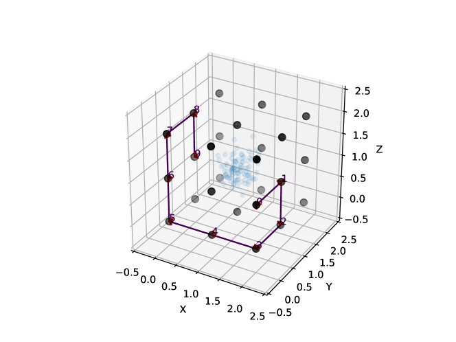
Figure 2: A sample camera trajectory in the Grid dataset.

Results. We choose $\sigma\in\{0.001,0.01,0.1,1,2,3\}$ and at each noise level we run $20$ Monte Carlo random tests. Fig. 3 shows the rotation errors and translation errors of SIM-Sync compared with SE-Sync and SE-Sync+g2o. In both the circle dataset and the grid dataset, SIM-Sync surpasses SE-Sync and SE-Sync+g2o by a (very) small margin, while in the line dataset, SIM-Sync and SE-Sync perform almost the same. Fig. 3 bottom row plots the relative suboptimality $\eta$ (cf. (27)) of SIM-Sync and SE-Sync. We consider the relaxation is not tight if $\eta$ exceeds $0.05$ (the red horizontal dashed line). In the circle dataset and the line dataset, when $\sigma=4$, SE-Sync’s relaxation becomes completely inexact, while SIM-Sync can still achieve tightness, although not always.

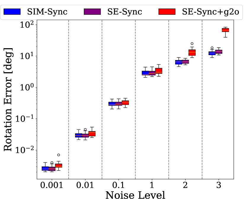
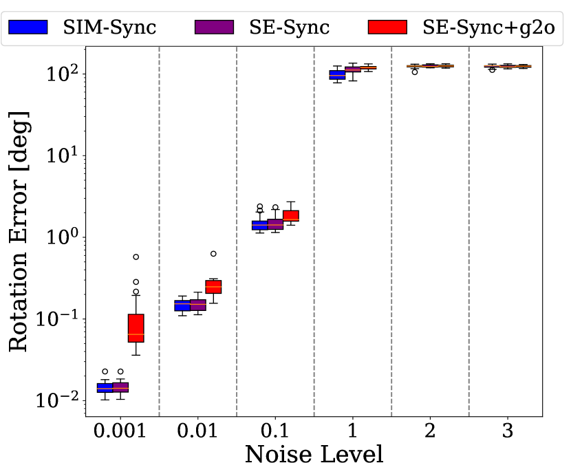
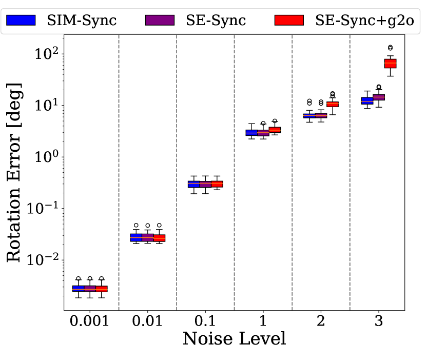
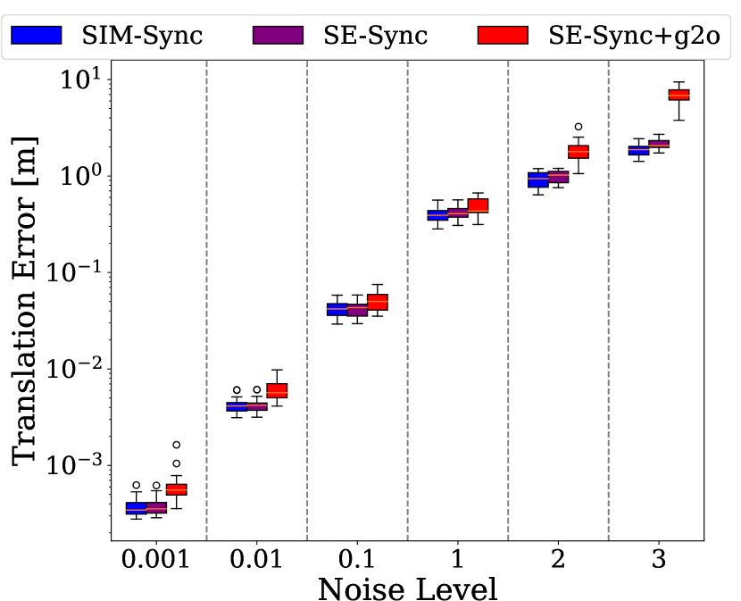
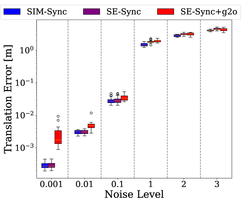
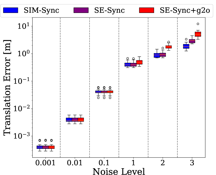
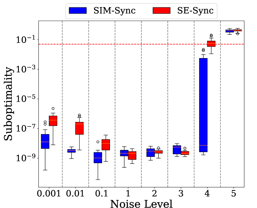
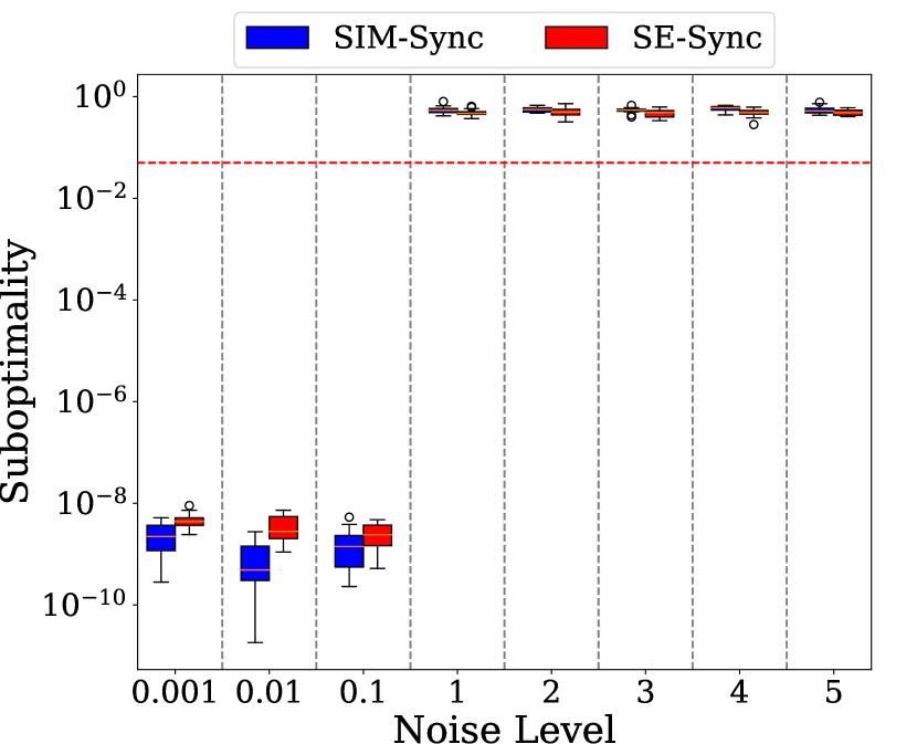
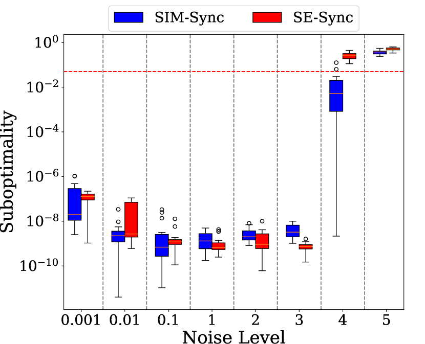
(a) Circle	(b) Grid	(c) Line

Figure 3: Rotation errors (top row), translation errors (middle row), and suboptimality (bottom row) of SIM-Sync, SE-Sync and SE-Sync+g2o in scale-free synchronization.

4.2 Scale Regularization

Setup. We study the effect of the number of poses $N$ and the regularization factor $\lambda$ on the performance of SIM-Sync. We use the same circle, grid, and line datasets in Section 4.1, where the scaling factor is unknown and randomly generated in $[0.9,1.1]$. The noise level $\sigma$ is fixed to $0.01$. For each dataset, we generate $n=100$ points, and vary the number of poses $N\in\{10,50,100,200,400\}$. The regularization factor $\lambda$ is tested with $\{0,1,10,100\}$ for the circle and line datasets, while an additional $\lambda=200$ for the grid dataset. To ensure statistical significance, we perform 20 Monte Carlo simulations for each combination of $N$ and $\lambda$.

Results. Fig. 4(a)(c) plot the averaged scale estimation, rotation error, and translation error w.r.t. number of poses $N$ on the circle dataset and the line dataset, with different colors representing different regularization factors $\lambda$. We observe that (i) as $N$ increases, translation estimation gets slightly worse, but rotation estimation remains unaffected; (ii) the scale estimation does not contract a lot as $N$ increases, even without scale regularization (i.e., $\lambda=0$). Fig. 4(b) shows the same results on the grid dataset, where we clearly observe contraction. Without regularization, the average scale decreases to $0.5$ when $N=400$, which also leads to poor translation estimation. With regularization $\lambda=200$, however, we see that contraction is effectively prevented and the translation error also gets improved. This suggests that regularization improves the performance of SIM-Sync when $N$ is large. It is interesting to see that rotation estimation is not affected by $N$ and $\lambda$. This makes sense because scale and translation are coupled, while rotation is independent. We suspect that the circle graph and the line graph have a certain type of “rigidity” that makes them more robust to contraction, while the grid graph has weaker “rigidity” (i.e., it is easier to bend and twist the trajectory in Fig. 2).

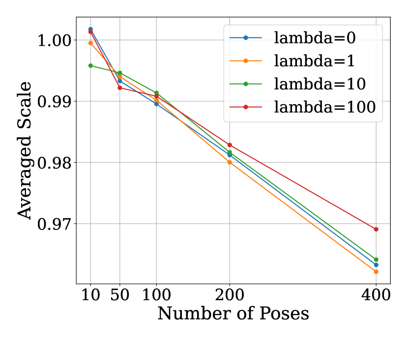
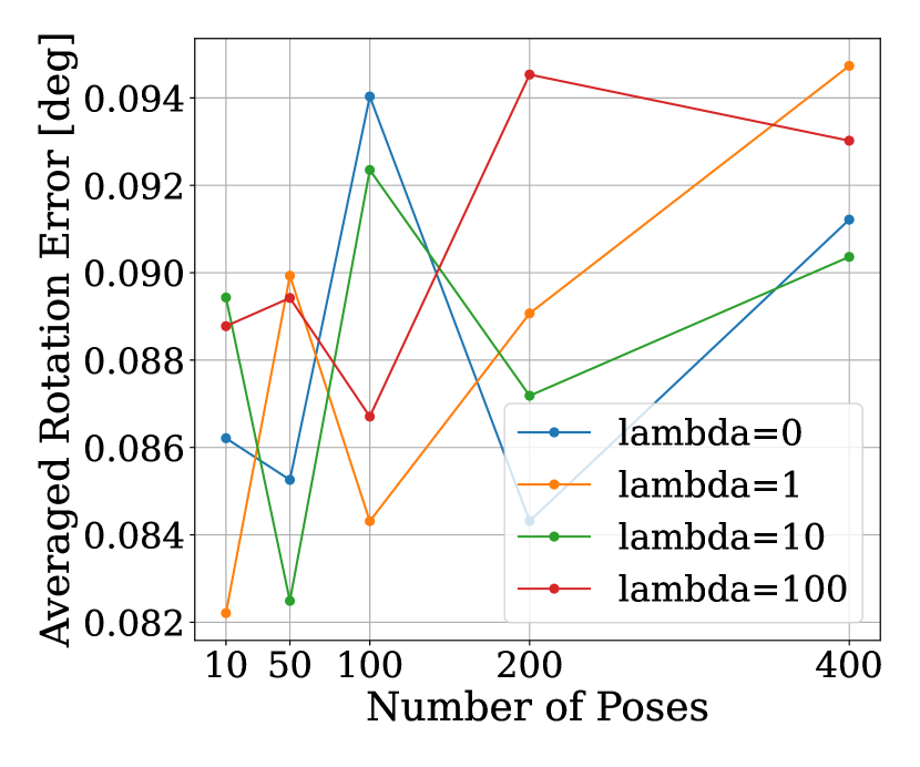
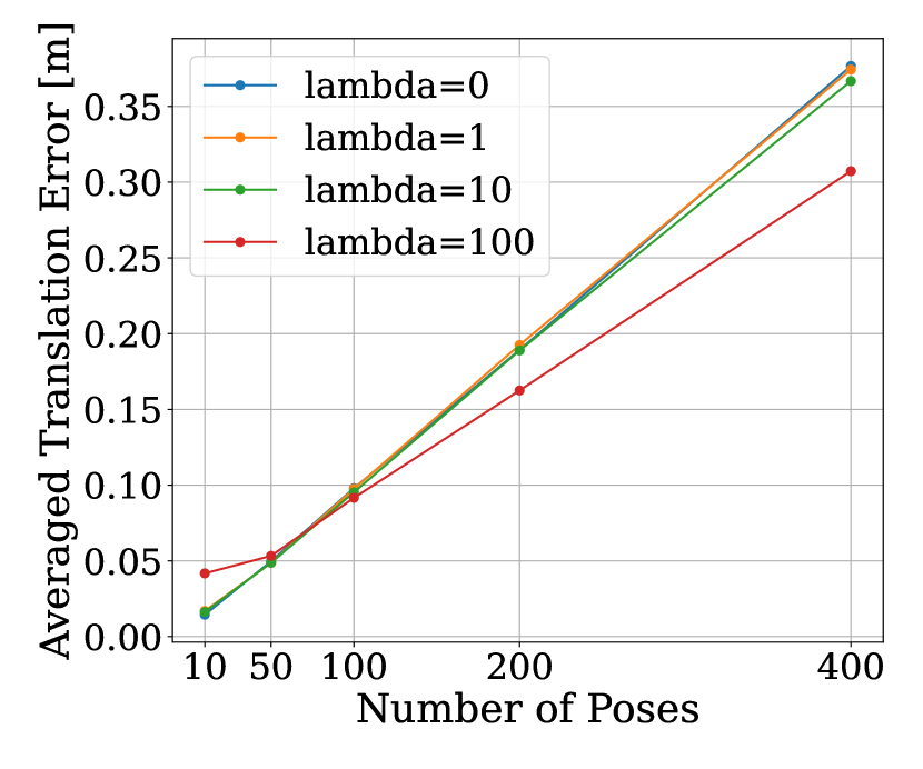
(a) Circle
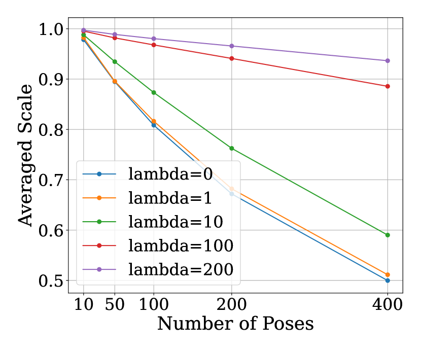
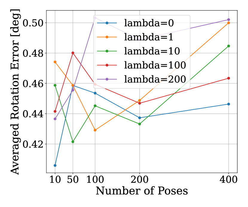
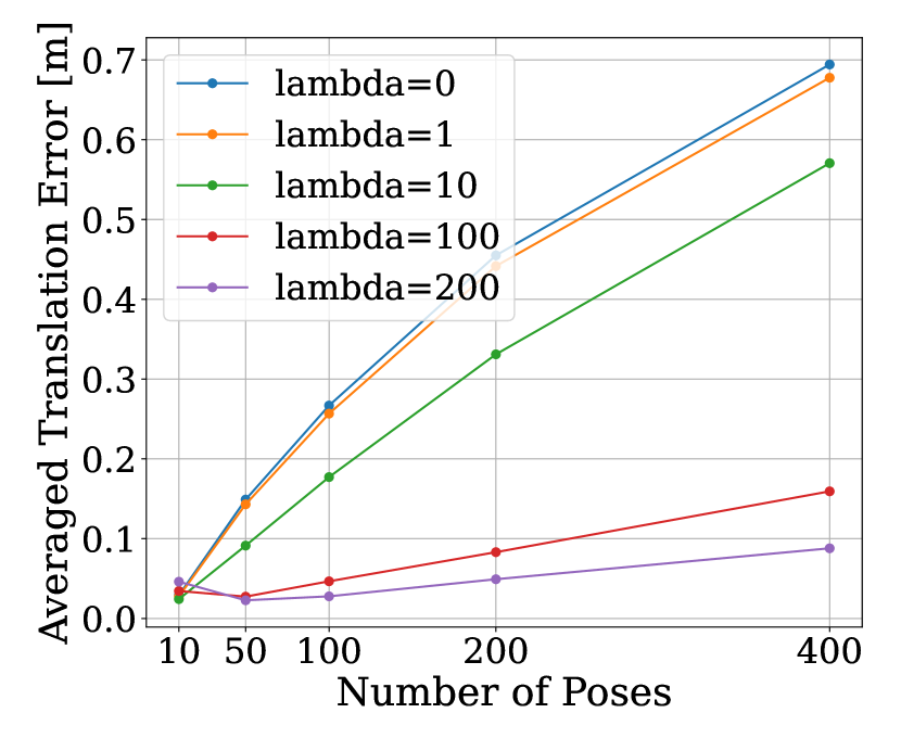
(b) Grid
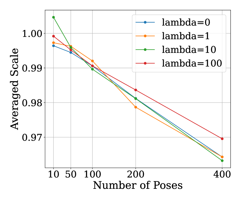
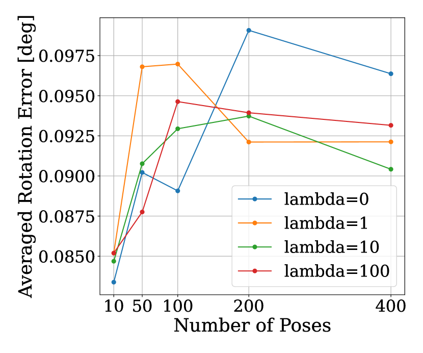
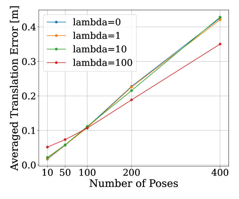
(c) Line

Figure 4: Scale regularization of SIM-Sync in (a) circle, (b) grid, and (c) line datasets.

4.3 Outlier Rejection with Robust Estimators

Setup. We follow the same setup as in previous sections to generate the circle, grid, and line datasets with $N=50$ poses. We sample the scale $s_{i}$ uniformly from $[0.9,1.1]$ and choose the noise $\sigma=0.01$. To generate outliers, we randomly replace a fraction of the edge-wise point correspondences $(\widehat{P}_{i},\widehat{P}_{j})$ with outliers generated from ${\cal N}({\mathbf{0}},{\mathbf{I}}_{3})$. We sweep the outlier rate from $0$ to $90\%$ and perform 20 Monte Carlo simulations at each outlier rate.

Robustify SIM-Sync. We propose three ways to robustify SIM-Sync.

1. SIM-Sync-GNC. This approach directly wraps the SIM-Sync solver in the GNC framework [33] with a truncated least squares (TLS) robust cost function, as shown in the following optimization.

   $$\min_{\begin{subarray}{c}s_{i}>0,R_{i}\in\mathrm{SO}(3),t_{i}\in{{\mathbb{R}}^{3}}\\ i=1,\dots,N\end{subarray}}\sum_{(i,j)\in{\cal E}}\sum_{k=1}^{n_{ij}}\min\left\{\frac{\left\lVert\left(R_{i}{(s_{i}d_{i,k}\widetilde{p}_{i,k})}+t_{i}\right)-\left(R_{j}(s_{j}d_{j,k}\widetilde{p}_{j,k})+t_{j}\right)\right\rVert^{2}}{\beta^{2}},1\right\},$$ (41)

   where $\beta$ is set according to Appendix E.2. To solve (41), SIM-Sync-GNC starts with all weights $w_{ij,k}=1$ in (SIM-Sync) and gradually sets some of the weights to zero based on the residuals.

2. GNC+SIM-Sync. This approach is a two-step algorithm. In step one, we solve the following TLS scaled point cloud registration problem over each edge $(i,j)\in{\cal E}$

   $$\min_{s_{ij}>0,R_{ij}\in\mathrm{SO}(3),t_{ij}\in{{\mathbb{R}}^{3}}}\sum_{k=1}^{n_{ij}}\min\left\{\frac{\|s_{ij}R_{ij}p_{j,k}+t_{ij}-p_{i,k}\|^{2}}{\beta^{2}},1\right\}$$ (42)

   using GNC with a nonminimal solver that we develop, presented in Appendix D, based on Umeyama’s method [30]. $\beta$ is set according to Appendix E.3.

   In step two, we remove all outliers deemed by GNC and solve (SIM-Sync).

3. TEASER+SIM-Sync. Since problem (42) is exactly the problem solved by TEASER [34], we directly apply TEASER to solve (42) and then pass the inliers to (SIM-Sync).

Results. Fig. 5 shows the rotation, translation, and scale estimation errors w.r.t. outlier rates in the circle, grid, and line datasets. We first observe that (i) SIM-Sync-GNC fails at outlier rate $10\%$. This shows that GNC plus a nonminimal solver does not always work, especially when the model to be estimated is high-dimensional and the robust estimation problem is more combinatorial. We then observe that (ii) GNC+SIM-Sync is robust against $50\%$ outliers. This shows that it is a better strategy to first apply GNC to low-dimensional robust fitting. Lastly, we observe that (iii) TEASER+SIM-Sync successfully handles outlier rates of $70\%$ and $80\%$.

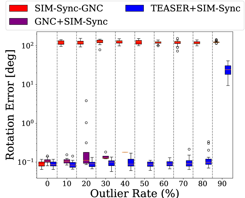
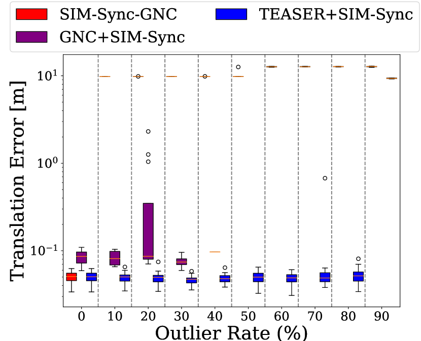
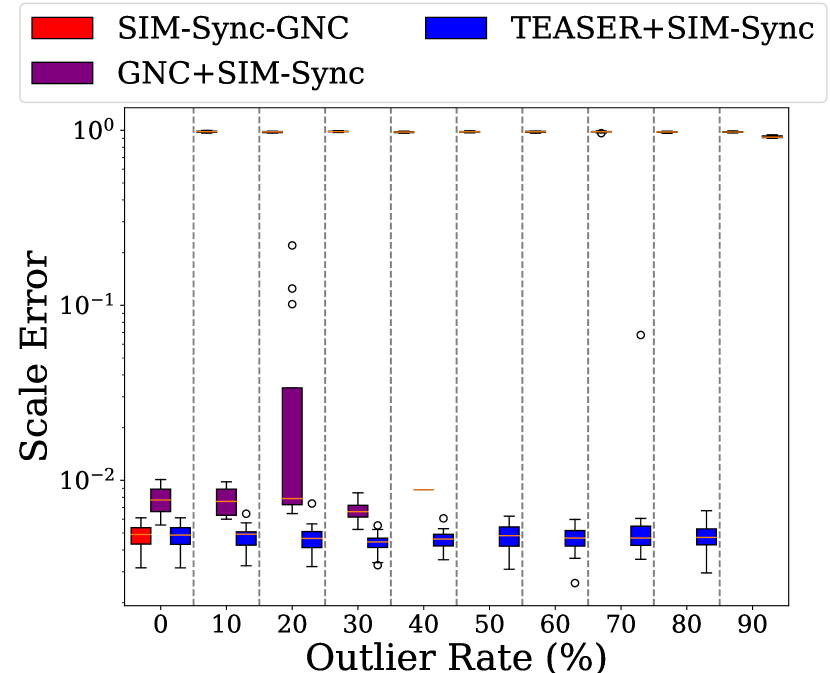
(a) Circle
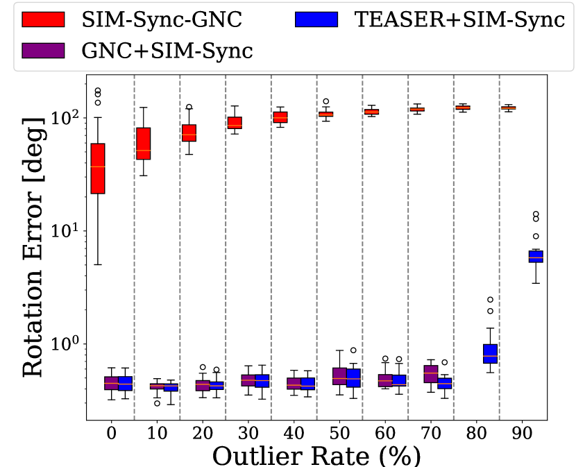
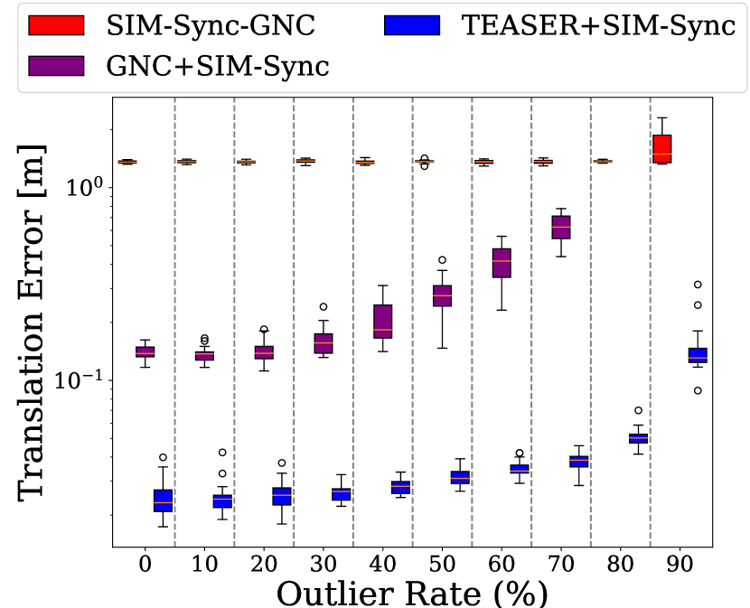
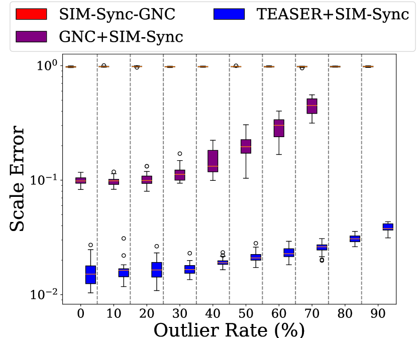
(b) Grid
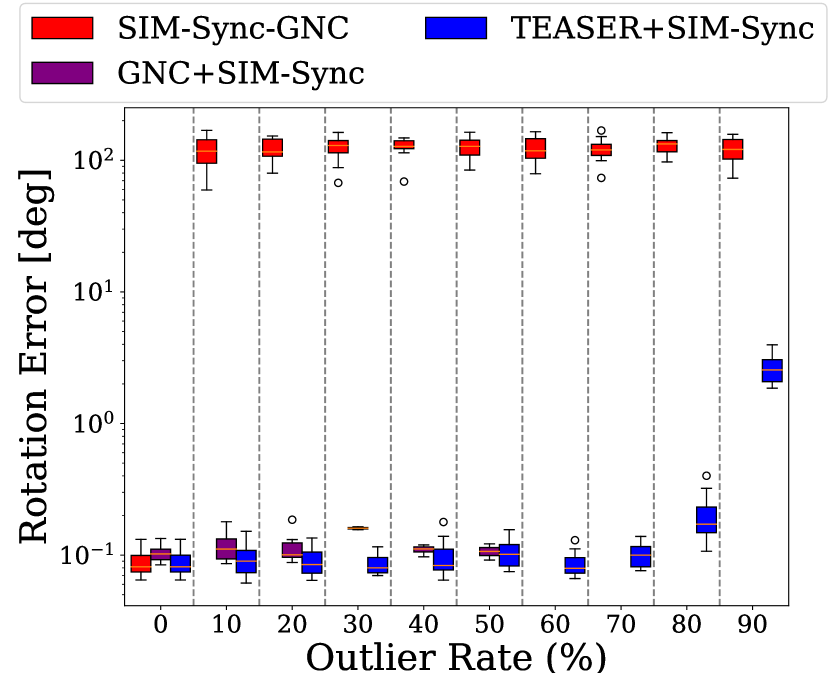
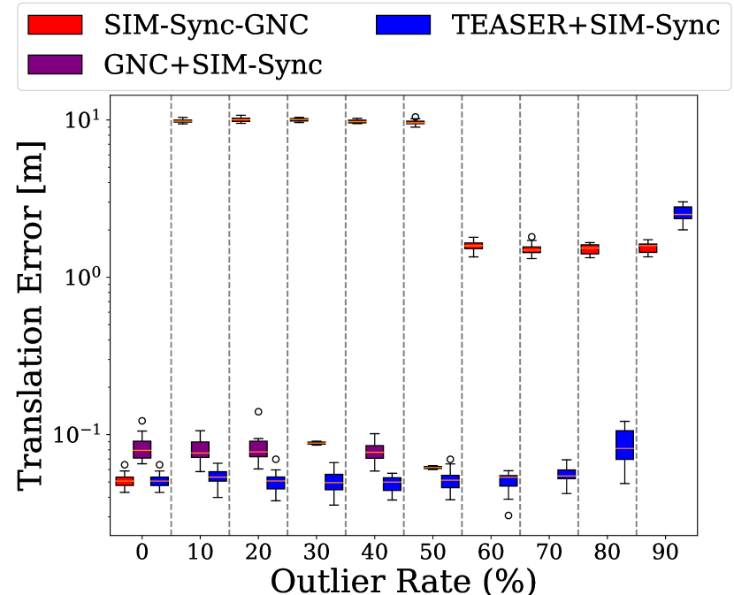
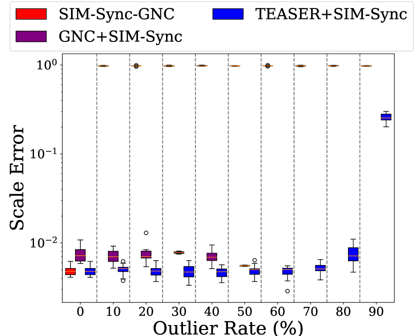
(c) Line

Figure 5: Robustness of SIM-Sync-GNC, GNC+SIM-Sync and TEASER+SIM-Sync in the (a) circle, (b) grid, and (c) line datasets.

4.4 BAL Experiments

Setup. We test two sequences in the bundle adjustment dataset BAL [1]: the dubrovnik-16-22106 sequence and the ladyburg-318-41628 sequence. The former sequence consists of 16 poses with 22,106 points, and the latter sequence consists of 318 poses with 41,628 points. Both sequences provide pixel-wise correspondences for frame pairs, and these correspondences are contaminated with outliers. Since no images are provided, we cannot use a learned module to predict depth. Therefore, we use the $z$-component of the ground truth point position in camera frame $i$, which is computed by using the groundtruth camera pose to transform the point from the global frame to the $i$-th camera frame. Consequently, the scaling effect is not applicable, and we disable the scale prediction. To remove outliers, we use TEASER. We also test the performance of TEASER+SIM-Sync+GT, which uses ground truth poses to filter out outlier correspondences.

Baseline. We compare with two baselines TEASER+SE-Sync and Ceres. TEASER+SE-Sync first uses TEASER to estimate pair-wise relative poses and then feed them into SE-Sync, while Ceres directly optimizes reprojection errors of 3D keypoints. We initialize Ceres as follows: (i) camera intrinsics initialized as groundtruth; (ii) 3D keypoints initialized as groundtruth; (iii) the $z$-component of the camera poses are initialized using groundtruth; (iv) the other components of the camera poses are initialized to be zeros. We remark that this initialization strategy using groundtruth values is optimistic. We also combine TEASER+SIM-Sync and TEASER+SE-Sync with Ceres, i.e., we use the estimation from TEASER+SIM-Sync and TEASER+SE-Sync to initialize Ceres.

Results. Table 1 shows the quantitative results for the dubrovnik-16-22106 sequence (the rotation error and the translation error are averaged over all the nodes). We can see that (i) in the ideal case where outliers are filtered, TEASER+SIM-Sync+GT achieves very accurate reconstruction; (ii) TEASER+SIM-Sync and TEASER+SE-Sync perform worse than TEASER+SIM-Sync+GT, but with the refinement of Ceres, the final results are accurate as well. In fact, they are better than using Ceres alone. Fig. 6 shows qualitative results of the reconstruction, where ICP is used to refine the reconstruction. Both TEASER+SIM-Sync and TEASER+SE-Sync did not use Ceres refinement. We see that TEASER+SIM-Sync already achieves good reconstruction without ICP and Ceres.

Table 2 shows the results for the ladyburg-318-41628 sequence. We observe that TEASER+SIM-Sync+GT still performs quite well. However, both TEASER+SIM-Sync and TEASER+SE-Sync fail to produce accurate pose estimation, though their results are better than Ceres. In fact we see that both TEASER+SIM-Sync and TEASER+SE-Sync lose tightness (suboptimality is around $10\%$ and $20\%$). This suggests that the correspondences provided in this sequence is contaminated by a higher amount of outliers (compared with the dubrovnik-16-22106 sequence) and the point clouds are also noisier. Fig. 7 shows the qualitative reconstruction results.

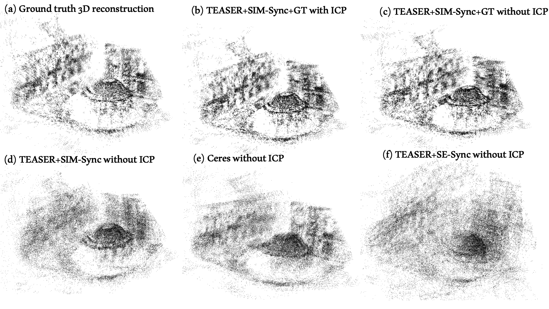
Figure 6: 3D reconstruction of a front view street scene from BAL dubrovnik_16 sequence.

Table 1: Rotation error, translation error and suboptimality of TEASER+SIM-Sync+GT, TEASER+SIM-Sync, TEASER+SE-Sync and Ceres in BAL dataset dubrovnik_16 sequence.

	TEASER+SIM-Sync+GT	TEASER+SIM-Sync		TEASER+SE-Sync		Ceres
		w/o Ceres	w Ceres	w/o Ceres	w Ceres
Rotation Error [deg]	$0.615$	$8.041$	$2.031$	$16.287$	$2.009$	$2.837$
Translation Error [m]	$0.271$	$3.564$	$1.634$	$4.393$	$1.828$	$2.586$
Suboptimality	$1.578\mathrm{e-}9$	$2.996\mathrm{e-}9$	/	$9.651\mathrm{e-}10$	/	/

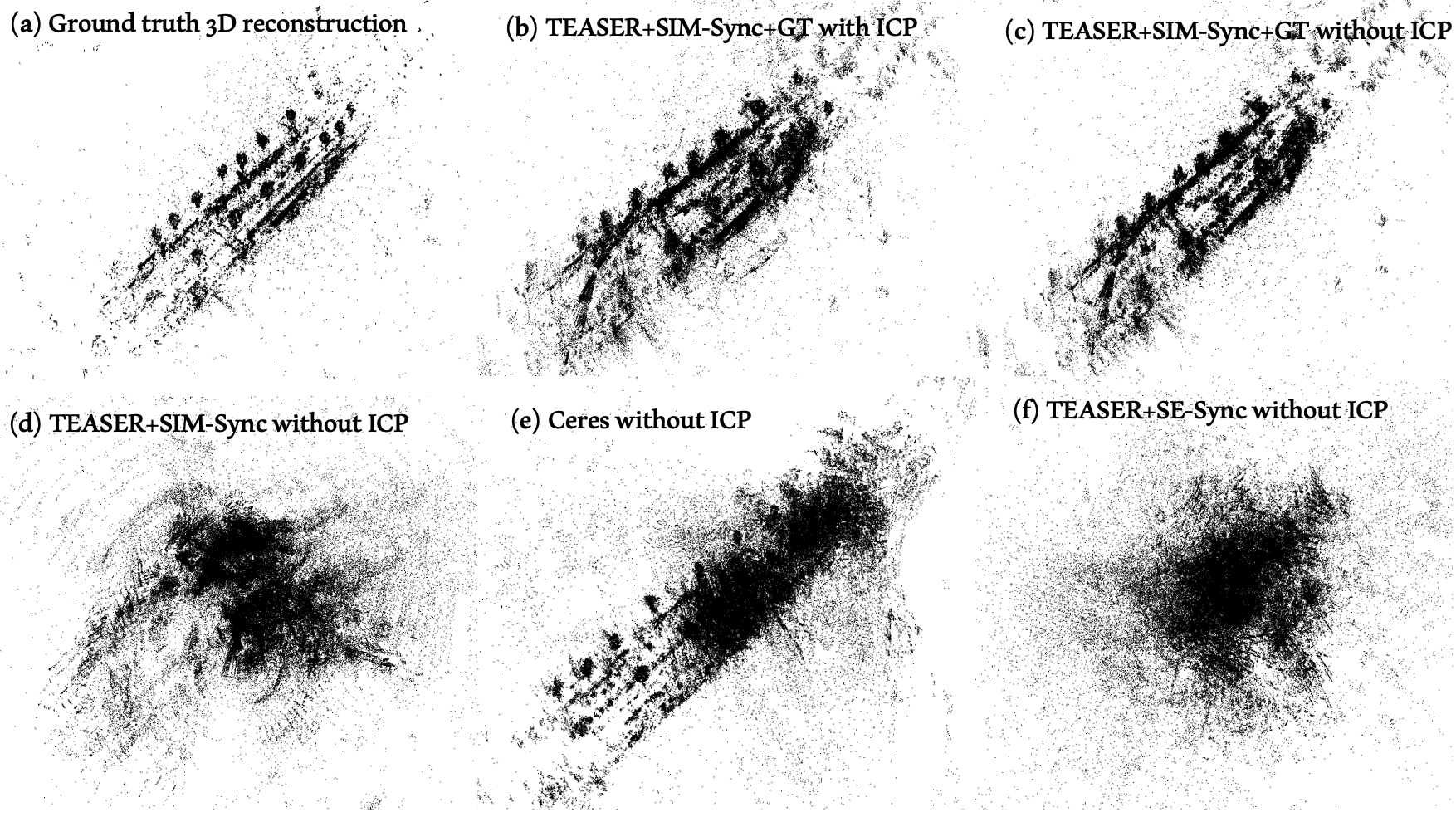
Figure 7: 3D reconstruction of a bird view street scene from BAL ladyburg_318 dataset.

Table 2: Rotation error, translation error and suboptimality of TEASER+SIM-Sync+GT, TEASER+SIM-Sync, TEASER+SE-Sync and Ceres in BAL dataset ladyburg_318 sequence.

	TEASER+SIM-Sync+GT	TEASER+SIM-Sync		TEASER+SE-Sync		Ceres
		w/o Ceres	w Ceres	w/o Ceres	w Ceres
Rotation Error [deg]	$9.730$	$78.457$	$75.046$	$86.067$	$87.995$	$82.601$
Translation Error [m]	$0.334$	$2.299$	$3.307$	$2.600$	$5.858$	$4.776$
Suboptimality	$0.021$	$0.092$	/	$0.216$	/	/

4.5 TUM Experiments

Setup. We test two sequences in the TUM dataset, the first 200 frames in the freiburg1_xyz sequence and the first 200 frames in the freiburg2_xyz sequence, respectively. For TEASER+SIM-Sync, we use learned depth obtained from the MiDaS-v3 model [23, 6], with the largest 10% depth discarded. Note that MiDaS-v3 is not trained on the TUM dataset, and we directly use its default parameter configuration (i.e., zero-shot). For TEASER+SIM-Sync+GTDepth, we use ground truth depth. We conduct two tests for TEASER+SIM-Sync/TEASER+SIM-Sync+GTDepth. In the first test, we run TEASER+SIM-Sync/TEASER+SIM-Sync+GTDepth on the essential graph (EG), which is a set of key frames and edges selected by the ORB-SLAM3 [8] algorithm. In the second test, we run TEASER+SIM-Sync/TEASER+SIM-Sync+GTDepth on a graph ${\cal G}=({\cal V},{\cal E})$ generated as follows

$${\cal E}=\left\{(i,j)\mid i=1,2,\ldots,N-2,\text{ and }j=i+1\text{ or }j=i+2\text{ or }(i=N-1\text{ and }j=N)\right\},$$ (43)

i.e., we sample the frame pairs of neighboring 3 frames. We utilize SIFT [19] to get initial correspondences and then apply the learned CAPS descriptor [31] to sort the correspondences by the feature similarity between two points. We keep a maximum of 400 SIFT correspondences.

Baseline. We use the state-of-the-art visual SLAM algorithm ORB-SLAM3 [8] as a baseline. We use Monocular mode without IMU of ORB-SLAM3 and run on its default setting in the official script of running TUM dataset. We also compare with the stereo mode of ORB-SLAM3.

Results. We take a detour first to demonstrate how TEASER works as shown in Fig. 8. We randomly pick a pair of images from TEASER+SIM-Sync+GTDepth and TEASER+SIM-Sync. The red lines indicate outlier correspondences detected by TEASER while the green lines are inliers. We can see that TEASER performs quite well in classifying outliers from inliers.

Tables 3 and 4 show the quantitative results of all methods in the freiburg1_xyz and freiburg2_xyz sequences, respectively. We follow the standard evaluation protocol of visual odometry for assessing pose accuracy, i.e., Absolute Trajectory Error (ATE) and Relative Pose Error (RPE). Since the scale of the output of ORB-SLAM3 is unknown, we scale up the predicted translation to the scale of the groundtruth. We can see that TEASER+SIM-Sync+GTDepth and TEASER+SIM-Sync with Essential Graph achieve comparable accuracy as ORB-SLAM3, while being simpler and more direct algorithms that also offer optimality guarantees. On the other hand, TEASER+SIM-Sync+GTDepth and TEASER+SIM-Sync with the naive graph as in (43) show worse accuracy. This result implies that the essential graph is a better graph architecture than the naive graph in scene reconstruction.

We show the qualitative 3D reconstruction results of the freiburg1_xyz and freiburg2_xyz sequences in Fig. 9, using TEASER+SIM-Sync with learned depth. The reconstruction is formed by stacking the learned depth point clouds of all frames (after transformation to a common coordinate frame).

We can see that even with learned depth, the TEASER+SIM-Sync reconstruction achieves good accuracy.

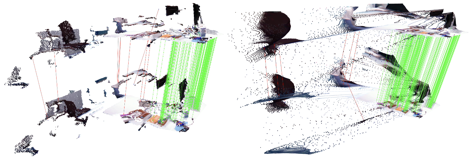
Figure 8: Illustration of outlier detection by TEASER. (Left: TEASER+SIM-Sync+GTDepth, Right: TEASER+SIM-Sync with learned depth)

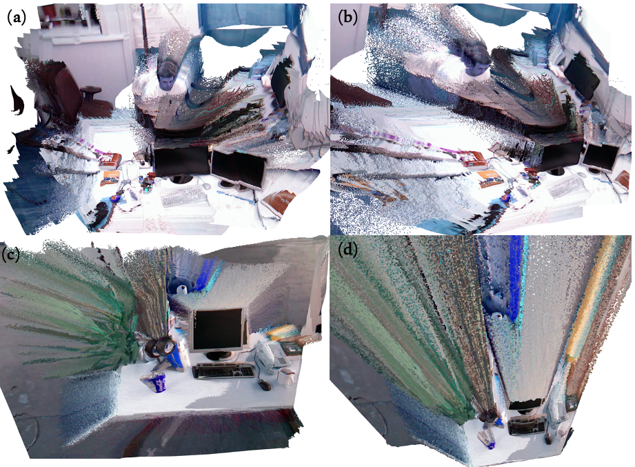
Figure 9: 3D reconstruction of TEASER+SIM-Sync with learned depth in TUM. (a) Forward view reconstruction and (b) Side view reconstruction in the freiburg1_xyz sequence. (c) Forward view reconstruction and (d) Bird view reconstruction in the freiburg2_xyz sequence.

Table 3: Rotation and translation error comparison for TEASER+SIM-Sync+GTDepth, TEASER+SIM-Sync and ORB-SLAM3 in the 200-pose freiburg1_xyz sequence of TUM. We set the regularization factor to $\lambda=3$ for TEASER+SIM-Sync+GTDepth and TEASER+SIM-Sync without essential graph, and $\lambda=0$ with essential graph (EG).

	TEASER+SIM-Sync+GTDepth		TEASER+SIM-Sync		ORB-SLAM3	ORB-SLAM3 (RGB-D)
	w/o EG	w EG	w/o EG	w EG
ATE [m]	$0.2453$	$0.1335$	$0.2003$	$0.0638$	$0.1081$	$0.0147$
RPE Trans [m]	$0.0167$	$0.0097$	$0.0163$	$0.0064$	$0.0068$	$0.0043$
RPE Rot [deg]	$1.2001$	$0.6476$	$1.3320$	$0.5659$	$0.5521$	$0.2813$
Suboptimality	$1.1966\mathrm{e-}9$	$1.1966\mathrm{e-}9$	$3.4336\mathrm{e-}9$	$9.8312\mathrm{e-}11$	/	/

Table 4: Rotation and translation error comparison for TEASER+SIM-Sync+GTDepth, TEASER+SIM-Sync and ORB-SLAM3 in the 200-pose freiburg2_xyz sequence of TUM. Regularization factor same as Table 3.

	TEASER+SIM-Sync+GTDepth		TEASER+SIM-Sync		ORB-SLAM3	ORB-SLAM3 (RGB-D)
	w/o EG	w EG	w/o EG	w EG
ATE [m]	$0.2089$	$0.1237$	$0.3190$	$0.0358$	$0.0246$	$0.1023$
RPE Trans [m]	$0.0072$	$0.0017$	$0.0030$	$0.0012$	$0.0007$	$0.0017$
RPE Rot [deg]	$0.3586$	$0.2349$	$0.9982$	$0.2240$	$0.2155$	$0.1739$
Suboptimality	$9.8904\mathrm{e-}10$	$1.7527\mathrm{e-}9$	$2.7516\mathrm{e-}9$	$6.1298\mathrm{e-}10$	/	/

5 Conclusions

We introduced SIM-Sync, a certifiably optimal algorithm for camera trajectory estimation and scene reconstruction directly from image-level correspondences. With a pretrained depth prediction network, 2D image keypoints are lifted to 3D scaled point clouds, and SIM-Sync seeks to jointly synchronize camera poses and unknown (per-image) scaling factors to minimize the sum of Euclidean distances between matching points. By first developing a QCQP formulation and then applying semidefinite relaxation, SIM-Sync can achieve certifiable global optimality. We demonstrate the tightness, (outlier-)robustness, and practical usefulness of SIM-Sync in both simulated and real datasets. Future research aims to (i) speed up SIM-Sync by exploiting low-rankness of the optimal SDP solutions [24, 35], and (ii) leverage the 3D reconstruction from SIM-Sync to improve the imperfect depth prediction from the pretrained model.

Appendix

Appendix A Proof of Proposition 1

Proof.

Let

$$P_{i}= \left[\begin{array}[]{ccc}\sqrt{w_{ij,1}}d_{i,1}\widetilde{p}_{i,1}&\cdots&\sqrt{w_{ij,n_{ij}}}d_{i,n_{ij}}\widetilde{p}_{i,n_{ij}}\end{array}\right]\in{{\mathbb{R}}^{3\times n_{ij}}},\quad i=1,\dots,N,$$ (A45)

$$W_{ij}= [\sqrt{w_{ij,1}},\dots,\sqrt{w_{ij,n_{ij}}}]^{\mathsf{T}}\in{{\mathbb{R}}^{n_{ij}}},\quad(i,j)\in{\cal E},$$

For any $t_{i}$ and $\mathrm{vec}\left(s_{i}R_{i}\right)$, define the selection matrices

$$t_{i}=Z^{t}_{i}t,\quad\mathrm{vec}\left(s_{i}R_{i}\right)=Z^{R}_{i}r,\quad Z^{t}_{i}\in{{\mathbb{R}}^{3\times 3N}},\quad Z^{R}_{i}\in{{\mathbb{R}}^{9\times 9N}}.$$

We then write the objective in (SIM-Sync) as

$$L(t,r)= \displaystyle\sum_{(i,j)\in{\cal E}}\left\lVert(s_{i}R_{i})P_{i}+t_{i}W_{ij}^{\mathsf{T}}-(s_{j}R_{j})P_{j}-t_{j}W_{ij}^{\mathsf{T}}\right\rVert_{F}^{2}$$

$$= \displaystyle\sum_{(i,j)\in{\cal E}}\left\lVert(P_{i}^{\mathsf{T}}\otimes{\mathbf{I}}_{3})\mathrm{vec}\left(s_{i}R_{i}\right)+(W_{ij}\otimes{\mathbf{I}}_{3})t_{i}-(P_{j}^{\mathsf{T}}\otimes{\mathbf{I}}_{3})\mathrm{vec}\left(s_{j}R_{j}\right)-(W_{ij}\otimes{\mathbf{I}}_{3})t_{j}\right\rVert^{2}$$

$$= \displaystyle\sum_{(i,j)\in{\cal E}}\left\lVert\underbrace{\left[(P_{i}^{\mathsf{T}}\otimes{\mathbf{I}}_{3})Z^{R}_{i}-(P_{j}^{\mathsf{T}}\otimes{\mathbf{I}}_{3})Z^{R}_{j}\right]}_{=:C_{ij}^{R}}r+\underbrace{\left[(W_{ij}\otimes{\mathbf{I}}_{3})Z^{t}_{i}-(W_{ij}\otimes{\mathbf{I}}_{3})Z^{t}_{j}\right]}_{=:C_{ij}^{t}}t\right\rVert^{2}$$ (A46)

Note that $Z^{R}_{i}$ and $Z^{t}_{i}$ can actually be decomposed as

$$Z^{R}_{i}= e_{i}^{\mathsf{T}}\otimes{\mathbf{I}}_{3}\otimes{\mathbf{I}}_{3}$$

$$Z^{t}_{i}= e_{i}^{\mathsf{T}}\otimes{\mathbf{I}}_{3}$$

where $e_{i}\in{{\mathbb{R}}^{N}}$ is the basis vector in ${{\mathbb{R}}^{N}}$ where the $i^{th}$ entry is 1 while other entries are all 0’s. Plug in $C_{ij}^{R}$ and $C_{ij}^{t}$, we obtain:

$$C_{ij}^{R}= (P_{i}^{\mathsf{T}}\otimes{\mathbf{I}}_{3})(e_{i}^{\mathsf{T}}\otimes{\mathbf{I}}_{3}\otimes{\mathbf{I}}_{3})-(P_{j}^{\mathsf{T}}\otimes{\mathbf{I}}_{3})(e_{j}^{\mathsf{T}}\otimes{\mathbf{I}}_{3}\otimes{\mathbf{I}}_{3})$$

$$= (P_{i}^{\mathsf{T}}(e_{i}^{\mathsf{T}}\otimes{\mathbf{I}}_{3}))\otimes{\mathbf{I}}_{3}-(P_{j}^{\mathsf{T}}(e_{j}^{\mathsf{T}}\otimes{\mathbf{I}}_{3}))\otimes{\mathbf{I}}_{3}$$

$$= ((1\otimes P_{i}^{\mathsf{T}})(e_{i}^{\mathsf{T}}\otimes{\mathbf{I}}_{3}))\otimes{\mathbf{I}}_{3}-((1\otimes P_{j}^{\mathsf{T}})(e_{j}^{\mathsf{T}}\otimes{\mathbf{I}}_{3}))\otimes{\mathbf{I}}_{3}$$

$$= (e_{i}^{\mathsf{T}}\otimes P_{i}^{\mathsf{T}})\otimes{\mathbf{I}}_{3}-(e_{j}^{\mathsf{T}}\otimes P_{j}^{\mathsf{T}})\otimes{\mathbf{I}}_{3}$$

$$= (e_{i}^{\mathsf{T}}\otimes P_{i}^{\mathsf{T}}-e_{j}^{\mathsf{T}}\otimes P_{j}^{\mathsf{T}})\otimes{\mathbf{I}}_{3}$$

$$C_{ij}^{t}= (W_{ij}\otimes{\mathbf{I}}_{3})(e_{i}^{\mathsf{T}}\otimes{\mathbf{I}}_{3})-(W_{ij}\otimes{\mathbf{I}}_{3})(e_{j}^{\mathsf{T}}\otimes{\mathbf{I}}_{3})$$

$$= (W_{ij}e_{i}^{\mathsf{T}})\otimes{\mathbf{I}}_{3}-(W_{ij}e_{j}^{\mathsf{T}})\otimes{\mathbf{I}}_{3}$$

$$= (W_{ij}e_{i}^{\mathsf{T}}-W_{ij}e_{j}^{\mathsf{T}})\otimes{\mathbf{I}}_{3}$$

Plug $C_{ij}^{R}$ and $C_{ij}^{t}$ back to (A46), we then simplify the objective as:

$$L(t,r)= \displaystyle\sum_{(i,j)\in{\cal E}}\left\lVert((e_{i}^{\mathsf{T}}\otimes P_{i}^{\mathsf{T}}-e_{j}^{\mathsf{T}}\otimes P_{j}^{\mathsf{T}})\otimes{\mathbf{I}}_{3})r+((W_{ij}e_{i}^{\mathsf{T}}-W_{ij}e_{j}^{\mathsf{T}})\otimes{\mathbf{I}}_{3})t\right\rVert^{2}$$

$$= \displaystyle\left[\begin{array}[]{c}t\\ r\end{array}\right]^{\mathsf{T}}\left(\left[\begin{array}[]{cc}Q_{1}&V^{\mathsf{T}}\\ V&Q_{2}\end{array}\right]\otimes{\mathbf{I}}_{3}\right)\left[\begin{array}[]{c}t\\ r\end{array}\right]$$ (A53)

$$= \displaystyle t^{\mathsf{T}}\left(Q_{1}\otimes{\mathbf{I}}_{3}\right)t+2r^{\mathsf{T}}\left(V\otimes{\mathbf{I}}_{3}\right)t+r^{\mathsf{T}}\left(Q_{2}\otimes{\mathbf{I}}_{3}\right)r$$ (A54)

where

$$Q_{1}= \displaystyle\sum_{(i,j)\in{\cal E}}(W_{ij}e_{i}^{\mathsf{T}}-W_{ij}e_{j}^{\mathsf{T}})^{\mathsf{T}}(W_{ij}e_{i}^{\mathsf{T}}-W_{ij}e_{j}^{\mathsf{T}})\in{{\mathbb{R}}^{N\times N}}$$ (A55)

$$Q_{2}= \displaystyle\sum_{(i,j)\in{\cal E}}(e_{i}^{\mathsf{T}}\otimes P_{i}^{\mathsf{T}}-e_{j}^{\mathsf{T}}\otimes P_{j}^{\mathsf{T}})^{\mathsf{T}}(e_{i}^{\mathsf{T}}\otimes P_{i}^{\mathsf{T}}-e_{j}^{\mathsf{T}}\otimes P_{j}^{\mathsf{T}})\in{{\mathbb{R}}^{3N\times 3N}}$$

$$V= \displaystyle\sum_{(i,j)\in{\cal E}}(e_{i}^{\mathsf{T}}\otimes P_{i}^{\mathsf{T}}-e_{j}^{\mathsf{T}}\otimes P_{j}^{\mathsf{T}})^{\mathsf{T}}(W_{ij}e_{i}^{\mathsf{T}}-W_{ij}e_{j}^{\mathsf{T}})\in{{\mathbb{R}}^{3N\times N}}$$

concluding the proof. ∎

Appendix B Proof of Proposition 2

Proof.

To represent $t$ as a function of $r$, simply take the gradient of (6) w.r.t. $t$ and setting it to zero, we obtain

$$(Q_{1}\otimes{\mathbf{I}}_{3}){t}=(V\otimes{\mathbf{I}}_{3})^{\mathsf{T}}r.$$ (A56)

Proposition A6 (Laplacian Representation of $Q_{1}$).

$Q_{1}$ can be represented as:

$$Q_{1}=L({\cal G})$$ (A57)

where $L({\cal G})$ is the Laplacian of ${\cal G}$.

Proof.

Note that ${\cal G}$ is a weighted undirected graph. Calling $\delta(i)$ for the set of edges incident to a vertex $v$ and $n_{e}=n_{ij},w_{e,k}=w_{ij,k}$ for $e=(i,j)$, the Laplacian of ${\cal G}$ is:

$$L({\cal G})_{ij}=\begin{cases}\sum_{e\in\delta(i)}\sum_{k=1}^{n_{e}}\sqrt{w_{e,k}}&\text{if }i=j,\\ -\sum_{k=1}^{n_{ij}}\sqrt{w_{ij,k}}&\text{if }(i,j)\in{\cal E},\\ 0&\text{if }(i,j)\notin{\cal E}.\end{cases}$$ (A58)

On the other hand, by expanding (A55) and compare it with (A58), we finish the proof. ∎

Note that $\mathrm{rank}\left(L({\cal G})\right)=N-1$, then $\mathrm{rank}\left(Q_{1}\otimes{\mathbf{I}}_{3}\right)=\mathrm{rank}\left(L({\cal G})\right)\mathrm{rank}\left({\mathbf{I}}_{3}\right)$ by Proposition A6. Thus $Q_{1}\otimes{\mathbf{I}}_{3}$ is not invertible. As we fixed $s_{1}=1$, $R_{1}={\mathbf{I}}_{3}$, $t_{1}=0$, $t$ has a unique solution. Calling $\bar{t}=[t_{2};\dots;t_{N}]\in{{\mathbb{R}}^{3N-3}}$ and $\bar{Q}_{1}=[c_{2};\dots;c_{N}]\in{{\mathbb{R}}^{N\times(N-1)}}$ where $c_{i}$ is the ith column of $Q_{1}$. We have

$$(\bar{Q}_{1}\otimes{\mathbf{I}}_{3}){\bar{t}}=(V\otimes{\mathbf{I}}_{3})^{\mathsf{T}}r$$ (A59)

Since $\mathrm{rank}\left(L({\cal G})\right)=N-1$ and $\sum_{i=1,..,N}c_{i}=\mathbf{0}_{N}$, then $span(c_{1},...,c_{n})=span(c_{2},...,c_{n})$ and $\mathrm{rank}\left(\bar{Q}_{1}\right)=N-1$ which implies that $\bar{Q}_{1}$ has full column rank. Hence, by taking inverse and rearrange, we obtain

$$\bar{t}= \left(\bar{A}\otimes{\mathbf{I}}_{3}\right)r$$ (A60)

where

$$\bar{A}= -(\bar{Q}_{1}^{\mathsf{T}}\bar{Q}_{1})^{-1}\bar{Q}_{1}^{\mathsf{T}}V^{\mathsf{T}}$$ (A61)

Together with $t_{1}=0$,

$$t= \left(A\otimes{\mathbf{I}}_{3}\right)r$$ (A62)

with

$$A= \left[\begin{array}[]{c}{\mathbf{0}}_{1\times 3N}\\ -(\bar{Q}_{1}^{\mathsf{T}}\bar{Q}_{1})^{-1}\bar{Q}_{1}^{\mathsf{T}}V^{\mathsf{T}}\end{array}\right]\in{{\mathbb{R}}^{N\times 3N}}$$ (A65)

Now we have a closed form solution of $t$. Plug in the solution of $t$ into (A54), we obtain:

$$L(r)= \displaystyle r^{\mathsf{T}}\left(\left(A^{\mathsf{T}}Q_{1}A+VA+A^{\mathsf{T}}V^{\mathsf{T}}+Q_{2}\right)\otimes{\mathbf{I}}_{3}\right)r$$ (A66)

Note that

$$r= \mathrm{vec}\left(R\right)$$ (A67)

Then $L(r)$ is equivalent to

$$L(R)= \displaystyle\mathrm{vec}\left(R\right)^{\mathsf{T}}\left(\left(A^{\mathsf{T}}Q_{1}A+VA+A^{\mathsf{T}}V^{\mathsf{T}}+Q_{2}\right)\otimes{\mathbf{I}}_{3}\right)\mathrm{vec}\left(R\right)$$ (A68)

Rewrite (A68) in a more compact matricized form gives:

$$\rho^{\star}=\min_{R} \mathrm{tr}\left(QR^{\mathsf{T}}R\right)$$ (A69)

$$Q\coloneqq A^{\mathsf{T}}Q_{1}A+VA+A^{\mathsf{T}}V^{\mathsf{T}}+Q_{2}\in\mathbb{S}^{3N},$$ (A70)

concluding the proof. ∎

Appendix C Proof of Proposition 3

Proof.

We first prove (21).

“$\Longrightarrow$”: If $\bar{R}\in\mathfrak{s}\mathrm{O}(3)$, then $\bar{R}=sR$ for some $s\geq 0$ and $R\in\mathrm{O}(3)$. Therefore,

$$\left[\begin{array}[]{ccc}c_{1}^{\mathsf{T}}c_{1}&c_{1}^{\mathsf{T}}c_{2}&c_{1}^{\mathsf{T}}c_{3}\\ &c_{2}^{\mathsf{T}}c_{2}&c_{2}^{\mathsf{T}}c_{3}\\ &*&c_{3}^{\mathsf{T}}c_{3}\end{array}\right]=\bar{R}^{\mathsf{T}}\bar{R}=(sR)^{\mathsf{T}}(sR)=s^{2}R^{\mathsf{T}}R=s^{2}{\mathbf{I}}_{3},$$

which shows the quadratic constraints in (21) must hold.

“$\Longleftarrow$”: Suppose the quadratic constraints in (21) hold. (i) If $c_{i}^{\mathsf{T}}c_{i}=0,i=1,2,3$, then $\bar{R}={\mathbf{0}}\in\mathfrak{s}\mathrm{O}(3)$ trivially holds. (ii) If $c_{i}^{\mathsf{T}}c_{i}=\alpha>0,i=1,2,3$, then $\bar{R}$ can be written as

$$\bar{R}=\sqrt{\alpha}\left[\begin{array}[]{ccc}u_{1}&u_{2}&u_{3}\end{array}\right],$$

where $u_{i},i=1,2,3$ are unit vectors. However,

$$c_{i}^{\mathsf{T}}c_{j}=0\Longleftrightarrow\alpha u_{i}^{\mathsf{T}}u_{j}=0\Longleftrightarrow u_{i}^{\mathsf{T}}u_{j}=0,\quad\forall i\neq j,$$

which means $(u_{1},u_{2},u_{3})$ are orthogonal to each other and therefore $[u_{1},u_{2},u_{3}]\in\mathrm{O}(3)$.

We then show that if an optimal solution of (QCQP) satisfies (22), then it must be an optimizer of (13). First note that (QCQP) is a relaxation of (13) and $\rho_{{\sf QCQP}}^{\star}\leq\rho^{\star}$. This is because any feasible solution to (13) must also be feasible to (QCQP), due to the fact that any scaled rotation must also lie in $\mathfrak{s}\mathrm{O}(3)$ by its definition (19). However, if $R^{\star}$ satisfies (22), then we claim that $R^{\star}$ is also feasible to (13) (hence also optimal to (13)), i.e., each $\bar{R}_{i}^{\star}$ can be written as a scaled rotation. In fact, $\bar{R}_{i}^{\star}\in\mathfrak{s}\mathrm{O}(3)$ implies $\bar{R}_{i}^{\star}=s_{i}^{\star}R_{i}^{\star}$ for some $s_{i}^{\star}\geq 0$ and $R_{i}^{\star}\in\mathrm{O}(3)$. However,

$$\det{\bar{R}_{i}^{\star}}=(s_{i}^{\star})^{3}\det R_{i}^{\star}>0$$

implies $s_{i}^{\star}\neq 0$ and $R_{i}^{\star}\in\mathrm{SO}(3)$, because any matrix in $\mathrm{O}(3)$ is either a rotation (with $+1$ determinant) or a reflection (with $-1$ determinant). ∎

Appendix D Weighted Scaled Point Cloud Registration

Consider the optimization problem where $\{(Y_{i},X_{i}),i=1,...,n\}$ are matching scaled point clouds and we seek the best similarity transformation between them

$$\min_{\begin{subarray}{c}s>0,R\in\mathrm{SO}(3),t\in{{\mathbb{R}}^{3}}\\ i=1,\dots,n\end{subarray}}\sum_{i=1}^{n}w_{i}\left\lVert sRX_{i}+t-Y_{i}\right\rVert^{2},$$ (A71)

where $w_{i},i=1,\dots,n$ are known weights. We will show that problem (A71) admits a closed-form solution.

Let the objective function be

$$f=\sum_{i=1}^{n}w_{i}\left\lVert sRX_{i}+t-Y_{i}\right\rVert^{2}.$$ (A72)

Firstly, take the derivative with respect to $t$:

$$\frac{\partial f}{\partial t}=2\sum_{i}w_{i}(sRX_{i}+t-Y_{i})$$ (A73)

Set it to zero, we obtain:

$$t=\mu_{y}-sR\mu_{x}$$ (A74)

where

$$\mu_{y}=\frac{\sum_{i}w_{i}y_{i}}{\sum_{i}w_{i}}$$ (A75)

$$\mu_{x}=\frac{\sum_{i}w_{i}x_{i}}{\sum_{i}w_{i}}$$ (A76)

Substitute $t$ with (A74) in original optimization, we obtain:

$$f= \sum_{i=1}^{n}w_{i}\left\lVert sR\left[X_{i}-\mu_{x}\right]-(Y_{i}-\mu_{y})\right\rVert^{2}$$ (A77)

$$= \sum_{i=1}^{n}\left\lVert\sqrt{w_{i}}sR\left[X_{i}-\mu_{x}\right]-\sqrt{w_{i}}(Y_{i}-\mu_{y})\right\rVert^{2}$$ (A78)

$$= \sum_{i=1}^{n}\left\lVert R\left[\sqrt{w_{i}}s(X_{i}-\mu_{x})\right]-\sqrt{w_{i}}(Y_{i}-\mu_{y})\right\rVert^{2}$$ (A79)

Let

$$A=\left[\begin{array}[]{ccc}\sqrt{w_{1}}(Y_{1}-\mu_{y})&\cdots&\sqrt{w_{n}}(Y_{n}-\mu_{y})\end{array}\right]\in{{\mathbb{R}}^{3\times n}},$$ (A81)

$$B=\left[\begin{array}[]{ccc}\sqrt{w_{1}}(X_{1}-\mu_{x})&\cdots&\sqrt{w_{n}}(X_{n}-\mu_{x})\end{array}\right]\in{{\mathbb{R}}^{3\times n}}$$ (A83)

Then $f$ is simplified as:

$$f=\left\lVert R\cdot(sB)-A\right\rVert^{2}$$ (A84)

Now solve $R$ (taken $s$ as known), the optimization is Wabha’s problem. When $\mathrm{rank}\left(AB^{\mathsf{T}}\right)\geq 2$, the optimal rotation matrix $R$ can be uniquely determined as a function of $s$

$$g=\min_{R}\left\lVert R\cdot(sB)-A\right\rVert^{2}=\left\lVert A\right\rVert^{2}+s^{2}\left\lVert B\right\rVert^{2}-2\mathrm{tr}\left(sDS\right)$$ (A85)

where $AB^{\mathsf{T}}$ can be computed as $UDV^{\mathsf{T}}$ by singular value decomposition and

$$S=\begin{cases}{\mathbf{I}}_{3}&\text{if }\det(U)\det(V)=1,\\ \mathrm{diag}\left(1,\ldots,1,-1\right)&\text{if }\det(U)\det(V)=-1.\end{cases}$$ (A86)

And the optimizer $R$ is:

$$R=USV^{\mathsf{T}}$$ (A87)

Now take derivative of $g$ with respect to $s$, we get:

$$\frac{\partial g}{\partial s}=2s\left\lVert B\right\rVert^{2}-2\mathrm{tr}\left(DS\right)$$ (A88)

To minimize $g$, we have

$$s=\frac{\mathrm{tr}\left(DS\right)}{\left\lVert B\right\rVert^{2}}.$$ (A89)

In summary, we first compute $s$ by (A89), and then $R$ according to (A87), finally $t$ from (A74).

Appendix E Noise Analysis

There are several places that involve noise analysis in the paper. (i) SE-Sync needs uncertainty estimation of the solution returned by Arun’s method. We provide analysis in Section E.1. (ii) In SIM-Sync-GNC, GNC needs a noise bound $\beta$ (cf. (41)). We provide analysis in Section E.2. (iii) In GNC+SIM-Sync and TEASER+SIM-Sync, GNC and TEASER need edge-wise noise bounds (cf. (42)). We provide analysis in Section E.3.

E.1 Covariance Estimation of Arun’s Method

Consider $(R_{i},t_{i}),(R_{j},t_{j})\in\mathrm{SE}(3)$ as camera poses in frame $i$ and $j$ respectively. For point clouds $P$ in world frame, we generate point clouds $P_{i}$ and $P_{j}$ by corrupting noises $\epsilon_{i}\sim\mathcal{N}(0,\sigma^{2}{\mathbf{I}}_{3})$ and $\epsilon_{j}\sim\mathcal{N}(0,\sigma^{2}{\mathbf{I}}_{3})$ (assuming $\epsilon_{i}$ and $\epsilon_{j}$ are independent):

$$P_{i}= R_{i}P+t_{i}+\epsilon_{i}$$ (A90)

$$P_{j}= R_{j}P+t_{j}+\epsilon_{j}$$ (A91)

Remove variable $P$, we obtain:

$$P_{i}=R_{i}R_{j}^{\mathsf{T}}P_{j}+t_{i}-R_{i}R_{j}^{\mathsf{T}}t_{j}+\epsilon_{i}-R_{i}R_{j}^{\mathsf{T}}\epsilon_{j}$$ (A92)

Reparametrize the variables:

$$R_{ij}= R_{i}R_{j}^{\mathsf{T}}\in\mathrm{SO}(3)$$ (A93)

$$t_{ij}= t_{i}-R_{j}R_{j}^{\mathsf{T}}t_{j}\in{{\mathbb{R}}^{3}}$$ (A94)

$$\epsilon_{ij}= \epsilon_{i}-R_{i}R_{j}^{\mathsf{T}}\epsilon_{j}\sim\mathcal{N}(0,2\sigma^{2}{\mathbf{I}}_{3})$$ (A95)

We obtain:

$$P_{i}=R_{ij}P_{j}+t_{ij}+\epsilon_{ij}$$ (A96)

Arun’s method estimates $R_{ij}$ and $t_{ij}$. We want to estimate the uncertainty of the solution computed by Arun’s method.

Our strategy is to firstly utilize Arun’s method to find the optimal solution for noise free (A96), and then form a Maximum Likelihood Estimator by disturbing the rotation and translation around optimizer. Denote the optimizer of $R_{ij}$ and $t_{ij}$ in Arun’s method as $R_{ij}^{*}$ and $t_{ij}^{*}$. Then we rewrite (A96) as

$$P_{i}=R_{ij}^{*}\exp({\hat{\omega}_{ij}})P_{j}+t_{ij}^{*}+\delta_{ij}+\epsilon_{ij}$$ (A97)

where $\hat{\omega}$ is a skew-symmetric matrix in the Lie algebra $\mathfrak{so}(3)$ and $\delta_{ij}\in{{\mathbb{R}}^{3}}$. In (A97), we reparameterize the rotation matrix by compositioning on a rotation action and a logarithm map onto the Tangent Space $T_{R_{ij}^{*}}\mathrm{SO}(3)$. The exponential map is used to map $\hat{\omega}$ to a 3D rotation matrix $R$ in the Lie group $\mathrm{SO}(3)$:

$$R=\exp(\hat{\omega})$$ (A98)

The hat operator maps this vector to a skew-symmetric matrix $\hat{\omega}$ in $\mathfrak{so}(3)$, given by:

$$\hat{\omega}=\begin{bmatrix}0&-\omega_{z}&\omega_{y}\\ \omega_{z}&0&-\omega_{x}\\ -\omega_{y}&\omega_{x}&0\end{bmatrix}$$ (A99)

Specifically, for the $k$-th measurement, (A97) is:

$$P_{ik}=R_{ij}^{*}\exp({\hat{\omega}_{ij}})P_{jk}+t_{ij}^{*}+\delta_{ij}+\epsilon_{ijk}$$ (A100)

where $\epsilon_{ijk}\sim\mathcal{N}(0,\Sigma_{k})$ and further assume that $\epsilon_{ijk}$ are i.i.d for $k=1,...n_{ij}$. With $P_{ik},P_{jk},R_{ij}^{*},t_{ij}^{*}$ known for all $k=1,...,n_{ij}$, rewrite (A97) as optimization problem on $x_{ij}=({\omega}_{ij},\delta_{ij})$:

$$(\omega_{ij}^{*},\delta_{ij}^{*})= \operatorname*{arg\,min}\sum_{k=1}^{n_{ij}}\left\lVert\underbrace{R_{ij}^{*}\exp({\hat{\omega}_{ij}})P_{jk}+t_{ij}^{*}+\delta_{ij}}_{=:f(x_{ij})}-P_{ik}\right\rVert_{\Sigma_{k}^{-1}}$$ (A101)

Since $f(x_{ij})$ is nonlinear function of $x_{ij}$ and the distribution of $x_{ij}$ can be non-Gaussian and arbitrarily complex, we can only compute a Cramer-Rao lower bound on the posterior distribution by linearizing $f(x_{ij})$ around optimal $x_{ij}^{*}$. By the optimality of $R_{ij}^{*},t_{ij}^{*}$, the optimizer is $x^{*}=(\omega_{ij},\delta_{ij})=0$.

$$(\omega_{ij}^{*},\delta_{ij}^{*})= \operatorname*{arg\,min}\sum_{k=1}^{n_{ij}}\left\lVert\underbrace{R_{ij}^{*}\exp({\hat{\omega}_{ij}})P_{jk}+t_{ij}^{*}+\delta_{ij}}_{=:f(x_{ij})}-P_{ik}\right\rVert_{\Sigma_{k}^{-1}}$$ (A102)

Note that

$$f(x_{ij})= f(0)+\left.\frac{df}{dx_{ij}}\right|_{x_{ij}=0}(x_{ij}-0)$$ (A103)

$$= R_{ij}^{*}P_{jk}+t_{ij}^{*}+\left.\frac{df}{dx_{ij}}\right|_{x_{ij}=0}x_{ij}$$ (A104)

where

$$\left.\frac{df}{dx_{ij}}\right|_{x_{ij}=0}=\begin{bmatrix}-R_{ij}^{*}\hat{P}_{jk}&{\mathbf{I}}_{3}\end{bmatrix}$$ (A105)

Plug $f(x_{ij})$ into (A101). We obtain:

$$(\omega_{ij}^{*},\delta_{ij}^{*})\approx \operatorname*{arg\,min}\sum_{k=1}^{n_{ij}}\left\lVert\underbrace{\left.\frac{df}{dx_{ij}}\right|_{x_{ij}=0}}_{=:H_{k}}x_{ij}-\underbrace{(P_{ik}-R_{ij}^{*}P_{jk}-t_{ij}^{*})}_{=:\tilde{y}_{k}}\right\rVert_{\Sigma_{k}^{-1}}$$ (A106)

$$= \operatorname*{arg\,min}\sum_{k=1}^{n_{ij}}\left\lVert H_{k}x_{ij}-\tilde{y}_{k}\right\rVert_{\Sigma_{k}^{-1}}$$ (A107)

This forms a linear psedo-measurement equation:

$$y_{k}=H_{k}x_{ij}+\epsilon_{k}$$ (A108)

with $\epsilon_{k}\sim\mathcal{N}(0,\Sigma_{k})=\mathcal{N}(0,2\sigma^{2}{\mathbf{I}}_{3})$. With the assumption that $\epsilon_{ijk}$ are i.i.d for $k=1,...n_{ij}$, we obtain the posterior covariance of $x_{ij}$:

$$\Sigma_{x_{ij}}= \text{Cov}(\omega_{ij},t_{ij})$$

$$= \left(\sum_{k=1}^{n_{ij}}H_{k}^{T}\Sigma_{k}^{-1}H_{k}\right)^{-1}$$

$$= \sigma^{2}\left(\sum_{k=1}^{n_{ij}}H_{k}^{\mathsf{T}}H_{k}\right)^{-1}$$ (A109)

We feed the covariance matrix in (A109) to SE-Sync.

E.2 Noise Bound for SIM-Sync-GNC

Consider $(R_{i},t_{i}),(R_{j},t_{j})\in\mathrm{SE}(3)$ as camera poses in frame $i$ and $j$ respectively. For point cloud $P\in{{\mathbb{R}}^{3}}$ in world frame, we generate point clouds $P_{i}$ and $P_{j}$ by corrupting noises $\epsilon_{i}\sim\mathcal{N}(0,\sigma^{2}{\mathbf{I}}_{3})$ and $\epsilon_{j}\sim\mathcal{N}(0,\sigma^{2}{\mathbf{I}}_{3})$:

$$P_{i}= \frac{1}{s_{i}}(R_{i}P+t_{i}+\epsilon_{i})$$ (A110)

$$P_{j}= \frac{1}{s_{j}}(R_{j}P+t_{j}+\epsilon_{j})$$ (A111)

Remove variable $P$, we obtain:

$$s_{i}R_{i}^{\mathsf{T}}P_{i}-R_{i}^{\mathsf{T}}t_{i}-(s_{j}R_{j}^{\mathsf{T}}P_{j}-R_{j}^{\mathsf{T}}t_{j})=R_{i}^{\mathsf{T}}\epsilon_{i}-R_{j}^{\mathsf{T}}\epsilon_{j}$$ (A112)

$(R_{i},t_{i}),(R_{j},t_{j})\in\mathrm{SE}(3)$ are transformations from world frame to camera frame $i$ and $j$. If we represent the above equation using $(R_{i}^{\prime},t_{i}^{\prime}),(R_{j}^{\prime},t_{j}^{\prime})\in\mathrm{SE}(3)$ that are transformations from camera frame $i$ and $j$ to world frame. We have:

$$s_{i}R_{i}^{\prime}P_{i}+t_{i}^{\prime}-(s_{j}R_{j}^{\prime}P_{j}+t_{j}^{\prime})=R_{i}^{\prime}\epsilon_{i}-R_{j}^{\prime}\epsilon_{j}\sim\mathcal{N}(0,{2\sigma^{2}}{\mathbf{I}}_{3})$$ (A113)

Then we obtain:

$$\left\lVert s_{i}R_{i}^{\prime}P_{i}+t_{i}^{\prime}-(s_{j}R_{j}^{\prime}P_{j}+t_{j}^{\prime})\right\rVert^{2}_{\frac{1}{2\sigma^{2}}{\mathbf{I}}_{3}}\sim{\chi}^{2}_{n=3}$$ (A114)

For a probability value of 0.9999 with 3 degrees of freedom, a threshold value of 21.11 is computed from the Chi-square distribution table. Statistically, it suggests that we have 99.99% confidence that any samples that fall outside of this threshold are outliers. Together with covariance normalization factor $\sqrt{2\sigma^{2}}$, $\beta=\sqrt{21.11}\cdot\sqrt{2}\sigma$.

E.3 Noise Bound for TEASER and GNC

Consider $(R_{i},t_{i}),(R_{j},t_{j})\in\mathrm{SE}(3)$ as camera poses in frame $i$ and $j$ respectively. For point clouds $P$ in world frame, we generate point clouds $P_{i}$ and $P_{j}$ by corrupting noises $\epsilon_{i}\sim\mathcal{N}(0,\sigma^{2}{\mathbf{I}}_{3})$ and $\epsilon_{j}\sim\mathcal{N}(0,\sigma^{2}{\mathbf{I}}_{3})$:

$$P_{i}= \frac{1}{s_{i}}(R_{i}P+t_{i}+\epsilon_{i})$$ (A115)

$$P_{j}= \frac{1}{s_{j}}(R_{j}P+t_{j}+\epsilon_{j})$$ (A116)

Remove variable $P$, we obtain:

$$P_{i}=\frac{s_{j}}{s_{i}}R_{i}R_{j}^{\mathsf{T}}P_{j}+\frac{1}{s_{i}}t_{i}-\frac{1}{s_{i}}R_{i}R_{j}^{\mathsf{T}}t_{j}+\frac{1}{s_{i}}(\epsilon_{i}-R_{i}R_{j}^{\mathsf{T}}\epsilon_{j})$$ (A117)

We obtain:

$$P_{i}=s_{ij}R_{ij}P_{j}+t_{ij}+\epsilon_{ij}$$ (A118)

by reparametrizing the variables:

$$s_{ij}= \frac{s_{j}}{s_{i}}$$ (A119)

$$R_{ij}= R_{i}R_{j}^{\mathsf{T}}\in\mathrm{SO}(3)$$ (A120)

$$t_{ij}= \frac{1}{s_{i}}t_{i}-\frac{1}{s_{i}}R_{j}R_{j}^{\mathsf{T}}t_{j}\in{{\mathbb{R}}^{3}}$$ (A121)

$$\epsilon_{ij}= \frac{1}{s_{i}}(\epsilon_{i}-R_{i}R_{j}^{\mathsf{T}}\epsilon_{j})\sim\mathcal{N}(0,\frac{2\sigma^{2}}{s_{i}^{2}}{\mathbf{I}}_{3})$$ (A122)

Then we obtain:

$$\left\lVert s_{ij}R_{ij}P_{j}+t_{ij}-P_{i}\right\rVert^{2}_{\frac{s_{i}^{2}}{2\sigma^{2}}{\mathbf{I}}_{3}}\sim{\chi}^{2}_{n=3}$$ (A123)

For a probability value of 0.9999 with 3 degrees of freedom, a threshold value of 21.11 is computed from the Chi-square distribution table. Statistically, it suggests that we have 99.99% confidence that any samples that fall outside of this threshold are outliers. Together with covariance normalization factor $\sqrt{\frac{2\sigma^{2}}{s_{i}^{2}}}$, $\beta=\sqrt{21.11}\cdot\frac{\sqrt{2}\sigma}{s_{i}}$.

References

- Agarwal et al. [2010] Sameer Agarwal, Noah Snavely, Steven M Seitz, and Richard Szeliski. Bundle adjustment in the large. In European Conf. on Computer Vision (ECCV), pages 29–42. Springer, 2010.
- Agarwal et al. [2022] Sameer Agarwal, Keir Mierle, and The Ceres Solver Team. Ceres Solver, 3 2022. URL https://github.com/ceres-solver/ceres-solver.
- Arun et al. [1987] K Somani Arun, Thomas S Huang, and Steven D Blostein. Least-squares fitting of two 3-d point sets. IEEE Transactions on pattern analysis and machine intelligence, (5):698–700, 1987.
- Bao et al. [2011] Xiaowei Bao, Nikolaos V Sahinidis, and Mohit Tawarmalani. Semidefinite relaxations for quadratically constrained quadratic programming: A review and comparisons. Mathematical programming, 129:129–157, 2011.
- Barfoot [2017] Timothy D Barfoot. State estimation for robotics. Cambridge University Press, 2017.
- Birkl et al. [2023] Reiner Birkl, Diana Wofk, and Matthias Müller. Midas v3.1 – a model zoo for robust monocular relative depth estimation. arXiv preprint arXiv:2307.14460, 2023.
- Bugarin et al. [2016] Florian Bugarin, Didier Henrion, and Jean Bernard Lasserre. Minimizing the sum of many rational functions. Mathematical Programming Computation, 8(1):83–111, 2016.
- Campos et al. [2021] Carlos Campos, Richard Elvira, Juan J Gómez Rodríguez, José MM Montiel, and Juan D Tardós. Orb-slam3: An accurate open-source library for visual, visual–inertial, and multimap slam. IEEE Transactions on Robotics, 37(6):1874–1890, 2021.
- Carlone et al. [2015] Luca Carlone, David M Rosen, Giuseppe Calafiore, John J Leonard, and Frank Dellaert. Lagrangian duality in 3d slam: Verification techniques and optimal solutions. In IEEE/RSJ Intl. Conf. on Intelligent Robots and Systems (IROS), pages 125–132. IEEE, 2015.
- Carlone et al. [2016] Luca Carlone, Giuseppe C Calafiore, Carlo Tommolillo, and Frank Dellaert. Planar pose graph optimization: Duality, optimal solutions, and verification. IEEE Trans. Robotics, 32(3):545–565, 2016.
- Chaudhury et al. [2015] Kunal N Chaudhury, Yuehaw Khoo, and Amit Singer. Global registration of multiple point clouds using semidefinite programming. SIAM Journal on Optimization, 25(1):468–501, 2015.
- Dellaert and Contributors [2022] Frank Dellaert and GTSAM Contributors. borglab/gtsam, May 2022. URL https://github.com/borglab/gtsam).
- Fischler and Bolles [1981] Martin A Fischler and Robert C Bolles. Random sample consensus: a paradigm for model fitting with applications to image analysis and automated cartography. Communications of the ACM, 24(6):381–395, 1981.
- Holmes and Barfoot [2023] Connor Holmes and Timothy D Barfoot. An efficient global optimality certificate for landmark-based slam. IEEE Robotics and Automation Letters, 8(3):1539–1546, 2023.
- Iglesias et al. [2020] José Pedro Iglesias, Carl Olsson, and Fredrik Kahl. Global optimality for point set registration using semidefinite programming. In IEEE Conf. on Computer Vision and Pattern Recognition (CVPR), pages 8287–8295, 2020.
- Kneip et al. [2014] Laurent Kneip, Hongdong Li, and Yongduek Seo. Upnp: An optimal o(n) solution to the absolute pose problem with universal applicability. In European Conf. on Computer Vision (ECCV), pages 127–142. Springer, 2014.
- Kopf et al. [2021] Johannes Kopf, Xuejian Rong, and Jia-Bin Huang. Robust consistent video depth estimation. In IEEE Conf. on Computer Vision and Pattern Recognition (CVPR), pages 1611–1621, 2021.
- Lasserre [2001] Jean B Lasserre. Global optimization with polynomials and the problem of moments. SIAM Journal on optimization, 11(3):796–817, 2001.
- Lowe [1999] David G Lowe. Object recognition from local scale-invariant features. In Proceedings of the seventh IEEE international conference on computer vision, volume 2, pages 1150–1157. Ieee, 1999.
- Luo et al. [2020] Xuan Luo, Jia-Bin Huang, Richard Szeliski, Kevin Matzen, and Johannes Kopf. Consistent video depth estimation. ACM Transactions on Graphics (ToG), 39(4):71–1, 2020.
- Merrill et al. [2023] Nathaniel Merrill, Patrick Geneva, and Saimouli Katragadda Chuchu Chen Guoquan Huang. Fast monocular visual-inertial initialization leveraging learned single-view depth. In Robotics: Science and Systems (RSS), 2023.
- Nistér [2004] David Nistér. An efficient solution to the five-point relative pose problem. IEEE transactions on pattern analysis and machine intelligence, 26(6):756–770, 2004.
- Ranftl et al. [2022] René Ranftl, Katrin Lasinger, David Hafner, Konrad Schindler, and Vladlen Koltun. Towards robust monocular depth estimation: Mixing datasets for zero-shot cross-dataset transfer. IEEE Transactions on Pattern Analysis and Machine Intelligence, 44(3), 2022.
- Rosen et al. [2019] David M Rosen, Luca Carlone, Afonso S Bandeira, and John J Leonard. Se-sync: A certifiably correct algorithm for synchronization over the special euclidean group. The International Journal of Robotics Research, 38(2-3):95–125, 2019.
- Schönberger and Frahm [2016] Johannes Lutz Schönberger and Jan-Michael Frahm. Structure-from-motion revisited. In IEEE Conf. on Computer Vision and Pattern Recognition (CVPR), 2016.
- Schweighofer and Pinz [2006] Gerald Schweighofer and Axel Pinz. Fast and globally convergent structure and motion estimation for general camera models. In British Machine Vision Conf. (BMVC), pages 147–156, 2006.
- Strasdat et al. [2010] Hauke Strasdat, J Montiel, and Andrew J Davison. Scale drift-aware large scale monocular slam. Robotics: science and Systems VI, 2(3):7, 2010.
- Sturm et al. [2012] Jürgen Sturm, Nikolas Engelhard, Felix Endres, Wolfram Burgard, and Daniel Cremers. A benchmark for the evaluation of rgb-d slam systems. In 2012 IEEE/RSJ international conference on intelligent robots and systems, pages 573–580. IEEE, 2012.
- Szeliski [2022] Richard Szeliski. Computer vision: algorithms and applications. Springer Nature, 2022.
- Umeyama [1991] Shinji Umeyama. Least-squares estimation of transformation parameters between two point patterns. IEEE Transactions on Pattern Analysis & Machine Intelligence, 13(04):376–380, 1991.
- Wang et al. [2020] Qianqian Wang, Xiaowei Zhou, Bharath Hariharan, and Noah Snavely. Learning feature descriptors using camera pose supervision. In Computer Vision–ECCV 2020: 16th European Conference, Glasgow, UK, August 23–28, 2020, Proceedings, Part I 16, pages 757–774. Springer, 2020.
- Yang and Carlone [2022] Heng Yang and Luca Carlone. Certifiably optimal outlier-robust geometric perception: Semidefinite relaxations and scalable global optimization. IEEE transactions on pattern analysis and machine intelligence, 45(3):2816–2834, 2022.
- Yang et al. [2020a] Heng Yang, Pasquale Antonante, Vasileios Tzoumas, and Luca Carlone. Graduated non-convexity for robust spatial perception: From non-minimal solvers to global outlier rejection. IEEE Robotics and Automation Letters, 5(2):1127–1134, 2020a.
- Yang et al. [2020b] Heng Yang, Jingnan Shi, and Luca Carlone. Teaser: Fast and certifiable point cloud registration. IEEE Transactions on Robotics, 37(2):314–333, 2020b.
- Yang et al. [2023] Heng Yang, Ling Liang, Luca Carlone, and Kim-Chuan Toh. An inexact projected gradient method with rounding and lifting by nonlinear programming for solving rank-one semidefinite relaxation of polynomial optimization. Mathematical Programming, 201(1-2):409–472, 2023.
- Zhang et al. [2022] Zhoutong Zhang, Forrester Cole, Zhengqi Li, Michael Rubinstein, Noah Snavely, and William T Freeman. Structure and motion from casual videos. In European Conf. on Computer Vision (ECCV), pages 20–37. Springer, 2022.