Instability and backreaction of massive spin-2 fields around black holes

Abstract

A massive spin-2 field can grow unstably around a black hole, giving rise to a potential probe of the existence of such fields. In this work, we use time-domain evolutions to study such instabilities. Considering the linear regime by solving the equations generically governing a massive tensor field on the background of a Kerr black hole, we find that black hole spin increases the growth rate and, most significantly, the mass range of the axisymmetric (azimuthal number $m=0$) instability, which takes the form of the Gregory-Laflamme black string instability for zero spin. We also consider the superradiant unstable modes with $1\leq m\leq 3$, extending previous results to higher spin-2 masses, black hole spins, and azimuthal numbers. We find that the superradiant modes grow slower than the $m=0$ modes, except for a narrow range of high spins and masses, with $m=1$ and 2 requiring a dimensionless black hole spin of $a_{\rm BH}\gtrsim 0.95$ to be dominant. Thus, in most of the parameter space, the backreaction of the $m=0$ instability must be taken into account when using black holes to constrain massive spin-2 fields. As a simple model of this, we consider nonlinear evolutions in quadratic gravity, in particular Einstein-Weyl gravity. We find that, depending on the initial perturbation, the black hole may approach zero mass with the curvature blowing up in finite time, or can saturate at a larger mass with a surrounding cloud of the ghost spin-2 field.

I Introduction

Recently, there has been a renewed interest in studying the phenomenological implications of massive spin-2 particles, including as dark matter candidates Babichev et al. (2016); Aoki and Maeda (2014); Marzola et al. (2018); González Albornoz et al. (2018); Alexander et al. (2021); Jain and Amin (2022); Manita et al. (2023); Kolb et al. (2023). Massive spin-2 fields also arise in a number of modifications of general relativity Clifton et al. (2012), including when adding quadratic curvature terms to the action Stelle (1977, 1978), string-theory compactifications Buchbinder et al. (2000), nonlinear massive gravity de Rham et al. (2011); de Rham (2014), and ghost-free bigravity theories Hassan and Rosen (2012a, b); Schmidt-May and von Strauss (2016). While nonlinear massive gravity requires the Vainshtein mechanism to recover Newtonian gravity, bigravity theories with a massive and massless graviton naturally recover general relativity with a weakly coupled massive spin-2 field, and thus are commonly used to construct ghost-free, nonlinear theories of spin-2 dark matter.

A powerful way to probe the existence of ultralight bosons that may be weakly coupled to standard model matter is through the superradiant instability of black holes (BHs), which only relies on the fact that the bosons gravitate. The spin-0 Ternov et al. (1978); Zouros and Eardley (1979); Detweiler (1980); Cardoso and Yoshida (2005); Dolan (2007); Arvanitaki et al. (2010); Arvanitaki and Dubovsky (2011); Yoshino and Kodama (2014); Arvanitaki et al. (2015); Brito et al. (2015a); Yoshino and Kodama (2015) and spin-1 Rosa and Dolan (2012); Pani et al. (2012a, b); Cardoso et al. (2018); Baryakhtar et al. (2017); East (2017, 2018); Baumann et al. (2019); Siemonsen and East (2020), cases have been well studied, leading to a detailed picture of the observational implications (see Ref. Brito et al. (2015b) for a review). In the presence of a spinning BH, a cloud of massive bosons will grow exponentially at the expense of the rotational energy of the BH. The instability will be fastest when the Compton wavelength of the boson is comparable to the size of the BH, or equivalently, when $\alpha:=\mu M$ is order one, where $m_{b}=\mu\hbar$ is the boson mass, $M$ is the total spacetime mass, and we use geometric units with $G=c=1$ throughout. In the absence of significant nongravitational interactions Fukuda and Nakayama (2020); Baryakhtar et al. (2021); East (2022); Cannizzaro et al. (2022), the boson cloud will grow until the BH has been spun down sufficiently so that its horizon frequency matches the oscillation frequency of the cloud East and Pretorius (2017); East (2018); Brito et al. (2015a). Superradiance can thus be observationally probed by measuring BH spins Arvanitaki et al. (2010); Cardoso et al. (2018); Brito et al. (2017a); Baryakhtar et al. (2017); Ng et al. (2021), as well as searching for gravitational wave signals sourced by the clouds oscillations Brito et al. (2017b, a); Ghosh et al. (2019); Isi et al. (2019); Tsukada et al. (2019, 2021); Abbott et al. (2022a, b); Chan and Hannuksela (2022); Jones et al. (2023).

Massive spin-2 fields are also subject to the BH superradiant instability, with even shorter timescales. While the nonlinear behavior of a spin-2 field is model dependent, the linear limit around a background spacetime like a BH is universally described by the covariant Fierz-Pauli theory, meaning such instabilities will be a generic feature of a large class of theories Buchbinder et al. (2000); Mazuet and Volkov (2018). The superradiant instability of spin-2 fields has been studied in the nonrelativistic limit ($\alpha\ll 1$) using semianalytic methods in Refs. Brito et al. (2013a, 2020), and recently for the fastest growing dipolar mode (azimuthal number $m=1$ mode) for $\alpha\leq 0.8$ and dimensionless BH spins up to $a_{\rm BH}=0.99$ in Ref. Dias et al. (2023a). However, an additional complication is that massive spin-2 fields are unstable to a monopolar ($m=0$) instability even around nonspinning (Schwarzschild) BHs when $\alpha\lesssim 0.4$ Babichev and Fabbri (2013); Brito et al. (2013a); Myung (2013); Lü et al. (2017); Held and Zhang (2023). Intriguingly, this linear instability takes the same form as the Gregory-Laflamme instability of a black string Gregory and Laflamme (1993) when identifying $\mu$ with the wave number along the flat direction of the string, and the competition between superradiant and Gregory-Laflamme instabilities has been studied in six spacetime dimensions in Refs. Dias et al. (2023b, c, d). It is not known how the monopolar instability extends to spinning BHs, nor what the saturation of this instability is (see Ref. Brito et al. (2013b) for one possibility). Thus, in order to use BH instabilities to probe massive spin-2 fields, it is essential to know which instability dominates in different parts of the parameter space and what the backreaction of that instability is.

In this work, we tackle these questions using time domain evolutions of spin-2 fields. Considering unstable modes for different BH spins, values of $\alpha$, and azimuthal numbers, we find that the $m=0$ instability dominates over the fastest growing ($1\leq m\leq 2$) superradiant modes in most of the parameter space (including $\alpha\lesssim 1$ and $a_{\rm BH}\lesssim 0.95$, and all the previously studied parameter space). We find that the superradiant instability is only the fastest growing mode for higher azimuthal numbers, where the growth timescale is parametrically longer, or at high BH spins and a narrow range of BH masses for lower azimuthal numbers.

To begin to address the effect of the monopolar massive spin-2 instability on the BH, we here consider nonlinear evolutions in the modified theory where one adds quadratic curvature terms to the Einstein-Hilbert action, in particular Einstein-Weyl theory Stelle (1977, 1978). This theory has ghost degrees of freedom associated with having fourth order equations of motion, and will in general have different behavior than a ghost-free nonlinear theory. However, it has a well-posed nonlinear formulation Noakes (1983); Morales and Santillán (2019); Held and Lim (2021), and serves here as a simple model to illustrate several features of the backreaction of the instability on a BH. We find that when the initial massive tensor perturbation has the opposite sign energy to the BH, the BH grows in mass until the instability saturates with a surrounding ghost spin-2 field. When the perturbation carries positive energy, we find the BH mass approaches zero in finite time.

II Model and Methodology

The linear evolution of a tensor field $H_{ab}$ with mass parameter $\mu$ on a Ricci-flat background spacetime is governed by Buchbinder et al. (2000); Brito et al. (2013a); Mazuet and Volkov (2018)

$$\Box H_{ab}=\mu^{2}H_{ab}-2R_{acbd}H^{cd},\ H^{a}_{a}=\nabla_{a}H^{ab}=0$$ (1)

where $\Box=\nabla_{a}\nabla^{a}$ is the covariant wave operator. In this work, we evolve these equations on a Kerr BH background in order to identify unstable modes. Extending the techniques of Ref. East (2017) from spin-1 to spin-2, we will consider different values of $\alpha:=M\mu$, $a_{\rm BH}$, and $m$ (where, in coordinates adapted to the axisymmetric Killing vector, $H_{ab}\sim e^{im\phi}$, and we have introduced an imaginary component to keep track of the angular phase—see Appendix A for details), and in each case evolve some perturbation until it is dominated by the fastest growing mode with those parameters. We are primarily interested in measuring the complex frequencies of the most unstable modes, $H_{ab}\sim e^{-i\omega t}$ with $\omega=\omega_{R}+i\omega_{I}$, by determining the growth rate and oscillation frequency. In particular, we monitor the evolution of the conserved (up to flux through the BH horizon) quantity

$$E:=-\int H^{t}_{a}t^{a}\sqrt{-g}d^{3}x\ ,$$ (2)

where $t^{a}$ is the Killing vector associated with the stationary spacetime and $g$ is the metric determinant, and perform linear fits to $\arg E(t)$ and $\log|E(t)|$ after $|E|$ has grown through several $e$-folds. We find equivalent results measuring the growth of other quantities (e.g. $H_{ab}H^{ab}$).

One can construct a theory coupling a massive spin-2 field to gravity without ghosts, which gives a nonlinear extension of Eq. (1), using ghost-free bigravity de Rham et al. (2011); Hassan and Rosen (2012a, b) (with metric perturbations governed by the linearized Einstein equations). However, developing a well-posed dynamical formulation of such theories is still a work in progress de Rham et al. (2023). Here, instead, as a toy-model of the nonlinear evolution of the BH instabilities, we will temporarily set aside our fear of ghosts and consider vacuum Einstein-Weyl gravity. This theory has the following action

$$S=\int d^{4}x\sqrt{-g}\left(R-\frac{1}{2\mu^{2}}C^{abcd}C_{abcd}\right)$$ (3)

where $C^{abcd}$ is the Weyl tensor. Solutions to vacuum Einstein-Weyl gravity are special cases of solutions to quadratic gravity (also known as fourth order gravity Barth and Christensen (1983); Whitt (1985) or Stelle gravity Stelle (1977, 1978)) where the massive scalar degree of freedom corresponding to the Ricci scalar in the latter is not excited. The evolution equations are given in terms of the (trace-free) Ricci tensor as

$$\Box{R}_{ab}=\mu^{2}{R}_{ab}-2R_{acbd}{R}^{cd}+\frac{1}{2}g_{ab}{R}^{cd}{R}_{cd},\ R^{a}_{a}=0\ .$$ (4)

These equations involve fourth-order derivatives of the metric, and the massive tensor field can carry positive or negative energy as dictated by Ostrogadsky’s theorem Woodard (2015), but do give rise to a well-posed evolution system in a generalized harmonic formulation Noakes (1983); Morales and Santillán (2019). Linearizing around a Ricci-flat background, Eq. (4) reduces to Eq. (1) with $R_{ab}$ identified with $H_{ab}$ Myung (2013); Dias et al. (2023a).

We consider axisymmetric evolutions of the nonlinear equations (4) and track the BH apparent horizon and monitor its area $A_{\rm BH}$, angular momentum $J_{\rm BH}$, and, through the Christodoulou formula, compute an associated mass $M_{\rm BH}$. More details on the evolution equations, horizon diagnostics, numerical scheme, and convergence results can be found in Appendices A and B.

III Linear instability results

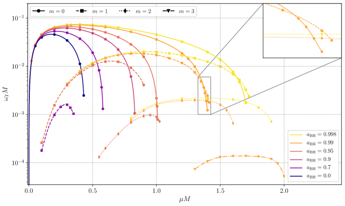
Figure 1: The growth rates $\omega_{I}$ of linear massive spin-2 field perturbations propagating in a Kerr background spacetime of mass $M$ and dimensionless spin $a_{\rm BH}$, characterized by their azimuthal mode number $m$, as a function of the mass parameter $\mu$. Data points indicate the rates extracted from our time-domain evolutions (available at Ref. spi ), while the lines connecting the points are cubic interpolations.

We begin by studying the linear stability of massive spin-2 perturbations on a Kerr BH background, which is generically governed by Eq. (1). In Refs. Babichev and Fabbri (2013); Brito et al. (2013a), it was noted that Schwarzschild BHs are unstable to a monopolar instability ($m=0$) with purely imaginary frequency: $\omega_{I}\sim\mu$. Kerr BHs are unstable to the growth of $m>0$ superradiant massive spin-2 modes, as shown in Ref. Brito et al. (2013a, 2020); Dias et al. (2023a). The fastest growing dipolar ($m=1$) mode was identified perturbatively in the $\alpha\ll 1$ regime, with scaling $\omega_{I}M\sim\alpha^{3}$, while $\omega_{I}M\sim\alpha^{2m+5}$ for $m\geq 2$ in this regime. Hence, the monopolar instability should dominate in the $\alpha\ll 1$ limit. Therefore, a natural question arises: where in the parameter space is the monopolar instability the fastest?

To address this question, we extend these analyses by considering (i) the monopolar instability on a Kerr background spacetime up to $a_{\rm BH}=0.998$, (ii) the most unstable dipolar superradiant family of modes in the highly relativistic limit of the parameter space, and (iii) higher-order unstable modes of the spin-2 field with $m=2$ and $m=3$. In Fig. 1, we compare the growth rates $\omega_{I}$ of all these modes across the relevant parameter space, obtained using the methods outlined in Sec. II (with details in Appendix A).

Focusing on the monopolar modes first, the growth rates follow the spin-independent scaling $\omega_{I}\approx 0.62\mu$ in the $\alpha\ll 1$ regime. These unstable modes turn stable at a critical mass $\mu_{c}$. This critical point goes from $\mu_{c}M\approx 0.44$ in the Schwarzschild case (which is consistent with Ref. Brito et al. (2013a)) up to $\mu_{c}M\approx 1.73$ for $a_{\rm BH}=0.998$, near the extremal limit. The maximum of the monopolar instability rate surpasses the rate of the slowest decaying quasinormal mode of the BH when $a_{\rm BH}\gtrsim 0.91$. The $m\geq 1$ superradiant modes exhibit the expected scaling in the $\alpha\ll 1$ limit Brito et al. (2020), and show good agreement with the results in Ref. Dias et al. (2023a) in the region of overlap. (See Appendix C for a detailed comparison to Refs. Brito et al. (2020); Dias et al. (2023a), including the values of $\omega_{R}$.) In the $\alpha\sim\mathcal{O}(1)$ regions of the parameter space, these modes turn stable when the superradiance condition is saturated $\omega_{R}=m\Omega_{H}$ (where $\Omega_{H}$ is the BH horizon frequency).

Comparing the monopolar ($m=0$) mode with the most unstable superradiant $m=1$ mode, it becomes clear from Fig. 1 that the monopolar instability dominates the dynamics of the system in the linear regime across large ranges of the relevant parameter space. In fact, only in the near-extremal limit, for critical spin of $a^{c}_{\rm BH}>0.95$, are the growth rates of the most unstable $m=1$ superradiant configuration comparable or larger than those of the monopolar instability. (For comparison, we note that if instead one assumed that the value of the critical mass for the monopolar mode remained roughly constant with black hole spin at the Schwarzschild value of $\mu_{c}M\approx 0.44$, this would give a critical spin of $a^{c}_{\rm BH}\sim 0.72$ for the $m=1$ superradiant instability to dominate Dias et al. (2023a).)

Considering higher order superradiant modes, this critical spin reduces with increasing azimuthal index $m$. From Fig. 1, $a^{c}_{\rm BH}<0.95$ for the $m=2$ superradiantly unstable configurations and $a^{c}_{\rm BH}\sim 0.7$ for $m=3$. Note, however, the maximum growth rate at fixed spin decreases roughly exponentially with increasing azimuthal index.

IV Nonlinear evolution

The results in the previous section indicate that the $m=0$ instability is the fastest growing massive tensor mode around a Kerr BH for much of the parameter space, leading naturally to the question: what is the nonlinear development of this instability? Due to the connection with the Gregory-Laflamme instability Gregory and Laflamme (1993) and questions of cosmic censorship Lehner and Pretorius (2010); Figueras et al. (2023), this of theoretical, in addition to phenomenological interest. The answer will in general depend on the particular nonlinear model chosen, and will not be fully addressed here. However, to gain some insight into the possibilities, we will consider nonlinear evolutions in Einstein-Weyl gravity, restricting to axisymmetry.

To begin with, we note a peculiarity of this theory is that, since the linearly growing tensor field is just the (trace-free) Ricci tensor $R_{ab}$, if we think of the backreaction on the BH metric as occurring through an effective stress-energy tensor, in this case this would just be proportional to $R_{ab}$ itself, and hence linearly (and not quadratically) dependent on the exponentially growing mode. Hence, for any set of parameters, we find two possible types of nonlinear behavior depending on the initial sign of the perturbation: one corresponding to the BH mass decreasing at the expense of the growing massive tensor field, and the other corresponding to the BH mass growing.

First considering nonspinning BHs, in Fig. 2, we illustrate the evolution of the BH mass as a result of the spherically symmetric instability for different values of $\alpha$. When the BH mass grows, the instability eventually saturates with the development of a massive tensor cloud of effectively negative energy, and a BH mass exceeding the value where the instability shutoffs for the isolated case: $M_{\rm BH}\gtrsim 0.44/\mu$. However, when the value of $\alpha$ is much smaller than this, the BH mass can significantly overshoot this threshold before saturating, e.g. by $\approx 30\%$ for $\alpha=0.05$.

In contrast, when the BH mass decreases, we find no evidence for a saturation of the instability, and the BH mass appears to approach zero in finite time (though, of course, at finite numerical resolution we are not able to track the decrease to arbitrarily small values). In the bottom panel of Fig. 2, we show a case where (through the use of high resolution) we track the BH as its mass decreases by a factor of $\approx 40$, and find that it roughly follows $M_{\rm BH}\propto(t-t_{0})$ (in harmonic time) at late times. We expect the curvature at the horizon to diverge as the BH becomes arbitrarily small since $R_{abcd}R^{abcd}=0.75M_{\rm BH}^{-4}$ at the horizon of a Schwarzschild BH. As shown in Fig. 2, we indeed find that the curvature outside the shrinking apparent horizon blows up in this way, suggesting that the end state will be a naked curvature singularity.

At the linear level, when $M_{\rm BH}\ll 1/\mu$, the instability rate is independent of the BH mass, i.e., $\omega_{I}\sim\mu$, and thus the instability timescale becomes long compared to the dynamical timescale of the BH. If one naïvely assumes (in analogy to the superradiance instability of spin-0 and spin-1 fields) that in the nonlinear regime of the instability the spacetime migrates through a sequence of quasi-stationary Schwarzschild BHs of adiabatically varying mass, then this finite-time diverging behavior is expected purely from the linear analysis. Since when $M_{\rm BH}\ll 1/\mu$, $\dot{M}_{\rm BH}=-\dot{M_{c}}=-C\mu M_{c}$ where $C$ is a numerical constant independent of the BH mass $M_{\rm BH}$ and cloud mass $M_{c}$, in this adiabatic approximation the BH’s mass decreases to zero in finite time roughly as

$$M_{\rm BH}\approx M_{\rm BH}^{t=0}+M_{c}^{t=0}(1-e^{C\mu t})\ .$$ (5)

Expanding this expression around the time $t_{0}$ when $M_{\rm BH}=0$ gives $M_{\rm BH}\propto(t-t_{0})$, as found in the Einstein-Weyl evolutions. This means that generically a nonlinear theory must exhibit some strong backreaction at small scales in order for black holes to avoid the fate found here.

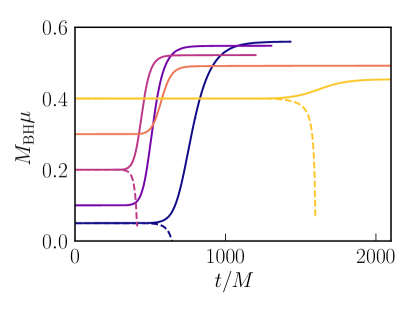
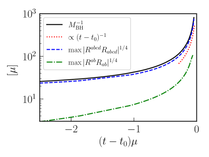
Figure 2: Top: the BH mass as a function of time during the nonlinear development of the spherically symmetric instability in Einstein-Weyl gravity for different values of $\alpha=\mu M$ from 0.05 to 0.4. Solid lines indicate unstable modes that cause the BH mass to grow, eventually saturating with clouds of the massive tensor field surrounding them. Corresponding dashed lines indicate opposite sign modes (with the same linear instability rate) that cause the BH mass to shrink to zero as far as the evolution can be carried out. Bottom: the late-time development of the instability where the BH shrinks for $\alpha=0.05$. The BH mass appears to approach zero at time $t_{0}$ linearly in harmonic time, with the maximum value of $|R_{abcd}R^{abcd}|$ outside the apparent horizon blowing up like $M_{\rm BH}^{-4}$. The Ricci tensor squared $R_{ab}R^{ab}$ is subdominant, but its maximum magnitude also increases at a similar rate.

Next, we consider the axisymmetric instability of spinning BHs. For simplicity, we fix $\alpha=0.4$ and vary the initial value of $a_{\rm BH}$. The resulting evolution of the BH mass and angular momentum is shown in Fig. 3. For the sign of the initial perturbation where the BH mass decreases, we find that the spin decreases as well (in this theory, the massive tensor degree of freedom can carry away angular momentum even in axisymmetry), rapidly approaching zero. Thus, we expect that these cases will behave similarly to the case without angular momentum, approaching a zero-mass, nonspinning BH in finite time. In contrast, for the opposite sign perturbation, the BH mass and spin both increase. For smaller initial spins, we again find that the solutions eventually saturate with a larger mass BH surrounded by a massive tensor cloud. However, for larger initial spins, we find that the mass and angular momentum rapidly increase, with the latter reaching super-extremal values: $J_{\rm BH}>A_{\rm BH}/(8\pi)$ (note that, by construction, $J_{\rm BH}\leq M_{\rm BH}^{2}$) Booth and Fairhurst (2008). In these cases, our evolutions eventually breakdown (primarily due to not being able to track the apparent horizon), and we leave the question of the ultimate fate of these cases to future work.

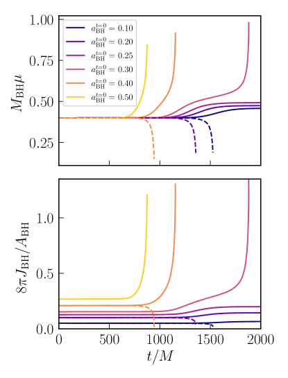
Figure 3: The nonlinear development of the axisymmetric ($m=0$) instability of BHs in Einstein-Weyl gravity for $\alpha=0.4$ and different initial values of the dimensionless BH spin $a_{\rm BH}\in[0.1,0.5]$. We show the evolution of the BH mass (top panel) and angular momentum normalized by the apparent horizon area (bottom panel), with the same color used in both panels for each case. Solid lines indicate unstable modes that cause the BH mass and spin to grow. The lower spin cases saturate, as in the nonspinning cases. However, the higher spin cases exhibit rapidly increasing masses, and violate the extremality bound $J_{\rm BH}\leq A_{\rm BH}/(8\pi)$, and we are eventually unable to continue the evolution. Corresponding dashed lines indicate select cases with opposite sign modes that cause the BH spin and mass to decrease toward zero, in a similar manner to the nonspinning cases shown in Fig. 2.

Here, we have restricted our spacetime to be axisymmetric ($m=0$), precluding the effect of the superradiant instability. However, we do not expect this restriction to significantly affect the cases we consider as the superradiant instability would operate on much longer timescales than considered here. For the spinning cases we study, when the massive spin-2 cloud grows with positive energy, it rapidly spins down the black hole, making superradiance irrelevant; when the massive spin-2 cloud grows with negative energy, the black hole either rapidly reaches a super-extremal state where we can no longer follow it, or it saturates at a moderate spin where (assuming the instability rates are roughly comparable to the equivalent values in Kerr) superradiance would be slow.

V Discussion and Conclusion

Using time domain evolutions to study the linear regime of theories propagating a massive tensor on the background of a spinning BH, we find that the monopolar instability dominates over the superradiant instability in much of the parameter space. Therefore, one cannot use the latter to place constraints on massive spin-2 fields without taking into account the backreaction of the former. Note that, for $\alpha\ll 1$, the monopolar instability always dominates, regardless of the BH spin, and has a timescale that is independent of the BH’s mass Babichev and Fabbri (2013); Brito et al. (2013a), $\tau_{\rm mono.}\approx 10\ \text{s}\ (10^{-16}\ \text{eV}/{m_{b}})$. As a result, all BHs, from solar-mass to supermassive ones with $M_{\rm BH}=10^{10}M_{\odot}$, are unstable to the monopolar instability with timescales smaller than the Salpeter accretion time: $\tau_{\rm mono.}<4.5\times 10^{7}\ \text{yrs}$, for a spin-2 field of mass $6\times 10^{-21}\ {\rm eV}>m_{b}>7\times 10^{-31}$ eV. For spin-2 masses heavier than this, we find the superradiance instability becomes relevant in some parts of the parameter space with rapidly spinning BHs and $\alpha\gtrsim\mathcal{O}(1)$. Finally, for $m_{b}\gtrsim 5\times 10^{-11}$ eV, even a light BH of mass $5\ M_{\odot}$ is stable to monopolar modes, but may be unstable to superradiant modes with higher azimuthal numbers. We also find that higher azimuthal numbers are required for the superradiant instability to be relevant at moderately high spins (e.g. $m\geq 3$ for $a_{\rm BH}\lesssim 0.7$, as typical for the remnant of a low-spin, quasicircular binary BH merger). Hence, an interesting direction for future work is to determine the growth rates for these more precisely.

As a simple model of the backreaction of the $m=0$ instability, we carry out evolutions in Einstein-Weyl gravity. Though the backreaction will be different in other (and in particular, ghost-free) nonlinear theories, there are several features that we find that can already be anticipated from the linear theory, and thus may be more generic. Due to the short timescales, we find that the BH can noticeably overshoot the values where the linear analysis, considering the BH in isolation, would indicate the instability shuts off. This contrasts with the spin-1 (and presumably spin-0) superradiant instability, where the timescales are longer East and Pretorius (2017); East (2018). This overshooting happens when the BH mass grows to a larger value with a surrounding ghost spin-2 field cloud, and the instability saturates outside the regime where the linear analysis would indicate the superradiant instability is active. On the other hand, when the spin-2 field grows at the expense of decreasing the BH mass (as one would also expect for a nonghost field), this leads the BH to approach zero mass in finite time. This is consistent with the fact that, in the limit of small BH mass, the linear instability rate has a nonzero value $\sim\mu$. Notably, the Gregory-Laflamme instability of a black string Gregory and Laflamme (1993), which has the same linear structure as the monopolar instability, also has a similar fate: points along the black string shrink to zero radius in finite time, also leading to a mild, zero-mass, naked curvature singularity Lehner and Pretorius (2010); Figueras et al. (2023). This type of singularity is also what arises in critical gravitational collapse Choptuik (1993).

For future work, it would be interesting to study the development of the monopolar BH instability in other nonlinear theories, as well as to better understand the fate of the BHs that we found to be spun up to extremal values by the instability. One might also expect BHs to be spun up in theories where the instability decreases the BH mass without extracting significant angular momentum. It would also be interesting to follow the nonlinear development of the superradiant instability in the regimes identified here where it dominates. Of particular observational importance is the (likely model-dependent) question of the gravitational wave signatures of these different instabilities. A theory propagating both a massive and a massless spin-2 field has, in general, more than two gravitational wave polarization states with nontrivial dispersion relations Bogdanos et al. (2010); Tachinami et al. (2021), which gravitational wave detectors could, in principle, be sensitive to.

Appendix A Evolution Equations and Numerical Scheme

For the linear massive tensor field evolutions, we numerically evolve $H_{ab}$ and $\partial_{t}H_{ab}$ according to Eq. (1) on the background of a Kerr BH. As in harmonic and Z4 formulations of general relativity Gundlach et al. (2005), we find it necessary in BH spacetimes to add additional terms to Eq. (1) that serve to damp violations of the constraint $\nabla_{a}H^{ab}=0$:

$$\Box H_{ab}= \mu^{2}H_{ab}-2R_{acbd}H^{cd}$$

$$- \kappa\left(n_{a}\nabla^{c}H_{bc}+n_{b}\nabla^{c}H_{ac}-\frac{1}{2}g_{ab}n^{c}\nabla^{d}H_{cd}\right)\ .$$ (6)

The terms on the second line will converge to zero as $\nabla_{a}H^{ab}\rightarrow 0$, but serve to suppress constraint violating modes that might otherwise grow, damping them on a timescale $1/\kappa$. In this study, we typically set $\kappa\sim 1/M_{\rm BH}$.

In order to consider different unstable modes in isolation, and to reduce the computational expense of the simulations, we consider cases where $H_{ab}$ has an azimuthal symmetry with azimuthal number $m$. Under this assumption, following Ref. East (2017), the computational domain can be reduced to two spatial dimensions by introducing, for book keeping purposes, an imaginary component to the massive tensor, $H_{ab}=H^{R}_{ab}+iH^{I}_{ab}$, and requiring that $\mathcal{L}_{\phi}H_{ab}=imH_{ab}$, where $\mathcal{L}_{\phi}$ is the Lie derivative with respect to the axisymmetric Killing vector. We use Cartesian coordinates, but restrict our domain to the half plane with $0\leq x<\infty$, $y=0$, and $-\infty<z<\infty$. By evolving both the real and imaginary part of $H_{ab}$ according to Eq. (6), we can compute out-of-plane derivatives $\partial_{y}H_{ab}$ using the symmetry assumption. On the symmetry axis, we apply regularity conditions to the components of $H_{ab}$. These expressions were obtained following the procedure in appendix A of Ref. Pretorius (2005).

For the nonlinear evolutions in Einstein-Weyl gravity, our evolution variables are $\{g_{ab},\partial_{t}g_{ab},R_{ab},\partial_{t}R_{ab}\}$. Following Ref. Noakes (1983), the metric is evolved in the generalized harmonic formulation, where the gauge degrees are freedom are fixed by requiring that $\Box x^{a}=H^{a}$, where $H^{a}$ are specified functions of the metric. The only difference is that $R_{ab}$ now acts as a source term when evolving the metric:

$$g^{cd}\partial_{c}\partial_{d}g_{ab}=-2\nabla_{(a}H_{b)}+2H_{c}\Gamma^{c}_{ab}-2\Gamma^{c}_{da}\Gamma^{d}_{cb}$$

$$-\kappa\left(n_{a}C_{b}+n_{b}C_{a}-n_{c}C^{c}g_{ab}\right)$$

$$-2\partial_{c}g_{d(a}\partial_{b)}g^{cd}-2R_{ab},$$ (7)

where we have also included the usual terms to damp the generalized harmonic constraint $C^{a}=H^{a}-\Box x^{a}$  Gundlach et al. (2005).

The Ricci tensor is evolved according to Eq. (4), but with the addition of the same constraint damping term as in Eq. (6). The Riemann tensor term in Eq. (4) is calculated from the metric and its derivatives, but with the second time derivatives of $g_{ab}$ being determined by substituting in Eq. (7). Recall that, under our assumptions, $R_{a}^{a}=0$. We evolve all ten components of $R_{ab}$, but subtract out any trace component (due to truncation error) at each time step. See Refs. Held and Lim (2021, 2023) for related evolution schemes.

For the linear evolutions, we use either harmonic coordinates Cook and Scheel (1997) or (when the BH spin is large) Cartesian Kerr-Schild coordinates Kerr and Schild (1965). For the nonlinear evolutions, we begin with a BH in harmonic coordinates and use the harmonic gauge: $\Box x^{a}=0$. Spatial derivatives are discretized using fourth-order finite difference stencils, while time stepping is performed using fourth-order Runge Kutta. We use adaptive mesh refinement to concentrate numerical resolution around the BH, but the interpolation for the refinement boundaries is only accurate to third-order in the size of the time step.

For the nonlinear evolutions in axisymmetry, we track the BH apparent horizon by finding the outermost marginally outer trapped surface using a flow method Pretorius (2005). Integrating over the horizon surface, we compute the area $A_{\rm BH}$, and the angular momentum

$$J_{\rm BH}=\frac{1}{8\pi}\int\hat{\phi}_{i}K^{ij}dA_{j}\ ,$$ (8)

where $K^{ij}$ is the extrinsic curvature and $\hat{\phi}^{i}$ is the axisymmetric Killing vector. From these quantities we can define a BH mass through the Christodoulou formula

$$M_{\rm BH}:=\left(\frac{A_{\rm BH}}{16\pi}+\frac{4\pi J_{\rm BH}^{2}}{A_{\rm BH}}\right)^{1/2}\ .$$ (9)

Note that, with this definition, the dimensionless spin is given by

$$a_{\rm BH}=\frac{J_{\rm BH}}{M_{\rm BH}^{2}}=\frac{2j}{1+j^{2}}\ {\rm with}\ j=\frac{8\pi J_{\rm BH}}{A_{\rm BH}}.$$ (10)

Hence, $a_{\rm BH}$ obtains a maximum of $a_{\rm BH}=1$ at $j=1$ and decreases for larger $j$.

Appendix B Numerical Convergence

For most of the evolutions we perform, we use a computational domain with seven or eight levels of mesh refinement centered on the BH, and where the grid spacing on the finest level is between $dx\approx 0.04M$ and $0.02M$. For nonlinear evolutions where the BH shrinks, we add additional resolution and mesh refinement levels. In the most extreme case, shown in the bottom panel of Fig. 2, we have $dx\approx 5\times 10^{-4}M$ on the finest level used. We also perform resolution studies of select cases to check for convergence and to estimate numerical errors.

In Fig. 4, we show a norm of the Bianchi constraint violation $\sum_{b}|\nabla_{a}H^{ab}|/4$, integrated over the domain, during a linear evolution case with $m=1$ (summing the contributions from the real and imaginary components). We normalize this quantity by the norm of the massive tensor $|H^{ab}H_{ab}|$, as the whole solution is exponentially increasing due to the instability. As evident from the figure, the relative constraint violation at later times is roughly constant in time, and converging to zero with increasing resolution. We show a nonlinear evolution with Einstein-Weyl gravity in Fig. 5. There, in addition to the Bianchi constraint violation, we show the norm of the generalized harmonic constraint. As can be seen from the plot, the constraints converge to zero with increasing resolution at the expected rate (between third and fourth order).

Figure 4: The evolution of the Bianchi constraints $\mathcal{I}_{C}:=\int d^{3}x[\sum_{a}(\nabla_{b}H^{ab}_{R})^{2}]^{1/2}+(R\leftrightarrow I)$, normalized by the field amplitude $\mathcal{I}_{H}:=|\int d^{3}xH_{ab}^{R}H^{ab}_{R}|^{1/2}+(R\leftrightarrow I)$, throughout the development of the $m=1$ superradiance instability of a massive spin-2 field on a Kerr BH background with spin $a_{\rm BH}=0.95$ and $\alpha=0.7$. Since the initial perturbation used to trigger the linear instability does not satisfy the constraints, they do not converge at early times. At later times, both $\mathcal{I}_{C}$ and $\mathcal{I}_{H}$ grow exponentially at the instability rate. The different resolutions have been scaled by a factor consistent with fourth order convergence.

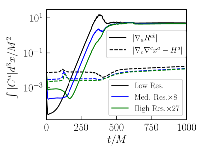
Figure 5: The convergence of the constraints with increasing resolution for a nonlinear evolution in Einstein-Weyl gravity of a nonspinning BH with $\alpha=0.2$. In this case (corresponding to the solid magenta curve in Fig. 2), the BH mass increases and saturates at a larger value. We show both the norm of the Bianchi constraint $\nabla_{a}R^{ab}=0$ (solid lines) and the generalized harmonic constraint $H^{a}-\Box x^{a}=0$ (dashed lines) integrated on the domain. The constraints converge at between third and fourth order, with the different resolutions scaled by a factor consistent with the former. Due to the fact that the initial perturbation we use does not satisfy the constraints, there is nonconvergence in the Bianchi constraint at early times, but this is exponentially small compared to the subsequent truncation error, and does not affect the convergence at later times.

For several of the linear evolutions cases, we extract the instability growth rate at three different resolutions, and use Richardson extrapolation to estimate the truncation error in these quantity. The results are shown in Table 1. The errors in the instability rates for the default resolutions do vary noticeably with $\alpha$ for the considered values, ranging from order $10\%$ to a few percent or smaller, but these provide a rough estimate for the errors across the parameter space. Generally, we find that for larger BH spin and $\alpha$, the uncertainties are larger.

Table 1: A comparison of the instability growth rate measured at the default resolution, to the Richardson extrapolated value using three different resolutions. This gives a measure of the truncation error, shown as a percent in the last column.

			$M\omega_{I}$: default	Richardson	Error
$\alpha$	$a_{\rm BH}$	$m$	resolution	extrapolated version	(%)
0.4	0.99	0	$7.1872\times 10^{-2}$	$7.1866\times 10^{-2}$	0.01
1.6	0.998	0	$7.65\times 10^{-3}$	$8.07\times 10^{-3}$	5.2
0.7	0.95	1	$1.27\times 10^{-2}$	$1.25\times 10^{-2}$	1.6
0.9	0.998	1	$1.91\times 10^{-2}$	$2.01\times 10^{-2}$	5.0
1.0	0.95	2	$8.80\times 10^{-4}$	$8.18\times 10^{-4}$	8.0
1.5	0.99	2	$1.59\times 10^{-3}$	$1.40\times 10^{-3}$	14
1.4	0.998	2	$2.19\times 10^{-3}$	$2.13\times 10^{-3}$	3.0
1.9	0.99	3	$1.19\times 10^{-4}$	$1.08\times 10^{-4}$	10

Appendix C Real frequencies and comparison to literature

For completeness, we provide the real parts of the frequencies associated with the fastest growing $m=1$ and $m=2$ superradiant modes (the $m=0$ modes have zero real frequency) here, and compare these, as well as the growth rates, to results obtained in Refs. Dias et al. (2023a); Brito et al. (2020). To that end, we show the real parts of the frequencies in Fig. 6 and the imaginary parts in Fig. 7.

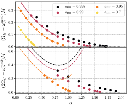
Figure 6: The real part of the frequency $\omega_{R}$ of the most unstable $m=1$ (top) and $m=2$ (bottom) superradiant modes of a massive spin-2 field around Kerr BHs of various dimensionless spins $a_{\rm BH}$. Circular points correspond to our time-domain results. The dashed lines are interpolations of the numerical results in Ref. Dias et al. (2023a), for the most unstable $m=1$ mode, and analytic expressions determined in Ref. Brito et al. (2020), for the most unstable $m=2$ superradiant state.

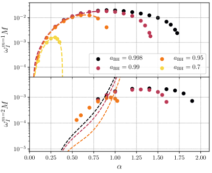
Figure 7: The top and bottom panels correspond to the imaginary part of the frequency $\omega_{I}$ of the $m=1$ and $2$ modes, respectively, shown in Fig. 6 (circular points). For comparison, we show the interpolated numerical data from Ref. Dias et al. (2023a) (top) and the analytic expressions from Ref. Brito et al. (2020) (bottom) for these unstable modes (dashed lines).

In Ref. Dias et al. (2023a), the frequencies, $\omega_{R}$ and $\omega_{I}$, of the most unstable $m=1$ superradiant modes were determined by solving the elliptic equations governing the eigenvalue problem for $\alpha\leq 0.8$ and $a_{\rm BH}\leq 0.99$. Comparing their results (interpolated to some of the specific values of $a_{\rm BH}$ we consider) in the region where they overlap with ours in the top panels of Figs. 6 and 7, we find good agreement (to within roughly $5\%$, and consistent with the expected truncation error).

In Ref. Brito et al. (2020), analytic estimates for $\omega_{R}$ and $\omega_{I}$ of the most unstable $m=2$ superradiant modes were obtained in the $\alpha\ll 1$ limit. Up to $\alpha\approx 0.5$, these expressions for $\omega_{R}$ match our results (compare, in particular, the $m=2$ and $a_{\rm BH}=0.95$ family of modes in Fig. 6). The estimates for the growth rates of these configurations, on the other hand, are inconsistent with our time-domain predictions at $\alpha\approx 0.5$; we expect that the agreement would be better in the $\alpha<0.5$ region of the parameter space. Our data for the $m=3$ superradiant mode covers $\alpha\geq 1.3$, a regime in which we do not find good agreement with the perturbative estimates valid in the $\alpha\ll 1$ limit.

Finally, we mention that the numerical values of $\omega_{R}$ and $\omega_{I}$ calculated in this work for $m=0$, 1, 2, and 3 (as well as some lower values of $a_{\rm BH}$ for $m=0$ omitted here for clarity) are available at Ref. spi .