A Stiff Pre-CMB Era with a Mildly Blue-tilted Tensor Inflationary Era can Explain the 2023 NANOGrav Signal

Abstract

We examine the effects of a stiff pre-recombination era on the present day’s energy spectrum of the primordial gravitational waves. If the background total equation of state parameter at the pre-recombination era is described by a kination era one, this directly affects the modes with characteristic wavenumbers which reenter the Hubble horizon during this stiff era. The stiff era causes a broken-power-law effect on the energy spectrum of the gravitational waves. We use two approaches, one model agnostic and a specific model that can realize this scenario. In all cases, the inflationary era can be realized either by some theory leading to a standard red-tilted tensor spectral index or by some theory which has a mild tensor spectral index $n_{\mathcal{T}}=0.17-0.37$ like an Einstein-Gauss-Bonnet theory. For the model agnostic scenario case, the NANOGrav signal can be explained by the stiff pre-recombination era combined with an inflationary era with a mild blue-tilted tensor spectral index $n_{\mathcal{T}}=0.37$ and a low-reheating temperature $T_{R}\sim 0.1$GeV. In the same case, the red-tilted inflationary theory signal can be detectable by the future LISA, BBO and DECIGO experiments. The model dependent approach is based on a Higgs-axion model which can yield multiple deformations of the background total equation of state parameter, causing multiple broken-power-law behaviors occurring in various eras before and after the recombination era. In this case, the NANOGrav signal is explained by this model in conjunction with an inflationary era with a really mild blue-tilted tensor spectral index $n_{\mathcal{T}}=0.17$ and a low-reheating temperature $T_{R}\sim 20\,$GeV. In this case, the signal can be detectable by the future Litebird experiment, which is a very characteristic pattern in the tail of the primordial gravitational wave energy spectrum.

I Introduction

Inflation [1, 2, 3, 4] is now put to test from most current and forthcoming experiments. The aim is to pinpoint the B-modes directly experimentally, and this is the central focus of the stage 4 Cosmic Microwave Background (CMB) experiments [5, 6]. Apart from the B-modes, there are indirect ways to detect an inflationary era, for example the detection of a small (or negligible) anisotropy stochastic gravitational wave background [7, 8, 9, 10, 11, 12, 13, 14, 15]. These future gravitational wave experiments will directly probe the inflationary tensor perturbations. Apart from the LIGO-Virgo successes and exciting observations, recently the NANOGrav collaboration confirmed the well anticipated stochastic gravitational wave detection [16], which was also confirmed by other pulsar timing arrays (PTA) experiments [17, 18, 19]. The scientific community was almost certain that the 2020 signal detection was not due to the actual pulsar red noise but due to a stochastic gravitational wave background, which was confirmed in 2023 due to the presence of Hellings-Downs correlations. After the 2023 NANOGrav announcement, a large stream of research articles were produced, trying to explain the signal, for the cosmological perspective see for example [20, 21, 22, 23, 24, 25, 26, 27, 28, 29, 30, 31, 32, 33, 34, 35, 36, 37, 38, 39, 40, 41, 42, 43, 44, 45, 46, 47, 48, 49, 50, 51, 52, 53, 54, 55, 56, 57, 58, 59, 60, 61, 62, 63, 64], see also [65, 66, 67, 68, 69, 70, 71] for earlier works in this perspective, and also [24, 25, 72] for the axion description. Although it is not certain whether the 2023 NANOGrav signal has a cosmological or astrophysical source, or even a combination of the two, there are theoretical hints toward the cosmological description. For the astrophysical description of the signal, see the recent review [73]. Currently there are some issues that render the cosmological description more plausible, although in principle the signal may be a hybrid of astrophysical and cosmological origin. The obstacles for the astrophysical description are firstly the lack of a concrete solution for the last parsec problem [74], secondly, the absence of large anisotropies in the NANOGrav signal [75] and thirdly the complete absence of isolated supermassive black hole merger events. Clearly, the detection of large anisotropies in the future may point out that the astrophysical description is plausible [76, 77]. However, some hint in this direction should be present even in the 2023 data, so the near future will shed light on these issues. On the other hand, there are a lot of cosmological scenarios that may explain the signal, like phase transitions, cosmic strings, primordial black holes and so on. With regard to the inflationary perspective, it seems that ordinary inflation cannot explain in any way the 2023 NANOGrav signal, unless a highly blue-tilted tensor spectral index is produced and a significantly low-reheating temperature is required [20, 21, 78, 79]. In principle, a blue-tilted tensor spectral index can be generated in the context of many theories, like string gas theories [80, 81, 82], or some Loop Quantum Cosmology scenarios can also predict such a tensor spectrum [83, 84, 85, 86], and moreover the non-local version of Starobinsky inflation [87, 88, 89] which also yield an acceptable amount of non-Gaussianities. Furthermore, it is important to note that conformal field theory can yield a blue-tilted tensor spectrum [90], see also [91] for a different perspective. From the aforementioned examples, the only which yields a strongly blue-tilted tensor spectral index is the non-local Starobinsky model, however in such a case a low reheating temperature is also needed. In the case that the reheating temperature is actually too low, the electroweak phase transition is put into peril, since it cannot be realized thermally, it is required that the reheating temperature is at least 100 GeV. We shall discuss this important issue at a later section. Thus the situation is somewhat perplexed since it is not certain what causes the 2023 NANOGrav signal. Only the combination of data coming from all the future experiments like LISA and the Einstein Telescope, including NANOGrav, may point out toward to a specific model behind the stochastic signal. This synergy between experiments may also help determining the reheating temperature.

In view of the above line of research, in this work we shall report an intriguing result in the context of inflationary theories and their ability to explain the 2023 NANOGrav signal. Our analysis requires a stiff, or nearly stiff pre-CMB era, which can be caused by various mechanisms, see for example [92, 93, 94, 95, 96, 97, 98, 99, 100, 101, 94]. The approach of Ref. [92] remarkably fits the line of research we shall adopt in this work, and the pre-CMB stiff or kination era is caused by the axion. Actually the authors perform a thorough and scientifically sound analysis to put constraints on such a pre-CMB kination era caused by the axion. We shall not use a specific model in our work, however the constraints of [92] are taken into account in our analysis. In a previous work we considered the effects of stiff eras caused by axions during reheating [95], so this work is basically in the same spirit as our previous one. Also it is noticeable that recently another work which invokes a stiff era and the possibility of explaining the NANOGrav 2023 signal appeared in the literature [102], in a different approach though, compared to the one we shall present in this work. Coming back to our case, the stiff era is required to correspond at a wavenumber range $k=0.4-0.9\,$Mpc^-1, so just before the recombination era, and recall that the CMB pivot scale is at $k=0.002$ Mpc^-1. Note that the CMB modes with $k=0.002$ Mpc^-1 reentered the horizon at $z=1100$ so during recombination, so the stiff era is assumed to have occurred before the recombination so when $k=[0.4,0.9]\,$Mpc^-1 hence for a redshift $2500>z>1100$ and and well below the matter-radiation redshift. The inflationary era can be described by a standard red-tilted or a blue-tilted theory. With regard to the red-tilted inflationary era, it can be described by a standard inflationary scenario or some modified gravity [103, 104, 105, 106, 107, 108, 109], while the blue-tilted inflationary era can be described for example by an Einstein-Gauss-Bonnet gravity. The striking new result is that the tensor spectral index in the latter case is not required to be strongly blue-tilted, but it can be of the order $\sim\mathcal{O}(0.37)$, which can be easily generated by an Einstein-Gauss-Bonnet theory. In the case of a blue-tilted inflationary era, the compatibility with the NANOGrav result comes easily when the reheating temperature is of the order $T\sim\mathcal{O}(0.1)\,$GeV, while the red-tilted inflationary case scenario is not detectable by the NANOGrav, however the prediction is that can be either detected by LISA or by the Einstein Telescope, not simultaneously though, depending on the reheating temperature and the total equation of state (EoS) parameter post-inflationary.

Regarding the stiff pre-CMB era, we shall assume an agnostic approach without proposing a model for this, except for the last section where we shall discuss a potentially interesting model.

II Stiff Pre-CMB era, Standard or Blue-tilted Inflation and Gravitational Waves

Apparently, after the recent successes in gravitational wave detections, the interest of theoretical physicists and cosmologists is focused on gravitational waves and specifically those having primordial origin. In the literature there exist several works on primordial gravitational waves, for a mainstream of research articles and reviews see [110, 111, 112, 113, 114, 115, 116, 117, 118, 79, 119, 120, 121, 122, 123, 124, 125, 126, 127, 128, 129, 130, 131, 132, 133, 134, 135, 136, 137, 138, 139, 140, 141, 142, 143, 144, 145, 146, 147, 148, 149, 150, 151, 152, 153] and the recent review Ref. [154].

Before getting to the core of this work, it is worth recalling the expression for the energy spectrum of the primordial gravitational waves for the general relativistic case, assuming a primordial inflationary era and a dark energy late-time era. We shall consider a spatially flat Friedmann-Robertson-Walker (FRW) background with metric,

$$\centering{\rm d}s^{2}=-{\rm d}t^{2}+a(t)^{2}\sum_{i=1}^{3}{({\rm d}x^{i})^{2}}\,,\@add@centering$$ (1)

with $a(t)$ denoting the scale factor and $t$ stands for the cosmic time. Since we are interested in inflationary originating gravitational waves, we shall use the conformal time $\tau$, with the FRW line element written in this case as follows,

$${\rm d}s^{2}=a^{2}[-{\rm d}\tau^{2}+(\delta_{ij}+h_{ij}){\rm d}x^{i}{\rm d}x^{j}],$$ (2)

and the $x^{i}$ stand for the comoving spatial coordinates, while the tensor $h_{ij}$ denotes the gauge-invariant tensor perturbation of the metric, which is symmetric ($h_{ij}\!=\!h_{ji}$), traceless $h_{ii}\!=\!0$, and transverse $\partial^{j}h_{ij}\!=\!0$. Now if the tensor perturbation is considered as a quantum field $h_{ij}(\tau,{\bf x})$ as a quantum field in the unperturbed FRW spacetime $g_{\mu\nu}=diag\{-a^{2},a^{2},a^{2},a^{2}\}$, we can construct the second order quadratic action of the tensor perturbations,

$$S=\int d\tau d{\bf x}\sqrt{-g}\left[\frac{-g^{\mu\nu}}{64\pi G}\partial_{\mu}h_{ij}\partial_{\nu}h_{ij}+\frac{1}{2}\Pi_{ij}h_{ij}\right].$$ (3)

where $g^{\mu\nu}$ is the inverse of $g_{\mu\nu}$ and also $g$ denotes the determinant of the metric as usual. The tensor $\Pi_{\mu\nu}$ stands for the anisotropic stress $\Pi_{\mu\nu}$, which is defined as,

$$\Pi^{i}_{j}=T^{i}_{j}-p\delta^{i}_{j}$$ (4)

and also satisfies $\Pi_{ii}=0$ and also the transverse condition $\partial^{i}\Pi_{ij}=0$. Note that it is coupled to the metric tensor perturbation $h_{ij}$ and thus it acts as a source in the gravitational quantum action (3). By varying the gravitational quantum action (3) with respect to the $h_{ij}$, we obtain the evolution equation of the metric perturbation,

$$h_{ij}^{\prime\prime}+2\frac{a^{\prime}(\tau)}{a(\tau)}h_{ij}^{\prime}-{\bf\nabla}^{2}h_{ij}=16\pi Ga^{2}(\tau)\Pi_{ij}(\tau,{\bf x}),$$ (5)

with the prime denoting differentiation with respect to the conformal time $\tau$. Taking the fourier transformation of the evolution equation (5), we get,

$$h_{ij}(\tau,{\bf x})\!\! =\! \!\!\sum_{r}\sqrt{16\pi G}\!\!\int\!\!\!\frac{d{\bf k}}{(2\pi)^{3/2}}\epsilon_{ij}^{r}({\bf k})h_{{\bf k}}^{r}(\tau){\rm e}^{i{\bf k}{\bf x}},\qquad\quad$$ (6a)

$$\Pi_{ij}(\tau,{\bf x})\!\! =\! \!\!\sum_{r}\sqrt{16\pi G}\!\!\int\!\!\!\frac{d{\bf k}}{(2\pi)^{3/2}}\epsilon_{ij}^{r}({\bf k})\Pi_{{\bf k}}^{r}(\tau){\rm e}^{i{\bf k}{\bf x}},\qquad\quad$$ (6b)

with $r=$(“$+$” or “$\times$”) indicating the polarization of the gravitational tensor perturbation. The polarization tensors satisfy [$\epsilon_{ij}^{r}({\bf k})=\epsilon_{ji}^{r}({\bf k})$], and also are traceless $\epsilon_{ii}^{r}({\bf k})=0$, and transverse $k_{i}\epsilon_{ij}^{r}({\bf k})=0$. We shall choose a circular polarization basis satisfying $\epsilon_{ij}^{r}({\bf k})=(\epsilon_{ij}^{r}(\textrm{-}{\bf k}))^{\ast}$, so the polarization basis can be normalized as follows,

$$\sum_{i,j}\epsilon_{ij}^{r}({\bf k})(\epsilon_{ij}^{s}({\bf k}))^{\ast}=2\delta^{rs}.$$ (7)

Eq. (6) in conjunction with Eq. (3), yields,

$$S\!=\!\!\sum_{r}\!\!\int\!\!d\tau d{\bf k}\frac{a^{2}}{2}\;\!\!\Big{[}h_{{\bf k}}^{r}{}^{\prime}h_{\!\textrm{-}{\bf k}}^{r}\!{}^{\prime}\!-\!k^{2}h_{{\bf k}}^{r}h_{\!\textrm{-}{\bf k}}^{r}\!+\!32\pi Ga^{2}\Pi_{{\bf k}}^{r}h_{\!\textrm{-}{\bf k}}^{r}\Big{]}\,,$$ (8)

which is nothing but the tensor perturbations action (3), written in terms of the Fourier transformation of the metric perturbation. Now, imposing the canonical quantization conditions to the above action, using as a canonical configuration space variable the perturbation $h_{{\bf k}}^{r}$ and the conjugate momentum being,

$$\pi_{{\bf k}}^{r}(\tau)=a^{2}(\tau)h_{\!\textrm{-}{\bf k}}^{r}{}^{\prime}(\tau)\,,$$ (9)

therefore by making these quantum operators $\hat{h}_{{\bf k}}^{r}$ and $\hat{\pi}_{{\bf k}}^{r}$, the theory at hand can be quantized by using the following equal time commutation relation,

$$\left[\hat{h}_{{\bf k}}^{r}(\tau),\hat{\pi}_{{\bf k}^{\prime}}^{s}(\tau)\right] = i\delta^{rs}\delta^{(3)}({\bf k}-{\bf k}^{\prime}),$$ (10a)

$$\left[\hat{h}_{{\bf k}}^{r}(\tau),\hat{h}_{{\bf k}^{\prime}}^{s}(\tau)\right] = \left[\hat{\pi}_{{\bf k}}^{r}(\tau),\hat{\pi}_{{\bf k}^{\prime}}^{s}(\tau)\right]=0\,,$$ (10b)

and the Fourier components of $\hat{h}_{ij}(\tau,{\bf x})$ satisfy the following relation $\hat{h}_{{\bf k}}^{r}=\hat{h}_{\!\textrm{-}{\bf k}}^{r{\dagger}}$, since $\hat{h}_{ij}(\tau,{\bf x})$ is a Hermitian operator. Accordingly we have,

$$\hat{h}_{{\bf k}}^{r}(\tau)=h_{k}(\tau)\hat{a}_{{\bf k}}^{r}+h_{k}^{\ast}(\tau)\hat{a}_{\!\textrm{-}{\bf k}}^{r{\dagger}},$$ (11)

and the $\hat{a}_{{\bf k}}^{r{\dagger}}$ are the creation operators, while $\hat{a}_{{\bf k}}^{r}$ are the annihilation operators, which obey,

$$\Big{[}\hat{a}_{{\bf k}}^{r},\hat{a}_{{\bf k}^{\prime}}^{s{\dagger}}\Big{]} = \delta^{rs}\delta^{(3)}({\bf k}-{\bf k}^{\prime}),$$ (12a)

$$\Big{[}\hat{a}_{{\bf k}}^{r},\hat{a}_{{\bf k}^{\prime}}^{s}\Big{]} = \Big{[}\hat{a}_{{\bf k}}^{r{\dagger}},\hat{a}_{{\bf k}^{\prime}}^{s{\dagger}}\Big{]}=0\,.$$ (12b)

Note that the linearly-independent modes $h_{k}(\tau)$ and $h_{k}^{\ast}(\tau)$ satisfy the Fourier transformed evolution equation of the tensor perturbation,

$$h_{k}^{\prime\prime}+2\frac{a^{\prime}(\tau)}{a(\tau)}h_{k}^{\prime}+k^{2}h_{k}=16\pi Ga^{2}(\tau)\Pi_{k}(\tau).$$ (13)

By looking Eq. (11) it is obvious that the modes $h_{k}(\tau)$ have an explicit dependence on the conformal time and on the wavenumber $k=|{\bf k}|$. The Wronskian chronological past normalization condition,

$$h_{k}(\tau)h_{k}^{\ast}{}^{\prime}(\tau)-h_{k}^{\ast}(\tau)h_{k}^{\prime}(\tau)=\frac{i}{a^{2}(\tau)}$$ (14)

basically is the compatibility constraint between Eqs. (10) and (12). An essential feature of the standard approach for the primordial gravitational waves is the initial condition chosen for the Fourier mode of the tensor perturbation in the chronological past which assumes a Bunch-Davies initial vacuum state,

$$h_{k}(\tau)\to\frac{{\rm exp}(-ik\tau)}{a(\tau)\sqrt{2k}}\qquad({\rm as}\;\;\tau\to-\infty),$$ (15)

describing subhorizon modes $\vec{k}$ during inflation. Now let us proceed to the calculation of the energy spectrum of the gravitational waves $\Omega_{gw}(k,\tau)$, so an essential quantity is the $\Delta_{h}^{2}(k,\tau)$, which can be defined by the following,

$$\langle 0|\hat{h}_{ij}(\tau,{\bf x})\hat{h}_{ij}(\tau,{\bf x})|0\rangle\!=\!\!\!\int_{0}^{\infty}\!\!\!\!\!64\pi G\frac{k^{3}}{2\pi^{2}}\!\left|h_{k}(\tau)\right|^{2}\!\frac{dk}{k},$$ (16)

and is explicitly,

$$\Delta_{h}^{2}(k,\tau)\equiv\frac{d\langle 0|\hat{h}_{ij}^{2}|0\rangle}{d\,{\rm ln}\,k}=64\pi G\frac{k^{3}}{2\pi^{2}}\left|h_{k}(\tau)\right|^{2}.$$ (17)

Then, the energy spectrum of the stochastic primordial gravitational waves $\Omega_{gw}(k,\tau)$ is defined as,

$$\Omega_{gw}(k,\tau)\equiv\frac{1}{\rho_{crit}(\tau)}\frac{d\langle 0|\hat{\rho}_{gw}(\tau)|0\rangle}{d\,{\rm ln}\,k}\,,$$ (18)

and it essentially is the gravitational-wave energy density ($\rho_{gw}$) per logarithmic wavenumber interval, with the critical energy density being defined as follows,

$$\rho_{crit}(\tau)=\frac{3H^{2}(\tau)}{8\pi G}.$$ (19)

The stress energy tensor of the tensor perturbation $h_{ij}$ is calculated by the action (3) and it reads,

$$T_{\alpha\beta}=-2\frac{\delta L}{\delta\bar{g}^{\alpha\beta}}+\bar{g}_{\alpha\beta}L,$$ (20)

with $L$ standing for the Lagrangian in (3). Without taking into account dissipation effects quantified by the anisotropic stress couplings, the gravitational wave energy density reads,

$$\rho_{gw}=-T_{0}^{0}=\frac{1}{64\pi G}\frac{(h_{ij}^{\prime})^{2}+(\vec{{\bf\nabla}}h_{ij})^{2}}{a^{2}},$$ (21)

and the corresponding vacuum expectation value is,

$$\langle 0|\rho_{gw}|0\rangle=\int_{0}^{\infty}\frac{k^{3}}{2\pi^{2}}\frac{\left|h_{k}^{\prime}\right|^{2}+k^{2}\left|h_{k}\right|^{2}}{a^{2}}\frac{dk}{k},$$ (22)

and finally the stochastic gravitational wave energy spectrum is,

$$\Omega_{gw}(k,\tau)=\frac{8\pi G}{3H^{2}(\tau)}\frac{k^{3}}{2\pi^{2}}\frac{\left|h_{k}^{\prime}(\tau)\right|^{2}+k^{2}\left|h_{k}(\tau)\right|^{2}}{a^{2}(\tau)}.$$ (23)

We can use $|h_{k}^{\prime}(\tau)|^{2}=k^{2}|h_{k}(\tau)|^{2}$, thus the present day gravitational wave energy spectrum is,

$$\Omega_{gw}(k,\tau)=\frac{1}{12}\frac{k^{2}\Delta_{h}^{2}(k,\tau)}{H_{0}^{2}(\tau)}\,,$$ (24)

and note that we made the assumption that the present day scale factor is unity, in order for comoving scales to be identical with the physical ones, while $H_{0}$ is the present day Hubble rate. An important issue to note is that the amplitude of the gravity wave with comoving wavenumber $k$ is basically frozen when the mode is superhorizon, however once it renters the Hubble horizon, the amplitude is damped. Considering modes reentering the Hubble horizon during matter domination we get,

$$h_{k}^{\lambda}(\tau)=h_{k}^{\lambda({\rm p})}\left(\frac{3j_{1}(k\tau)}{k\tau}\right),$$ (25)

with $j_{\ell}$ standing for the $\ell$-th spherical Bessel function. Assuming a power-law evolution $a(t)\propto t^{p}$, the Fourier transformed tensor perturbation has the following form,

$$h_{k}(\tau)\propto a(t)^{\frac{1-3p}{2p}}J_{\frac{3p-1}{2(1-p)}}(k\tau),$$ (26)

with $J_{n}(x)$ being the Bessel function. It is also vital to take into account another damping effect in the early Universe, caused by the fact that the relativistic degrees of freedom are not constant and the overall scale factor actually behaves as $a(t)\propto T^{-1}$ [155], thus the total damping factor has the form,

$$\left(\frac{g_{*}(T_{\rm in})}{g_{*0}}\right)\left(\frac{g_{*s0}}{g_{*s}(T_{\rm in})}\right)^{4/3},$$ (27)

where $T_{\rm in}$ stands for the temperature at the horizon reentry,

$$T_{\rm in}\simeq 5.8\times 10^{6}~{}{\rm GeV}\left(\frac{g_{*s}(T_{\rm in})}{106.75}\right)^{-1/6}\left(\frac{k}{10^{14}~{}{\rm Mpc^{-1}}}\right).$$ (28)

Also, since we assumed that the Universe currently is at the dark energy era, another damping factor must be taken into account $\sim(\Omega_{m}/\Omega_{\Lambda})^{2}$. Thus the present day energy spectrum of the primordial gravitational waves is,

$$\Omega_{\rm gw}(f)=\frac{k^{2}}{12H_{0}^{2}}\Delta_{h}^{2}(k),$$ (29)

where $\Delta_{h}^{2}(k)$ is equal to,

$$\Delta_{h}^{2}(k)=\Delta_{h}^{({\rm p})}(k)^{2}\left(\frac{\Omega_{m}}{\Omega_{\Lambda}}\right)^{2}\left(\frac{g_{*}(T_{\rm in})}{g_{*0}}\right)\left(\frac{g_{*s0}}{g_{*s}(T_{\rm in})}\right)^{4/3}\left(\overline{\frac{3j_{1}(k\tau_{0})}{k\tau_{0}}}\right)^{2}T_{1}^{2}\left(x_{\rm eq}\right)T_{2}^{2}\left(x_{R}\right)\,.$$ (30)

Note that the oscillating term must be evaluated over a Hubble time. Also $\Delta_{h}^{({\rm p})}(k)^{2}$ denotes the primordial tensor power spectrum of the inflationary era, which is equal to,

$$\Delta_{h}^{({\rm p})}(k)^{2}=\mathcal{A}_{T}(k_{ref})\left(\frac{k}{k_{ref}}\right)^{n_{\mathcal{T}}}\,,$$ (31)

which must be evaluated at the CMB pivot scale $k_{ref}=0.002$ Mpc^-1, while $n_{\mathcal{T}}$ is the tensor spectral index, and $\mathcal{A}_{T}(k_{ref})$ is the tensor perturbations amplitude which in terms of the amplitude of the scalar perturbations $\mathcal{P}_{\zeta}(k_{ref})$ is written as follows,

$$\mathcal{A}_{T}(k_{ref})=r\mathcal{P}_{\zeta}(k_{ref})\,,$$ (32)

where $r$ is the tensor-to-scalar ratio. In effect we have,

$$\Delta_{h}^{({\rm p})}(k)^{2}=r\mathcal{P}_{\zeta}(k_{ref})\left(\frac{k}{k_{ref}}\right)^{n_{\mathcal{T}}}\,.$$ (33)

The transfer function $T_{1}(x_{\rm eq})$ in Eq. (30) connects the present day gravitational wave spectrum of the mode $k$ reentering the Hubble horizon at matter-radiation equality and it is equal to,

$$T_{1}^{2}(x_{\rm eq})=\left[1+1.57x_{\rm eq}+3.42x_{\rm eq}^{2}\right],$$ (34)

where $x_{\rm eq}=k/k_{\rm eq}$ and $k_{\rm eq}\equiv a(t_{\rm eq})H(t_{\rm eq})=7.1\times 10^{-2}\Omega_{m}h^{2}$ Mpc^-1. The transfer function $T_{2}(x_{R})$ connects the present day gravitational wave spectrum of the mode $k$ reentering the Hubble horizon at reheating and before this was completed, hence for $k>k_{R}$, and it is equal to,

$$T_{2}^{2}\left(x_{R}\right)=\left(1-0.22x^{1.5}+0.65x^{2}\right)^{-1}\,,$$ (35)

where $x_{R}=\frac{k}{k_{R}}$, and the reheating temperature wavenumber $k_{R}$ is,

$$k_{R}\simeq 1.7\times 10^{13}~{}{\rm Mpc^{-1}}\left(\frac{g_{*s}(T_{R})}{106.75}\right)^{1/6}\left(\frac{T_{R}}{10^{6}~{}{\rm GeV}}\right)\,,$$ (36)

with $T_{R}$ denoting the reheating temperature. The reheating temperature is a freely chosen variable and will play a crucial role in the analysis that follows. Also, the expression for $g_{*}(T_{\mathrm{in}}(k))$ in Eq. (30) is [156],

$$g_{*}(T_{\mathrm{in}}(k))=g_{*0}\left(\frac{A+\tanh\left[-2.5\log_{10}\left(\frac{k/2\pi}{2.5\times 10^{-12}\mathrm{Hz}}\right)\right]}{A+1}\right)\left(\frac{B+\tanh\left[-2\log_{10}\left(\frac{k/2\pi}{6\times 10^{-19}\mathrm{Hz}}\right)\right]}{B+1}\right)\,,$$ (37)

with $A$ and $B$ being defined as,

$$A=\frac{-1-10.75/g_{*0}}{-1+10.75g_{*0}}\,,$$ (38)

$$B=\frac{-1-g_{max}/10.75}{-1+g_{max}/10.75}\,,$$ (39)

where $g_{max}=106.75$ and $g_{*0}=3.36$. Also $g_{*0}(T_{\mathrm{in}}(k))$ can be determined by using Eqs. (37), (38) and (39), by simply replacing $g_{*0}=3.36$ with $g_{*s}=3.91$.

Coming back to the focus of this paper, our main assumption is that the Universe, in the pre-CMB era, is described by a stiff EoS. Suppose that this occurs at a wavenumber $k_{s}=0.9\,$Mpc^-1 and the total EoS parameter in this era is $w=1$ or slightly smaller, in the range $w\sim[0.25,1]$. For the purposes of this paper, we shall mainly assume that $w=1$, but we shall allow in some cases the total EoS parameter $w$ to take values in the range $w\sim[0.25-1]$. Thus if the total EoS during the matter domination era is changed for some reason from $w=0$ to $w=1$, the $h^{2}$-scaled energy spectrum of the primordial gravitational waves acquires a total multiplication factor of the form $\sim\left(\frac{k}{k_{s}}\right)^{r_{s}}$, with $r_{s}=-2\left(\frac{1-3w}{1+3w}\right)$ [93]. Thus the total $h^{2}$-scaled energy spectrum of the primordial gravitational waves has the form,

$$\Omega_{\rm gw}(f)=S_{k}(f)\times\frac{k^{2}}{12H_{0}^{2}}r\mathcal{P}_{\zeta}(k_{ref})\left(\frac{k}{k_{ref}}\right)^{n_{\mathcal{T}}}\left(\frac{\Omega_{m}}{\Omega_{\Lambda}}\right)^{2}\left(\frac{g_{*}(T_{\rm in})}{g_{*0}}\right)\left(\frac{g_{*s0}}{g_{*s}(T_{\rm in})}\right)^{4/3}\left(\overline{\frac{3j_{1}(k\tau_{0})}{k\tau_{0}}}\right)^{2}T_{1}^{2}\left(x_{\rm eq}\right)T_{2}^{2}\left(x_{R}\right)\,,$$

with $S_{k}(f)$,

$$S_{k}(f)=\left(\frac{k}{k_{s}}\right)^{r_{s}}\,,$$ (40)

with $k_{ref}$ being the CMB pivot scale $k_{ref}=0.002$ Mpc^-1 as we mentioned earlier, while $n_{\mathcal{T}}$ and $r$ denote the tensor spectral index of the primordial tensor perturbations and the tensor-to-scalar ratio respectively. Of course as we already mentioned, the reheating temperature is a variable in our theory, and basically its scale is still a mystery that refers to the hypothetical reheating era.

What now remains is to model the inflationary era, and we shall use two types of models, one which yields a red-tilted tensor spectral index with the standard consistency relation $n_{\mathcal{T}}=-r/8$ or a general red tilted tensor spectral index, and one model with a blue-tilted tensor spectral index of the order $n_{\mathcal{T}}\sim\mathcal{O}(0.37)$. The red-tilted model can be any of the viable single scalar field theory such as the $a$-attractors [157, 158, 159], or a standard $R^{2}$ model. It is worth to quote the essential features of the aforementioned two theories which yield a red-tilted tensor spectral index. Consider first the $a$-attractors, which is a very popular and elegant class of viable models.

These models originate from a non-minimally coupled scalar field Jordan frame action,

$$\mathcal{S}_{J}=\int d^{4}x\Big{[}f(\phi)R-\frac{\omega(\phi)}{2}g^{\mu\nu}\partial_{\mu}\phi\partial_{\nu}\phi-U(\phi)\Big{]}\,.$$ (41)

Upon performing a conformal transformation of the form,

$$\tilde{g}_{\mu\nu}=\Omega^{2}g_{\mu\nu}\,,$$ (42)

the Einstein frame action can be obtained, with the “tilde” hereafter denoting the Einstein frame physical quantities. In order to obtain the Einstein frame minimal scalar field action we can make the choice,,

$$\Omega^{2}=\frac{2}{M_{p}^{2}}f(\phi)\,,$$ (43)

therefore, after the conformal transformation, the Einstein frame action is obtained,

$$\mathcal{S}_{E}=\int d^{4}x\sqrt{-\tilde{g}}\Big{[}\frac{M_{p}^{2}}{2}\tilde{R}-\frac{\zeta(\phi)}{2}\tilde{g}^{\mu\nu}\tilde{\partial}_{\mu}\phi\tilde{\partial}_{\nu}\phi-V(\phi)\Big{]}+S_{m}(\Omega^{-2}\tilde{g}_{\mu\nu},\psi_{m})\,,$$ (44)

and the Einstein frame potential $V(\phi)$ is related to the Jordan frame scalar potential $U(\phi)$ as follows,

$$V(\phi)=\frac{U(\phi)}{\Omega^{4}}\,,$$ (45)

with $\zeta(\phi)$ being equal to,

$$\zeta(\phi)=\frac{M_{p}^{2}}{2}\Big{(}\frac{3\Big{(}\frac{df}{d\phi}\Big{)}^{2}}{f^{2}}+\frac{2\omega(\phi)}{f}\Big{)}\,.$$ (46)

The kinetic term can be made canonical by using the following,

$$\Big{(}\frac{d\varphi}{d\phi}\Big{)}=\sqrt{\zeta(\phi)}\,,$$ (47)

thus the Einstein frame action reads,

$$\mathcal{S}_{E}=\int d^{4}x\sqrt{-\tilde{g}}\Big{[}\frac{M_{p}^{2}}{2}\tilde{R}-\frac{1}{2}\tilde{g}^{\mu\nu}\tilde{\partial}_{\mu}\varphi\tilde{\partial}_{\nu}\varphi-V(\varphi)\Big{]}$$ (48)

with,

$$V(\varphi)=\frac{U(\varphi)}{\Omega^{4}}=\frac{U(\varphi)}{4M_{p}^{4}f^{2}}\,.$$ (49)

The $a$-attractor class of inflationary potentials is obtained with the choice,

$$\omega(\phi)=\frac{\Big{(}\frac{df}{d\phi}\Big{)}^{2}}{4\xi f}\,,$$ (50)

with $\xi$ being an arbitrary parameter of this class of models. In terms of (50), Eq. (47) takes the form,

$$\Big{(}\frac{d\varphi}{d\phi}\Big{)}=M_{p}\sqrt{\frac{3a}{2}}\frac{\Big{(}\frac{df}{d\phi}\Big{)}}{f}\,,$$ (51)

with $a$ being defined in the following way,

$$a=1+\frac{1}{6\xi}\,.$$ (52)

In addition we have,

$$\varphi=M_{p}\sqrt{\frac{3\alpha}{2}}\ln f\,,$$ (53)

and it is noticeable that the above is valid regardless the choice of the arbitrary function $f$. One can observe the universality class of the $a$-attractor potentials already emerging at this level. By using Eq. (53), we obtain,

$$f=e^{\sqrt{\frac{2}{3\alpha}}\frac{\varphi}{M_{p}}}\,.$$ (54)

The $a$-attractor class of potentials is obtained if the scalar potential in the Jordan frame is chosen to be,

$$U(\phi)=V_{0}f^{2}\Big{(}1-\frac{1}{f}\Big{)}^{2n}\,,$$ (55)

hence the Einstein frame potential is written as,

$$V(\varphi)=\mathcal{V}_{0}\Big{(}1-\frac{1}{f}\Big{)}^{2n}=\tilde{V}_{0}M_{p}^{4}\Big{(}1-\frac{1}{f}\Big{)}^{2n}\,,$$ (56)

The inflationary indices for $a\leq 1$ have the following form,

$$n_{s}\simeq 1-\frac{2}{N}\,,\,\,\,r=\frac{12a}{N^{2}}\,,$$ (57)

and $n_{\mathcal{T}}=-r/8$, and this holds true for all the possible choices of the arbitrary function $f(\phi(\varphi))$.

Equivalently, a red-tilted tensor spectral index can be obtained by $F(R)$ gravity theories. For completeness we shall demonstrate in brief the formalism. Consider a vacuum $F(R)$ gravity action,

$$\mathcal{S}=\frac{1}{2\kappa^{2}}\int\mathrm{d}^{4}x\sqrt{-g}F(R),$$ (58)

The field equations for a FRW metric are,

$$0= -\frac{F(R)}{2}+3\left(H^{2}+\dot{H}\right)F_{R}(R)-18\left(4H^{2}\dot{H}+H\ddot{H}\right)F_{RR}(R)\,,$$ (59)

$$0= \frac{F(R)}{2}-\left(\dot{H}+3H^{2}\right)F_{R}(R)+6\left(8H^{2}\dot{H}+4{\dot{H}}^{2}+6H\ddot{H}+\dddot{H}\right)F_{RR}(R)+36\left(4H\dot{H}+\ddot{H}\right)^{2}F_{RRR}\,,$$ (60)

where $F_{RR}=\frac{\mathrm{d}^{2}F}{\mathrm{d}R^{2}}$, and $F_{RRR}=\frac{\mathrm{d}^{3}F}{\mathrm{d}R^{3}}$. We also shall assume that the slow-roll conditions hold true,

$$\ddot{H}\ll H\dot{H},\,\,\,\frac{\dot{H}}{H^{2}}\ll 1\,.$$ (61)

The inflationary indices capture the dynamics during inflation, namely $\epsilon_{1}$ ,$\epsilon_{2}$, $\epsilon_{3}$, $\epsilon_{4}$, which are [160, 103, 109],

$$\epsilon_{1}=-\frac{\dot{H}}{H^{2}},\quad\epsilon_{2}=0\,,\quad\epsilon_{3}=\frac{\dot{F}_{R}}{2HF_{R}}\,,\quad\epsilon_{4}=\frac{\ddot{F}_{R}}{H\dot{F}_{R}}\,,$$ (62)

and in terms of these, the spectral index of the scalar perturbations and the tensor-to-scalar ratio are written as follows [103, 160],

$$n_{s}=1-\frac{4\epsilon_{1}-2\epsilon_{3}+2\epsilon_{4}}{1-\epsilon_{1}},\quad r=48\frac{\epsilon_{3}^{2}}{(1+\epsilon_{3})^{2}}\,.$$ (63)

Using the Raychaudhuri equation, we get,

$$\epsilon_{1}=-\epsilon_{3}(1-\epsilon_{4})\,,$$ (64)

hence in view of the slow-roll conditions we have approximately $\epsilon_{1}\simeq-\epsilon_{3}$, hence, the scalar spectral index takes the form,

$$n_{s}\simeq 1-6\epsilon_{1}-2\epsilon_{4}\,,$$ (65)

and the tensor-to-scalar ratio takes the form,

$$r\simeq 48\epsilon_{1}^{2}\,.$$ (66)

Regarding $\epsilon_{4}=\frac{\ddot{F}_{R}}{H\dot{F}_{R}}$ we have,

$$\epsilon_{4}=\frac{\ddot{F}_{R}}{H\dot{F}_{R}}=\frac{\frac{d}{dt}\left(F_{RR}\dot{R}\right)}{HF_{RR}\dot{R}}=\frac{F_{RRR}\dot{R}^{2}+F_{RR}\frac{d(\dot{R})}{dt}}{HF_{RR}\dot{R}}\,,$$ (67)

and by using,

$$\dot{R}=24\dot{H}H+6\ddot{H}\simeq 24H\dot{H}=-24H^{3}\epsilon_{1}\,,$$ (68)

in conjunction with Eq. (67) we obtain,

$$\epsilon_{4}\simeq-\frac{24F_{RRR}H^{2}}{F_{RR}}\epsilon_{1}-3\epsilon_{1}+\frac{\dot{\epsilon}_{1}}{H\epsilon_{1}}\,.$$ (69)

Using,

$$\dot{\epsilon}_{1}=-\frac{\ddot{H}H^{2}-2\dot{H}^{2}H}{H^{4}}=-\frac{\ddot{H}}{H^{2}}+\frac{2\dot{H}^{2}}{H^{3}}\simeq 2H\epsilon_{1}^{2}\,,$$ (70)

the slow-roll index $\epsilon_{4}$ takes the final form,

$$\epsilon_{4}\simeq-\frac{24F_{RRR}H^{2}}{F_{RR}}\epsilon_{1}-\epsilon_{1}\,.$$ (71)

Now the tensor spectral index can be easily calculated. We have [160, 103, 161],

$$n_{\mathcal{T}}\simeq-2(\epsilon_{1}+\epsilon_{3})\,,$$ (72)

so by using (71) we have,

$$n_{\mathcal{T}}\simeq-2\frac{\epsilon_{1}^{2}}{1+\epsilon_{1}}\simeq-2\epsilon_{1}^{2}\,.$$ (73)

Considering the $R^{2}$ model, we have,

$$n_{\mathcal{T}}\simeq-\frac{1}{2N^{2}}\,,$$ (74)

hence for $N=60$ we have $n_{\mathcal{T}}=-0.000138889$, $n_{s}\simeq 0.963$ and $r\simeq 0.0033$. We shall use these values in the analysis that follows.

Now let us turn our focus on the blue-tilted tensor spectrum theory. Since as we will show, we will need a mild blue-tilted theory, we shall use a class of viable inflationary models which yield a mild blue-tilt, while simultaneously are compatible with the Planck 2018 data and with the GW170817 event. An elegant example of such a theory is the Einstein-Gauss-Bonnet theory of gravity, which is essentially an example of a canonical scalar field theory with string corrections included. The formalism for rendering such a theory compatible with the GW170817 event was developed in Refs. [139, 146, 162]. We shall quote an explicit model that has all the desirable features required for the analysis that will follow.

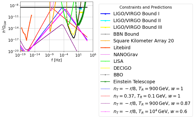
Figure 1: The $h^{2}$-scaled gravitational wave energy spectrum for the $a$-attractors inflationary model (similar for the $R^{2}$ model) with $n_{\mathcal{T}}=-r/8$, and for the Einstein-Gauss-Bonnet model with $n_{\mathcal{T}}=0.37$ for a stiff era occurring when the modes with $k=0.9\,$Mpc^-1 enter the Hubble horizon. The blue curve corresponds to $n_{\mathcal{T}}=-r/8$, $r=0.003$, $w=1$ and a reheating temperature $900\,$GeV, the purple curve to $n_{\mathcal{T}}=-r/8$, $r=0.003$, $w=0.87$ and a reheating temperature $900\,$GeV, the magenta curve to $n_{\mathcal{T}}=-r/8$, $r=0.003$, $w=0.6$ and a reheating temperature $10^{4}\,$GeV, while the red curve to $n_{\mathcal{T}}=0.37$, $r=0.003$, $w=1$ and a reheating temperature $0.1\,$GeV.

The gravitational action of such a theory is,

$$\centering S=\int{d^{4}x\sqrt{-g}\left(\frac{R}{2\kappa^{2}}-\frac{1}{2}\partial_{\mu}\phi\partial^{\mu}\phi-V(\phi)-\frac{1}{2}\xi(\phi)\mathcal{G}\right)}\,,\@add@centering$$ (75)

with $\mathcal{G}$ denoting the Gauss-Bonnet invariant which defined explicitly $\mathcal{G}=R^{2}-4R_{\alpha\beta}R^{\alpha\beta}+R_{\alpha\beta\gamma\delta}R^{\alpha\beta\gamma\delta}$ with $R_{\alpha\beta}$ and $R_{\alpha\beta\gamma\delta}$ denoting as usual the Ricci and Riemann tensors respectively. The speed of the tensor perturbations is demanded to be equal to unity in such theories, thus using this constraint, the slow-roll indices for this theory take the form [146],

$$\centering\epsilon_{1}\simeq\frac{\kappa^{2}}{2}\left(\frac{\xi^{\prime}}{\xi^{\prime\prime}}\right)^{2}\,,\@add@centering$$ (76)

$$\centering\epsilon_{2}\simeq 1-\epsilon_{1}-\frac{\xi^{\prime}\xi^{\prime\prime\prime}}{\xi^{\prime\prime 2}}\,,\@add@centering$$ (77)

$$\centering\epsilon_{3}=0\,,\@add@centering$$ (78)

$$\centering\epsilon_{4}\simeq\frac{\xi^{\prime}}{2\xi^{\prime\prime}}\frac{\mathcal{E}^{\prime}}{\mathcal{E}}\,,\@add@centering$$ (79)

$$\centering\epsilon_{5}\simeq-\frac{\epsilon_{1}}{\lambda}\,,\@add@centering$$ (80)

$$\centering\epsilon_{6}\simeq\epsilon_{5}(1-\epsilon_{1})\,,\@add@centering$$ (81)

where $\mathcal{E}=\mathcal{E}(\phi)$ and also $\lambda=\lambda(\phi)$ are,

$$\mathcal{E}(\phi)=\frac{1}{\kappa^{2}}\left(1+72\frac{\epsilon_{1}^{2}}{\lambda^{2}}\right),\,\,\,\lambda(\phi)=\frac{3}{4\xi^{\prime\prime}\kappa^{2}V}\,.$$ (82)

Accordingly, the observational indices of inflation can be obtained, which are,

$$\centering n_{\mathcal{S}}=1-4\epsilon_{1}-2\epsilon_{2}-2\epsilon_{4}\,,\@add@centering$$ (83)

$$n_{\mathcal{T}}=-2\left(\epsilon_{1}+\epsilon_{6}\right)\,,$$ (84)

$$r=16\left|\left(\frac{\kappa^{2}Q_{e}}{4H}-\epsilon_{1}\right)\frac{2c_{A}^{3}}{2+\kappa^{2}Q_{b}}\right|\,,$$ (85)

and $c_{A}$ denotes the sound speed of the scalar perturbations, which is not trivial and has the following form,

$$\centering c_{A}^{2}=1+\frac{Q_{a}Q_{e}}{3Q_{a}^{2}+\dot{\phi}^{2}(\frac{2}{\kappa^{2}}+Q_{b})}\,,\@add@centering$$ (86)

with,

$$Q_{a}=-4\dot{\xi}H^{2},\,\,\,Q_{b}=-8\dot{\xi}H,\,\,\,Q_{t}=F+\frac{Q_{b}}{2},$$ (87)

$$Q_{c}=0,\,\,\,Q_{e}=-16\dot{\xi}\dot{H}\,.$$

In effect, the tensor-to-scalar ratio and the tensor spectral index take the following form,

$$r\simeq 16\epsilon_{1}\,,$$ (88)

$$n_{\mathcal{T}}\simeq-2\epsilon_{1}\left(1-\frac{1}{\lambda}+\frac{\epsilon_{1}}{\lambda}\right)\,.$$ (89)

We shall use a successful viable model that fits our constraints and the purposes of this analysis, which has the following Gauss-Bonnet coupling function,

$$\xi(\phi)=\beta\exp\left(\left(\frac{\phi}{M}\right)^{2}\right)\,,$$ (90)

with $\beta$ being a dimensionless parameter and $M$ has mass dimensions $[m]^{1}$. The novel feature of the formalism of Ref. [146] is that in order for the theory to be compatible with the GW170817 event, the scalar field potential and the Gauss-Bonnet scalar coupling are not arbitrarily chosen, but are constrained to satisfy a non-trivial differential equation, thus by using the form of the Gauss-Bonnet scalar coupling given in Eq. (90), the scalar potential is found to have this form,

$$\centering V(\phi)=\frac{3}{3\gamma\kappa^{4}+4\beta\kappa^{4}e^{\frac{\phi^{2}}{M^{2}}}}\,,\@add@centering$$ (91)

with $\gamma$ being an integration constant which is dimensionless. Thus using the above formalism, the slow-roll indices in terms of the scalar field easily follow,

$$\centering\epsilon_{1}\simeq\frac{\kappa^{2}M^{4}\phi^{2}}{2\left(M^{2}+2\phi^{2}\right)^{2}}\,,\@add@centering$$ (92)

$$\centering\epsilon_{2}\simeq\frac{M^{4}\left(2-\kappa^{2}\phi^{2}\right)-4M^{2}\phi^{2}}{2\left(M^{2}+2\phi^{2}\right)^{2}}\,,\@add@centering$$ (93)

$$\centering\epsilon_{3}=0\,,\@add@centering$$ (94)

$$\centering\epsilon_{5}\simeq-\frac{4\beta\phi^{2}e^{\frac{\phi^{2}}{M^{2}}}}{\left(M^{2}+2\phi^{2}\right)\left(3\gamma+4\beta e^{\frac{\phi^{2}}{M^{2}}}\right)}\,,\@add@centering$$ (95)

$$\centering\epsilon_{6}\simeq-\frac{2\beta\phi^{2}e^{\frac{\phi^{2}}{M^{2}}}\left(M^{4}\left(2-\kappa^{2}\phi^{2}\right)+8M^{2}\phi^{2}+8\phi^{4}\right)}{\left(M^{2}+2\phi^{2}\right)^{3}\left(3\gamma+4\beta e^{\frac{\phi^{2}}{M^{2}}}\right)}\,,\@add@centering$$ (96)

and accordingly, the scalar spectral index, the tensor spectral index and the tensor-to-scalar ratio are,

$$n_{\mathcal{S}}\simeq-1-\frac{\kappa^{2}M^{4}\phi^{2}}{\left(M^{2}+2\phi^{2}\right)^{2}}+\frac{4\phi^{2}\left(3M^{2}+2\phi^{2}\right)}{\left(M^{2}+2\phi^{2}\right)^{2}}$$ (97)

$$+\frac{4608\beta^{2}\phi^{6}e^{\frac{2\phi^{2}}{M^{2}}}\left(6\gamma\phi^{2}+16\beta e^{\frac{\phi^{2}}{M^{2}}}\left(M^{2}+\phi^{2}\right)+9\gamma M^{2}\right)}{\left(M^{2}+2\phi^{2}\right)^{4}\left(3\gamma+4\beta e^{\frac{\phi^{2}}{M^{2}}}\right)^{3}}\,,$$

regarding the spectral index of scalar perturbations, while spectral index of tensor perturbations reads,

$$n_{\mathcal{T}}\simeq\frac{\phi^{2}\left(-4\beta e^{\frac{\phi^{2}}{M^{2}}}\left(M^{4}\left(3\kappa^{2}\phi^{2}-2\right)+\kappa^{2}M^{6}-8M^{2}\phi^{2}-8\phi^{4}\right)-3\gamma\kappa^{2}M^{4}\left(M^{2}+2\phi^{2}\right)\right)}{\left(M^{2}+2\phi^{2}\right)^{3}\left(3\gamma+4\beta e^{\frac{\phi^{2}}{M^{2}}}\right)}\,,$$ (98)

$$r\simeq\frac{8\kappa^{2}M^{4}\phi^{2}}{\left(M^{2}+2\phi^{2}\right)^{2}}\,.$$ (99)

For our analysis we shall need mildly blue tensor spectral index, so the theory at hand yields such mild values in the range $n_{\mathcal{T}}=[0.378,0.379]$ with a tensor-to-scalar ratio $r\sim 0.003$ when we choose the free variables as follows, $\mu=[22.0914,22.09147]$, $\beta=-1.5$, $\gamma=2$, for approximately $N=60$ $e$-foldings.

After describing the theoretical framework we shall need for our analysis of the energy spectrum of the primordial gravitational waves, let us proceed to the analysis of the energy spectrum of the primordial gravitational waves and the predictions of our approach. We shall examine thoroughly both the theoretical frameworks with blue-tilted and the red-tilted tensor spectrum we analyzed previously. In Fig. 1 we plot the $h^{2}$-scaled gravitational wave energy spectrum for the $a$-attractors inflationary model with $n_{\mathcal{T}}=-r/8$, and for the Einstein-Gauss-Bonnet model with $n_{\mathcal{T}}=0.37$ for a stiff era occurring when the modes with $k=0.9\,$Mpc^-1 enter the Hubble horizon. The blue curve corresponds to $n_{\mathcal{T}}=-r/8$, $r=0.003$, $w=1$, $T_{R}=900\,$GeV and a reheating temperature $900\,$GeV, the purple curve to $n_{\mathcal{T}}=-r/8$, $r=0.003$, $w=0.87$, $T_{R}=900\,$GeV and a reheating temperature $900\,$GeV, the magenta curve to $n_{\mathcal{T}}=-r/8$, $r=0.003$, $w=0.6$, $T_{R}=10^{4}\,$GeV and a reheating temperature $10^{4}\,$GeV, while the red curve to $n_{\mathcal{T}}=0.37$, $r=0.003$, $w=1$, $T_{R}=0.1\,$GeV and a reheating temperature $0.1\,$GeV. Similar results are obtained for the $R^{2}$ model which we omit for brevity. As it can be seen in Fig. 1 the NANOGrav 2023 signal can be explained by the blue-tilted Einstein-Gauss-Bonnet theory we developed previously, with a relatively mild blue-tilted tensor spectral index $n_{\mathcal{T}}=0.37$, and with a stiff era occurring before the CMB and for a reheating temperature of the order $T_{R}=0.1\,$GeV. Thus if the stiff era occurred before the CMB, the modes entering the horizon during that era can significantly affect today’s energy spectrum of the primordial gravitational waves and the predicted signal can explain the NANOGrav 2023 signal. In, addition, the same signal can be detected by the SKA, LISA, the future BBO and DECIGO experiments, but not from the Einstein Telescope. On the other hand, if the inflationary theory is not a blue-tilted one and it is described by the $a$-attractors for example, and a stiff era again occurs before the CMB, the NANOGrav signal cannot be explained by a stiff era, and it can remain undetectable by all the experiments for $w=0.87$, $T_{R}=900\,$GeV, but for $w=0.6$, $T_{R}=10^{4}\,$GeV and $w=1$, $T_{R}=900\,$GeV it can be detected by SKA, LISA, BBO and the DECIGO experiments but not from the Einstein telescope. It is obvious that the synergy between gravitational waves experiments is vital towards understanding the underlying theory that governs the primordial gravitational waves physics. For example the non-detection by the Einstein Telescope may favor the scenarios we develop in this paper and other similar ones. In conclusion, a stiff era before the CMB can enhance the energy spectrum of the gravitational waves significantly. How about having several deformations of the background EoS from reheating up to the CMB scales. Imagine that several deformations may occur and so the modes entering the horizon at different eras, may affect the energy spectrum. We shall discuss such scenario in the following section.

III Higgs-Axion Higher Order Couplings and Multiple Post-Electroweak Breaking Axion Stiff Eras

So far we did not consider a specific model that may yield stiff deformations of the total EoS of the Universe slightly before the recombination era, since we used an agnostic approach for this procedure. Now we shall propose a model that may explain such a total EoS deformation. This model is based on a Higgs-axion model with higher order non-renormalizable couplings, which after the electroweak breaking occurs, affect drastically the axion potential as we explain shortly. This model is based on the fact that the electroweak breaking actually occurs at some point in the past. In all the cases in the literature, the electroweak symmetry breaking occurs in terms of a thermal first order phase transition with the symmetry breaking transition being of the order $T\sim 100\,$GeV [163, 164, 165, 166, 167, 168, 169, 170, 171, 172, 173, 166, 174, 175, 176, 177, 178, 179, 167, 180, 181, 182, 183]. As we saw in the previous section, in order for the NANOGrav signal to be explained by an inflationary theory in conjunction with a stiff deformation of the total EoS parameter before the recombination era, a low reheating temperature is required, of the order $T\sim 0.1\,$GeV. Now, this feature can put the electroweak symmetry breaking phase transition in peril of existence if it occurs thermally. However there exist other ways to break the electroweak symmetry, that do not invoke a thermal phase transition. We are developing such a theory currently the details of which will be given elsewhere [184]. For the moment we shall assume that a high reheating temperature is not required for breaking the electroweak symmetry and that this breaks non-thermally at some point during the inflationary era.

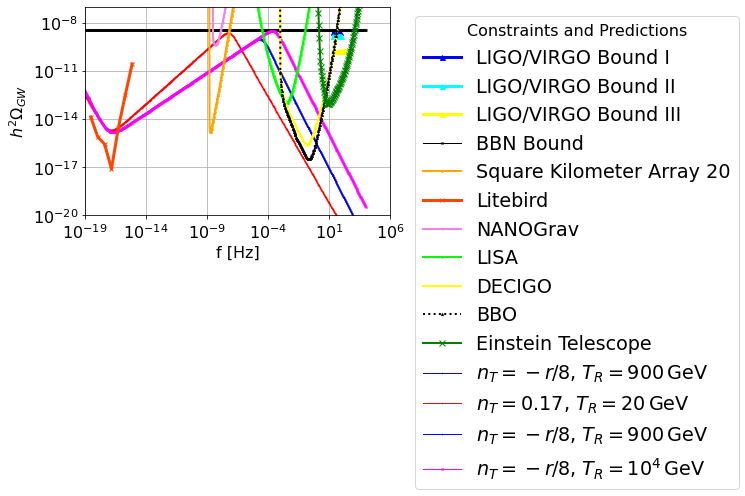
Figure 2: The $h^{2}$-scaled gravitational wave energy spectrum for the $a$-attractors inflationary model (similar for the $R^{2}$ model) with $n_{\mathcal{T}}=-r/8$, and for the Einstein-Gauss-Bonnet model with $n_{\mathcal{T}}=0.17$ for several deformations of the total background EoS caused by the axion movements towards the new minimum of its potential at the post-electroweak symmetry breaking epoch. These deformations in this scenario occur and affect the modes with wavenumbers $k_{w_{1}}=0.001$Mpc^-1, $k_{w_{2}}=0.004$Mpc^-1, $k_{w_{3}}=0.9$Mpc^-1, $k_{t_{1}}=15\times 10^{5}$Mpc^-1 , $k_{t_{2}}=10\times 10^{9}$Mpc^-1, $k_{t_{3}}=10\times 10^{10}$Mpc^-1. For those distinct epochs we shall assume that the total background EoS parameter has the values $w_{c}=0.34$ for $k_{w_{1}}$, $k_{w_{2}}$ and $k_{t_{2}}$, $w_{c_{1}}=1$ for the modes $k_{w_{3}}$, $w_{b}=0.25$ for the modes $k_{t_{1}}$ and $k_{t_{3}}$. The blue curve corresponds to $n_{\mathcal{T}}=-r/8$, $r=0.003$, and a reheating temperature $900\,$GeV, the magenta curve to $n_{\mathcal{T}}=-r/8$, $r=0.003$, and a reheating temperature $10^{4}\,$GeV, while the red curve to $n_{\mathcal{T}}=0.17$, $r=0.003$, and a reheating temperature $20\,$GeV.

Now let us discuss in detail the physics of the Higgs-Axion model that may explain the deformations of the total EoS of the Universe after the electroweak symmetry breaking and of course before the CMB era and even after the recombination era, up to present day. This model was developed in detail in Ref. [95] and we shall briefly discuss the essential features of this model. It is based on non-renormalizable higher order operators that couple non-trivial and holomorphically the Higgs and the axion, and for general Higgs-axion couplings in other contexts, mainly renormalizable, see for example [185, 186, 187]. The latter is one of the main dark matter candidates at present day [188, 189, 190, 191, 192, 193, 194, 195, 196, 197, 198, 208, 200, 201, 202, 203, 204, 205, 72, 206, 207, 208, 209, 210, 211]. Assuming the misalignment axion scenario, which is based on the pre-inflationary breaking of the axion Peccei-Quinn $U(1)$. During inflation, and before the electroweak symmetry breaking, the axion is misaligned from the minimum of its potential, which can be approximated by,

$$V_{a}(\phi)\simeq\frac{1}{2}m_{a}^{2}\phi^{2}\,.$$ (100)

When the Hubble rate becomes of the order of the axion mass, the axion commences oscillations and thus redshifts as dark matter. We modify the axion sector by adding the following higher order non-renormalizable operators of the axion to the Higgs,

$$V(\phi,h)=V_{a}(\phi)-m_{H}^{2}|H|^{2}+\lambda_{H}|H|^{4}-\lambda\frac{|H|^{2}\phi^{4}}{M^{2}}+g\frac{|H|^{2}\phi^{6}}{M^{4}}\,,$$ (101)

with $V_{a}(\phi)$ being defined in Eq. (100), and note that the Higgs field at the pre-electroweak symmetry breaking era is $H=\frac{h+ih_{1}}{\sqrt{2}}$, with $m_{H}=125$ GeV [212] and $\lambda_{H}$ is defined via $\frac{v}{\sqrt{2}}=\left(\frac{-m_{H}^{2}}{\lambda_{H}}\right)^{\frac{1}{2}}$, and finally $v$ is the electroweak symmetry breaking scale which is approximately $v\simeq 246\,$GeV. We also take the axion mass to be $m_{a}\sim 10^{-10}\,$eV and the effective theory scale $M$ to be $M=20-100\,$TeV. Also the Wilson coefficients are taken to be $\lambda\sim\mathcal{O}(10^{-20})$ and $g\sim\mathcal{O}(10^{-5})$. When the electroweak breaking occurs, the Higgs field becomes $H=v+\frac{h+ih_{1}}{\sqrt{2}}$, and hence at leading order, the axion potential at one-loop zero temperature takes the form,

$$\mathcal{V}_{a}(\phi)=V_{a}(\phi)-\lambda\frac{v^{2}\phi^{4}}{M^{2}}+g\frac{v^{2}\phi^{6}}{M^{6}}+\frac{m_{eff}^{4}(\phi)}{64\pi^{2}}\left(\ln\left(\frac{m_{eff}^{2}(\phi)}{\mu^{2}}\right)-\frac{3}{2}\right)\,,$$ (102)

where $m_{eff}^{2}(\phi)$,

$$m_{eff}^{2}(\phi)=\frac{\partial^{2}V(\phi,h)}{\partial\phi^{2}}=m_{a}^{2}-\frac{6\lambda v^{2}\phi^{2}}{M^{2}}+\frac{15gv^{2}\phi^{4}}{M^{4}}\,,$$ (103)

and also $\mu$ denotes the renormalization scale. In this model, after the electroweak symmetry breaking, the axion potential develops a minimum which is lower from the original minimum. Hence the axion begins rolling towards the new minimum, which can be done in a rapid or a slow-roll way. Hence, the dark matter nature of the axion is disrupted at some point, and when the axion is destabilized, the axion rolls towards the new minimum, in a stiff way as we shall assume in this paper. Once the minimum is reached, since the Higgs minimum $(h,\phi)=(v,0)$ is energetically favorable compared to the axion minimum $(h,\phi)=(0,v_{s})$, that is,

$$V_{h}(h)=(v)\gg V(\phi)=(v_{s})\,,$$ (104)

therefore, the axion vacuum decays to the Higgs vacuum and the axion starts again in the origin its oscillations, behaving as dark matter again. The procedure repeats itself perpetually and thus we have interchanging eras of dark matter and stiff axion EoS. Now depending on the total background EoS parameter, the energy spectrum may be affected significantly. At this point we shall examine some scenarios and their effect on the energy spectrum of the primordial gravitational waves. Let us consider a sequence of deformations of the background EoS due to the axion moving in a kinetic way to the new minimum of its potential in the post-electroweak era. Let us suppose that these deformations of the EoS occurred at several distinct epochs starting from reheating and up to modes that reentered the Hubble horizon just before the CMB but also after the CMB occurred. So consider that the background EoS occurred at epochs in which the modes with wavenumbers $k_{w_{1}}=0.001$Mpc^-1, $k_{w_{2}}=0.004$Mpc^-1, $k_{w_{3}}=0.9$Mpc^-1, $k_{t_{1}}=15\times 10^{5}$Mpc^-1 , $k_{t_{2}}=10\times 10^{9}$Mpc^-1, $k_{t_{3}}=10\times 10^{10}$Mpc^-1. For those distinct epochs we shall assume that the total background EoS parameter has the values $w_{c}=0.34$ for $k_{w_{1}}$, $k_{w_{2}}$ and $k_{t_{2}}$, $w_{c_{1}}=1$ for the modes $k_{w_{3}}$, $w_{b}=0.25$ for the modes $k_{t_{1}}$ and $k_{t_{3}}$. The inflationary theory is assumed to be one from the $a$-attractors or the $R^{2}$, which have red tilt or the Einstein-Gauss-Bonnet theory we developed in the previous section, which has a blue-tilted tensor spectral index.

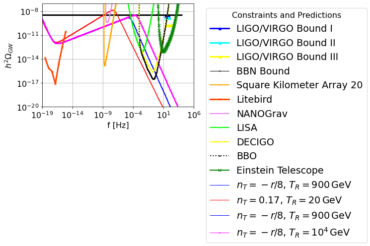
Figure 3: The $h^{2}$-scaled gravitational wave energy spectrum for the $a$-attractors inflationary model (similar for the $R^{2}$ model) with $n_{\mathcal{T}}=-r/8$, and for the Einstein-Gauss-Bonnet model with $n_{\mathcal{T}}=0.17$ for several deformations of the total background EoS caused by the axion movements towards the new minimum of its potential at the post-electroweak symmetry breaking epoch. These deformations in this scenario occur and affect the modes with wavenumbers $k_{w_{1}}=0.001$Mpc^-1, $k_{w_{2}}=0.004$Mpc^-1, $k_{w_{3}}=0.9$Mpc^-1, $k_{t_{1}}=15\times 10^{5}$Mpc^-1 , $k_{t_{2}}=10\times 10^{9}$Mpc^-1, $k_{t_{3}}=10\times 10^{10}$Mpc^-1. For those distinct epochs we shall assume that the total background EoS parameter has the values $w_{c}=0.34$ for $k_{w_{1}}$, $k_{w_{2}}$ and $k_{t_{2}}$, $w_{c_{1}}=1$ for the modes $k_{w_{3}}$, $w_{b}=0.25$ for the mode $k_{t_{1}}$, and $w=0.2$ for the mode $k_{t_{3}}$. The blue curve corresponds to $n_{\mathcal{T}}=-r/8$, $r=0.003$, and a reheating temperature $900\,$GeV, the magenta curve to $n_{\mathcal{T}}=-r/8$, $r=0.003$, and a reheating temperature $10^{4}\,$GeV, while the red curve to $n_{\mathcal{T}}=0.17$, $r=0.003$, and a reheating temperature $20\,$GeV.

For the deformations of the total background EoS parameter, the energy spectrum is instantaneously modified as follows,

$$\Omega_{\rm gw}(f)=S_{k}(f)\times\frac{k^{2}}{12H_{0}^{2}}r\mathcal{P}_{\zeta}(k_{ref})\left(\frac{k}{k_{ref}}\right)^{n_{\mathcal{T}}}\left(\frac{\Omega_{m}}{\Omega_{\Lambda}}\right)^{2}\left(\frac{g_{*}(T_{\rm in})}{g_{*0}}\right)\left(\frac{g_{*s0}}{g_{*s}(T_{\rm in})}\right)^{4/3}\left(\overline{\frac{3j_{1}(k\tau_{0})}{k\tau_{0}}}\right)^{2}T_{1}^{2}\left(x_{\rm eq}\right)T_{2}^{2}\left(x_{R}\right)\,,$$

with the multiplication factor $S_{k}(f)$ being,

$$S_{k}(f)=\left(\frac{k}{k_{t_{1}}}\right)^{r_{b}}\times\left(\frac{k}{k_{t_{2}}}\right)^{r_{c}}\times\left(\frac{k}{k_{t_{3}}}\right)^{r_{b}}\times\left(\frac{k}{k_{w_{1}}}\right)^{r_{c}}\times\left(\frac{k}{k_{w_{2}}}\right)^{r_{c}}\times\left(\frac{k}{k_{w_{3}}}\right)^{r_{c_{1}}}\,,$$ (105)

with $r_{b}=-2\left(\frac{1-3w_{b}}{1+3w_{b}}\right)$, $r_{c}=-2\left(\frac{1-3w_{c}}{1+3w_{c}}\right)$ and $r_{c_{1}}=-2\left(\frac{1-3w_{c_{1}}}{1+3w_{c_{1}}}\right)$ and recall that $w_{c}=0.34$ for $k_{w_{1}}$, $k_{w_{2}}$ and $k_{t_{2}}$, $w_{c_{1}}=1$ for the modes $k_{w_{3}}$, $w_{b}=0.25$ for the modes $k_{t_{1}}$ and $k_{t_{3}}$. [93]. In Fig. 2 we present the predicted the energy spectrum of the primordial gravitational waves for the model at hand for various reheating temperatures and for the red-tilted tensor and for the blue-tilted tensor spectral index. The blue curve corresponds to $n_{\mathcal{T}}=-r/8$, $r=0.003$, and a reheating temperature $900\,$GeV, the magenta curve to $n_{\mathcal{T}}=-r/8$, $r=0.003$, and a reheating temperature $10^{4}\,$GeV, while the red curve to $n_{\mathcal{T}}=0.17$, $r=0.003$, and a reheating temperature $20\,$GeV. Thus for the blue-tilted tensor case we used even milder values for the blue tilt of the tensor spectral index and higher for the reheating temperature. As it can be seen, the NANOGrav signal is explained by the Einstein-Gauss-Bonnet theory with a milder blue tilt in the tensor spectral index, compared to the values used in the previous section, and a low reheating temperature, and also the same signal can be detected by LISA, DECIGO and the BBO detectors, but not from the Einstein Telescope. Regarding the red-tilted theory, it predicts an energy spectrum that can be detected by LISA, DECIGO and the BBO detector but not from the Einstein Telescope. Now the striking new feature is that in all these cases, the Litebird experiment may detect the predicted signals. In fact the signal might become stronger if the era in which the modes with $k_{t_{3}}=10\times 10^{10}$Mpc^-1 reentered the Hubble horizon, had a background EoS parameter $w=0.2$, thus closer to the matter dominated epoch. This can be seen in Fig. 3. The red curve is incompatible with the Big Bang Nucleosynthesis constraints, but we just wanted to make a point here, that the signal can be more pronounced if the modes with $k_{t_{3}}=10\times 10^{10}$Mpc^-1 reentered the Hubble horizon, had a background EoS parameter $w<0.25$.

Thus the striking new feature of this model is the prediction that Litebird might detect the tail of this signal, indicating to an era with background EoS parameter of the order $w=0.2$ for modes with wavenumber $k\sim\mathcal{O}(10^{10})$Mpc^-1 which reentered the horizon during that epoch. Finally, let us mention again that in order for this model to explain the NANOGrav 2023 signal a low-reheating temperature is required. Now recall that this model is based on the fact that the electroweak phase transition takes place primordially, thus with such a low-reheating temperature, it is impossible to break the electroweak symmetry thermally. However there exist other ways to break the electroweak symmetry, apart from the thermal phase transition. We are developing such a model and will report on this soon [184].

III.1 Brief Comment on the Effects of a Short Stiff pre-CMB Era on the BBN and CMB

Let us here discuss a somewhat important issue regarding the BBN and CMB effects of a short stiff era that occurred just before the CMB era and well beyond the matter-radiation equality. As we will show, since we considered modes with $k=0.9\,$Mpc^-1, neither the CMB or the BBN is affected by the short stiff era.

Let us discuss first the BBN issues, which has also been addressed in [92]. An even short stiff era could affect the abundance of light elements, in two ways. If the stiff era occurred before the BBN, so when the temperature was $T>0.1\,$MeV, this would affect the helium abundance which is quite sensitive to the freeze out of proton-neutron conversions. Thus since in our case the stiff era occurs before the CMB, the abundance of helium is not affected at all. After the BBN a stiff era would only affect the abundance of deuterium, which eventually freezes at the last stages of the BBN. Following [92], the constraint that must be satisfied in order not to affect the deuterium abundance is that the temperature at which the kination era commences must be $T_{K}<6\,$keV. In our case the stiff era occurs just before the CMB and well after the matter-radiation equality, thus the temperature is of the order $\sim 0.5\,$eV or slightly smaller or even slightly larger. Thus, as it proves there is no issue related to the abundances of light elements.

Let us discuss the issues that may come up with the CMB. However even the question of affecting the CMB modes with a stiff era that occurs when modes of the order $k=0.9\,$Mpc^-1 (see Fig. 1) is rather futile. The reason is that modes with $\lambda<10\,$Mpc or equivalently modes with wavenumber $k>0.628319\,$Mpc^-1 cannot be analyzed using linear perturbation theory. Thus since we chose to study modes with $k=0.9\,$Mpc^-1, the linear perturbation theory theory cannot be used and therefore no primary effects are expected in the CMB polarization, only secondary non-linear effects. And also it might be possible that these effects might affect the energy spectrum of primordial gravitational waves by providing an enhancement of the spectrum. This analysis though exceeds the aims and scopes of this article, which were to demonstrate the direct effects of a pre-CMB era on the energy spectrum of the primordial gravitational waves.

But for completeness, and since at a later section we used modes with $k<0.628319\,$Mpc^-1 but we did not take these into account in the figures, let us qualitatively discuss the effects of a pre-CMB era on the CMB. The kination era could directly affect the sound horizon at the last scattering surface and actually the angular scale of the sound horizon. This is not an easy problem to address and solve though, since there are quite many parameters which if their value changes, can compensate the effects of the stiff era on the sound horizon, for example a changes in $H_{0}$, or the baryon fraction and so on. Also the duration of the stiff era plays a role, which was not considered [92] but was analyzed in [93]. Hence, the problem is not so easy to solve, and in order to fully address it the coupled Boltzmann equations which describe the evolution of matter perturbations and gravitational perturbations must be solved, and also allow changes in $H_{0}$, the baryon fraction and other parameters. This analysis stretches by far beyond the scopes of this demonstrative article. Besides, our main assumption was that the stiff era occurred when modes with wavenumber $k=0.9\,$Mpc^-1 reentered the Hubble horizon, thus these modes cannot be treated by using linear perturbation theory. Hence the whole argument against a stiff era does not apply in our case.

Concluding Remarks and Discussion

In this work we thoroughly examined the quantitative effects of a stiff era occurring before the CMB era, on the energy spectrum of the primordial gravitational waves at present day. Firstly, in a model-agnostic way without giving any reasoning for this kination era, we examined the effect of this era on the modes that reentered the horizon during this pre-recombination stiff era. For our quantitative analysis we focused on modes having wavenumber $k\sim 0.9\,$Mpc^-1 and also we assumed some inflationary era, focusing on viable models. Specifically, the inflationary era can be realized by a model which generates a red-tilted tensor spectral index, like the $a$-attractors or the $R^{2}$ model, or by a model that can generate a blue-tilted tensor spectral index, like the Einstein-Gauss-Bonnet models. If at the time of the reentry in the Hubble horizon of the modes with wavenumber $k\sim 0.9\,$Mpc^-1, the total background EoS parameter describes a kination era, then the predicted signal can be detected by several current and future gravitational wave experiments. Specifically, if the inflationary era has a mild blue-tilted tensor spectral index of the order $n_{\mathcal{T}}\sim 0.37$ and if the reheating temperature is of the order $T_{R}\sim\mathcal{O}(0.1)$GeV, the signal can explain the 2023 NANOGrav detection of the stochastic gravitational wave background, and also the signal can be detectable by the future SKA experiment. Accordingly, if the reheating temperature is significantly higher and a red-tilted inflationary is assumed, the predicted energy spectrum will be detectable by the future LISA, DECIGO and BBO experiments. After the model-agnostic approach, we considered a specific model invoking Higgs-axion higher order non-renormalizable couplings. This model is based on the occurrence of the electroweak symmetry breaking, which however cannot occur thermally if the reheating temperature never reached at least 100GeV. There are ways to break the electroweak symmetry apart from thermal phase transitions [184], thus for the analysis of this section we assumed that the electroweak symmetry breaking occurred in a non-thermal way. Having settled that, we analyzed the Higgs-axion model which predicts that multiple stiff eras may occur after the electroweak symmetry breaking, specifically, during reheating, matter domination era, before and after recombination. These axion stiff eras changes the background EoS parameter at these eras, thus affect the modes that reenter the Hubble horizon during these eras. As we demonstrated, the 2023 NANOGrav stochastic gravitational wave signal can be explained by this model, if the reheating temperature is of the order $T_{R}\sim 20$GeV and the inflationary era has a really mild blue-tilted tensor spectral index $n_{\mathcal{T}}\sim 0.17$. The same signal can be detectable by the SKA. Also for a red-tilted tensor spectral index, the energy spectrum can be detected by LISA, BBO and DECIGO. More importantly, in all cases, this model generates a stochastic signal that can be detected by Litebird, which is a characteristic feature of this model. In all cases, for both the model-agnostic approach and for the specific model which we analyzed, the signal cannot be detectable by the Einstein Telescope. This brings us to the important line of thinking, that only the synergy of current and future gravitational wave experiments can yield decisive information regarding the actual source of the stochastic gravitational wave background. Patterns like the ones we described in this paper, will be indicative for the underlying theory that governs the stochastic gravitational wave background. For example in the Higgs-axion model, the blue-tilted tensor spectral index model can be detected from the future Litebird and the current NANOGrav experiment, and from no other gravitational wave experiment. This is a characteristic pattern. Thus the way towards understanding the primordial Universe will be based on the synergy between current and future gravitational wave experiments. Exciting upcoming years for science to say the least.

References

- [1] A. D. Linde, Lect. Notes Phys. 738 (2008) 1 [arXiv:0705.0164 [hep-th]].
- [2] D. S. Gorbunov and V. A. Rubakov, “Introduction to the theory of the early universe: Cosmological perturbations and inflationary theory,” Hackensack, USA: World Scientific (2011) 489 p;
- [3] A. Linde, arXiv:1402.0526 [hep-th];
- [4] D. H. Lyth and A. Riotto, Phys. Rept. 314 (1999) 1 [hep-ph/9807278].
- [5] K. N. Abazajian et al. [CMB-S4], [arXiv:1610.02743 [astro-ph.CO]].
- [6] M. H. Abitbol et al. [Simons Observatory], Bull. Am. Astron. Soc. 51 (2019), 147 [arXiv:1907.08284 [astro-ph.IM]].
- [7] S. Hild, M. Abernathy, F. Acernese, P. Amaro-Seoane, N. Andersson, K. Arun, F. Barone, B. Barr, M. Barsuglia and M. Beker, et al. Class. Quant. Grav. 28 (2011), 094013 doi:10.1088/0264-9381/28/9/094013 [arXiv:1012.0908 [gr-qc]].
- [8] J. Baker, J. Bellovary, P. L. Bender, E. Berti, R. Caldwell, J. Camp, J. W. Conklin, N. Cornish, C. Cutler and R. DeRosa, et al. [arXiv:1907.06482 [astro-ph.IM]].
- [9] T. L. Smith and R. Caldwell, Phys. Rev. D 100 (2019) no.10, 104055 doi:10.1103/PhysRevD.100.104055 [arXiv:1908.00546 [astro-ph.CO]].
- [10] J. Crowder and N. J. Cornish, Phys. Rev. D 72 (2005), 083005 doi:10.1103/PhysRevD.72.083005 [arXiv:gr-qc/0506015 [gr-qc]].
- [11] T. L. Smith and R. Caldwell, Phys. Rev. D 95 (2017) no.4, 044036 doi:10.1103/PhysRevD.95.044036 [arXiv:1609.05901 [gr-qc]].
- [12] N. Seto, S. Kawamura and T. Nakamura, Phys. Rev. Lett. 87 (2001), 221103 doi:10.1103/PhysRevLett.87.221103 [arXiv:astro-ph/0108011 [astro-ph]].
- [13] S. Kawamura, M. Ando, N. Seto, S. Sato, M. Musha, I. Kawano, J. Yokoyama, T. Tanaka, K. Ioka and T. Akutsu, et al. [arXiv:2006.13545 [gr-qc]].
- [14] A. Weltman, P. Bull, S. Camera, K. Kelley, H. Padmanabhan, J. Pritchard, A. Raccanelli, S. Riemer-Sørensen, L. Shao and S. Andrianomena, et al. Publ. Astron. Soc. Austral. 37 (2020), e002 doi:10.1017/pasa.2019.42 [arXiv:1810.02680 [astro-ph.CO]].
- [15] P. Auclair et al. [LISA Cosmology Working Group], [arXiv:2204.05434 [astro-ph.CO]].
- [16] G. Agazie et al. [NANOGrav], doi:10.3847/2041-8213/acdac6 [arXiv:2306.16213 [astro-ph.HE]].
- [17] J. Antoniadis, P. Arumugam, S. Arumugam, S. Babak, M. Bagchi, A. S. B. Nielsen, C. G. Bassa, A. Bathula, A. Berthereau and M. Bonetti, et al. [arXiv:2306.16214 [astro-ph.HE]].
- [18] D. J. Reardon, A. Zic, R. M. Shannon, G. B. Hobbs, M. Bailes, V. Di Marco, A. Kapur, A. F. Rogers, E. Thrane and J. Askew, et al. doi:10.3847/2041-8213/acdd02 [arXiv:2306.16215 [astro-ph.HE]].
- [19] H. Xu, S. Chen, Y. Guo, J. Jiang, B. Wang, J. Xu, Z. Xue, R. N. Caballero, J. Yuan and Y. Xu, et al. doi:10.1088/1674-4527/acdfa5 [arXiv:2306.16216 [astro-ph.HE]].
- [20] S. Vagnozzi, JHEAp 39 (2023), 81-98 doi:10.1016/j.jheap.2023.07.001 [arXiv:2306.16912 [astro-ph.CO]].
- [21] V. K. Oikonomou, Phys. Rev. D 108 (2023) no.4, 043516 doi:10.1103/PhysRevD.108.043516 [arXiv:2306.17351 [astro-ph.CO]].
- [22] Y. F. Cai, X. C. He, X. Ma, S. F. Yan and G. W. Yuan, [arXiv:2306.17822 [gr-qc]].
- [23] C. Han, K. P. Xie, J. M. Yang and M. Zhang, [arXiv:2306.16966 [hep-ph]].
- [24] S. Y. Guo, M. Khlopov, X. Liu, L. Wu, Y. Wu and B. Zhu, [arXiv:2306.17022 [hep-ph]].
- [25] J. Yang, N. Xie and F. P. Huang, [arXiv:2306.17113 [hep-ph]].
- [26] A. Addazi, Y. F. Cai, A. Marciano and L. Visinelli, [arXiv:2306.17205 [astro-ph.CO]].
- [27] S. P. Li and K. P. Xie, Phys. Rev. D 108 (2023) no.5, 055018 doi:10.1103/PhysRevD.108.055018 [arXiv:2307.01086 [hep-ph]].
- [28] X. Niu and M. H. Rahat, [arXiv:2307.01192 [hep-ph]].
- [29] A. Yang, J. Ma, S. Jiang and F. P. Huang, [arXiv:2306.17827 [hep-ph]].
- [30] S. Datta, [arXiv:2307.00646 [hep-ph]].
- [31] X. K. Du, M. X. Huang, F. Wang and Y. K. Zhang, [arXiv:2307.02938 [hep-ph]].
- [32] A. Salvio, [arXiv:2307.04694 [hep-ph]].
- [33] Z. Yi, Q. Gao, Y. Gong, Y. Wang and F. Zhang, [arXiv:2307.02467 [gr-qc]].
- [34] Z. Q. You, Z. Yi and Y. Wu, [arXiv:2307.04419 [gr-qc]].
- [35] S. Wang and Z. C. Zhao, [arXiv:2307.04680 [astro-ph.HE]].
- [36] D. G. Figueroa, M. Pieroni, A. Ricciardone and P. Simakachorn, [arXiv:2307.02399 [astro-ph.CO]].
- [37] S. Choudhury, [arXiv:2307.03249 [astro-ph.CO]].
- [38] S. A. Hosseini Mansoori, F. Felegray, A. Talebian and M. Sami, [arXiv:2307.06757 [astro-ph.CO]].
- [39] S. Ge, [arXiv:2307.08185 [gr-qc]].
- [40] L. Bian, S. Ge, J. Shu, B. Wang, X. Y. Yang and J. Zong, [arXiv:2307.02376 [astro-ph.HE]].
- [41] M. Kawasaki and K. Murai, [arXiv:2308.13134 [astro-ph.CO]].
- [42] Z. Yi, Z. Q. You and Y. Wu, [arXiv:2308.05632 [astro-ph.CO]].
- [43] H. An, B. Su, H. Tai, L. T. Wang and C. Yang, [arXiv:2308.00070 [astro-ph.CO]].
- [44] Z. Zhang, C. Cai, Y. H. Su, S. Wang, Z. H. Yu and H. H. Zhang, [arXiv:2307.11495 [hep-ph]].
- [45] P. Di Bari and M. H. Rahat, [arXiv:2307.03184 [hep-ph]].
- [46] S. Jiang, A. Yang, J. Ma and F. P. Huang, [arXiv:2306.17827 [hep-ph]].
- [47] G. Bhattacharya, S. Choudhury, K. Dey, S. Ghosh, A. Karde and N. S. Mishra, [arXiv:2309.00973 [astro-ph.CO]].
- [48] S. Choudhury, A. Karde, S. Panda and M. Sami, [arXiv:2308.09273 [astro-ph.CO]].
- [49] T. Bringmann, P. F. Depta, T. Konstandin, K. Schmidt-Hoberg and C. Tasillo, [arXiv:2306.09411 [astro-ph.CO]].
- [50] S. Choudhury, S. Panda and M. Sami, JCAP 08 (2023), 078 doi:10.1088/1475-7516/2023/08/078 [arXiv:2304.04065 [astro-ph.CO]].
- [51] S. Choudhury, A. Karde, S. Panda and M. Sami, [arXiv:2306.12334 [astro-ph.CO]].
- [52] H. L. Huang, Y. Cai, J. Q. Jiang, J. Zhang and Y. S. Piao, [arXiv:2306.17577 [gr-qc]].
- [53] J. Q. Jiang, Y. Cai, G. Ye and Y. S. Piao, [arXiv:2307.15547 [astro-ph.CO]].
- [54] M. Zhu, G. Ye and Y. Cai, [arXiv:2307.16211 [astro-ph.CO]].
- [55] I. Ben-Dayan, U. Kumar, U. Thattarampilly and A. Verma, [arXiv:2307.15123 [astro-ph.CO]].
- [56] G. Franciolini, A. Iovino, Junior., V. Vaskonen and H. Veermae, [arXiv:2306.17149 [astro-ph.CO]].
- [57] J. Ellis, M. Fairbairn, G. Franciolini, G. Hütsi, A. Iovino, M. Lewicki, M. Raidal, J. Urrutia, V. Vaskonen and H. Veermäe, [arXiv:2308.08546 [astro-ph.CO]].
- [58] L. Liu, Z. C. Chen and Q. G. Huang, [arXiv:2307.01102 [astro-ph.CO]].
- [59] L. Liu, Z. C. Chen and Q. G. Huang, [arXiv:2307.14911 [astro-ph.CO]].
- [60] E. Madge, E. Morgante, C. Puchades-Ibáñez, N. Ramberg, W. Ratzinger, S. Schenk and P. Schwaller, [arXiv:2306.14856 [hep-ph]].
- [61] M. X. Huang, F. Wang and Y. K. Zhang, [arXiv:2309.06378 [hep-ph]].
- [62] C. Fu, J. Liu, X. Y. Yang, W. W. Yu and Y. Zhang, [arXiv:2308.15329 [astro-ph.CO]].
- [63] R. Maji and W. I. Park, [arXiv:2308.11439 [hep-ph]].
- [64] M. R. Gangopadhyay, V. V. Godithi, K. Ichiki, R. Inui, T. Kajino, A. Manusankar, G. J. Mathews and Yogesh, [arXiv:2309.03101 [astro-ph.CO]].
- [65] P. Schwaller, Phys. Rev. Lett. 115 (2015) no.18, 181101 doi:10.1103/PhysRevLett.115.181101 [arXiv:1504.07263 [hep-ph]].
- [66] W. Ratzinger and P. Schwaller, SciPost Phys. 10 (2021) no.2, 047 doi:10.21468/SciPostPhys.10.2.047 [arXiv:2009.11875 [astro-ph.CO]].
- [67] A. Ashoorioon, K. Rezazadeh and A. Rostami, Phys. Lett. B 835 (2022), 137542 doi:10.1016/j.physletb.2022.137542 [arXiv:2202.01131 [astro-ph.CO]].
- [68] S. Choudhury, M. R. Gangopadhyay and M. Sami, [arXiv:2301.10000 [astro-ph.CO]].
- [69] S. Choudhury, S. Panda and M. Sami, [arXiv:2302.05655 [astro-ph.CO]].
- [70] S. Choudhury, S. Panda and M. Sami, [arXiv:2303.06066 [astro-ph.CO]].
- [71] L. Bian, S. Ge, C. Li, J. Shu and J. Zong, [arXiv:2212.07871 [hep-ph]].
- [72] C. S. Machado, W. Ratzinger, P. Schwaller and B. A. Stefanek, JHEP 01 (2019), 053 doi:10.1007/JHEP01(2019)053 [arXiv:1811.01950 [hep-ph]].
- [73] T. Regimbau, Symmetry 14 (2022) no.2, 270 doi:10.3390/sym14020270
- [74] L. Sampson, N. J. Cornish and S. T. McWilliams, Phys. Rev. D 91 (2015) no.8, 084055 doi:10.1103/PhysRevD.91.084055 [arXiv:1503.02662 [gr-qc]].
- [75] G. Agazie et al. [NANOGrav], [arXiv:2306.16221 [astro-ph.HE]].
- [76] G. Sato-Polito and M. Kamionkowski, [arXiv:2305.05690 [astro-ph.CO]].
- [77] R. Ding and C. Tian, [arXiv:2309.01643 [astro-ph.CO]].
- [78] M. Benetti, L. L. Graef and S. Vagnozzi, Phys. Rev. D 105 (2022) no.4, 043520 doi:10.1103/PhysRevD.105.043520 [arXiv:2111.04758 [astro-ph.CO]].
- [79] S. Vagnozzi, Mon. Not. Roy. Astron. Soc. 502 (2021) no.1, L11-L15 doi:10.1093/mnrasl/slaa203 [arXiv:2009.13432 [astro-ph.CO]].
- [80] V. Kamali and R. Brandenberger, Phys. Rev. D 101 (2020) no.10, 103512 doi:10.1103/PhysRevD.101.103512 [arXiv:2002.09771 [hep-th]].
- [81] R. H. Brandenberger, Class. Quant. Grav. 32 (2015) no.23, 234002 doi:10.1088/0264-9381/32/23/234002 [arXiv:1505.02381 [hep-th]].
- [82] R. H. Brandenberger, S. Kanno, J. Soda, D. A. Easson, J. Khoury, P. Martineau, A. Nayeri and S. P. Patil, JCAP 11 (2006), 009 doi:10.1088/1475-7516/2006/11/009 [arXiv:hep-th/0608186 [hep-th]].
- [83] A. Ashtekar and P. Singh, Class. Quant. Grav. 28 (2011), 213001 doi:10.1088/0264-9381/28/21/213001 [arXiv:1108.0893 [gr-qc]].
- [84] M. Bojowald, G. Calcagni and S. Tsujikawa, JCAP 11 (2011), 046 doi:10.1088/1475-7516/2011/11/046 [arXiv:1107.1540 [gr-qc]].
- [85] J. Mielczarek, Phys. Rev. D 79 (2009), 123520 doi:10.1103/PhysRevD.79.123520 [arXiv:0902.2490 [gr-qc]].
- [86] M. Bojowald, Class. Quant. Grav. 26 (2009), 075020 doi:10.1088/0264-9381/26/7/075020 [arXiv:0811.4129 [gr-qc]].
- [87] G. Calcagni and S. Kuroyanagi, JCAP 03 (2021), 019 doi:10.1088/1475-7516/2021/03/019 [arXiv:2012.00170 [gr-qc]].
- [88] A. S. Koshelev, K. Sravan Kumar, A. Mazumdar and A. A. Starobinsky, JHEP 06 (2020), 152 doi:10.1007/JHEP06(2020)152 [arXiv:2003.00629 [hep-th]].
- [89] A. S. Koshelev, K. Sravan Kumar and A. A. Starobinsky, JHEP 03 (2018), 071 doi:10.1007/JHEP03(2018)071 [arXiv:1711.08864 [hep-th]].
- [90] M. Baumgart, J. J. Heckman and L. Thomas, JCAP 07 (2022) no.07, 034 doi:10.1088/1475-7516/2022/07/034 [arXiv:2109.08166 [hep-ph]].
- [91] Y. Cai and Y. S. Piao, Phys. Rev. D 103 (2021) no.8, 083521 doi:10.1103/PhysRevD.103.083521 [arXiv:2012.11304 [gr-qc]].
- [92] R. T. Co, D. Dunsky, N. Fernandez, A. Ghalsasi, L. J. Hall, K. Harigaya and J. Shelton, JHEP 09 (2022), 116 doi:10.1007/JHEP09(2022)116 [arXiv:2108.09299 [hep-ph]].
- [93] Y. Gouttenoire, G. Servant and P. Simakachorn, [arXiv:2111.01150 [hep-ph]].
- [94] M. Giovannini, Phys. Rev. D 58 (1998), 083504 doi:10.1103/PhysRevD.58.083504 [arXiv:hep-ph/9806329 [hep-ph]].
- [95] V. K. Oikonomou, Phys. Rev. D 107 (2023) no.6, 064071 doi:10.1103/PhysRevD.107.064071 [arXiv:2303.05889 [hep-ph]].
- [96] L. H. Ford, Phys. Rev. D 35 (1987), 2955 doi:10.1103/PhysRevD.35.2955
- [97] M. Kamionkowski and M. S. Turner, Phys. Rev. D 42 (1990), 3310-3320 doi:10.1103/PhysRevD.42.3310
- [98] D. Grin, T. L. Smith and M. Kamionkowski, Phys. Rev. D 77 (2008), 085020 doi:10.1103/PhysRevD.77.085020 [arXiv:0711.1352 [astro-ph]].
- [99] L. Visinelli and P. Gondolo, Phys. Rev. D 81 (2010), 063508 doi:10.1103/PhysRevD.81.063508 [arXiv:0912.0015 [astro-ph.CO]].
- [100] M. Giovannini, Class. Quant. Grav. 16 (1999), 2905-2913 doi:10.1088/0264-9381/16/9/308 [arXiv:hep-ph/9903263 [hep-ph]].
- [101] M. Giovannini, Phys. Rev. D 60 (1999), 123511 doi:10.1103/PhysRevD.60.123511 [arXiv:astro-ph/9903004 [astro-ph]].
- [102] K. Harigaya, K. Inomata and T. Terada, [arXiv:2309.00228 [astro-ph.CO]].
- [103] S. Nojiri, S. D. Odintsov and V. K. Oikonomou, Phys. Rept. 692 (2017) 1 [arXiv:1705.11098 [gr-qc]].
-
[104]
S. Capozziello, M. De Laurentis,
Phys. Rept. 509, 167 (2011);
V. Faraoni and S. Capozziello, Fundam. Theor. Phys. 170 (2010). - [105] S. Nojiri, S.D. Odintsov, eConf C0602061, 06 (2006) [Int. J. Geom. Meth. Mod. Phys. 4, 115 (2007)].
- [106] S. Nojiri, S.D. Odintsov, Phys. Rept. 505, 59 (2011);
- [107] G. J. Olmo, Int. J. Mod. Phys. D 20 (2011) 413 [arXiv:1101.3864 [gr-qc]].
- [108] L. Sebastiani, S. Vagnozzi and R. Myrzakulov, Adv. High Energy Phys. 2017 (2017), 3156915 doi:10.1155/2017/3156915 [arXiv:1612.08661 [gr-qc]].
- [109] S. D. Odintsov, V. K. Oikonomou, I. Giannakoudi, F. P. Fronimos and E. C. Lymperiadou, [arXiv:2307.16308 [gr-qc]].
- [110] M. Kamionkowski and E. D. Kovetz, Ann. Rev. Astron. Astrophys. 54 (2016), 227-269 doi:10.1146/annurev-astro-081915-023433 [arXiv:1510.06042 [astro-ph.CO]].
- [111] M. S. Turner, M. J. White and J. E. Lidsey, Phys. Rev. D 48 (1993), 4613-4622 doi:10.1103/PhysRevD.48.4613 [arXiv:astro-ph/9306029 [astro-ph]].
- [112] L. A. Boyle and P. J. Steinhardt, Phys. Rev. D 77 (2008), 063504 doi:10.1103/PhysRevD.77.063504 [arXiv:astro-ph/0512014 [astro-ph]].
- [113] Y. Zhang, Y. Yuan, W. Zhao and Y. T. Chen, Class. Quant. Grav. 22 (2005), 1383-1394 doi:10.1088/0264-9381/22/7/011 [arXiv:astro-ph/0501329 [astro-ph]].
- [114] C. Caprini and D. G. Figueroa, Class. Quant. Grav. 35 (2018) no.16, 163001 doi:10.1088/1361-6382/aac608 [arXiv:1801.04268 [astro-ph.CO]].
- [115] T. J. Clarke, E. J. Copeland and A. Moss, JCAP 10 (2020), 002 doi:10.1088/1475-7516/2020/10/002 [arXiv:2004.11396 [astro-ph.CO]].
- [116] T. L. Smith, M. Kamionkowski and A. Cooray, Phys. Rev. D 73 (2006), 023504 doi:10.1103/PhysRevD.73.023504 [arXiv:astro-ph/0506422 [astro-ph]].
- [117] M. Giovannini, Class. Quant. Grav. 26 (2009), 045004 doi:10.1088/0264-9381/26/4/045004 [arXiv:0807.4317 [astro-ph]].
- [118] X. J. Liu, W. Zhao, Y. Zhang and Z. H. Zhu, Phys. Rev. D 93 (2016) no.2, 024031 doi:10.1103/PhysRevD.93.024031 [arXiv:1509.03524 [astro-ph.CO]].
- [119] M. Giovannini, [arXiv:2303.11928 [gr-qc]].
- [120] M. Giovannini, Eur. Phys. J. C 82 (2022) no.9, 828 doi:10.1140/epjc/s10052-022-10800-4 [arXiv:2206.08217 [gr-qc]].
- [121] M. Giovannini, Phys. Rev. D 105 (2022) no.10, 103524 doi:10.1103/PhysRevD.105.103524 [arXiv:2203.13586 [gr-qc]].
- [122] M. Giovannini, Phys. Lett. B 810 (2020), 135801 doi:10.1016/j.physletb.2020.135801 [arXiv:2006.02760 [gr-qc]].
- [123] M. Giovannini, Prog. Part. Nucl. Phys. 112 (2020), 103774 doi:10.1016/j.ppnp.2020.103774 [arXiv:1912.07065 [astro-ph.CO]].
- [124] M. Giovannini, Phys. Rev. D 100 (2019) no.8, 083531 doi:10.1103/PhysRevD.100.083531 [arXiv:1908.09679 [hep-th]].
- [125] M. Giovannini, Phys. Rev. D 91 (2015) no.2, 023521 doi:10.1103/PhysRevD.91.023521 [arXiv:1410.5307 [hep-th]].
- [126] M. Giovannini, PMC Phys. A 4 (2010), 1 doi:10.1186/1754-0410-4-1 [arXiv:0901.3026 [astro-ph.CO]].
- [127] M. Kamionkowski, A. Kosowsky and M. S. Turner, Phys. Rev. D 49 (1994), 2837-2851 doi:10.1103/PhysRevD.49.2837 [arXiv:astro-ph/9310044 [astro-ph]].
- [128] W. Giarè and F. Renzi, Phys. Rev. D 102 (2020) no.8, 083530 doi:10.1103/PhysRevD.102.083530 [arXiv:2007.04256 [astro-ph.CO]].
- [129] W. Zhao and Y. Zhang, Phys. Rev. D 74 (2006), 043503 doi:10.1103/PhysRevD.74.043503 [arXiv:astro-ph/0604458 [astro-ph]].
- [130] P. D. Lasky, C. M. F. Mingarelli, T. L. Smith, J. T. Giblin, D. J. Reardon, R. Caldwell, M. Bailes, N. D. R. Bhat, S. Burke-Spolaor and W. Coles, et al. Phys. Rev. X 6 (2016) no.1, 011035 doi:10.1103/PhysRevX.6.011035 [arXiv:1511.05994 [astro-ph.CO]].
- [131] R. G. Cai, C. Fu and W. W. Yu, [arXiv:2112.04794 [astro-ph.CO]].
- [132] S. D. Odintsov, V. K. Oikonomou and F. P. Fronimos, Phys. Dark Univ. 35 (2022), 100950 doi:10.1016/j.dark.2022.100950 [arXiv:2108.11231 [gr-qc]].
- [133] J. Lin, S. Gao, Y. Gong, Y. Lu, Z. Wang and F. Zhang, [arXiv:2111.01362 [gr-qc]].
- [134] F. Zhang, J. Lin and Y. Lu, Phys. Rev. D 104 (2021) no.6, 063515 [erratum: Phys. Rev. D 104 (2021) no.12, 129902] doi:10.1103/PhysRevD.104.063515 [arXiv:2106.10792 [gr-qc]].
- [135] L. Visinelli, N. Bolis and S. Vagnozzi, Phys. Rev. D 97 (2018) no.6, 064039 doi:10.1103/PhysRevD.97.064039 [arXiv:1711.06628 [gr-qc]].
- [136] J. R. Pritchard and M. Kamionkowski, Annals Phys. 318 (2005), 2-36 doi:10.1016/j.aop.2005.03.005 [arXiv:astro-ph/0412581 [astro-ph]].
- [137] V. V. Khoze and D. L. Milne, [arXiv:2212.04784 [hep-ph]].
- [138] A. Casalino, M. Rinaldi, L. Sebastiani and S. Vagnozzi, Phys. Dark Univ. 22 (2018), 108 doi:10.1016/j.dark.2018.10.001 [arXiv:1803.02620 [gr-qc]].
- [139] V. K. Oikonomou, Astropart. Phys. 141 (2022), 102718 doi:10.1016/j.astropartphys.2022.102718 [arXiv:2204.06304 [gr-qc]].
- [140] A. Casalino, M. Rinaldi, L. Sebastiani and S. Vagnozzi, Class. Quant. Grav. 36 (2019) no.1, 017001 doi:10.1088/1361-6382/aaf1fd [arXiv:1811.06830 [gr-qc]].
- [141] K. El Bourakadi, B. Asfour, Z. Sakhi, Z. M. Bennai and T. Ouali, Eur. Phys. J. C 82 (2022) no.9, 792 doi:10.1140/epjc/s10052-022-10762-7 [arXiv:2209.08585 [gr-qc]].
- [142] R. Sturani, Symmetry 13 (2021) no.12, 2384 doi:10.3390/sym13122384
- [143] S. Vagnozzi and A. Loeb, Astrophys. J. Lett. 939 (2022) no.2, L22 doi:10.3847/2041-8213/ac9b0e [arXiv:2208.14088 [astro-ph.CO]].
- [144] A. S. Arapoğlu and A. E. Yükselci, [arXiv:2210.16699 [gr-qc]].
- [145] W. Giarè, M. Forconi, E. Di Valentino and A. Melchiorri, [arXiv:2210.14159 [astro-ph.CO]].
- [146] V. K. Oikonomou, Class. Quant. Grav. 38 (2021) no.19, 195025 doi:10.1088/1361-6382/ac2168 [arXiv:2108.10460 [gr-qc]].
- [147] M. Gerbino, K. Freese, S. Vagnozzi, M. Lattanzi, O. Mena, E. Giusarma and S. Ho, Phys. Rev. D 95 (2017) no.4, 043512 doi:10.1103/PhysRevD.95.043512 [arXiv:1610.08830 [astro-ph.CO]].
- [148] M. Breitbach, J. Kopp, E. Madge, T. Opferkuch and P. Schwaller, JCAP 07 (2019), 007 doi:10.1088/1475-7516/2019/07/007 [arXiv:1811.11175 [hep-ph]].
- [149] S. Pi, M. Sasaki and Y. l. Zhang, JCAP 06 (2019), 049 doi:10.1088/1475-7516/2019/06/049 [arXiv:1904.06304 [gr-qc]].
- [150] M. Khlopov and S. R. Chowdhury, Symmetry 15 (2023) no.4, 832 doi:10.3390/sym15040832
- [151] Q. G. Huang and S. Wang, JCAP 06 (2015), 021 doi:10.1088/1475-7516/2015/06/021 [arXiv:1502.02541 [astro-ph.CO]].
- [152] Q. G. Huang, S. Wang and W. Zhao, JCAP 10 (2015), 035 doi:10.1088/1475-7516/2015/10/035 [arXiv:1509.02676 [astro-ph.CO]].
- [153] Q. G. Huang and S. Wang, Mon. Not. Roy. Astron. Soc. 483 (2019) no.2, 2177-2184 doi:10.1093/mnras/sty3262 [arXiv:1701.06115 [astro-ph.CO]].
- [154] S. D. Odintsov, V. K. Oikonomou and R. Myrzakulov, Symmetry 14 (2022) no.4, 729 doi:10.3390/sym14040729 [arXiv:2204.00876 [gr-qc]].
- [155] Y. Watanabe and E. Komatsu, Phys. Rev. D 73 (2006), 123515 doi:10.1103/PhysRevD.73.123515 [arXiv:astro-ph/0604176 [astro-ph]].
- [156] S. Kuroyanagi, T. Takahashi and S. Yokoyama, JCAP 02 (2015), 003 doi:10.1088/1475-7516/2015/02/003 [arXiv:1407.4785 [astro-ph.CO]].
- [157] R. Kallosh and A. Linde, JCAP 1307 (2013) 002 [arXiv:1306.5220 [hep-th]].
- [158] S. Ferrara, R. Kallosh, A. Linde and M. Porrati, Phys. Rev. D 88 (2013) no.8, 085038 [arXiv:1307.7696 [hep-th]].
- [159] R. Kallosh, A. Linde and D. Roest, JHEP 1311 (2013) 198 [arXiv:1311.0472 [hep-th]].
- [160] J. c. Hwang and H. Noh, Phys. Rev. D 71 (2005), 063536 doi:10.1103/PhysRevD.71.063536 [arXiv:gr-qc/0412126 [gr-qc]].
- [161] S. D. Odintsov and V. K. Oikonomou, Phys. Lett. B 807 (2020), 135576 doi:10.1016/j.physletb.2020.135576 [arXiv:2005.12804 [gr-qc]].
- [162] S. D. Odintsov, V. K. Oikonomou and F. P. Fronimos, Nucl. Phys. B 958 (2020), 115135 doi:10.1016/j.nuclphysb.2020.115135 [arXiv:2003.13724 [gr-qc]].
- [163] S. Profumo, M. J. Ramsey-Musolf and G. Shaughnessy, JHEP 08 (2007), 010 doi:10.1088/1126-6708/2007/08/010 [arXiv:0705.2425 [hep-ph]].
- [164] P. H. Damgaard, D. O’Connell, T. C. Petersen and A. Tranberg, Phys. Rev. Lett. 111 (2013) no.22, 221804 doi:10.1103/PhysRevLett.111.221804 [arXiv:1305.4362 [hep-ph]].
- [165] A. Ashoorioon and T. Konstandin, JHEP 07 (2009), 086 doi:10.1088/1126-6708/2009/07/086 [arXiv:0904.0353 [hep-ph]].
- [166] D. O’Connell, M. J. Ramsey-Musolf and M. B. Wise, Phys. Rev. D 75 (2007), 037701 doi:10.1103/PhysRevD.75.037701 [arXiv:hep-ph/0611014 [hep-ph]].
- [167] J. M. Cline and K. Kainulainen, JCAP 01 (2013), 012 doi:10.1088/1475-7516/2013/01/012 [arXiv:1210.4196 [hep-ph]].
- [168] M. Gonderinger, H. Lim and M. J. Ramsey-Musolf, Phys. Rev. D 86 (2012), 043511 doi:10.1103/PhysRevD.86.043511 [arXiv:1202.1316 [hep-ph]].
- [169] S. Profumo, L. Ubaldi and C. Wainwright, Phys. Rev. D 82 (2010), 123514 doi:10.1103/PhysRevD.82.123514 [arXiv:1009.5377 [hep-ph]].
- [170] M. Gonderinger, Y. Li, H. Patel and M. J. Ramsey-Musolf, JHEP 01 (2010), 053 doi:10.1007/JHEP01(2010)053 [arXiv:0910.3167 [hep-ph]].
- [171] V. Barger, P. Langacker, M. McCaskey, M. Ramsey-Musolf and G. Shaughnessy, Phys. Rev. D 79 (2009), 015018 doi:10.1103/PhysRevD.79.015018 [arXiv:0811.0393 [hep-ph]].
- [172] C. Cheung, M. Papucci and K. M. Zurek, JHEP 07 (2012), 105 doi:10.1007/JHEP07(2012)105 [arXiv:1203.5106 [hep-ph]].
- [173] T. Alanne, K. Tuominen and V. Vaskonen, Nucl. Phys. B 889 (2014), 692-711 doi:10.1016/j.nuclphysb.2014.11.001 [arXiv:1407.0688 [hep-ph]].
- [174] J. R. Espinosa, T. Konstandin and F. Riva, Nucl. Phys. B 854 (2012), 592-630 doi:10.1016/j.nuclphysb.2011.09.010 [arXiv:1107.5441 [hep-ph]].
- [175] J. R. Espinosa and M. Quiros, Phys. Rev. D 76 (2007), 076004 doi:10.1103/PhysRevD.76.076004 [arXiv:hep-ph/0701145 [hep-ph]].
- [176] V. Barger, P. Langacker, M. McCaskey, M. J. Ramsey-Musolf and G. Shaughnessy, Phys. Rev. D 77 (2008), 035005 doi:10.1103/PhysRevD.77.035005 [arXiv:0706.4311 [hep-ph]].
- [177] J. M. Cline, K. Kainulainen, P. Scott and C. Weniger, Phys. Rev. D 88 (2013), 055025 [erratum: Phys. Rev. D 92 (2015) no.3, 039906] doi:10.1103/PhysRevD.88.055025 [arXiv:1306.4710 [hep-ph]].
- [178] C. P. Burgess, M. Pospelov and T. ter Veldhuis, Nucl. Phys. B 619 (2001), 709-728 doi:10.1016/S0550-3213(01)00513-2 [arXiv:hep-ph/0011335 [hep-ph]].
- [179] M. Kakizaki, S. Kanemura and T. Matsui, Phys. Rev. D 92 (2015) no.11, 115007 doi:10.1103/PhysRevD.92.115007 [arXiv:1509.08394 [hep-ph]].
- [180] K. Enqvist, S. Nurmi, T. Tenkanen and K. Tuominen, JCAP 08 (2014), 035 doi:10.1088/1475-7516/2014/08/035 [arXiv:1407.0659 [astro-ph.CO]].
- [181] M. Chala, C. Krause and G. Nardini, JHEP 07 (2018), 062 doi:10.1007/JHEP07(2018)062 [arXiv:1802.02168 [hep-ph]].
- [182] A. Noble and M. Perelstein, Phys. Rev. D 78 (2008), 063518 doi:10.1103/PhysRevD.78.063518 [arXiv:0711.3018 [hep-ph]].
- [183] A. Katz and M. Perelstein, JHEP 07 (2014), 108 doi:10.1007/JHEP07(2014)108 [arXiv:1401.1827 [hep-ph]].
- [184] V.K. Oikonomou, 2024, In preparation.
- [185] J. R. Espinosa, C. Grojean, G. Panico, A. Pomarol, O. Pujolàs and G. Servant, Phys. Rev. Lett. 115 (2015) no.25, 251803 doi:10.1103/PhysRevLett.115.251803 [arXiv:1506.09217 [hep-ph]].
- [186] S. H. Im and K. S. Jeong, Phys. Lett. B 799 (2019), 135044 doi:10.1016/j.physletb.2019.135044 [arXiv:1907.07383 [hep-ph]].
- [187] P. S. B. Dev, F. Ferrer, Y. Zhang and Y. Zhang, JCAP 11 (2019), 006 doi:10.1088/1475-7516/2019/11/006 [arXiv:1905.00891 [hep-ph]].
- [188] J. Preskill, M. B. Wise and F. Wilczek, Phys. Lett. 120B (1983) 127. doi:10.1016/0370-2693(83)90637-8
- [189] L. F. Abbott and P. Sikivie, Phys. Lett. 120B (1983) 133. doi:10.1016/0370-2693(83)90638-X
- [190] M. Dine and W. Fischler, Phys. Lett. 120B (1983) 137. doi:10.1016/0370-2693(83)90639-1
- [191] D. J. E. Marsh, Phys. Rept. 643 (2016) 1 [arXiv:1510.07633 [astro-ph.CO]].
- [192] P. Sikivie, Lect. Notes Phys. 741 (2008) 19 [astro-ph/0610440].
- [193] R. T. Co, L. J. Hall and K. Harigaya, Phys. Rev. Lett. 124 (2020) no.25, 251802 doi:10.1103/PhysRevLett.124.251802 [arXiv:1910.14152 [hep-ph]].
- [194] R. T. Co, L. J. Hall, K. Harigaya, K. A. Olive and S. Verner, JCAP 08 (2020), 036 doi:10.1088/1475-7516/2020/08/036 [arXiv:2004.00629 [hep-ph]].
- [195] Y. Chen, R. Roy, S. Vagnozzi and L. Visinelli, Phys. Rev. D 106 (2022) no.4, 043021 doi:10.1103/PhysRevD.106.043021 [arXiv:2205.06238 [astro-ph.HE]].
- [196] V. K. Oikonomou, EPL 139 (2022) no.6, 69004 doi:10.1209/0295-5075/ac8fb2 [arXiv:2209.08339 [hep-ph]].
- [197] R. Roy, S. Vagnozzi and L. Visinelli, Phys. Rev. D 105 (2022) no.8, 083002 doi:10.1103/PhysRevD.105.083002 [arXiv:2112.06932 [astro-ph.HE]].
- [198] Y. D. Tsai, Y. Wu, S. Vagnozzi and L. Visinelli, JCAP 04 (2023), 031 doi:10.1088/1475-7516/2023/04/031 [arXiv:2107.04038 [hep-ph]].
- [199] L. Visinelli and S. Vagnozzi, Phys. Rev. D 99 (2019) no.6, 063517 doi:10.1103/PhysRevD.99.063517 [arXiv:1809.06382 [hep-ph]].
- [200] V. K. Oikonomou, Phys. Rev. D 106 (2022) no.4, 044041 doi:10.1103/PhysRevD.106.044041 [arXiv:2208.05544 [gr-qc]].
- [201] S. D. Odintsov and V. K. Oikonomou, EPL 129 (2020) no.4, 40001 doi:10.1209/0295-5075/129/40001 [arXiv:2003.06671 [gr-qc]].
- [202] V. K. Oikonomou, Phys. Rev. D 103 (2021) no.4, 044036 doi:10.1103/PhysRevD.103.044036 [arXiv:2012.00586 [astro-ph.CO]].
- [203] S. Vagnozzi, R. Roy, Y. D. Tsai, L. Visinelli, M. Afrin, A. Allahyari, P. Bambhaniya, D. Dey, S. G. Ghosh and P. S. Joshi, et al. doi:10.1088/1361-6382/acd97b [arXiv:2205.07787 [gr-qc]].
- [204] A. Banerjee, E. Madge, G. Perez, W. Ratzinger and P. Schwaller, Phys. Rev. D 104 (2021) no.5, 055026 doi:10.1103/PhysRevD.104.055026 [arXiv:2105.12135 [hep-ph]].
- [205] C. S. Machado, W. Ratzinger, P. Schwaller and B. A. Stefanek, Phys. Rev. D 102 (2020) no.7, 075033 doi:10.1103/PhysRevD.102.075033 [arXiv:1912.01007 [hep-ph]].
- [206] J. Heinze, A. Gill, A. Dmitriev, J. Smetana, T. Yan, V. Boyer, D. Martynov and M. Evans, [arXiv:2307.01365 [astro-ph.CO]].
- [207] L. Di Luzio, M. Giannotti, E. Nardi and L. Visinelli, Phys. Rept. 870 (2020), 1-117 doi:10.1016/j.physrep.2020.06.002 [arXiv:2003.01100 [hep-ph]].
- [208] L. Visinelli and S. Vagnozzi, Phys. Rev. D 99 (2019) no.6, 063517 doi:10.1103/PhysRevD.99.063517 [arXiv:1809.06382 [hep-ph]].
- [209] K. Mazde and L. Visinelli, JCAP 01 (2023), 021 doi:10.1088/1475-7516/2023/01/021 [arXiv:2209.14307 [astro-ph.CO]].
- [210] G. Lambiase, L. Mastrototaro and L. Visinelli, JCAP 01 (2023), 011 doi:10.1088/1475-7516/2023/01/011 [arXiv:2207.08067 [hep-ph]].
- [211] N. Ramberg and L. Visinelli, Phys. Rev. D 99 (2019) no.12, 123513 doi:10.1103/PhysRevD.99.123513 [arXiv:1904.05707 [astro-ph.CO]].
- [212] G. Aad et al. [ATLAS], Phys. Lett. B 716 (2012), 1-29 doi:10.1016/j.physletb.2012.08.020 [arXiv:1207.7214 [hep-ex]].