Are NH₃ and CO₂ ice present on Miranda?

Abstract

Published near-infrared spectra of the four largest classical Uranian satellites display the presence of discrete deposits of CO₂ ice, along with subtle absorption features around 2.2 µm. The two innermost satellites, Miranda and Ariel, also possess surfaces heavily modified by past endogenic activity. Previous observations of the smallest satellite, Miranda, have not detected the presence of CO₂ ice, and a report of an absorption feature at 2.2 $\mu$m has not been confirmed. An absorption feature at 2.2 $\mu$m could result from exposed or emplaced NH₃- or NH₄-bearing species, which have a limited lifetime on Miranda’s surface, and therefore may imply that Miranda’s internal activity was relatively recent. In this work, we analyzed near-infrared spectra of Miranda to determine whether CO₂ ice and the 2.2-$\mu$m feature are present. We measured the band area and depth of the CO₂ ice triplet (1.966, 2.012, and 2.070 µm), a weak 2.13-$\mu$m band attributed to CO₂ ice mixed with H₂O ice, and the 2.2-$\mu$m band. We confirmed a prior detection of a 2.2-$\mu$m band on Miranda, but we found no evidence for CO₂ ice, either as discrete deposits or mixed with H₂O ice. We compared a high signal-to-noise spectrum of Miranda to synthetic and laboratory spectra of various candidate compounds to shed light on what species may be responsible for the 2.2-$\mu$m band. We conclude that the 2.2-$\mu$m absorption is best matched by a combination of NH₃ ice with NH₃-hydrates or NH₃-H₂O mixtures. NH₄-bearing salts like NH₄Cl are also promising candidates that warrant further investigation.

1 Introduction and Background

Ground-based near-infrared spectroscopic observations of the five classical Uranian satellites have revealed that their surfaces are dominated by H₂O ice, mixed with a dark, low albedo component (Brown & Cruikshank, 1983; Brown & Clark, 1984). Ariel, Umbriel, Titania, and Oberon show spectral evidence of crystalline CO₂ ice, primarily concentrated on their trailing hemispheres (Grundy et al., 2003, 2006; Cartwright et al., 2015). In contrast, Miranda does not show evidence of CO₂ ice (Gourgeot et al., 2014; Cartwright et al., 2018), possibly because its lower gravity prevents retention of CO₂ (Grundy et al., 2006; Sori et al., 2017).

All five satellites show evidence of a weak absorption feature near 2.2-$\mu$m (Bauer et al., 2002; Cartwright et al., 2018, 2020b, 2023). This 2.2-$\mu$m absorption feature appears qualitatively similar to the 2.21-$\mu$m band on Charon, which has been attributed to NH-bearing species such as NH₃-hydrates and NH₄Cl (e.g., Cook et al., 2007, 2018, 2023). Ammonia (NH₃) acts as an antifreeze and is predicted to have been incorporated into these icy bodies during their formation. Ammonia at the surface of icy bodies is thought to be dissociated by radiation on relatively short geological timescales (Strazzulla & Palumbo, 1998; Moore et al., 2007). Detection of NH-bearing species could then imply recent exposure by impacts, or perhaps emplacement by endogenic processes like cryovolcanism. Previous work noted a weak 2.2-$\mu$m band in spectra of Miranda (Bauer et al., 2002), but subsequent studies were unable to confirm its presence (Gourgeot et al., 2014; Cartwright et al., 2018). New ground-based near-IR spectra of Miranda were recently published with much higher signal-to-noise ratios (S/N) compared to prior studies (DeColibus et al., 2022). This new dataset was used to find subtle variations in H₂O ice band strengths between Miranda’s anti-Uranus and sub-Uranus quadrants (DeColibus et al., 2022). We analyzed these higher quality spectra to perform a new, in-depth investigation to determine whether CO₂ ice and the 2.2-$\mu$m absorption feature are present on Miranda.

In the following subsections we describe the state of knowledge for the surface composition of Miranda and the other classical Uranian moons. We discuss our Miranda data set in Section 2 and our analysis of integrated band areas and depths of the CO₂ ice triplet and the 2.13-$\mu$m and 2.2-$\mu$m absorption bands in Section 3. We summarize our results in Section 4, our spectral modeling in Section 5, and discuss the implications of our findings in Section 6.

1.1 Geology of Miranda

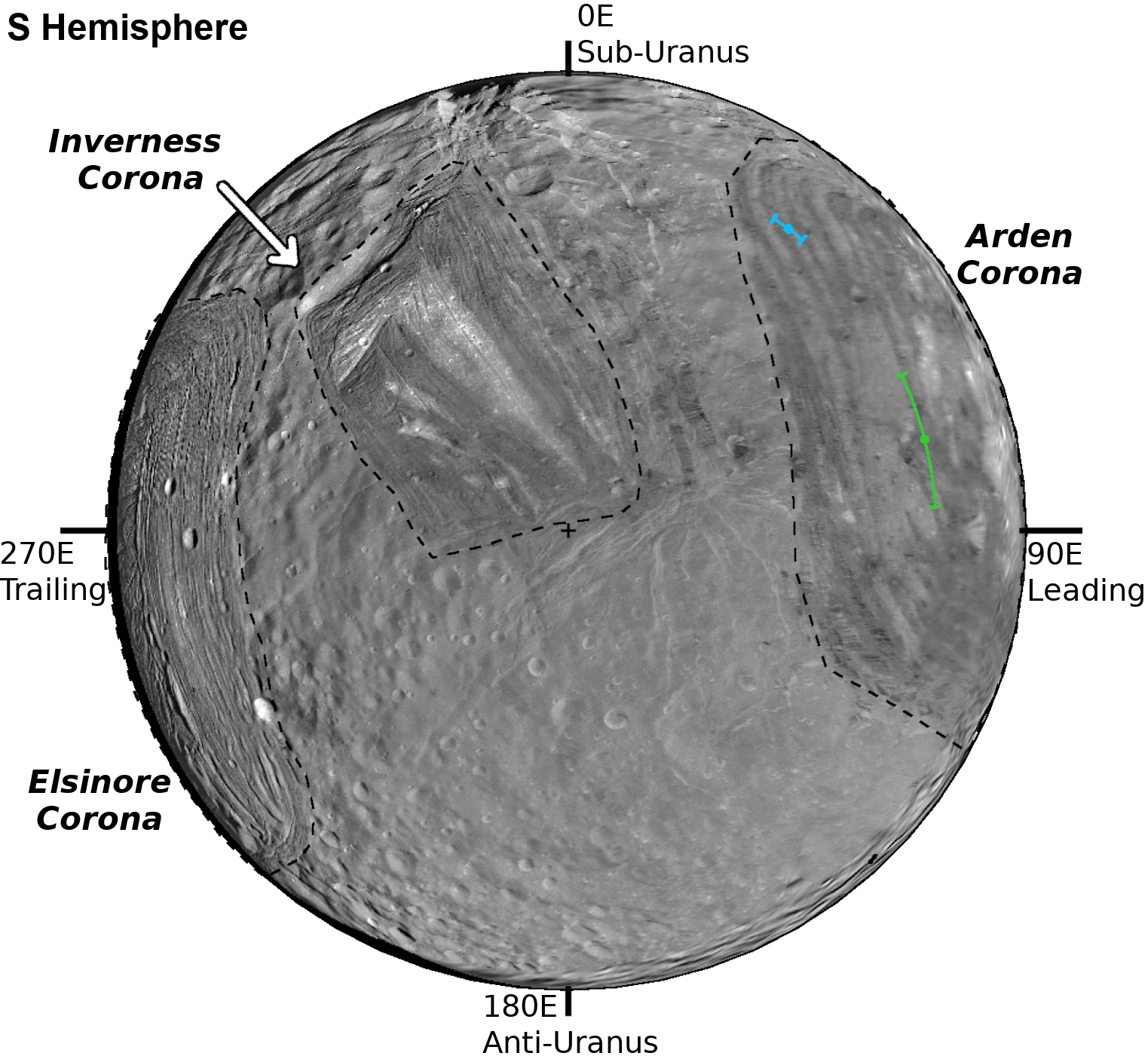
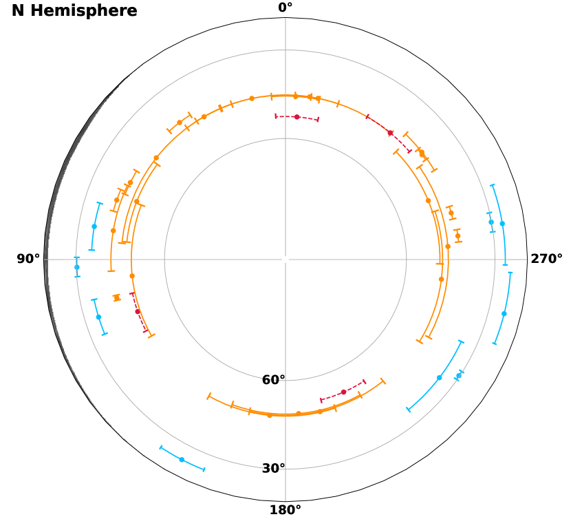
Figure 1: (Left panel): An image mosaic of Miranda’s southern hemisphere from imaging by Voyager 2 in 1986. We use an orthographic projection centered on the south pole, using the Miranda mosaic produced by Schenk & Moore (2020). The ‘coronae’ are regions heavily modified by tectonic activity and possessing intriguing patches of high-albedo material. Only two of the disk-integrated spectra in our dataset were observed with sub-observer latitudes on the southern hemisphere: UT990607, green (Bauer et al., 2002) and UT000907, blue (Cartwright et al., 2018). Errorbars in longitude represent the range of sub-observer longitudes covered during the duration of that observation. (Right panel): All other spectra in our dataset observed Miranda’s northern hemisphere, which was in darkness at the time of the Voyager flyby and has no imaging data available. Orange spectra were observed with TripleSpec, blue spectra were observed with SpeX, and red spectra were observed with GNIRS. Longitudes appear to increase in opposite directions as seen from the north and south poles, so we chose to orient the 0°meridian at the top of the figure in both panels.

Miranda is the smallest of the five classical Uranian satellites. With a radius of $\sim$ 234 km, it is intermediate in size between the Saturnian moons Mimas and Enceladus. Prior to the Voyager 2 flyby of Uranus in 1986, Miranda was expected to possess a surface similar to Mimas (heavily cratered, with minimal to no evidence of geological activity). However, imaging of Miranda’s southern hemisphere collected by Voyager 2 revealed an icy body where three large regions of its surface appeared to be geologically young (called “coronae”), while other regions appeared to be ancient and heavily cratered (Figure 1)(Smith et al., 1986; Greenberg et al., 1991; Schenk & Moore, 2020). The coronae are bounded by large tectonic fault systems, and both Arden and Inverness Corona possess patches of high albedo material that might represent deposits of fresher H₂O ice. At the time, the incongruity between such a small icy body possessing complex tectonic and geological surface features led to the suggestion that Miranda had been disrupted into large chunks after a giant impact and subsequently reaccreted (Smith et al., 1986; Janes & Melosh, 1988). Later work suggests that Miranda’s bizarre coronae instead represent the surface expression of internal upwelling from low order convection (e.g. Pappalardo et al., 1997; Hammond & Barr, 2014), likely with tidal interactions from orbital resonances as a heat source. Crater counts suggest that the coronae are geologically young (0.1 – 1 Gyr, Zahnle et al. (2003); Kirchoff et al. (2022)), and Miranda’s larger neighbor Ariel also displays a relatively young surface, implying that Miranda and Ariel have both experienced complex geological histories.

Furthermore, it has previously been noted that Miranda’s large scale geology is reminiscent of the similarly sized active ocean world Enceladus, such as the presence of three regions of heavily tectonized terrain at the south pole and near the centers of the leading and trailing hemispheres, interspersed with heavily cratered ancient terrain (Pappalardo & Schubert, 2013; Beddingfield & Cartwright, 2020). Miranda is not currently in an orbital resonance that should produce significant internal heating, so the retention of an Enceladus-like subsurface ocean over geological timescales is unlikely (Hussmann et al., 2006; Castillo-Rogez et al., 2023). However, the surface geology indicates that Miranda likely experienced one or more significant heating events in the past (Beddingfield et al., 2015; Schenk & Moore, 2020; Beddingfield et al., 2022), and the apparent youthfulness of the coronae suggests that these events may have been geologically recent.

1.2 H₂O and CO₂ ice

The presence and spectral properties of H₂O ice on the Uranian satellites have been discussed at length in prior work (Brown & Cruikshank, 1983; Brown & Clark, 1984; Grundy et al., 1999; Bauer et al., 2002; Grundy et al., 2003, 2006; Cartwright et al., 2015, 2018, 2020a; DeColibus et al., 2022). We therefore give only a brief overview in this section. The surfaces of the Uranian satellites are characterized primarily by their lower albedos in comparison to similarly sized Saturnian satellites. These low albedos are attributed to a dark, spectrally neutral component (often assumed to be carbonaceous in nature) mantling or intermixed with the icy regolith. This dark material effectively erases the 1.04-$\mu$m and 1.25-$\mu$m H₂O ice bands and substantially decreases the depth of the 1.5-$\mu$m and 2.0-$\mu$m absorption band complexes. The four largest Uranian satellites show leading/trailing asymmetries in the strength of their H₂O ice bands, likely due to a combination of magnetospheric irradiation and impact gardening. Miranda does not show a leading/trailing asymmetry in the strength of its H₂O ice bands, although it possesses an anti-Uranus/sub-Uranus asymmetry instead (Cartwright et al., 2018; DeColibus et al., 2022).

Previous work reported the presence of CO₂ ice on the four largest Uranian satellites (Grundy et al., 2003, 2006; Cartwright et al., 2015, 2022). This CO₂ ice is identified via a triplet of narrow absorption features at 1.966, 2.012, and 2.070 µm. Weaker CO₂ ice absorption bands are also present at 1.543, 1.578, and 1.609 µm, mostly on Ariel, which has the strongest CO₂ ice signatures. These CO₂ ice deposits are thought to be present primarily in pure deposits and not intermixed with the H₂O ice regolith. Furthermore, a forbidden $2\nu_{3}$ overtone mode of CO₂ exhibits an absorption feature near 2.134 $\mu$m (Bernstein et al., 2005), which only appears in molecular mixtures of CO₂ ice in H₂O ice and/or methanol (CH₃OH) ice, might be present on Ariel (Cartwright et al., 2022) and Umbriel (Cartwright et al., 2023).

The distribution of CO₂ ice on the Uranian moons shows both longitudinal and planetocentric trends. The CO₂ absorption features are stronger on moons closer to Uranus, and on each individual moon, the CO₂ ice bands are stronger on their trailing hemispheres. This information supports an interpretation in which CO₂ molecules are produced in situ by magnetospheric bombardment of the trailing hemispheres of the Uranian satellites. Irradiation of the H₂O ice and carbonaceous compounds in the regolith dissociates molecules that then recombine into CO₂, potentially with CO as an intermediary product (Cartwright et al., 2022). Plasma densities in the magnetosphere are higher closer to Uranus, implying that a radiolytic production process of CO₂ should plausibly be more effective on moons closer to the planet. This assertion is supported by the relative strength of the CO₂ absorption features across the various satellites, as the CO₂ signature is strongest on Ariel and weakest on Oberon, which spends part of its orbit outside of the Uranian magnetosphere (Ness et al., 1986). Thermodynamical modeling work indicates that radiolytically generated CO₂ molecules should preferentially accumulate in cold traps at low latitudes on the trailing hemispheres of each satellite, assuming radiolytic production is greater on their trailing sides (Grundy et al., 2006; Sori et al., 2017). More recent telescope observations show a decrease in the strength of the CO₂ ice bands on Ariel at higher sub-observer latitudes, consistent with the hypothesis that CO₂ cold traps are concentrated at low latitudes (Cartwright et al., 2022).

Miranda is the innermost of the five classical satellites, and therefore, it should be the most irradiated by charged particles trapped in the Uranian magnetosphere. Miranda presumably possesses the same “raw ingredients” in its regolith (carbonaceous compounds and H₂O ice) as the other Uranian satellites (Brown & Clark, 1984), unless Miranda formed from a different mix of materials, possibly as a consequence of the Uranus-tilting event (Rufu & Canup, 2022; Salmon & Canup, 2022). It therefore follows that radiolytic production of CO₂ molecules should also be occurring on Miranda, and it may also maintain deposits of CO₂ ice like the other Uranian moons. However, previous spectroscopic studies of Miranda have not detected CO₂ ice on its surface (Bauer et al., 2002; Gourgeot et al., 2014; Cartwright et al., 2018). These prior studies were somewhat limited by low signal-to-noise ratio (S/N) reflectance spectra in the 2.0-$\mu$m region, due to several observational limitations. Miranda is much fainter than the other Uranian moons at K${}_{mag}\sim 15$, compared to K${}_{mag}\sim$12-13 for the larger moons. The CO₂ ice absorption features of interest are narrow, requiring higher spectral resolving power and therefore lower S/N per spectral pixel. The CO₂ ice absorption bands are superimposed on the wide and deep 2.0-$\mu$m H₂O ice absorption band, and the CO₂ ice bands are also in a region of strong telluric absorption from CO₂ in the Earth’s atmosphere. Although the spectral signature of atmospheric CO₂ is distinctly different than that of crystalline CO₂ ice (e.g., Hansen, 1997), telluric contamination introduces additional uncertainty into the spectral data points. These prior observations established CO₂ ice band depth upper limits of 5% of the continuum on Miranda. Therefore, if CO₂ ice is present, it is much less abundant on Miranda than on Ariel (Cartwright et al., 2018). Additionally, CO₂ molecules in a molecular mixture with H₂O ice might be present and detectable prior to escaping Miranda’s low gravity. Investigating whether Miranda spectra show the 2.13-$\mu$m $2\nu_{3}$ overtone band could help determine whether regolith-mixed CO₂ is present. The primary questions relating to CO₂ that this work aims to answer are therefore twofold: (1) do concentrated CO₂ ice deposits exist on Miranda’s surface at low abundances, and (2) is there evidence for CO₂ in a molecular mixture with H₂O ice in the regolith?

1.3 The 2.2-$\mu$m feature

Some icy bodies show evidence for weak absorption features in the region between 2.18 and 2.26 µm, which we refer to generically as the 2.2-$\mu$m feature. The 2.2-$\mu$m feature on icy bodies has frequently been attributed to ammonia (NH₃)- or ammonium (NH₄)-bearing compounds (which we will collectively refer to as NH-bearing). NH-bearing species are of significant geological and astrobiological interest, as NH₃ is a potent antifreeze, capable of reducing the freezing point of liquid H₂O by nearly 100 K if present in sufficiently high abundances (Kargel, 1992). This makes NH₃ an important compound for enabling internal activity and extending the retention of subsurface oceans on icy bodies. NH₄-bearing salts and minerals are much less effective than NH₃ in an antifreeze role (Neveu et al., 2017), but indicate the past presence of NH₃, and NH${}_{4}^{+}$ is readily produced by irradiation of H₂O + NH₃ ice mixtures (Moore et al., 2003, 2007).

Despite the expected ubiquity of NH₃-bearing compounds in the solar nebula at intermediate to large heliocentric distances (Lewis, 1971), the 2.2-$\mu$m feature is not observed in the spectra of many icy bodies, possibly because of removal by irradiation over short geological timescales. In the case of Miranda, NH₃ may be effectively removed from its surface in timescales as short as $<$10⁶ years (Moore et al., 2007). Detection of the 2.2-$\mu$m feature could therefore imply that NH₃-bearing compounds have been exposed or emplaced in the geologically recent past, either via endogenic processes such as tectonism and cryovolcanism or via mass wasting and impact events. The possibility of recent endogenic activity on Miranda is particularly tantalizing given the apparent youth of some regions of its heavily modified surface, discussed in §1.1, and past reports of a weak 2.2-$\mu$m absorption feature (Bauer et al., 2002).

1.3.1 The 2.2-$\mu$m feature on other icy bodies

One of the icy bodies that shows the most consistent evidence of a 2.2-$\mu$m feature is Charon (e.g., Brown & Calvin, 2000; Dumas et al., 2001). Prior to the New Horizons flyby of the Pluto system, ground-based spectroscopic studies investigated the 2.2-$\mu$m feature on Charon in detail, finding evidence for longitudinal variation in the strength and wavelength position of the 2.2-$\mu$m band (Cook et al., 2007; Merlin et al., 2010; DeMeo et al., 2015; Holler et al., 2017). Data acquired during the New Horizons flyby further confirmed the band’s presence on Charon and an apparent spatial association with impact craters (Grundy et al., 2016; Cook et al., 2018; Dalle Ore et al., 2018). Dalle Ore et al. (2019) and Cruikshank et al. (2019) found the 2.2-$\mu$m band to be present near geologically young surface features on Pluto that also exhibit spectral evidence of H₂O ice, strengthening a possible association with emplacement of NH-bearing compounds via cryovolcanism/internal activity. In contrast, Cook et al. (2018) reported on strong 2.2-$\mu$m bands on Pluto’s minor moons Nix and Hydra, which are too small to support internal geological activity.

In addition to the Uranian satellites and icy bodies in the Pluto system, detection of weak 2.2-$\mu$m features also have been reported on Enceladus (Emery et al., 2005; Verbiscer et al., 2006), Tethys (Verbiscer et al., 2008), Orcus (Carry et al., 2011), Haumea and its satellite Hi’iaka (Barkume et al., 2006), and Quaoar (Jewitt & Luu, 2004). NH₄-bearing species have been reported on Ceres (King et al., 1992; de Sanctis et al., 2016; Raponi et al., 2019) and comets (Poch et al., 2020), and the 2.2-$\mu$m feature on Charon and the smaller moons in the Pluto system has been attributed to NH₄Cl (Cook et al., 2018, 2023). However, a 2.2-$\mu$m absorption band is not exclusive to NH-bearing species. Other minerals and compounds can also exhibit absorption in this region, including many phyllosilicates (hydrated silicates) with an Al-OH bond (Clark et al., 1990). Certain types of phyllosilicates are also prone to incorporating NH₄ into their composition through cation exchange processes (Bishop et al., 2002; Berg et al., 2016).

1.3.2 The 2.2-$\mu$m feature on the Uranian satellites

Bauer et al. (2002) was the first work to identify a 2.2-$\mu$m feature on any of the Uranian satellites, reporting a relatively strong band on Miranda (plotted in green in the left panel of Figure 2). The authors reported an absorption band similar to that of the 2.21-$\mu$m feature on Charon, and attributed it to ammonia hydrate (NH${}_{3}\cdot n$H₂O). At the time, Miranda was only the third icy body on which a 2.2-$\mu$m band had been reported. However, subsequent spectral studies of Miranda (Gourgeot et al., 2014; Cartwright et al., 2018) did not find conclusive evidence of a 2.2-$\mu$m absorption feature, leaving its existence an open question.

From visual inspection, Cartwright et al. (2018) noted weak absorption features in the 2.2-$\mu$m region on Ariel, Umbriel, Titania, and Oberon. The authors followed up with a detailed study of 2.2-$\mu$m features on Ariel in Cartwright et al. (2020b), finding several different absorption bands associated with NH₃- and NH₄-bearing compounds, which varied in strength and band center in different spectra. They found no large scale longitudinal patterns in these variations. They compared these bands with NH₃ hydrates (NH${}_{3}\cdot n$H₂O, 2.215 µm), flash frozen NH₃-H₂O solutions (2.210 µm), NH₃ ice (2.238 µm), and an NH₄-bearing species (possibly (NH₄)₂CO₃, 2.181 µm). Some of these bands have been reported to show double absorptions and wavelength shifts based on temperature and the ratio of NH₃ to H₂O (Moore et al., 2007), further complicating the identification of individual compounds.

Further research has also presented evidence of similar weak absorption features in the 2.2-$\mu$m region on Umbriel (Cartwright et al., 2023). However, the surface of Umbriel is ancient and heavily cratered (within the resolution limits of Voyager 2 imaging), lacking evidence of resurfacing driven by endogenic activity. The presence of 2.2-$\mu$m bands in spectra of Umbriel raises important questions about the presumed short lifetime of NH-bearing species on the surfaces of the Uranian moons (Moore et al., 2007), and also raises the possibility that other species such as phyllosilicate minerals or nitrogen-bearing organics contribute to the 2.2-$\mu$m band, at least on Umbriel.

2 Observations

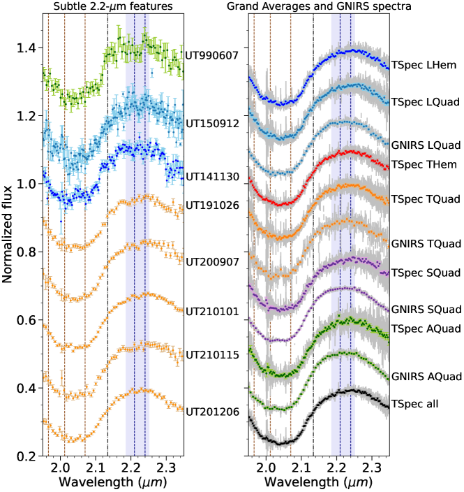
Figure 2: (Left panel): Examples of Miranda spectra displaying weak absorption features around 2.2 µm. The green spectrum is the (unbinned) spectrum reported in Bauer et al. (2002). The two blue spectra were obtained with SpeX in the PRISM and SXD configuration (unbinned and binned by 10 pixels, respectively). The orange spectra are spectra from individual nights with TripleSpec (binned by 30 pixels). The text next to each spectrum indicates the date of observation in format UTYYMMDD (e.g. UT200907 = UT 2020-09-07). This UTYYMMDD date format is used throughout this work. Vertical lines are placed at the expected wavelengths for the absorption features studied in this work: brown lines at 1.966, 2.012, and 2.070 $\mu$m for the CO₂ ice triplet, a black line at 2.134 $\mu$m for a feature associated with molecular mixtures including CO₂ ice, a blue line at 2.21 $\mu$m for NH₃-hydrates, and a blue line at 2.24 $\mu$m for crystalline NH₃ ice. The shaded region indicates the wavelength range measured for the 2.2-$\mu$m band in this work. (Right panel): The GNIRS spectra and TripleSpec quadrant and hemisphere grand average spectra originally reported in DeColibus et al. (2022). Colored points are binned by 15 pixels, and the gray error bars are presented at the native resolution of the data.

Table 1: Miranda Observations

Observing PI	Year(s)	Latitude(s)	Telescope	Instrument	Resolving power	Nspec	Reference
		°N, Sub-Earth			($\lambda/\Delta\lambda$)
Bauer	1999	-36.5	UKIRT	CGS4	$\sim$200	1	Bauer et al. (2002)
Rivkin	2000	-35.4	IRTF	SpeX SXD	$\sim$750	1	Cartwright et al. (2018)
Gourgeot	2012	21.4	IRTF	SpeX SXD	$\sim$750	2	Gourgeot et al. (2014)
Cartwright	2014–2017	24.7 – 36.7	IRTF	SpeX SXD	$\sim$750	2	Cartwright et al. (2018)
Cartwright	2014–2017	24.7 – 36.7	IRTF	SpeX PRISM	$\sim$95	5	Cartwright et al. (2018)
DeColibus	2019–2021	42.3 – 50.4	ARC 3.5m	TripleSpec	$\sim$3500	18	DeColibus et al. (2022)
DeColibus	2020	47.2 – 49.6	Gemini N	GNIRS XD	$\sim$1130	2	DeColibus et al. (2022)
DeColibus	2021	53.3 – 53.8	Gemini N	GNIRS XD	$\sim$750	2	DeColibus et al. (2022)

Note. — A table of basic information about the collection of Miranda spectra analyzed in this work. For more details, we direct the reader to the listed references.

We analyzed 33 disk-integrated near-IR spectra of Miranda, covering the wavelengths between $\sim$0.95 – 2.45 µm, summarized in Table 1. Eighteen of these spectra were obtained with the TripleSpec spectrograph on the ARC 3.5-meter telescope at Apache Point Observatory, four spectra were acquired with GNIRS on the 8.1-meter Gemini North telescope on Maunakea, and ten spectra were observed with SpeX on NASA’s 3-meter Infrared Telescope Facility (IRTF) on Maunakea. For information on the acquisition and data reduction of the TripleSpec and GNIRS spectra, we refer the reader to DeColibus et al. (2022), while for the SpeX spectra, we refer the reader to Gourgeot et al. (2014) and Cartwright et al. (2018). Table 1 lists the average spectral resolving power ($R=\lambda/\Delta\lambda$) of data acquired with each instrument configuration. Two spectral data points can be placed across the narrow CO₂ absorption bands at R$\sim$750, so they should be detectable in spectra acquired at this or higher spectral resolution. All of the spectra except those acquired with the SpeX PRISM configuration have sufficient spectral resolution to at least detect the CO₂ bands, and the 2.2-$\mu$m feature is broad enough to be detectable in the PRISM spectra. The dataset also includes seven TripleSpec ‘grand average’ (GAvg) spectra, which were constructed as averages of all TripleSpec exposures in which the sub-observer longitude fell within defined ranges. These are the leading, trailing, sub-Uranus, and anti-Uranus quadrants; the leading and trailing hemispheres; and all exposures regardless of longitude. These grand average spectra and the GNIRS spectra are plotted in Figure 2.

We also modified one spectrum in the above dataset. The GNIRS anti-Uranus quadrant spectrum from UT211121 displayed a high S/N, but the error bars on the spectrum were uniformly overestimated compared to what might reasonably be expected given the apparent S/N of the data and when compared to the other GNIRS spectra obtained in similar conditions (see Figure 5 of DeColibus et al. (2022)). In order to calculate more accurate uncertainties for each data point while retaining wavelength-dependent error information, such as increased uncertainties in regions of heavy telluric absorption, we adopted a procedure similar to that of Holler et al. (2022). We calculated the standard deviation of the flux values and the mean of the original uncertainty values in a region of the spectrum that could reasonably be described by a flat continuum (1.70 – 1.80 µm). Division of these two quantities results in the factor by which the errors in the original spectrum were overestimated, approximately $\sim$3.32. Division by this factor resulted in a more accurate estimate of the uncertainties for the data points in that spectrum, and the corrected spectrum was used for all analyses presented here.

Finally, we also digitized the spectrum of Miranda’s leading hemisphere published in Bauer et al. (2002), in which the presence of a 2.2-$\mu$m feature was first reported. The K-band portion of this spectrum was acquired on 1999 June 7 with the CGS4 spectrograph on the 3.8-meter UKIRT telescope on Maunakea. We utilized timing and observing geometry information provided in Table 1 of Bauer et al. (2002), combined with the JPL HORIZONS ephemeris service, to derive a central sub-observer longitude of 75.7°E and a latitude of 36.5°S. For further information on the Bauer et al. spectrum, we direct the reader to the original work. This spectrum and one SpeX SXD spectrum acquired in 2000 at latitude 35.4°S are the only two southern hemisphere spectra in our data set. All other spectra were acquired at northern sub-observer latitudes (Figure 1).

3 Spectral Analysis

We measured the integrated band areas of three CO₂ ice bands in the Miranda spectra. The CO₂ ice bands at 1.966, 2.012, and 2.070 $\mu$m are referred to in this work as the “CO₂ ice triplet” as a whole and as bands 1, 2, and 3 individually. We also measured the integrated band areas and fractional band depths of a subtle feature at 2.13-$\mu$m and the 2.2-$\mu$m absorption band.

3.1 Band measurement methods

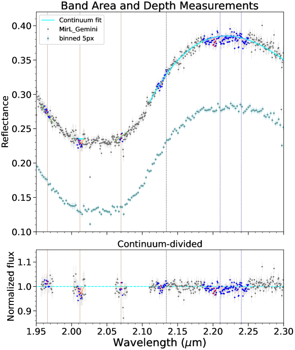
Figure 3: A demonstration of the band area and depth measurement process for the CO₂ ice triplet and the 2.13-$\mu$m and 2.2-$\mu$m bands, using the GNIRS leading hemisphere spectrum of Miranda from UT201008. The data points over which the band areas are integrated are marked in blue, the points where the band depth is measured in red, continuum fits are cyan lines, and Gaussian band fits are orange lines. A copy of the spectrum plotted with an offset has been binned by five pixels (turquoise points). Vertical lines are the same as in Figure 2.

Table 2: Absorption band wavelengths

Band name	Left continuum	Band width	Right continuum	Center
	($\mu m$)	($\mu m$)	($\mu m$)	($\mu m$)
CO2 2$\nu_{1}$+$\nu_{3}$ (Band 1)	1.957 – 1.962	1.962 – 1.969	1.969 – 1.974	1.966
CO2 $\nu_{1}$+2$\nu_{2}$+$\nu_{3}$ (Band 2)	2.002 – 2.008	2.008 – 2.015	2.015 – 2.020	2.012
CO2 4$\nu_{2}$+$\nu_{3}$ (Band 3)	2.062 – 2.068	2.068 – 2.073	2.073 – 2.079	2.070
2.13-$\mu$m band	$\cdots$	2.121 – 2.135	$\cdots$	2.134
2.2-$\mu$m band	$\cdots$	2.186 – 2.251	$\cdots$	2.21

Note. — We tabulate the wavelengths we used to define the band continua, widths, and centers. For the 2.13-$\mu$m and 2.2-$\mu$m band, the continuum was fit with the 3rd degree polynomial fit described in the text. ‘Center’ refers to the expected central wavelength of the absorption band.

Our band area and depth measurements were conducted with the same analysis routine described in DeColibus et al. (2022), modified for use on the CO₂ ice bands, 2.13-$\mu$m band, and 2.2-$\mu$m band. This routine is a Python implementation of the technique described in Cartwright et al. (2015, 2018), which used a modified version of the SARA band analysis routine originally developed for asteroid spectra (Lindsay et al., 2015). The band analysis code generates a sample spectrum, drawing from a Gaussian distribution where the mean and standard deviation are the flux and errors of the input spectrum, respectively. The absorption bands of interest (Table 2) are measured by drawing a line between the continuum on either side of the absorption band, normalizing by this line, and integrating the area inside the absorption band with the trapezoidal rule. The CO₂ ice absorption bands are further fit by a Gaussian function to determine the band centers, from which the depths of the bands are measured using the points within 0.0005 $\mu$m of the center of the band. This choice of band width for the depth measurement was determined from inspection of the CO₂ ice bands in spectra of Ariel. This process is demonstrated visually using a GNIRS spectrum of Miranda’s leading hemisphere in Figure 3. To calculate the uncertainties on each measurement, this entire sample spectrum generation and measurement process is repeated 20,000 times, which is a number of samples consistent with other Monte Carlo type approaches to measurements of band parameters (e.g. Lindsay et al., 2015; Cartwright et al., 2015). The mean and standard deviation of the measurements of this ensemble are reported as the final band measurements for each individual spectrum in Table 3. For each spectrum, we also summed the band area measurements for the three CO₂ bands into a total CO₂ band area. Due to inadequate spectral resolution, we did not measure the CO₂ ice triplet for the Bauer et al. (2002) spectrum nor the SpeX spectra collected in PRISM mode.

The process for the 2.13-$\mu$m and 2.2-$\mu$m bands was slightly different. Instead of measuring the continuum by drawing a line on either side of the absorption band, the continuum is defined with a third-order polynomial curve, fit to the data points between 2.11 – 2.19 $\mu$m and 2.23 – 2.34 µm. The region between 2.19 – 2.23 $\mu$m is not used in the fit to avoid the influence of any possible 2.2-$\mu$m absorption features. The spectrum is divided by this continuum model, and the integrated band areas and fractional band depths are measured in wavelength ranges corresponding to the absorption bands of interest. We used a Gaussian fit procedure similar to the one used for the CO₂ ice triplet to measure the central wavelength and depth of the 2.13-$\mu$m band. However, for the 2.2-$\mu$m band, the potential presence of multiple absorptions across the 2.18 – 2.25 $\mu$m range would be poorly fit by a Gaussian model. We instead binned the spectrum by five pixels and chose the lowest data point in the continuum-divided band as the central wavelength. The fractional band depth for the 2.2-$\mu$m band are measured using the mean of the unbinned, native resolution data points within $\pm$0.002 $\mu$m of this central wavelength. This process was also iterated 20,000 times for each spectrum, and the mean and standard deviation of the measurements for each individual spectrum are reported in Table 4.

3.2 Means, ratios, and sinusoidal models

We calculated the mean band parameters, using the final measurements of each of the spectra that fall within given sub-observer longitude quadrants and hemispheres. We also calculated a set of mean measurements that included all spectra from individual nights (i.e. not including the TripleSpec grand averages). These mean measurements are tabulated in Table 5 and plotted in Figure 5. Figure 5 also includes the band measurements from the quadrant and hemisphere-averaged TripleSpec grand average spectra and the GNIRS spectra for comparison to the mean measurements.

We took the ratios of the mean band measurements between opposing quadrants and hemispheres (Table 6) to test whether a band was statistically stronger on one quadrant/hemisphere versus the other, as might be expected from exogenic effects. We did not find statistically significant ($\geq 2\sigma$) departures from a ratio of unity for any of the measurements or quadrant/hemisphere pairs.

We fit our band measurements to a sinusoidal model to search for longitudinal variation, with the period fixed at 2$\pi$ to represent one rotation of the body. This approach has previously been used for Miranda and the other Uranian satellites (Grundy et al., 2006; Cartwright et al., 2015, 2018; DeColibus et al., 2022) and we direct the reader to those works for further information. We also applied an F-test to the sinusoidal models, which allows us to discern whether the sinusoidal model fit is a statistically significant better fit compared to the null hypothesis (no variation with sub-observer longitude). The sinusoidal models and F-tests are tabulated in Table 7.

3.3 Hapke-Mie modeling

We constructed spectral models in order to investigate possible absorption features in the 2.2-$\mu$m region. We chose a hybrid Hapke-Mie model using intimate (particulate) mixing, as has previously been done for the Uranian satellites (Cartwright et al., 2015, 2018, 2020a). The Hapke-Mie model utilizes Mie theory to calculate the single scattering albedo of individual particles, which are then incorporated into the standard Hapke model equations. We assume an isotropic single scattering phase function which does not depend on wavelength. The Hapke-Mie approach accounts for the effects of grain sizes approaching wavelength, such as diffraction and Rayleigh scattering (Clark et al., 2012). However, at some particle sizes the exact Mie solution can introduce periodic resonance artifacts in the resulting spectrum. We mitigate this effect by calculating the average albedo of a spread of sizes around the specified grain size, typically with a 10% spread in particle diameter.

As has been noted by previous studies, Miranda’s spectrum is consistent with a surface composition incorporating H₂O ice and a dark, spectrally neutral component, such as amorphous carbon (Brown & Clark, 1984; Bauer et al., 2002; Gourgeot et al., 2014). We scaled our observed spectra to a geometric albedo of 0.434 at 1.72 $\mu$m (from Figure 7 of Karkoschka (2001)). For our models, we used the optical constants of crystalline H₂O ice at 80 K from Mastrapa et al. (2008) and optical constants of amorphous carbon (sample BE1) from Rouleau & Martin (1991).

We found that a small percentage of intimately mixed sub-micron H₂O ice grains assist in reproducing Miranda’s spectrum. The central wavelength of the 2.0-$\mu$m H₂O ice band is shifted to slightly longer wavelengths, the continuum in the 2.2-$\mu$m region is low compared to the 1.8-$\mu$m continuum, and the blue slope from 2.3 – 2.5 $\mu$m is steeper than in typical H₂O ice models of larger diameter grains. These characteristics are consistent with the presence of sub-micron H₂O ice grains (Clark et al., 2012), and previous studies have suggested that the regoliths of the Uranian satellites show a ‘fluffy’ structure and evidence of the presence of tiny grains with sub-micron diameters, likely composed of H₂O ice (Afanasiev et al., 2014; Cartwright et al., 2020a).

We adjusted individual parameters (grain size and mixing ratio) of the model components until we found a fit that generally reproduced the continuum shape of our spectra between 2.0 – 2.4 µm. We specifically attempted to be agnostic regarding any possible absorption features in the 2.2-$\mu$m region, as the possible presence of several overlapping weak bands made identifying a ‘clean’ continuum difficult. because of degeneracies between model parameters, our spectral models provide useful but non-unique solutions. We also experimented with the addition of small amounts of other compounds (such as NH₃ ice) to study their effects on the resulting spectra. This analysis is described further in §5.

4 Results

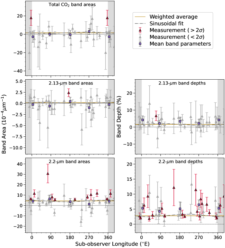
Figure 4: Band area and depth measurements for each Miranda spectrum in this work, with 1$\sigma$ error bars. Band area and depth measurements that are not statistically significant ($<$2$\sigma$ from zero) are plotted as gray triangles, while those that are $\geq$2$\sigma$ are plotted as red triangles. Quadrant-averaged mean band parameters (Table 5) are plotted as purple squares. The gray shaded regions on either side of each plot represent overlapping longitudes. Data points are duplicated in these regions to better visualize possible sinusoidal variations with longitude. The weighted average and sinusoidal fit to all spectra for each measurement are plotted as golden horizontal lines and gray dot-dashed lines, respectively. Top left: Total band areas for the CO₂ ice triplet measurements (sum of the 1.966, 2.012, and 2.070 $\mu$m band areas). Center row: Band area measurements (left panel) and band depths (right panel) for the 2.13-$\mu$m band. Bottom row: Same as the center row, but for the 2.2-$\mu$m band.

Figure 5: Band area and depth measurements for the high S/N Miranda spectra (GNIRS spectra and the TripleSpec quadrant/hemisphere grand average spectra), along with the same mean measurements (purple squares) plotted in the previous figure. All error bars represent 1$\sigma$ uncertainties. The weighted average and sinusoidal fits use the mean band measurements.

Table 3: CO₂ triplet band measurements

UT Date	Long.	Lat.	Integrated band area			Total CO2	$>2\sigma$	Band depths
			1.966-$\mu$m	2.012-$\mu$m	2.070-$\mu$m	band area	total	1.966-$\mu$m	2.012-$\mu$m	2.070-$\mu$m
	(°E)	(°N)	(10${}^{-4}\mu$m)	(10${}^{-4}\mu$m)	(10${}^{-4}\mu$m)	(10${}^{-4}\mu$m)	area?	(%)	(%)	(%)
UT210115	11.8	47.2	$-2.32\pm 5.07$	$-2.60\pm 7.33$	$0.08\pm 1.97$	$-4.84\pm 9.13$	No	$-0.00\pm 0.12$	$0.01\pm 0.16$	$0.04\pm 0.08$
UT201229b	29.7	47.2	$-11.33\pm 13.59$	$-1.76\pm 17.21$	$-0.39\pm 3.24$	$-13.48\pm 22.17$	No	$-0.07\pm 0.27$	$0.23\pm 0.32$	$0.09\pm 0.12$
UT000907	36.3	-35.4	$0.51\pm 1.07$	$-0.00\pm 1.91$	$0.64\pm 0.59$	$1.15\pm 2.27$	No	$0.02\pm 0.03$	$0.07\pm 0.04$	$0.03\pm 0.04$
UT191022a	37.7	44.3	$-7.37\pm 14.71$	$-6.94\pm 25.97$	$6.28\pm 4.22$	$-8.03\pm 30.15$	No	$0.08\pm 0.39$	$0.00\pm 0.50$	$0.22\pm 0.16$
UT210101	51.8	47.2	$3.31\pm 2.02$	$-3.14\pm 3.93$	$-1.41\pm 1.10$	$-1.23\pm 4.55$	No	$0.08\pm 0.05$	$0.01\pm 0.10$	$-0.01\pm 0.04$
UT201104	68.7	48.7	$-0.75\pm 3.21$	$-7.18\pm 4.97$	$-1.51\pm 1.38$	$-9.44\pm 6.07$	No	$0.08\pm 0.07$	$-0.06\pm 0.10$	$-0.05\pm 0.05$
UT990607	75.7	-36.5	$\cdots$	$\cdots$	$\cdots$	$\cdots$	No	$\cdots$	$\cdots$	$\cdots$
UT170930	80.2	36.7	$\cdots$	$\cdots$	$\cdots$	$\cdots$	No	$\cdots$	$\cdots$	$\cdots$
UT191104	80.5	43.8	$1.84\pm 3.57$	$\mathbf{7.66\pm 3.72}$	$-0.66\pm 1.38$	$8.84\pm 5.34$	No	$0.08\pm 0.11$	$0.13\pm 0.12$	$0.00\pm 0.05$
UT150912	92.1	30.4	$\cdots$	$\cdots$	$\cdots$	$\cdots$	No	$\cdots$	$\cdots$	$\cdots$
UT200907	96.1	50.4	$2.12\pm 5.72$	$2.38\pm 5.36$	$-3.87\pm 1.85$	$0.63\pm 8.06$	No	$0.07\pm 0.12$	$0.13\pm 0.11$	$-0.04\pm 0.08$
UT171010	107.1	36.1	$\cdots$	$\cdots$	$\cdots$	$\cdots$	No	$\cdots$	$\cdots$	$\cdots$
UT201008g	109.4	49.6	$-0.70\pm 0.98$	$1.84\pm 1.11$	$0.17\pm 0.48$	$1.31\pm 1.56$	No	$-0.01\pm 0.02$	$0.03\pm 0.03$	$0.01\pm 0.03$
UT120926	152.6	21.4	$-6.72\pm 8.24$	$6.31\pm 9.35$	$-0.14\pm 3.53$	$-0.55\pm 12.96$	No	$-0.01\pm 0.19$	$0.14\pm 0.21$	$0.06\pm 0.13$
UT201007	174.2	49.7	$1.88\pm 2.56$	$-1.10\pm 3.87$	$-0.03\pm 1.15$	$0.75\pm 4.78$	No	$0.03\pm 0.07$	$0.05\pm 0.10$	$0.00\pm 0.05$
UT200913	184.9	50.3	$-3.33\pm 5.43$	$-5.83\pm 7.08$	$-1.73\pm 1.94$	$-10.89\pm 9.13$	No	$-0.02\pm 0.12$	$-0.04\pm 0.17$	$0.02\pm 0.07$
UT200930	192.8	49.9	$2.79\pm 2.50$	$3.53\pm 3.78$	$0.09\pm 1.21$	$6.41\pm 4.69$	No	$0.07\pm 0.06$	$0.11\pm 0.08$	$0.03\pm 0.05$
UT211121g	203.7	53.3	$0.45\pm 0.82$	$1.37\pm 1.00$	$0.46\pm 0.52$	$2.28\pm 1.39$	No	$0.01\pm 0.02$	$0.04\pm 0.02$	$0.02\pm 0.02$
UT170925	232.5	36.7	$2.16\pm 3.18$	$-6.70\pm 6.83$	$-2.47\pm 2.36$	$-7.01\pm 7.89$	No	$0.13\pm 0.09$	$-0.01\pm 0.17$	$-0.03\pm 0.11$
UT150911	236.2	30.4	$\cdots$	$\cdots$	$\cdots$	$\cdots$	No	$\cdots$	$\cdots$	$\cdots$
UT120925	256.1	21.4	$1.04\pm 6.31$	$1.87\pm 7.57$	$0.11\pm 4.34$	$3.02\pm 10.77$	No	$0.09\pm 0.15$	$0.07\pm 0.17$	$0.06\pm 0.15$
UT201013	262.8	49.5	$2.59\pm 2.51$	$-5.23\pm 4.03$	$-0.19\pm 1.03$	$-2.83\pm 4.86$	No	$0.05\pm 0.05$	$-0.06\pm 0.09$	$0.03\pm 0.04$
UT201206	274.6	47.7	$1.79\pm 2.80$	$5.01\pm 3.46$	$-0.80\pm 1.14$	$6.00\pm 4.60$	No	$0.03\pm 0.06$	$0.10\pm 0.08$	$-0.02\pm 0.05$
UT141130	279.4	24.7	$6.22\pm 3.80$	$3.88\pm 6.61$	$1.89\pm 2.40$	$11.99\pm 8.00$	No	$0.11\pm 0.15$	$0.14\pm 0.16$	$0.06\pm 0.15$
UT150917	280.3	30.2	$\cdots$	$\cdots$	$\cdots$	$\cdots$	No	$\cdots$	$\cdots$	$\cdots$
UT191013a	285.7	44.6	$3.95\pm 8.43$	$8.51\pm 8.52$	$4.64\pm 3.15$	$17.10\pm 12.39$	No	$0.12\pm 0.20$	$0.19\pm 0.18$	$0.13\pm 0.13$
UT200912	292.4	50.3	$-3.68\pm 5.02$	$-2.42\pm 6.16$	$0.89\pm 1.75$	$-5.21\pm 8.14$	No	$-0.00\pm 0.10$	$0.01\pm 0.14$	$0.01\pm 0.08$
UT191026	308.2	44.2	$4.07\pm 3.78$	$-2.24\pm 6.00$	$-0.60\pm 1.75$	$1.23\pm 7.31$	No	$0.15\pm 0.11$	$0.03\pm 0.15$	$0.07\pm 0.06$
UT201230g	320.4	47.2	$-7.25\pm 2.23$	$5.07\pm 2.72$	$0.83\pm 0.83$	$-1.35\pm 3.62$	No	$-0.07\pm 0.06$	$\mathbf{0.14\pm 0.05}$	$0.02\pm 0.04$
UT201229a	348.6	47.2	$-2.41\pm 8.91$	$-20.80\pm 15.85$	$3.28\pm 3.01$	$-19.93\pm 18.43$	No	$0.09\pm 0.24$	$-0.24\pm 0.29$	$0.14\pm 0.15$
UT210105	351.5	47.2	$1.06\pm 2.48$	$2.50\pm 3.52$	$-0.82\pm 1.07$	$2.74\pm 4.44$	No	$0.06\pm 0.05$	$0.07\pm 0.08$	$-0.01\pm 0.04$
UT211106g	355.4	53.8	$0.32\pm 0.56$	$1.13\pm 0.64$	$0.17\pm 0.34$	$1.62\pm 0.91$	No	$0.02\pm 0.01$	$0.04\pm 0.02$	$0.01\pm 0.01$
UT201212	356.4	47.5	$7.79\pm 4.94$	$11.04\pm 6.14$	$-0.93\pm 2.58$	$\mathbf{17.90\pm 8.29}$	Yes	$\mathbf{0.21\pm 0.10}$	$0.20\pm 0.14$	$-0.00\pm 0.12$
GAvg SQ	3.8	47.0	$1.48\pm 1.58$	$0.12\pm 2.43$	$-0.65\pm 0.72$	$0.95\pm 2.99$	No	$0.05\pm 0.03$	$0.02\pm 0.06$	$-0.02\pm 0.03$
GAvg LQ	79.1	47.2	$1.43\pm 1.74$	$-0.21\pm 2.75$	$-1.32\pm 0.80$	$-0.10\pm 3.35$	No	$0.05\pm 0.04$	$0.02\pm 0.07$	$-0.02\pm 0.03$
GAvg LH	89.9	47.6	$1.42\pm 1.11$	$-0.48\pm 1.70$	$-1.07\pm 0.51$	$-0.13\pm 2.09$	No	$0.04\pm 0.02$	$0.01\pm 0.04$	$-0.03\pm 0.02$
GAvg All	176.8	48.0	$1.58\pm 0.81$	$-0.31\pm 1.19$	$-0.46\pm 0.35$	$0.82\pm 1.49$	No	$0.03\pm 0.02$	$0.00\pm 0.03$	$-0.01\pm 0.01$
GAvg AQ	184.1	50.0	$1.60\pm 1.72$	$0.12\pm 2.52$	$-0.23\pm 0.77$	$1.48\pm 3.15$	No	$0.03\pm 0.04$	$0.04\pm 0.06$	$-0.01\pm 0.03$
GAvg TH	274.6	48.3	$1.78\pm 1.18$	$-0.08\pm 1.70$	$0.14\pm 0.50$	$1.84\pm 2.13$	No	$0.04\pm 0.02$	$0.01\pm 0.04$	$0.00\pm 0.02$
GAvg TQ	280.7	48.1	$2.06\pm 1.57$	$-1.15\pm 2.30$	$0.13\pm 0.65$	$1.03\pm 2.86$	No	$0.04\pm 0.03$	$-0.00\pm 0.06$	$0.01\pm 0.03$

Note. — The measured CO₂ ice integrated band areas for each spectrum. All errors are 1$\sigma$ errors, and measurements that are positive and $\geq 2\sigma$ from zero are printed in bold. None of the CO₂ measurements reached $\geq 3\sigma$ significance. We did not measure the CO₂ ice triplet for spectra acquired with the CGS4 instrument or the SpeX PRISM configuration. We use the same UTYYMMDD date code for each spectrum as in the source dataset, including additional letter suffixes: ‘a’ and ‘b’ refer to two separate Miranda spectra observed on the same UT date that had a gap of several hours between acquisition. The ‘g’ suffix indicates spectra obtained with GNIRS. The last several rows of the table are our ‘TSpec grand average’ spectra, which are combined spectra that include all TripleSpec exposures in which the central longitude lies in a specific quadrant (Q) or hemisphere (H). The quadrants and hemispheres are designated with initials: L, leading; T, trailing; A, anti-Uranus; S, sub-Uranus.

Table 4: 2.13-$\mu$m and 2.2-$\mu$m band measurements

UT Date	Instrument	Long.	Lat.	2.13-$\mu$m band			2.2-$\mu$m band
				Band area	Band depth	Both	Band area	Band depth	Both	Center
		(°E)	(°N)	(10${}^{-4}\mu$m)	(%)	$>2\sigma$?	(10${}^{-4}\mu$m)	(%)	$>2\sigma$?	($\mu$m)
UT210115	TSpec	11.8	47.2	$1.50\pm 1.51$	$1.3\pm 4.8$	No	$\mathbf{11.57\pm 3.56}$*	$\mathbf{6.3\pm 2.4}$	Yes	$2.223\pm 0.016$
UT201229b	TSpec	29.7	47.2	$-1.29\pm 2.38$	$3.2\pm 7.6$	No	$7.28\pm 5.62$	$\mathbf{9.3\pm 3.8}$	No	$\cdots$
UT000907	SpeX SXD	36.3	-35.4	$-0.58\pm 0.69$	$1.4\pm 1.1$	No	$0.51\pm 1.45$	$\mathbf{1.9\pm 0.9}$	No	$\cdots$
UT191022a	TSpec	37.7	44.3	$-4.33\pm 3.99$	$13.9\pm 10.5$	No	$4.74\pm 9.17$	$10.5\pm 5.8$	No	$\cdots$
UT210101	TSpec	51.8	47.2	$0.29\pm 0.84$	$3.0\pm 2.3$	No	$3.58\pm 1.81$	$\mathbf{3.0\pm 1.2}$	No	$\cdots$
UT201104	TSpec	68.7	48.7	$0.66\pm 1.00$	$\mathbf{6.7\pm 2.8}$	No	$1.95\pm 2.44$	$3.2\pm 1.7$	No	$\cdots$
UT990607	CGS4	75.7	-36.5	$-5.41\pm 4.65$	$-6.4\pm 5.8$	No	$\mathbf{30.75\pm 9.01}$*	$9.2\pm 4.8$	No	$\cdots$
UT170930	SpeX PRISM	80.2	36.7	$0.47\pm 1.40$	$2.5\pm 2.9$	No	$5.91\pm 3.84$	$2.8\pm 2.7$	No	$\cdots$
UT191104	TSpec	80.5	43.8	$0.61\pm 1.05$	$3.9\pm 3.5$	No	$3.46\pm 2.42$	$3.2\pm 1.6$	No	$\cdots$
UT150912	SpeX PRISM	92.1	30.4	$0.19\pm 2.74$	$4.8\pm 6.8$	No	$4.19\pm 6.16$	$7.8\pm 4.5$	No	$\cdots$
UT200907	TSpec	96.1	50.4	$-1.23\pm 1.25$	$5.0\pm 3.7$	No	$\mathbf{8.13\pm 2.85}$	$\mathbf{5.3\pm 1.7}$*	Yes	$2.214\pm 0.013$
UT171010	SpeX PRISM	107.1	36.1	$-1.18\pm 1.38$	$-1.4\pm 2.5$	No	$-6.74\pm 3.36$	$1.1\pm 1.9$	No	$\cdots$
UT201008g	GNIRS	109.4	49.6	$0.19\pm 0.50$	$1.5\pm 1.6$	No	$\mathbf{5.66\pm 1.16}$*	$\mathbf{2.8\pm 0.5}$*	Yes*	$2.218\pm 0.016$
UT120926	SpeX SXD	152.6	21.4	$0.61\pm 3.39$	$5.2\pm 9.0$	No	$9.73\pm 10.92$	$12.2\pm 6.1$	No	$\cdots$
UT201007	TSpec	174.2	49.7	$\mathbf{2.41\pm 0.90}$	$5.6\pm 3.9$	No	$0.49\pm 2.17$	$2.8\pm 1.6$	No	$\cdots$
UT200913	TSpec	184.9	50.3	$-0.72\pm 1.39$	$1.5\pm 4.2$	No	$-0.33\pm 3.28$	$4.6\pm 2.6$	No	$\cdots$
UT200930	TSpec	192.8	49.9	$-0.07\pm 0.91$	$4.4\pm 3.1$	No	$2.46\pm 2.14$	$\mathbf{3.3\pm 1.3}$	No	$\cdots$
UT211121g	GNIRS	203.7	53.3	$-0.09\pm 0.48$	$0.4\pm 1.5$	No	$\mathbf{5.90\pm 1.11}$*	$\mathbf{2.7\pm 0.5}$*	Yes*	$2.219\pm 0.017$
UT170925	SpeX SXD	232.5	36.7	$1.40\pm 1.92$	$6.2\pm 8.3$	No	$-15.49\pm 4.68$	$3.9\pm 2.8$	No	$\cdots$
UT150911	SpeX PRISM	236.2	30.4	$-5.87\pm 3.53$	$-2.9\pm 7.4$	No	$-3.87\pm 9.99$	$13.3\pm 6.7$	No	$\cdots$
UT120925	SpeX SXD	256.1	21.4	$-1.34\pm 4.18$	$3.0\pm 12.3$	No	$5.57\pm 10.71$	$\mathbf{11.5\pm 5.2}$	No	$\cdots$
UT201013	TSpec	262.8	49.5	$0.06\pm 0.78$	$0.3\pm 2.6$	No	$\mathbf{8.27\pm 1.88}$*	$\mathbf{4.3\pm 1.6}$	Yes	$2.211\pm 0.018$
UT201206	TSpec	274.6	47.7	$-0.19\pm 0.87$	$2.2\pm 2.7$	No	$0.41\pm 1.96$	$\mathbf{2.7\pm 1.3}$	No	$\cdots$
UT141130	SpeX SXD	279.4	24.7	$1.52\pm 1.84$	$5.0\pm 8.1$	No	$\mathbf{10.49\pm 4.88}$	$\mathbf{8.4\pm 2.9}$	Yes	$2.219\pm 0.016$
UT150917	SpeX PRISM	280.3	30.2	$-3.60\pm 1.70$	$-1.8\pm 3.9$	No	$-6.52\pm 4.20$	$3.2\pm 2.7$	No	$\cdots$
UT191013a	TSpec	285.7	44.6	$-1.37\pm 2.37$	$6.5\pm 6.6$	No	$-2.41\pm 5.45$	$\mathbf{6.9\pm 3.4}$	No	$\cdots$
UT200912	TSpec	292.4	50.3	$-2.13\pm 1.21$	$0.7\pm 3.8$	No	$4.78\pm 2.91$	$4.2\pm 2.1$	No	$\cdots$
UT191026	TSpec	308.2	44.2	$1.87\pm 1.45$	$2.9\pm 5.6$	No	$\mathbf{11.79\pm 3.25}$*	$\mathbf{6.6\pm 2.4}$	Yes	$2.210\pm 0.015$
UT201230g	GNIRS	320.4	47.2	$0.28\pm 0.85$	$2.9\pm 3.0$	No	$3.22\pm 1.99$	$\mathbf{3.8\pm 1.0}$*	No	$\cdots$
UT201229a	TSpec	348.6	47.2	$-0.72\pm 2.44$	$6.4\pm 8.1$	No	$3.49\pm 5.75$	$7.9\pm 4.5$	No	$\cdots$
UT210105	TSpec	351.5	47.2	$1.33\pm 0.78$	$3.0\pm 2.0$	No	$3.39\pm 1.79$	$\mathbf{2.7\pm 1.1}$	No	$\cdots$
UT211106g	GNIRS	355.4	53.8	$0.32\pm 0.30$	$0.4\pm 1.0$	No	$\mathbf{6.35\pm 0.70}$*	$\mathbf{2.1\pm 0.3}$*	Yes*	$2.211\pm 0.010$
UT201212	TSpec	356.4	47.5	$1.30\pm 1.86$	$5.3\pm 6.5$	No	$-4.64\pm 4.26$	$3.1\pm 2.7$	No	$\cdots$
GAvg SQ	TSpec	3.8	47.0	$\mathbf{1.12\pm 0.53}$	$2.1\pm 1.4$	No	$\mathbf{4.46\pm 1.23}$*	$\mathbf{2.5\pm 0.9}$	Yes	$2.209\pm 0.011$
GAvg LQ	TSpec	79.1	47.2	$0.00\pm 0.59$	$2.1\pm 1.7$	No	$\mathbf{4.28\pm 1.33}$*	$\mathbf{2.4\pm 0.9}$	Yes	$2.215\pm 0.015$
GAvg LH	TSpec	89.9	47.6	$0.73\pm 0.38$	$1.8\pm 1.1$	No	$\mathbf{3.53\pm 0.86}$*	$\mathbf{2.3\pm 0.7}$*	Yes*	$2.203\pm 0.014$
GAvg All	TSpec	176.8	48.0	$0.44\pm 0.27$	$1.3\pm 0.8$	No	$\mathbf{3.89\pm 0.62}$*	$\mathbf{2.1\pm 0.4}$*	Yes*	$2.204\pm 0.013$
GAvg AQ	TSpec	184.1	50.0	$0.88\pm 0.58$	$2.4\pm 1.9$	No	$1.13\pm 1.40$	$\mathbf{2.4\pm 1.0}$	No	$\cdots$
GAvg TH	TSpec	274.6	48.3	$0.14\pm 0.38$	$1.0\pm 1.2$	No	$\mathbf{4.08\pm 0.89}$*	$\mathbf{2.1\pm 0.6}$*	Yes*	$2.215\pm 0.013$
GAvg TQ	TSpec	280.7	48.1	$-0.14\pm 0.51$	$0.4\pm 1.6$	No	$\mathbf{5.12\pm 1.16}$*	$\mathbf{2.5\pm 1.0}$	Yes	$2.208\pm 0.013$

Note. — The measured integrated band areas and band depths for the 2.13-$\mu$m and 2.2-$\mu$m bands in each spectrum. Central wavelengths for the 2.2-$\mu$m band are only printed if both the area and depth measurements are $\geq 2\sigma$ from zero. Measurements which are $\geq 3\sigma$ from zero have an asterisk. All errors are 1$\sigma$ errors. Other notation follows that of Table 3.

Table 5: Mean band measurements

Quadrant	Longitude	Total CO2 area	2.13-$\mu$m area	2.13-$\mu$m depth	2.2-$\mu$m area	2.2-$\mu$m depth	2.13-$\mu$m center	2.2-$\mu$m center
	(range, °E)	(10${}^{-4}\mu$m)	(10${}^{-4}\mu$m)	(%)	(10${}^{-4}\mu$m)	(%)	($\mu$m)	($\mu$m)
all	0 – 360	$-0.07\pm 2.12$	$-0.46\pm 0.49$	$\mathbf{2.9\pm 1.2}$	$\mathbf{3.76\pm 1.58}$	$\mathbf{5.4\pm 0.8}$*	$2.130\pm 0.001$	$2.218\pm 0.003$
LH	1 – 180	$-2.26\pm 3.16$	$-0.47\pm 0.78$	$3.3\pm 1.8$	$\mathbf{6.08\pm 2.50}$	$\mathbf{5.4\pm 1.2}$*	$2.130\pm 0.001$	$2.219\pm 0.004$
TH	181 – 360	$1.44\pm 2.84$	$-0.44\pm 0.64$	$2.6\pm 1.5$	$1.82\pm 1.93$	$\mathbf{5.3\pm 1.0}$*	$2.130\pm 0.001$	$2.218\pm 0.004$
LQ	45 – 135	$0.02\pm 2.07$	$-0.60\pm 0.94$	$2.2\pm 1.9$	$6.32\pm 3.65$	$\mathbf{4.3\pm 1.3}$*	$2.130\pm 0.001$	$2.218\pm 0.005$
TQ	225 – 315	$3.04\pm 3.33$	$-0.96\pm 1.05$	$2.2\pm 2.4$	$1.30\pm 3.26$	$\mathbf{6.5\pm 1.6}$*	$2.130\pm 0.001$	$2.216\pm 0.006$
AQ	135 – 225	$-0.40\pm 4.49$	$0.43\pm 0.95$	$3.4\pm 2.5$	$3.65\pm 3.01$	$\mathbf{5.1\pm 2.3}$	$2.130\pm 0.001$	$2.219\pm 0.008$
SQ	315 – 45	$-2.69\pm 6.07$	$-0.24\pm 0.90$	$4.2\pm 2.4$	$3.99\pm 2.14$	$\mathbf{5.3\pm 1.5}$*	$2.130\pm 0.001$	$2.221\pm 0.006$

Note. — Mean band area and depth measurements, averaged over quadrants and hemispheres. All errors are 1$\sigma$ errors. Measurements that are greater than zero with $\geq 2\sigma$ significance are printed in bold, and $\geq 3\sigma$ with an asterisk. The quadrants (Q) and hemispheres (H) are designated with initials: L, leading; T, trailing; A, anti-Uranus; S, sub-Uranus. For example, LH indicates the leading hemisphere average of all spectra with longitudes between 0 – 180°E.

Table 6: Quadrant/hemisphere ratios

Dataset	Ratio	Total CO2 area	2.13-$\mu$m area	2.13-$\mu$m depth	2.2-$\mu$m area	2.2-$\mu$m depth
All spectra	LQ/TQ	$0.01\pm 0.68$	$0.62\pm 1.19$	$0.98\pm 1.35$	$4.86\pm 12.50$	$0.66\pm 0.25$
	LH/TH	$-1.57\pm 3.79$	$1.06\pm 2.33$	$1.29\pm 1.03$	$3.33\pm 3.78$	$1.03\pm 0.31$
	AQ/SQ	$0.15\pm 1.70$	$-1.77\pm 7.62$	$0.81\pm 0.75$	$0.91\pm 0.90$	$0.97\pm 0.51$

Note. — Ratios of the band parameters between opposing quadrants and hemispheres. All errors are 1$\sigma$ errors.

Table 7: Sinusoidal models and F-test

Dataset	Measurement	N	Long. Max	F-value	p-value	Reject?
All spectra	Total CO2 band area	27	$\cdots$	0.198	0.82177	No
	2.13-$\mu m$ area	33	$\cdots$	0.149	0.86231	No
	2.13-$\mu m$ depth	33	$\cdots$	0.444	0.64557	No
	2.2-$\mu m$ area	33	$\cdots$	0.342	0.71298	No
	2.2-$\mu m$ depth	33	$\cdots$	0.902	0.41661	No
	2.2-$\mu m$ centers	33	$\cdots$	0.064	0.93848	No
Mean bands	Total CO2 band area	4	$\cdots$	0.425	0.73538	No
	2.13-$\mu m$ area	4	$\cdots$	0.196	0.84733	No
	2.13-$\mu m$ depth	4	$\cdots$	0.056	0.94810	No
	2.2-$\mu m$ area	4	89.8	844.862	0.02432	Yes
	2.2-$\mu m$ depth	4	$\cdots$	105.062	0.06882	No
	2.2-$\mu m$ centers	4	$\cdots$	0.202	0.84397	No

Note. — Sinusoidal model fits versus longitude to the band parameters for two sets of measurements: the individual band parameters for each spectrum, and the mean band parameters (averaged over the four longitude quadrants). The total CO₂ band area has fewer measurements because we did not measure CO₂ ice in the CGS4 or SpeX PRISM spectra. The degrees of freedom for the sinusoidal model fit is N - 3. We only print the longitude of maximum band strength for the measurements where we rejected the null hypothesis ($p<0.05$).

4.1 CO₂ ice triplet

The results of our CO₂ triplet band measurements are shown in Table 3 and Figures 4 and 5. Even the highest S/N Miranda spectra do not show adequate evidence for the presence of the CO₂ ice triplet around 2 µm. We measured the areas and depths of each individual CO₂ band, but $\geq$2$\sigma$ significance in any of the band area or depth measurements were only measured in three spectra. To assist in the detection of very faint features, we also calculated the sum of all three CO₂ ice band areas. However, only a single spectrum (UT201212) passes the 2$\sigma$ threshold for the total CO₂ band area. Visual inspection of that spectrum and other spectra in which only a single band was detected indicates that these ‘detections’ are simply spectral noise, probably due to imperfect telluric correction, especially in the 1.966-$\mu$m band affected by atmospheric water vapor. The quadrant- and hemisphere-averaged means of the total CO₂ band area (Table 5) only reinforces our non-detection. We conclude that discrete deposits of CO₂ ice are not present on Miranda in amounts detectable by our observations.

4.2 2.13-$\mu$m feature

We also measured the band area and depth of the 2.13-$\mu$m feature in spectra of Miranda, as this absorption band could potentially be associated with a molecular mixture of CO₂ and H₂O ice (Bernstein et al., 2005). Weak absorption features near this wavelength have been noted on both Ariel and Umbriel and suggested to be potential evidence of CO₂:H₂O ice molecular mixtures as part of the radiolytic CO₂ production cycle (Cartwright et al., 2022, 2023). Our band parameter measurements for the 2.13-$\mu$m band are shown in Table 4 and Figures 4 and 5. Two spectra show $\geq 2\sigma$ significance in only the 2.13-$\mu$m area (UT201007 and the TripleSpec sub-Uranus quadrant grand average) or only the 2.13-$\mu$m depth (UT201104), but none show $\geq 2\sigma$ significance in both. Our mean measurements do show $\geq 2\sigma$ significance in the 2.13-$\mu$m depth when taking the mean of all spectra, regardless of longitude. However, the lack of consistency in the significance of the band area and depth measurements leads us to conclude that there is insufficient evidence for a 2.13-$\mu$m band on Miranda.

4.3 2.2-$\mu$m feature

The 2.2-$\mu$m bands in spectra of Miranda are weak, hindering clear identifications of the compounds that might be responsible. Furthermore, absorption bands in the 2.2-$\mu$m region can vary in central wavelength, with absorptions previously reported on other bodies at wavelengths ranging from 2.18 $\mu$m to 2.25 µm. However, we measured non-zero band areas and depths in many of our spectra: 8 out of the 33 spectra from individual nights have $\geq 2\sigma$ measurements of both 2.2-$\mu$m band areas and 2.2-$\mu$m band depths, although a 2.2-$\mu$m feature is not always visually apparent. For the GNIRS spectra, we measured $\geq 3\sigma$ significance in both 2.2-$\mu$m area and depth for three out of the four spectra. We measured $\geq 3\sigma$ significance for both area and depth in three of the seven TripleSpec grand average spectra, and $\geq 2\sigma$ significance for six of the seven. The trailing hemisphere GNIRS spectrum and TripleSpec grand average for the anti-Uranus quadrant were both only $2\sigma$ significant in depth and not area. The trailing hemisphere GNIRS spectrum was lower S/N than the other three GNIRS spectra (Figure 2).

Furthermore, when taking the means of the individual band measurements (not including the grand averages), we measured $\geq 2\sigma$ 2.2-$\mu$m band depths for all of the quadrant and hemisphere-averaged means, and the mean of all spectra and the mean of the leading-hemisphere spectra were measured to $\geq 2\sigma$ significance for both the 2.2-$\mu$m band area and depth. We calculated an average band depth (across all spectra) of 5.4$\pm$0.8%. As discussed in the next section, we do not find convincing evidence for sub-observer longitudinal trends (i.e. hemispherical asymmetries) in the 2.2-$\mu$m band.

The band center measurements for the 2.2-$\mu$m band in the individual spectra generally clustered between 2.21 and 2.22 µm. The mean band center for all spectra was 2.218$\pm$0.003 $\mu$m (Table 5). For individual spectra in which the band was detected at $>2\sigma$ significance, the minimum band center wavelength of 2.203$\pm$0.014 $\mu$m was measured for the TripleSpec leading hemisphere grand average. The maximum wavelength was measured at 2.223$\pm$0.016 µm, for the TripleSpec spectrum from UT210115. This average central wavelength of 2.218 $\mu$m is at slightly longer wavelengths than NH₃-hydrates and H₂O:NH₃ ice mixtures, which tend to range between 2.209 and 2.216 µm. Pure cubic NH₃ ice exhibits a band at 2.241 $\mu$m (Moore et al., 2007). However, the range of band centers in our spectra is not definitive, as we measured band centers based on a single band spanning 2.186 – 2.251 µm. Our band centers would be skewed towards longer wavelengths by the presence of crystalline NH₃ ice at 2.24 µm, and would also be affected by the presence of a ‘spike’ in the data at 2.207 µm, in the middle of any band at 2.20 – 2.21 µm, that we attribute to residuals from differences in metal abundances in our telluric standard stars and the solar spectrum (§A). We discuss possibilities for candidate materials, including amorphous NH₃ ice, other ices, and NH₄-bearing minerals, in sections §5, 6.2, and 6.3.

Finally, what of the Bauer et al. (2002) detection of the 2.2-$\mu$m feature? For this spectrum (UT990607), we measured a statistically significant 2.2-$\mu$m band area, but the band depth did not reach 2$\sigma$ significance. Unfortunately, the axial tilt and seasonal illumination conditions of the Uranian system also makes direct reproduction (reobservation) of the Bauer et al. study impossible in the next several decades. Their spectrum was observed at southern latitudes (36.5°S), while all but one of the spectra in our dataset were observed on the northern hemisphere. It is worth noting that the Bauer et al. spectrum showing absorption at 2.2-$\mu$m was observed when Arden Corona was near disk center (Figure 1), supporting the notion that the 2.2-$\mu$m band may be associated with geologically young terrain. Our dataset also has a single SpeX spectrum of Miranda (UT000907) observed at a similar southern latitude (35.4°S), but at a different sub-observer longitude that includes more heavily cratered, older terrain. This SpeX spectrum does not show strong evidence of a 2.2-$\mu$m band.

4.4 Sub-observer longitudinal trends

When considering the quadrant/hemisphere ratios of the band parameters, we did not find statistically significant ($\geq 2\sigma$) departures from a ratio of unity for any of the measurements or quadrant/hemisphere pairs (Table 6). Our non-detection of the CO₂ ice bands and 2.13-$\mu$m band precludes discussion of longitudinal trends for these bands, although the ratio calculations are included in the tables for completeness.

When fitting a sinusoidal model to the 2.2-$\mu$m band measurements from the 33 individual spectra, none of the sinusoidal models could be considered a statistically significant better fit than a constant weighted average. We found that only the model fit to the 2.2-$\mu$m area measurements for the quadrant-averaged mean band parameters was statistically significant (Table 7). We do not find the sinusoidal fit for the quadrant-averaged mean 2.2-$\mu$m band depth to be significant (although it is close, at $p$ $\sim$ 0.07). We are inclined to trust the sinusoidal fit to 33 data points instead of four data points, even though the four data points are weighted averages of the 33 individual measurements. Finally, we do not find statistically significant deviations from unity for any of the calculated quadrant or hemisphere ratios of band parameters.

When considering the results from the quadrant/hemisphere ratios and F-tests of the sinusoidal models, we conclude that there is minimal evidence for large-scale longitudinal trends or hemispherical asymmetries in the presence or strength of the 2.2-$\mu$m band.

5 Spectral modeling

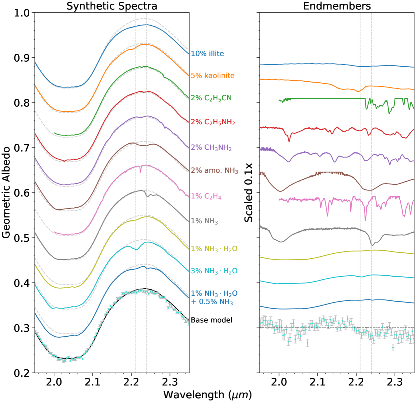
Figure 6: (Left panel): Synthetic spectra generated with a Hapke-Mie modeling program to investigate potential absorption features in the 2.2-$\mu$m region, compared to the UT201008 GNIRS spectrum of Miranda’s leading hemisphere (bottom, binned by 10 pixels). The synthetic spectra are described in Table 8. The left panel includes comparison spectra in which a small percentage of the 27.5-$\mu$m H₂O ice in the base model is replaced with an additional component of different composition, with a grain size of 10 µm. Vertical lines are placed at 2.21 and 2.24 µm. (Right panel): as the left panel, but using synthetic spectra of the corresponding pure (100%) ices at 10 $\mu$m grain size, scaled by a factor of 0.1. The observed GNIRS spectrum is divided by the base model.

Table 8: Synthetic spectra for Figure 6

Short name	Component 1	Component 2	Component 3	Component 4	$\chi_{\nu}^{2}$	Source
Base model	95.25% H2O 27.5$\mu m$	4.5% AC 5$\mu m$	0.25% H2O 0.3$\mu m$	$\cdots$	1.050	see caption
10% illite	85.25% H2O 27.5$\mu m$	4.5% AC 5$\mu m$	0.25% H2O 0.3$\mu m$	10% illite 10$\mu m$	2.762	Clark et al. (1990)
5% kaolinite	90.25% H2O 27.5$\mu m$	4.5% AC 5$\mu m$	0.25% H2O 0.3$\mu m$	5% kaolinite 10$\mu m$	1.202	Clark et al. (1990)
2% propionitrile	93.25% H2O 27.5$\mu m$	4.5% AC 5$\mu m$	0.25% H2O 0.3$\mu m$	2% C2H5CN 10$\mu m$	1.351	Moore et al. (2010)
2% ethylamine	93.25% H2O 27.5$\mu m$	4.5% AC 5$\mu m$	0.25% H2O 0.3$\mu m$	2% C2H5NH2 10$\mu m$	1.252	Hudson et al. (2022)
2% methylamine	93.25% H2O 27.5$\mu m$	4.5% AC 5$\mu m$	0.25% H2O 0.3$\mu m$	2% CH3NH2 10$\mu m$	1.236	Hudson et al. (2022)
2% amo. NH3	93.25% H2O 27.5$\mu m$	4.5% AC 5$\mu m$	0.25% H2O 0.3$\mu m$	2% amorph. NH3 10$\mu m$	0.938	Roser et al. (2021b)
1% ethylene	94.25% H2O 27.5$\mu m$	4.5% AC 5$\mu m$	0.25% H2O 0.3$\mu m$	1% C2H4 10$\mu m$	1.212	Hudson et al. (2014)
1% NH3	94.25% H2O 27.5$\mu m$	4.5% AC 5$\mu m$	0.25% H2O 0.3$\mu m$	1% cubic NH3 10$\mu m$	0.908	Hudson et al. (2022)
1% NH${}_{3}\cdot$H2O	94.25% (1%)NH${}_{3}\cdot$H2O 27.5$\mu m$	4.5% AC 5$\mu m$	0.25% H2O 0.3$\mu m$	$\cdots$	1.051	see caption
3% NH${}_{3}\cdot$H2O	94.25% (3%)NH${}_{3}\cdot$H2O 27.5$\mu m$	4.5% AC 5$\mu m$	0.25% H2O 0.3$\mu m$	$\cdots$	1.602	see caption
Mixed NH3	94.75% (1%)NH${}_{3}\cdot$H2O 27.5$\mu m$	4.5% AC 5$\mu m$	0.25% H2O 0.3$\mu m$	0.5% cubic NH3 10$\mu$m	0.939	see caption

Note. — The components of the synthetic Hapke-Mie spectra plotted in Figure 6, with their mixing ratios and grain sizes for each component. All spectra are intimate (particulate) mixtures. Components listed as ‘H₂O’ use optical constants of 80 K crystalline ice from Mastrapa et al. (2008), while the component listed as ‘AC’ is amorphous carbon, using the optical constants of sample BE1 from Rouleau & Martin (1991). Optical constants for other components are listed in the table. The NH₃-hydrate spectra replace the primary H₂O ice component with the optical constants of 1% and 3% by weight mixtures (respectively) of NH${}_{3}\cdot$H₂O. Reflectance spectra of these mixtures were originally measured by Brown et al. (1988), with optical constants derived by T. Roush (personal communication) and published in Cruikshank et al. (2005).

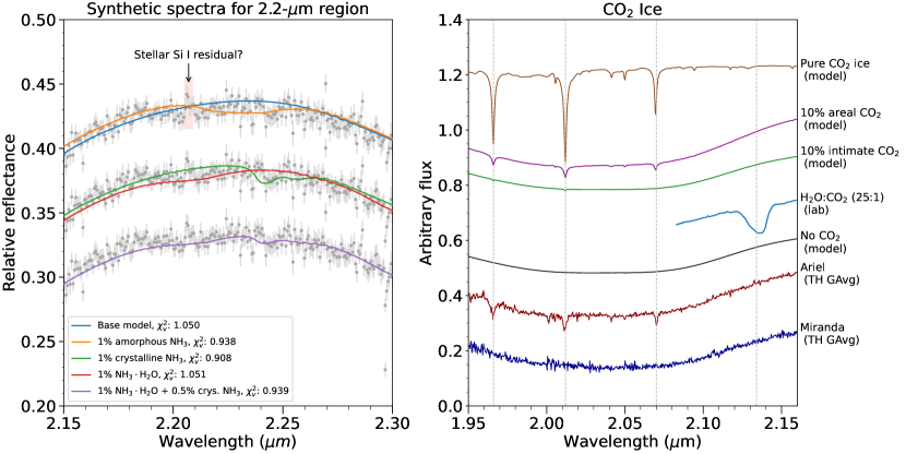
Figure 7: (Left panel): A close-up of the most promising NH₃-bearing synthetic models from Figure 6, compared to the UT201008 GNIRS spectrum of Miranda’s leading hemisphere. The synthetic spectra are described in Table 8. Small periodic variations are visible in the synthetic spectra due to resonances from the calculated Mie scattering solutions. (Right panel): A demonstration of the lack of CO₂ ice features on Miranda’s trailing hemisphere, compared to the trailing hemisphere of Ariel (Cartwright et al., 2022). We include several Hapke model spectra: pure CO₂ ice (10 $\mu$m grains), a base model (Table 8), the base model with 10% areally mixed CO₂ ice (27.5 $\mu$m grains), and the base model with 10% intimately mixed CO₂ ice (27.5 $\mu$m grains). We also include a laboratory spectrum of a H₂O:CO₂ ice molecular mixture (Bernstein et al., 2005), which displays a prominent 2.13-$\mu$m 2$\nu_{3}$ overtone band. Note that this forbidden overtone does not appear in pure CO₂ ice or the model spectra of H₂O:CO₂ ice intimate mixtures.

Synthetic Hapke-Mie spectra of intimate mixtures including some of the same materials as in Cartwright et al. (2023) are plotted in Figure 6 and tabulated in Table 8. We compared these synthetic spectra to a spectrum of Miranda’s leading hemisphere obtained with GNIRS (spectrum UT201008). This spectrum was chosen for being both high S/N and showing weak absorption in the 2.2-$\mu$m region. This absorption is composed of a shallow dip between 2.19 – 2.23 µm, along with a possible feature at 2.24 $\mu$m (Figure 7). We constructed a base model composed of two grain sizes of H₂O ice (27.5 $\mu$m and 0.3 µm), along with an amorphous carbon component to act as a dark, spectrally neutral absorber.

To demonstrate the lack of CO₂ ice absorption features, we calculated spectral models incorporating CO₂ ice and plotted them against observed spectra in Figure 7. Spectral models of pure or intimately-mixed CO₂ ice fail to reproduce the 2.13-$\mu$m 2$\nu_{3}$ overtone band seen in laboratory spectra of CO₂ ice in a molecular mixture with H₂O (Bernstein et al., 2005). A spectrum of Ariel’s trailing hemisphere (Cartwright et al., 2022) shows clear signatures of CO₂ ice, as previously discussed (§1.2). In comparison, the Miranda trailing hemisphere grand average spectrum shows no evidence of any absorption features resulting from CO₂ ice, either as separate deposits or trapped in the regolith.

To investigate species that could be contributing to absorption features in the 2.2-$\mu$m range, we constructed models in which we replaced small percentages of the H₂O ice component in the base model with other materials, including some of the same materials as in Cartwright et al. (2023) (Figure 6). From visual inspection, the complex absorption bands of propionitrile (C₂H₅CN), ethylamine (C₂H₅NH₂) and methylamine (CH₃NH₂) are somewhat difficult to interpret, but do not match the Miranda spectrum closely. Ethylamine and methylamine have band complexes between 1.65 – 1.80 $\mu$m which are also not apparent in our spectra. The 2.22-$\mu$m band of ethylene (C₂H₄) is too sharp compared to the broad absorptions of the Miranda spectra. The 2.2-$\mu$m bands of the aluminum-bearing phyllosilicates illite and kaolinite are subtle, but both of these minerals also have bands at 1.4 $\mu$m from bound water absorption. The wavelengths between 1.38 – 1.43 $\mu$m are hard to observe from Earth due to strong atmospheric H₂O absorption. Spectra with good telluric correction observed in dry conditions (such as the GNIRS spectra) do not show convincing evidence for the presence of the 1.4-$\mu$m band, but it is difficult to rule out either kaolinite or illite given the lower S/N in the region.

We also calculated $\chi_{\nu}^{2}$ values as a comparison between the observed spectrum and the constructed models, using the wavelengths between 2.15 – 2.29 $\mu$m (Table 8). The synthetic intimate mixture spectra we generated are not unique solutions, but are useful as general guidelines for interpretation of spectral features. Both cubic (crystalline) and amorphous NH₃ mixtures have significantly improved $\chi_{\nu}^{2}$ values compared to the base model, while a 1% mixture of NH${}_{3}\cdot$ H₂O fits the data equally as well as the base model ($\chi_{\nu}^{2}$ of 1.051 versus 1.050). Kaolinite, propionitrile, ethylene, ethylamine, methylamine, the 3% mixture of NH${}_{3}\cdot$ H₂O, and illite all have worse $\chi_{\nu}^{2}$ values than the base model.

While amorphous NH₃ ice has one of the most favorable $\chi_{\nu}^{2}$ values, it is unlikely that amorphous NH₃ could persist on Miranda’s surface, as it transitions to crystalline NH₃ when warmed to temperatures between 70 – 90 K (Moore et al., 2007). Voyager 2 measured a surface brightness temperature for Miranda of about 86 K (Hanel et al., 1986), and thermodynamical modeling predicts peak surface temperatures for the Uranian satellites around 90 K (Sori et al., 2017). Crystalline NH₃ ice produces a band at 2.24 µm, which is at longer wavelengths than the broad 2.2-$\mu$m feature in most of our spectra, but does correspond to the weak feature at 2.24 $\mu$m seen in this observed GNIRS spectrum (Figure 7). We also find a promising match between the spectrum in which the major H₂O ice component is replaced with a 1% mixture of NH₃-hydrates, which produces a shallow shoulder feature. However, the 3% NH₃-hydrates mixture produces a distinct 2.2-$\mu$m absorption band that is too strong compared to the weak absorption in the observed spectrum. We further investigated the possibility of NH₃ species by generating an additional model with both NH₃-hydrates and a small percentage of crystalline NH₃ ice. With the exception of the residual noise spike at 2.207 $\mu$m from incomplete solar line cancellation (§A), this model visually matches the weak absorption bands at 2.2 $\mu$m and 2.24 $\mu$m more closely. This ’mixed NH₃’ model has effectively the same $\chi_{\nu}^{2}$ value as the amorphous NH₃ model.

6 Discussion

Our band analysis procedures did not detect any evidence for the presence of crystalline CO₂ ice on Miranda’s surface, unlike its high abundance on the neighboring moon Ariel. Even in the high S/N spectra from GNIRS and the grand-average spectra from TripleSpec combining multiple nights of data, the three prominent CO₂ ice bands between 1.9 and 2.1 $\mu$m are not present (Figure 7). Additionally, we detected essentially no evidence for an absorption feature near 2.13 $\mu$m that might have hinted at the presence of CO₂ in a molecular mixture. In contrast, a subtle 2.2-$\mu$m band is exhibited by many of the Miranda spectra we analyzed.

6.1 CO₂ ice

The prevailing hypothesis for the origin of CO₂ ice on the other classical Uranian moons is a radiolytic production mechanism (§1.2). This hypothesis states that the observed CO₂ is produced in situ via irradiation of surface carbon compounds and H₂O ice, which recombine to form CO₂ and other products. Sublimation, sputtering, and other processes cause the CO₂ molecules to ‘hop’ in suborbital trajectories across the surface until they either escape or land in a cold trap. Because of the large obliquity of the Uranian system, the parts of the surface that receive the lowest amount of time-averaged sunlight over the Uranian year are at low latitudes. Crystalline CO₂ ice is bright and highly reflective, decreasing absorbed solar energy and likely reducing sublimation of CO₂ molecules from cold traps once they have been established. Theoretically, the trailing hemispheres would accumulate more CO₂ ice because the magnetosphere of Uranus rotates faster than the moons orbit, and might preferentially irradiate their trailing hemispheres and produce CO₂ molecules, thereby explaining the observed distribution of CO₂ on Ariel, Umbriel, Titania, and Oberon (Grundy et al., 2003, 2006; Cartwright et al., 2015, 2022). However, the exact nature of interactions between Uranus’ offset and tilted magnetosphere and the surfaces of the moons are still poorly understood (e.g. Kollmann et al., 2020).

In contrast, this lack of CO₂ ice on Miranda, where radiolytic production of CO₂ molecules should be possible, could result from its small mass and lower efficiency of retaining volatiles like CO₂. Previous works have extensively discussed potential mechanisms for production and destruction of CO₂ on the Uranian satellites, such as photolysis or sputtering by charged particles (Grundy et al., 2006; Cartwright et al., 2015; Sori et al., 2017; Steckloff et al., 2022). Most importantly, a large fraction of the expected thermal velocity distribution of sputtered or sublimated CO₂ molecules is greater than the escape velocity of Miranda (193 m s^-1). Sori et al. (2017) found that approximately half of all CO₂ molecules sublimated on Miranda would escape before completing a single suborbital ‘hop’. Steckloff et al. (2022) found a similar result, adding that the time required for these CO₂ molecules to migrate to the antipode of their initial production site on Miranda ($\sim$14 hours) is more than an order of magnitude longer than their expected residence time in the exosphere before escape (approximately one hour). Other processes that could destroy CO₂ ice are effectively irrelevant on Miranda, given the rate at which any produced or otherwise mobilized CO₂ molecules would be lost. Miranda cannot retain significant CO₂ ice deposits with such a large loss fraction. It is therefore not surprising that we do not observe any CO₂ ice deposits on Miranda.

However, given the assumption of ongoing radiolytic production, it is still possible that CO₂ is present in Miranda’s regolith, perhaps as molecules mixed with H₂O ice. This motivated our search for a 2.13-$\mu$m absorption band, attributed to the forbidden $2\nu_{3}$ first overtone of the strong 4.27-$\mu$m $\nu_{3}$ asymmetric stretch band of CO₂. This forbidden feature is extremely weak in spectra of pure CO₂ ice, but becomes apparent when CO₂ is in a molecular mixture with other ices, including H₂O and CH₃OH (Bernstein et al., 2005). This overtone can vary significantly in its depth and shape in laboratory spectra. In many of our high S/N spectra, visual inspection suggested a weak feature centered at slightly shorter wavelengths ($\sim$2.130 µm), reminiscent of a weak 2.13-$\mu$m band detected on Ariel using SpeX and TripleSpec data (Cartwright et al., 2022), also centered at $\sim$2.130 $\mu$m and spanning 2.123 – 2.137 µm. If a molecular mixture including CO₂ ice is responsible for this band on Ariel, then it could also be responsible for a similar band on Miranda. However, our band analyses did not find convincing evidence for the 2.13-$\mu$m band on Miranda. If CO₂ is being produced on Miranda, it is not being trapped in the regolith in sufficient quantities to manifest the 2.13-$\mu$m band at a strength detectable in our spectra.

6.2 NH₃-bearing species

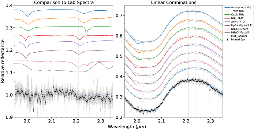
Figure 8: (Left panel): The UT201008 GNIRS spectrum of Miranda’s leading hemisphere (gray errorbars native resolution, black errorbars binned by 5 pixels), compared to several laboratory-measured absorbance spectra of NH-bearing species (digitized from Figures 6 and 14 of Moore et al. (2007)). The laboratory spectra are arbitrarily scaled and offset. We also include a reflectance spectrum of NH₄Cl at 90 K from Fastelli et al. (2022). (Right panel): Arbitrarily scaled linear combinations of the lab spectra with our synthetic base model for qualitative comparison of band shapes and locations. Vertical lines are placed at 2.21 and 2.24 µm.

Table 9: $\chi_{\nu}^{2}$ values of different comparison spectra

Short name	Figure	Spectrum type	$\chi_{\nu}^{2}$
Base model	6,7,8,9	Hapke-Mie	1.050
10% illite	6	Hapke-Mie	2.762
5% kaolinite	6	Hapke-Mie	1.202
2% propionitrile	6	Hapke-Mie	1.351
2% ethylamine	6	Hapke-Mie	1.252
2% methylamine	6	Hapke-Mie	1.236
2% amorphous NH3	6,7	Hapke-Mie	0.938
1% ethylene	6	Hapke-Mie	1.212
1% NH3	6,7	Hapke-Mie	0.908
1% NH${}_{3}\cdot$H2O	6,7	Hapke-Mie	1.051
3% NH${}_{3}\cdot$H2O	6	Hapke-Mie	1.602
Mixed NH3	6,7	Hapke-Mie	0.939
Amorphous NH3	8	base + lab absorbance	0.824
Transition-phase NH3	8	base + lab absorbance	0.884
Cubic NH3	8	base + lab absorbance	1.065
NH${}_{3}\cdot$H2O	8	base + lab absorbance	1.014
2NH${}_{3}\cdot$H2O	8	base + lab absorbance	0.928
NH3+H2O ($\sim$5:1)	8	base + lab absorbance	0.959
Moore NH4Cl	8	base + lab absorbance	0.952
Fastelli NH4Cl	8,9	base + lab reflectance	73.222

Note. — Comparison of $\chi_{\nu}^{2}$ values of our constructed comparison spectra in various figures (measured between the models and unbinned data between 2.15–2.29 µm). For details on the Hapke-Mie models, see Table 8. The linear combinations of the Hapke-Mie base model and the laboratory absorbance spectra are arbitrarily scaled and are not quantitatively comparable to the other Hapke-Mie synthetic spectra.

In Figure 8, we utilized the laboratory absorption spectra of Moore et al. (2007) to investigate the potential contributions of NH₃ species. Moore et al. measured the absorption spectra of multiple phases of pure NH₃ ice, several NH₃-H₂O mixtures, two phases of NH₃-hydrates, and NH₄Cl (from Moore et al. (2003)). We also constructed qualitative linear mixtures using these absorption spectra to qualitatively compare band shapes and locations (right panel of Figure 8). These are not physically accurate spectral models, but provide a general idea of how low-level absorption from these features might appear. Quantitative spectral modeling would require the optical constants of these species to be measured, and optical constants have only been published for amorphous NH₃ ice, crystalline NH₃ ice, and an NH₃-hydrate of uncertain stoichiometry (Figures 6,7).

Pure NH₃ ices of any phase produce bands at longer wavelengths than the broad 2.2-$\mu$m band in the Miranda spectrum, but could contribute to shallow absorptions at 2.24 µm. The NH₃-H₂O hydrates and NH₃-H₂O mixture produce a broad band centered between $\sim$2.21 – 2.22 µm. Both 2NH${}_{3}\cdot$H₂O and the absorbance spectrum of NH₄Cl produces a double-band structure with a 2.21-$\mu$m and 2.24-$\mu$m band. From visual inspection, the NH₃-hydrates and NH₃-H₂O mixtures provide acceptable matches, but NH₄Cl (Moore) seems to match the shape and position of the weak 2.2-$\mu$m bands in the Miranda spectrum best. When we compare the calculated $\chi_{\nu}^{2}$ values of these linear combinations to the spectrum (Table 9), all but the cubic NH₃ mixture have improved $\chi_{\nu}^{2}$ values over the base model ($\chi_{\nu}^{2}=$1.050). As with the synthetic Hapke-Mie spectra, amorphous NH₃ ice has the best $\chi_{\nu}^{2}$, but amorphous and transition-phase NH₃ ice do not produce band shapes that visually match the Miranda spectrum, and their presence on Miranda is unlikely (§5). The cubic NH₃ ice alone produces a visual fit to the 2.24-$\mu$m band, but not the band between 2.18 – 2.23 µm. Conversely, the 2.18 – 2.23-$\mu$m band is well fit by the NH₃-hydrates and NH₃-H₂O mixtures. The 2NH${}_{3}\cdot$H₂O and Moore NH₄Cl spectra produce bands at both 2.18 – 2.23 $\mu$m and 2.24 µm, more consistent with the observed Miranda spectrum. When excluding the amorphous and transition-phase NH₃ ices, then 2NH${}_{3}\cdot$H₂O, the Moore NH₄Cl spectrum, and the NH₃-H₂O mixture have the best $\chi_{\nu}^{2}$.

However, all of the Moore et al. lab spectra of NH₃-bearing species show the 2.0-$\mu$m band of NH₃ ice, which is not visible in our spectra. This 2.0-$\mu$m absorption band is rarely detected on icy bodies. Even in the case of Charon, where the 2.21-$\mu$m band is obvious, the presence of a complementary 2.0-$\mu$m band is uncertain (Cook et al., 2018, 2023). The 2.0-$\mu$m band is difficult to detect from ground-based spectra, as it lies in the spectral noise from a deep telluric CO₂ band, and even in spectra from New Horizons, the 2.0-$\mu$m band is not as strong as would be expected from laboratory spectra (Cook et al., 2018; Protopapa et al., 2021). The strong H₂O absorption band at 2.0 $\mu$m further means that light penetrates much shallower into the regolith ($\sim$ 0.1 mm at 2.0 µm) than it does at 2.24 $\mu$m ($\sim$ 1.6 mm), where H₂O only contributes weak absorption and the optical path length is therefore longer (Cartwright et al., 2023). NH₃-bearing species could be present in the subsurface, where they only appear in absorption in regions of the spectrum where the optical path length is long enough to reach them, contributing to the difficulty of detecting the NH₃ 2.0-$\mu$m absorption feature, or an ammonium salt such as NH₄Cl that lacks a 2.0-$\mu$m band could be responsible (next section). We also note that these qualitative linear combinations do not incorporate effects like multiple scattering that would make a difference in the strength of the 2.0-$\mu$m band. This is demonstrated by the difference in the strength of the 2.0-$\mu$m band in the Hapke-Mie synthetic spectra with NH₃ ice (Figure 6), in which the band is much less prominent than in our linear combinations.

The ‘survivability’ of NH₃-bearing species is also an open question. As discussed previously, NH₃-bearing species exposed at the surface of icy bodies are expected to be dissociated by particle irradiation (such as cosmic rays) on geologically short timescales. Miranda is subject to additional proton and electron bombardment from charged particles trapped in Uranus’s magnetosphere, and Moore et al. (2007) estimate timescales for destruction of NH₃ ice at Miranda’s surface as short as $\sim 10^{6}$ years. However, dissociated NH₃ does not simply disappear. The radiation products can readily recombine into similar forms, such as NH${}_{4}^{+}$ ions, which can react with other compounds to form NH₄-bearing salts. Protopapa et al. (2021) provides a lengthy review of the mechanisms that could destroy NH₃ on Charon. While the radiation environment on Miranda is more hostile to NH₃, NH₄-bearing species still possess a 2.2-$\mu$m band, and NH₄-bearing salts may be more resistant to destruction by irradiation.

6.3 NH₄-bearing species and other refractory compounds

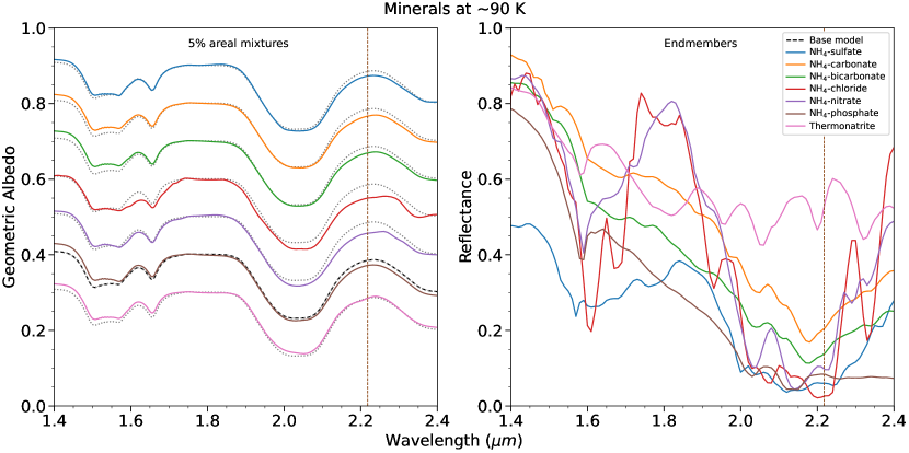
Figure 9: (Left panel): Our base model of Miranda’s spectrum compared to 5% areal mixtures of NH₄-bearing minerals and thermonatrite. The mixture spectra were normalized to match the base model at 1.754 µm, then offset in increments of 0.1. The vertical line marks the mean wavelength of our 2.2-$\mu$m band measurements at 2.218 µm. (Right panel): NH₄-bearing mineral reflectance spectra measured at 90 K from Fastelli et al. (2022) and thermonatrite measured at 93 K from De Angelis et al. (2019).

Ammonium salts such as NH₄Cl have been proposed as a candidate species partially or wholly responsible for the 2.2-$\mu$m absorption band on Charon and on other bodies in the Pluto system (Moore et al., 2007; Cook et al., 2007, 2018, 2023). NH₄Cl has also been reported in the bright emplaced material in Occator Crater on Ceres (Raponi et al., 2019). Other NH₄-bearing species, such as ammonium carbonate ((NH₄)₂CO₃) or ammonium bicarbonate (NH₄HCO₃), have also been implicated in the presence of a 2.2-$\mu$m absorption (de Sanctis et al., 2016; Cartwright et al., 2020b). The NH${}_{4}^{+}$ ion is a byproduct of irradiation of NH₃-H₂O mixtures (Moore et al., 2007), and given other suitable species to react with, it could form NH₄-bearing salts. In Figure 9, we plot reflectance spectra of NH₄-bearing species measured at 90 K from Fastelli et al. (2022), and constructed linear (areal) mixture models of our synthetic base model spectrum, plus a 5% abundance of various species. The absorption bands of most of these species, with the possible exception of NH₄Cl, are at too short wavelengths to account for the 2.2-$\mu$m band we see on Miranda, but could contribute to low-level absorption between 2.18 – 2.25 µm. As seen in the figure, their broad absorption features tend to simply depress the 2.2-$\mu$m continuum of H₂O ice relative to the 1.8-$\mu$m continuum. Miranda’s spectrum exhibits the same characteristic, but the broad nature of these NH₄ absorptions observed in reflectance generally limits the ability to identify them, as a depressed 2.2-$\mu$m continuum could also result from sub-micron H₂O ice grains (§3.3) or any other compound with a strong blue slope between 1.8 and 2.2 µm.

However, linear (areal) mixture modeling comes with additional caveats. Linear mixture modeling does not incorporate the nonlinear effects of multiple scattering (important for bright icy surfaces) or other factors in the reflectance of a particular component, such as grain size. These effects are treated in intimate mixture models, but an intimate mixture model requires the optical constants of the material to be measured, and no optical constants for these NH₄-bearing species have been published in the scientific literature. Furthermore, direct comparison demonstrates that the reflectance spectrum of a pure compound is distinctly different from the absorption spectrum; compare and contrast the absorbance spectra and reflectance spectra of NH₄Cl in Figure 8. Although the spectra are arbitrarily scaled, the difference in depths and shapes of the absorption bands are clearly apparent. The Fastelli et al. sample studied in reflectance is much thicker ($\sim$ mm) than the Moore et al. sample studied in absorbance (tens of microns), which makes weaker features easier to detect, but produces saturation and blending of the stronger absorption features. The relative band strengths are different between the Moore and Fastelli NH₄Cl spectra: the weak absorptions between 2.0 and 2.2 $\mu$m in the Moore spectrum are heavily blended in the Fastelli spectrum, and the stronger absorptions at 2.21 and 2.24-$\mu$m are effectively saturated. The Fastelli spectrum also shows a clear band at 2.34-$\mu$m that is shallow in the Moore spectrum and absent in the Miranda spectra. Finally, the spectral resolution of the Fastelli spectra are generally inadequate compared to our Miranda spectra and the Moore spectrum.

While our spectra of Miranda were also observed in reflectance, an intimate mixture of small percentages of NH₄Cl or another NH₄-bearing species in H₂O ice could produce a spectral signature more similar to the Moore et al. absorption spectrum. We also note that unlike the rest of the NH₃-bearing species in Figure 8, NH₄Cl lacks a strong 2.0-$\mu$m band, consistent with the lack of the 2.0-$\mu$m band in our spectra of Miranda. Confident quantitative estimates are difficult given the weak 2.2-$\mu$m absorption, the limited nature of the available laboratory data, and the lack of optical constants for candidate constituents. We suggest that an NH₄-bearing species, perhaps NH₄Cl, may be partially or wholly responsible for the 2.2-$\mu$m band, although NH₃-bearing species could contribute to absorption in this range.

The potential sources (and potential destruction) of NH₄Cl on Charon is discussed thoroughly in Cook et al. (2023). Many of these arguments are also applicable at some level to the Uranian satellites, including Miranda. Chlorine could be delivered to the surface via impacts, or perhaps an endogenic process like cryovolcanism emplaced NaCl-bearing or NH₄Cl-bearing brines and/or NH₃-rich liquids onto the surface. Some form of this process, likely impact-induced, appears to have occurred at Ceres in Occator Crater (Raponi et al., 2019; De Sanctis et al., 2020). Furthermore, carbonaceous material and H₂O are readily available at Miranda’s surface and particle irradiation is present to dissociate them. In addition to the previously-discussed CO₂, if Miranda’s surface was supplied with NH₃- or NH₄-bearing species, NH₄-bearing carbonates could be a common byproduct.

With previous results on Umbriel in mind (Cartwright et al., 2023), we also generated a synthetic intimate mixture model incorporating the aluminum-bearing phyllosilicates illite and kaolinite (Figure 6), and an areal mixture model incorporating the hydrated Na-bearing carbonate thermonatrite (Figure 9). Thermonatrite’s 2.2-$\mu$m band is centered at shorter wavelengths than our mean band center (2.201 versus 2.218 µm), but could be contributing to wider low-level absorption between 2.18 – 2.25 $\mu$m (Figure 2). Kaolinite has a blue slope at wavelengths longer than 1.8 $\mu$m and a double-band absorption at 2.16 and 2.206 $\mu$m that could produce a similar shoulder feature, but as discussed in §5, the only other strong indicator of phyllosilicates in the near-IR ($<$2.5 µm) is generally the 1.4-$\mu$m band, which is difficult to observe from Earth due to telluric absorption.

7 Conclusions

We conclude that there is no crystalline CO₂ ice concentrated in discrete deposits on Miranda’s surface, consistent with the explanation that Miranda’s weak surface gravity allows CO₂ molecules to efficiently escape before being cold trapped. Similarly, we detected no convincing evidence of a 2.13-$\mu$m band that could be associated with a molecular mixture of CO₂ in H₂O or CH₃OH ice.

In contrast, we detected a 2.2-$\mu$m band at $>2\sigma$ significance in several of our spectra. We do not see evidence for longitudinal trends or hemispherical asymmetries in the distribution of the 2.2-$\mu$m band. We compared a high S/N GNIRS spectrum of the leading hemisphere to synthetic spectra and laboratory spectra of several candidate species, including NH-bearing species, nitrogen-bearing organics, and phyllosilicates. We found that the 2.2-$\mu$m feature can be best explained by either a combination of NH₃-bearing species (e.g. NH₃-hydrates and NH₃ ice) or by an NH₄-bearing salt like NH₄Cl, but NH₄-carbonates or certain phyllosilicates like kaolinite could contribute to broad and shallow absorption between 2.18 – 2.25 µm.

However, the study of NH₃-bearing and NH₄-bearing species is substantially limited by the available laboratory data. Optical constants of candidate species are few and far between, and reflectance data are often acquired at room temperature and with insufficient spectral resolution to properly capture the blended spectral bands that change position and strength with temperature and composition. Common minerals often show fine structure in absorption bands that are not detected in low resolution reflectance spectra (Clark et al., 1990). Further laboratory work to determine optical constants of NH₃-hydrates, NH₃-H₂O mixtures, and NH₄-bearing salts at high resolution and cryogenic temperatures in the near- to mid-IR should be a high priority for the icy satellites community (Dalton, 2010). The results of such laboratory work (spectra and optical constants) must be made publicly downloadable in a data repository for current and future scientists (Roser et al., 2021a).

Future investigations of CO₂ ice and NH₃-bearing species on Miranda could be carried out with JWST, as the excellent sensitivity of a 6.5-meter IR-optimized space telescope is hard to match even with larger ground-based telescopes. JWST has the ability to investigate the 4.27-$\mu$m CO₂ ice $\nu_{3}$ fundamental absorption band, which lies within a wavelength range in which the Earth’s atmosphere is completely opaque. This fundamental absorption band is a factor of $\sim$10³ stronger than the 2-$\mu$m overtone bands, and the lack of the 2.13-$\mu$m band suggests that JWST observations of the 4.27-$\mu$m band would be more suitable for further constraining CO₂ ice on Miranda and the other Uranian moons. NH₃-bearing species would be detectable by JWST with the NH₃ $\nu_{3}$ fundamental band (2.96-µm) and the hydrated nitrogen (OH-N) features (3.05-$\mu$m and 3.1 – 3.2 µm) overprinted on the wide 3.0-$\mu$m H₂O ice band. These bands are far stronger than the weak overtone bands in the near-IR shortward of 2.5 µm, and different NH-bearing compounds and hydration states are much easier to distinguish from each other at longer wavelengths (Moore et al., 2007). Similarly, NH₄-bearing minerals can be detected through features between 3.0 – 3.5 $\mu$m (Bishop et al., 2002; Berg et al., 2016).

Spatially resolved spectroscopy of ices on Miranda and the other Uranian satellites would be most effectively carried out by a Uranus orbiter equipped with a NIR imaging spectrometer, analogous to VIMS on Cassini or MISE on the upcoming Europa Clipper mission. The Uranus Orbiter and Probe was the highest priority new Flagship mission recommended by the 2023-2032 Decadal Survey. Such a mission would be able to revolutionize our knowledge of the entire Uranian system, including the icy satellites, and could investigate spatial and spectral variations in surface composition in far more detail than could ever be achieved from Earth.

Appendix A Spectral contamination

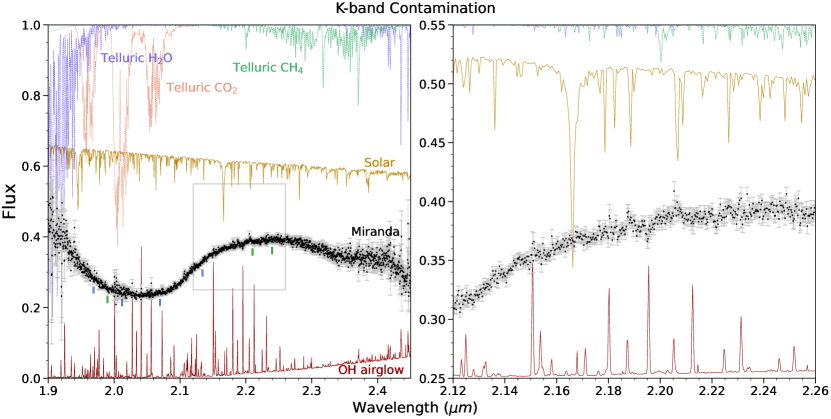
Figure 10: (Left panel): Sources of spectral contamination in K-band. The atmospheric transmission curves for telluric species are plotted as the fraction of light transmitted and have correct scaling relative to each other. The solar spectrum has been divided by a 5777 K blackbody spectrum. The plotted Miranda spectrum is a grand average of all TripleSpec spectra. The scaling on the solar, airglow, and Miranda spectrum are arbitrary for visualization purposes. The wavelengths of the absorption features of interest in this work are annotated below the Miranda spectrum: the CO₂ ice triplet and the 2.13-$\mu$m band are marked in blue, and features associated with NH₃-bearing species are marked in green. (Right panel): Inset zoom for the box marked in the left panel. Note the ’spike’ residuals in the Miranda spectrum that closely match OH and solar lines.

Potential absorption features in the spectrum of Miranda in K-band are also subject to low-level contamination from various sources (Figure 10). Absorption from gases in Earth’s atmosphere (telluric absorption) is a significant concern for ground-based observations in the near-infrared. Atmospheric H₂O vapor is often the most difficult species to correct for, as it has a multitude of strong, narrow absorption lines, and precipitable water vapor along the line of sight can vary locally on short spatial and temporal scales. However, absorption from atmospheric H₂O is not a major concern between 2.00 – 2.40 µm, which encompasses almost all of the absorption features of interest in this work.

Telluric CO₂ has three strong overtone bands which are the major source of atmospheric absorption between 1.95 – 2.10 µm. Unlike H₂O absorption, which varies strongly due to local weather conditions, CO₂ is well-mixed in the Earth’s atmosphere and variations in absorption strength are largely based on optical path length through the atmosphere (airmass). However, fine structure in the deepest parts of the CO₂ overtone bands are partially resolved in our highest-resolution data (R$\sim$3500), and telluric correction procedures often leave high-frequency residual noise in these regions. This is visible in many of the Miranda spectra as an increased scatter in the data points between 2.00 – 2.02 µm, and to a lesser extent between 1.95 – 1.97 and 2.05 – 2.07 µm. These wavelengths ranges overlap the narrow CO₂ ice bands, but this should not prevent the detection of CO₂ ice given the high S/N of this dataset.

The 2.2-$\mu$m region experiences weak absorption from narrow atmospheric CH₄ bands, with a somewhat stronger feature at 2.200-µm. However, like CO₂, telluric CH₄ is generally well-mixed in the Earth’s atmosphere. We find that the usual telluric standard procedures are effective at correcting absorption features from atmospheric CH₄, as evidenced by the lack of residuals from the other CH₄ absorption lines in K-band, so we do not expect Miranda’s 2.2-$\mu$m feature to be contaminated to a substantial degree by atmospheric CH₄. Atmospheric CO₂ and H₂O do not have significant absorption features between 2.10 – 2.35 µm.

OH airglow emission lines are generally well-corrected in our spectra, but stacking many spectra can leave small positive or negative residual features and increased error estimates on certain data points, such as at 2.041, 2.150, and 2.195 µm. The upwards slope of the continuum in the plotted OH spectrum at longer wavelengths ($>$2.1 µm) is blackbody radiation from the telescope and atmosphere. This slope is subtracted from the science data during data reduction procedures and does not factor into the final spectra.

We also note that there are mismatches in the strength of stellar absorption features between the G-type telluric standard stars and the reflected solar spectrum. When dividing the observed spectra of the object by the standard star, these mismatches appear as narrow residual ’spikes’ or ’dips’ in the final spectrum. This includes the inconvenient presence of a residual spike at 2.207 µm, which appears to be due to a mismatch in the strength of a Si I metal line (see Figure 7). This identification is supported by other small, but noticeable positive residuals from other Si I lines in K-band at 2.093, 2.135, and 2.188 $\mu$m (Mohler et al., 1953). Larger mismatches are also sometimes apparent in the strength of the H I Brackett $\gamma$ line at 2.166 µm, and any apparent absorption features in the range 2.155 – 2.175 $\mu$m should be treated with suspicion. In general, any narrow residual features in the high-resolution Miranda spectra appear to be either due to OH airglow lines or from mismatches in solar/stellar spectra.

Finally, we note that scattered light from the disk of Uranus is a major source of contamination in spectra of Miranda at wavelengths shorter than $\sim$1.7 µm. However, Uranus is very faint in K-band due to absorption by CH₄ and the H₂ pressure-induced dipole (Fink & Larson, 1979; Baines et al., 1998), which includes the wavelength ranges and absorption features of interest in this work. The contamination of the Miranda spectra by the spectrum of Uranus is therefore negligible for the purposes of this study.

References

- Afanasiev et al. (2014) Afanasiev, V. L., Rosenbush, V. K., & Kiselev, N. N. 2014, Astrophysical Bulletin, 69, 211, doi: 10.1134/S1990341314020096
- Astropy Collaboration et al. (2013) Astropy Collaboration, Robitaille, T. P., Tollerud, E. J., et al. 2013, A&A, 558, A33, doi: 10.1051/0004-6361/201322068
- Baines et al. (1998) Baines, K. H., Yanamandra-Fisher, P. A., Lebofsky, L. A., et al. 1998, Icarus, 132, 266, doi: 10.1006/icar.1998.5894
- Barkume et al. (2006) Barkume, K. M., Brown, M. E., & Schaller, E. L. 2006, ApJ, 640, L87, doi: 10.1086/503159
- Bauer et al. (2002) Bauer, J. M., Roush, T. L., Geballe, T. R., et al. 2002, Icarus, 158, 178, doi: 10.1006/icar.2002.6876
- Beddingfield et al. (2015) Beddingfield, C. B., Burr, D. M., & Emery, J. P. 2015, Icarus, 247, 35, doi: 10.1016/j.icarus.2014.09.048
- Beddingfield & Cartwright (2020) Beddingfield, C. B., & Cartwright, R. J. 2020, Icarus, 343, 113687, doi: 10.1016/j.icarus.2020.113687
- Beddingfield et al. (2022) Beddingfield, C. B., Leonard, E., Cartwright, R. J., Elder, C., & Nordheim, T. A. 2022, \psj, 3, 174, doi: 10.3847/PSJ/ac7be5
- Berg et al. (2016) Berg, B. L., Cloutis, E. A., Beck, P., et al. 2016, Icarus, 265, 218, doi: 10.1016/j.icarus.2015.10.028
- Bernstein et al. (2005) Bernstein, M. P., Cruikshank, D. P., & Sandford, S. A. 2005, Icarus, 179, 527, doi: 10.1016/j.icarus.2005.07.009
- Bishop et al. (2002) Bishop, J. L., Banin, A., Mancinelli, R. L., & Klovstad, M. R. 2002, Planet. Space Sci., 50, 11, doi: 10.1016/S0032-0633(01)00077-0
- Brown & Calvin (2000) Brown, M. E., & Calvin, W. M. 2000, Science, 287, 107, doi: 10.1126/science.287.5450.107
- Brown & Clark (1984) Brown, R. H., & Clark, R. N. 1984, Icarus, 58, 288, doi: 10.1016/0019-1035(84)90045-9
- Brown & Cruikshank (1983) Brown, R. H., & Cruikshank, D. P. 1983, Icarus, 55, 83, doi: 10.1016/0019-1035(83)90052-0
- Brown et al. (1988) Brown, R. H., Cruikshank, D. P., Tokunaga, A. T., Smith, R. G., & Clark, R. N. 1988, Icarus, 74, 262, doi: 10.1016/0019-1035(88)90041-3
- Carnall (2017) Carnall, A. C. 2017, arXiv e-prints, arXiv:1705.05165. https://arxiv.org/abs/1705.05165
- Carry et al. (2011) Carry, B., Hestroffer, D., DeMeo, F. E., et al. 2011, A&A, 534, A115, doi: 10.1051/0004-6361/201117486
- Cartwright et al. (2023) Cartwright, R. J., DeColibus, R. A., Castillo-Rogez, J. C., et al. 2023, \psj, 4, 28, doi: 10.3847/PSJ/acbc1f
- Cartwright et al. (2020a) Cartwright, R. J., Emery, J. P., Grundy, W. M., et al. 2020a, Icarus, 338, 113513, doi: 10.1016/j.icarus.2019.113513
- Cartwright et al. (2018) Cartwright, R. J., Emery, J. P., Pinilla-Alonso, N., et al. 2018, Icarus, 314, 210, doi: 10.1016/j.icarus.2018.06.004
- Cartwright et al. (2015) Cartwright, R. J., Emery, J. P., Rivkin, A. S., Trilling, D. E., & Pinilla-Alonso, N. 2015, Icarus, 257, 428, doi: 10.1016/j.icarus.2015.05.020
- Cartwright et al. (2020b) Cartwright, R. J., Beddingfield, C. B., Nordheim, T. A., et al. 2020b, ApJ, 898, L22, doi: 10.3847/2041-8213/aba27f
- Cartwright et al. (2022) Cartwright, R. J., Nordheim, T. A., DeColibus, R. A., et al. 2022, \psj, 3, 8, doi: 10.3847/PSJ/ac3d30
- Castillo-Rogez et al. (2023) Castillo-Rogez, J., Weiss, B., Beddingfield, C., et al. 2023, Journal of Geophysical Research (Planets), 128, e2022JE007432, doi: 10.1029/2022JE007432
- Clark et al. (1990) Clark, R. N., King, T. V. V., Klejwa, M., Swayze, G. A., & Vergo, N. 1990, J. Geophys. Res., 95, 12653, doi: 10.1029/JB095iB08p12653
- Clark et al. (2012) Clark, R. N., Cruikshank, D. P., Jaumann, R., et al. 2012, Icarus, 218, 831, doi: 10.1016/j.icarus.2012.01.008
- Cook et al. (2007) Cook, J. C., Desch, S. J., Roush, T. L., Trujillo, C. A., & Geballe, T. R. 2007, ApJ, 663, 1406, doi: 10.1086/518222
- Cook et al. (2018) Cook, J. C., Ore, C. M. D., Protopapa, S., et al. 2018, Icarus, 315, 30, doi: 10.1016/j.icarus.2018.05.024
- Cook et al. (2023) Cook, J. C., Protopapa, S., Dalle Ore, C. M., et al. 2023, Icarus, 389, 115242, doi: 10.1016/j.icarus.2022.115242
- Cruikshank et al. (2005) Cruikshank, D. P., Owen, T. C., Dalle Ore, C., et al. 2005, Icarus, 175, 268, doi: 10.1016/j.icarus.2004.09.003
- Cruikshank et al. (2019) Cruikshank, D. P., Umurhan, O. M., Beyer, R. A., et al. 2019, Icarus, 330, 155, doi: 10.1016/j.icarus.2019.04.023
- Cushing et al. (2004) Cushing, M. C., Vacca, W. D., & Rayner, J. T. 2004, PASP, 116, 362, doi: 10.1086/382907
- Dalle Ore et al. (2018) Dalle Ore, C. M., Protopapa, S., Cook, J. C., et al. 2018, Icarus, 300, 21, doi: 10.1016/j.icarus.2017.08.026
- Dalle Ore et al. (2019) Dalle Ore, C. M., Cruikshank, D. P., Protopapa, S., et al. 2019, Science Advances, 5, eaav5731, doi: 10.1126/sciadv.aav5731
- Dalton (2010) Dalton, J. B. 2010, Space Sci. Rev., 153, 219, doi: 10.1007/s11214-010-9658-7
- De Angelis et al. (2019) De Angelis, S., Carli, C., Tosi, F., et al. 2019, Icarus, 317, 388, doi: 10.1016/j.icarus.2018.08.012
- de Sanctis et al. (2016) de Sanctis, M. C., Raponi, A., Ammannito, E., et al. 2016, Nature, 536, 54, doi: 10.1038/nature18290
- De Sanctis et al. (2020) De Sanctis, M. C., Ammannito, E., Raponi, A., et al. 2020, Nature Astronomy, 4, 786, doi: 10.1038/s41550-020-1138-8
- DeColibus et al. (2022) DeColibus, R., Chanover, N., & Cartwright, R. 2022, \psj, 3, 119, doi: https://doi.org/10.3847/PSJ/ac694e
- DeMeo et al. (2015) DeMeo, F. E., Dumas, C., Cook, J. C., et al. 2015, Icarus, 246, 213, doi: 10.1016/j.icarus.2014.04.010
- Dumas et al. (2001) Dumas, C., Terrile, R. J., Brown, R. H., Schneider, G., & Smith, B. A. 2001, AJ, 121, 1163, doi: 10.1086/318747
- Emery et al. (2005) Emery, J. P., Burr, D. M., Cruikshank, D. P., Brown, R. H., & Dalton, J. B. 2005, A&A, 435, 353, doi: 10.1051/0004-6361:20042482
- Fastelli et al. (2022) Fastelli, M., Comodi, P., Schmitt, B., et al. 2022, Icarus, 382, 115055, doi: 10.1016/j.icarus.2022.115055
- Fink & Larson (1979) Fink, U., & Larson, H. P. 1979, ApJ, 233, 1021, doi: 10.1086/157466
- Gourgeot et al. (2014) Gourgeot, F., Dumas, C., Merlin, F., Vernazza, P., & Alvarez-Candal, A. 2014, A&A, 562, A46, doi: 10.1051/0004-6361/201321988
- Greenberg et al. (1991) Greenberg, R., Croft, S. K., Janes, D. M., et al. 1991, in Uranus, ed. J. T. Bergstralh, E. D. Miner, & M. S. Matthews (University of Arizona Press), 693–735
- Grundy et al. (1999) Grundy, W. M., Buie, M. W., Stansberry, J. A., Spencer, J. R., & Schmitt, B. 1999, Icarus, 142, 536, doi: 10.1006/icar.1999.6216
- Grundy et al. (2006) Grundy, W. M., Young, L. A., Spencer, J. R., et al. 2006, Icarus, 184, 543, doi: 10.1016/j.icarus.2006.04.016
- Grundy et al. (2003) Grundy, W. M., Young, L. A., & Young, E. F. 2003, Icarus, 162, 222, doi: 10.1016/S0019-1035(02)00075-1
- Grundy et al. (2016) Grundy, W. M., Binzel, R. P., Buratti, B. J., et al. 2016, Science, 351, aad9189, doi: 10.1126/science.aad9189
- Hammond & Barr (2014) Hammond, N. P., & Barr, A. C. 2014, Geology, 42, 931, doi: 10.1130/G36124.1
- Hanel et al. (1986) Hanel, R., Conrath, B., Flasar, F. M., et al. 1986, Science, 233, 70, doi: 10.1126/science.233.4759.70
- Hansen (1997) Hansen, G. B. 1997, J. Geophys. Res., 102, 21569, doi: 10.1029/97JE01875
- Harris et al. (2020) Harris, C. R., Millman, K. J., van der Walt, S. J., et al. 2020, Nature, 585, 357, doi: 10.1038/s41586-020-2649-2
- Holler et al. (2022) Holler, B. J., Yanez, M. D., Protopapa, S., et al. 2022, Icarus, 373, 114729, doi: 10.1016/j.icarus.2021.114729
- Holler et al. (2017) Holler, B. J., Young, L. A., Buie, M. W., et al. 2017, Icarus, 284, 394, doi: 10.1016/j.icarus.2016.12.003
- Hudson et al. (2014) Hudson, R. L., Gerakines, P. A., & Moore, M. H. 2014, Icarus, 243, 148, doi: 10.1016/j.icarus.2014.09.001
- Hudson et al. (2022) Hudson, R. L., Gerakines, P. A., & Yarnall, Y. Y. 2022, ApJ, 925, 156, doi: 10.3847/1538-4357/ac3e74
- Hunter (2007) Hunter, J. D. 2007, Computing in Science & Engineering, 9, 90, doi: 10.1109/MCSE.2007.55
- Hussmann et al. (2006) Hussmann, H., Sohl, F., & Spohn, T. 2006, Icarus, 185, 258, doi: 10.1016/j.icarus.2006.06.005
- Janes & Melosh (1988) Janes, D. M., & Melosh, H. J. 1988, J. Geophys. Res., 93, 3127, doi: 10.1029/JB093iB04p03127
- Jewitt & Luu (2004) Jewitt, D. C., & Luu, J. 2004, Nature, 432, 731, doi: 10.1038/nature03111
- Kargel (1992) Kargel, J. S. 1992, Icarus, 100, 556, doi: 10.1016/0019-1035(92)90118-Q
- Karkoschka (2001) Karkoschka, E. 2001, Icarus, 151, 51, doi: 10.1006/icar.2001.6596
- King et al. (1992) King, T. V. V., Clark, R. N., Calvin, W. M., Sherman, D. M., & Brown, R. H. 1992, Science, 255, 1551, doi: 10.1126/science.255.5051.1551
- Kirchoff et al. (2022) Kirchoff, M. R., Dones, L., Singer, K., & Schenk, P. 2022, \psj, 3, 42, doi: 10.3847/PSJ/ac42d7
- Kollmann et al. (2020) Kollmann, P., Cohen, I., Allen, R. C., et al. 2020, Space Sci. Rev., 216, 78, doi: 10.1007/s11214-020-00696-5
- Lewis (1971) Lewis, J. S. 1971, Icarus, 15, 174, doi: 10.1016/0019-1035(71)90072-8
- Lindsay et al. (2015) Lindsay, S. S., Marchis, F., Emery, J. P., Enriquez, J. E., & Assafin, M. 2015, Icarus, 247, 53, doi: 10.1016/j.icarus.2014.08.040
- Mastrapa et al. (2008) Mastrapa, R. M., Bernstein, M. P., Sandford, S. A., et al. 2008, Icarus, 197, 307, doi: 10.1016/j.icarus.2008.04.008
- Merlin et al. (2010) Merlin, F., Barucci, M. A., de Bergh, C., et al. 2010, Icarus, 210, 930, doi: 10.1016/j.icarus.2010.07.028
- Mohler et al. (1953) Mohler, O. C., Pierce, A. K., McMath, R. R., & Goldberg, L. 1953, ApJ, 117, 41, doi: 10.1086/145667
- Moore et al. (2007) Moore, M. H., Ferrante, R. F., Hudson, R. L., & Stone, J. N. 2007, Icarus, 190, 260, doi: 10.1016/j.icarus.2007.02.020
- Moore et al. (2010) Moore, M. H., Ferrante, R. F., Moore, W. J., & Hudson, R. 2010, ApJS, 191, 96, doi: 10.1088/0067-0049/191/1/96
- Moore et al. (2003) Moore, M. H., Hudson, R. L., & Ferrante, R. F. 2003, Earth Moon and Planets, 92, 291, doi: 10.1023/B:MOON.0000031946.53696.f6
- Ness et al. (1986) Ness, N. F., Acuna, M. H., Behannon, K. W., et al. 1986, Science, 233, 85, doi: 10.1126/science.233.4759.85
- Neveu et al. (2017) Neveu, M., Desch, S. J., & Castillo-Rogez, J. C. 2017, Geochim. Cosmochim. Acta, 212, 324, doi: 10.1016/j.gca.2017.06.023
- Pappalardo et al. (1997) Pappalardo, R. T., Reynolds, S. J., & Greeley, R. 1997, J. Geophys. Res., 102, 13369, doi: 10.1029/97JE00802
- Pappalardo & Schubert (2013) Pappalardo, R. T., & Schubert, G. 2013, in Lunar and Planetary Science Conference, Lunar and Planetary Science Conference, 2808
- Poch et al. (2020) Poch, O., Istiqomah, I., Quirico, E., et al. 2020, Science, 367, aaw7462, doi: 10.1126/science.aaw7462
- Protopapa et al. (2021) Protopapa, S., Cook, J. C., Grundy, W. M., et al. 2021, in The Pluto System After New Horizons, ed. S. A. Stern, J. M. Moore, W. M. Grundy, L. A. Young, & R. P. Binzel (University of Arizona Press), 433–456, doi: 10.2458/azu_uapress_9780816540945-ch019
- Raponi et al. (2019) Raponi, A., De Sanctis, M. C., Carrozzo, F. G., et al. 2019, Icarus, 320, 83, doi: 10.1016/j.icarus.2018.02.001
- Roser et al. (2021a) Roser, J., Sciamma-O’Brien, E., Cartwright, R., et al. 2021a, in Bulletin of the American Astronomical Society, Vol. 53, 195, doi: 10.3847/25c2cfeb.90eaf022
- Roser et al. (2021b) Roser, J. E., Ricca, A., Cartwright, R. J., Dalle Ore, C., & Cruikshank, D. P. 2021b, \psj, 2, 240, doi: 10.3847/PSJ/ac3336
- Rouleau & Martin (1991) Rouleau, F., & Martin, P. G. 1991, ApJ, 377, 526, doi: 10.1086/170382
- Rufu & Canup (2022) Rufu, R., & Canup, R. M. 2022, ApJ, 928, 123, doi: 10.3847/1538-4357/ac525a
- Salmon & Canup (2022) Salmon, J., & Canup, R. M. 2022, ApJ, 924, 6, doi: 10.3847/1538-4357/ac300e
- Schenk & Moore (2020) Schenk, P. M., & Moore, J. M. 2020, Philosophical Transactions of the Royal Society of London Series A, 378, 20200102, doi: 10.1098/rsta.2020.0102
- Smith et al. (1986) Smith, B. A., Soderblom, L. A., Beebe, R., et al. 1986, Science, 233, 43, doi: 10.1126/science.233.4759.43
- Sori et al. (2017) Sori, M. M., Bapst, J., Bramson, A. M., Byrne, S., & Landis, M. E. 2017, Icarus, 290, 1, doi: 10.1016/j.icarus.2017.02.029
- Steckloff et al. (2022) Steckloff, J. K., Goldstein, D., Trafton, L., Varghese, P., & Prem, P. 2022, arXiv e-prints, arXiv:2205.12805. https://arxiv.org/abs/2205.12805
- Strazzulla & Palumbo (1998) Strazzulla, G., & Palumbo, M. E. 1998, Planet. Space Sci., 46, 1339, doi: 10.1016/S0032-0633(97)00210-9
- Vacca et al. (2003) Vacca, W. D., Cushing, M. C., & Rayner, J. T. 2003, PASP, 115, 389, doi: 10.1086/346193
- Verbiscer et al. (2006) Verbiscer, A. J., Peterson, D. E., Skrutskie, M. F., et al. 2006, Icarus, 182, 211, doi: 10.1016/j.icarus.2005.12.008
- Verbiscer et al. (2008) Verbiscer, A. J., Skrutskie, M., Wilson, J., Nelson, M., & Helfenstein, P. 2008, in AAS/Division for Planetary Sciences Meeting Abstracts, Vol. 40, AAS/Division for Planetary Sciences Meeting Abstracts #40, 61.02
- Virtanen et al. (2020) Virtanen, P., Gommers, R., Oliphant, T. E., et al. 2020, Nature Methods, 17, 261, doi: 10.1038/s41592-019-0686-2
- Wenger et al. (2000) Wenger, M., Ochsenbein, F., Egret, D., et al. 2000, A&AS, 143, 9, doi: 10.1051/aas:2000332
- Zahnle et al. (2003) Zahnle, K., Schenk, P., Levison, H., & Dones, L. 2003, Icarus, 163, 263, doi: 10.1016/S0019-1035(03)00048-4