The unintegrated gluon distribution from the GBW and BGK models

Abstract

The gluon distribution is obtained from the Golec-Biernat-W$\ddot{\mathrm{u}}$sthoff (GBW) and Bartels, Golec-Biernat and Kowalski (BGK) models at low $x$. We derive analytical results for the unintegrated color dipole gluon distribution function at small transverse momentum, which provides useful information to constrain the $k_{t}$-shape of the unintegrated gluon distribution in comparison with the unintegrated gluon distribution (UGD) models. The longitudinal proton structure function $F_{L}(x,Q^{2})$ from the $k_{t}$ factorization scheme, using the unintegrated gluon density is computed. We compare the predictions for the on-shell and twist-2 corrections with the HERA data and the CJ15 parametrization method for $F_{L}$. We show that this method is very well described the experimental data within the on-shell and twist-2 framework. Effects of parameters on $F_{L}$, where charm contribution is taken into account, are investigated. These results are in good agreement with the data at fixed $W$.

.1 I. Introduction

The saturation model [1] was shown some years ago and has provided a successful description of HERA deep inelastic scattering (DIS) data. The gluon saturation effects in the HERA data at very low $x$ values has been discussed extensively in the context of the color dipole model (CDM) [2]. The main measured low $x$ effect is a strong rise of the parton distribution functions in the limit $x{\rightarrow}0$ (for fixed virtuality $Q^{2}$), where the computed cross section violates unitarity. The recombination effects at low $x$ are responsible for saturation of the parton densities by taming their strong rise. An important result of saturation is the existence of a saturation scale which is reflected in a new scaling law for inclusive DIS cross section. The saturation scale $Q_{s}$ increases with decreasing $x$. The concept of the collinear parton distribution functions (PDFs) is extended for gluons, known from the collinear factorization. The unintegrated gluon distributions (UGDs) are usually called Transverse Momentum Dependent (TMD) gluon distributions and, indeed, their studies are important in the context of more exclusive observables, like correlations in the Drell-Yan pair production. While the TMD gluon distributions have precise definitions within QCD in terms of hadronic matrix elements of a bilocal gluon operator, the UGDs are nowadays considered as rather vague objects [3].
The strong rise of the gluon distribution is predicted by the Dokshitzer-Gribov-Lipatov-Altarelli-Parisi (DGLAP) equations [4], which appear in the double logarithmic limit, where large logarithms $(\alpha_{s}{\ln}(1/x){\ln}Q^{2})^{n}$ have to be resumed in the Bjorken limit ( $Q^{2}{\rightarrow}\infty$ at fixed $x$). In addition to the Bjorken limit, there is the Regge limit ($x{\rightarrow}0$ at fixed $Q^{2}$) where in this limit the center-of-mass energy of the $\gamma^{*}p$ system $\sqrt{s}$ goes to infinity since $s=Q^{2}/x$. An expansion in powers of $x$ (i.e., resummation of large logarithms $(\alpha_{s}\ln(1/x))^{n}$ in the Regee limit in QCD) is to be performed and gluon saturation is expected to emerge for very small values of $x$. The result is given in terms of the Balitsky- Fadin-Kuraev-Lipatov (BFKL) equation [5]

$$\frac{{\partial}f(x,k^{2}_{t})}{{\partial}{\ln}({1}/{x})}=\int{dk^{\prime 2}_{t}}K(k^{2}_{t},k^{\prime 2}_{t})f(x,k^{\prime 2}_{t}),$$ (1)

where $K$ is the BFKL kernel and $f(x,k^{2}_{t})$ is the unintegrated gluon distribution. The BFKL leads to the UGD rising as a power of $x$,

$$f(x,k^{2}_{t}){\sim}h(k^{2}_{t})x^{-\lambda},$$ (2)

where $h{\sim}(k^{2}_{t})^{-\frac{1}{2}}$ at large $k^{2}_{t}$ and $\lambda$ is the maximum eigenvalue of the kernel $K$ of the BFKL equation. $k_{t}$ being the transverse momentum of gluon. For fixed $\alpha_{s}$, $\lambda$ has the value $\lambda=\frac{\alpha_{s}}{\pi}12\ln 2$, where this hard Pomeron has been termed the BFKL Pomeron and lead to very steeply rising $V^{*}N$ cross-sections. In contrast to DGLAP evolution where the dominant contribution arises from diagrams that connect the target to the photon with a strong ordering from small to large transverse momenta $\mu{\ll}k_{t,1}{\ll}k_{t,2}{\ll}...{\ll}Q$, the transverse components are assumed to be of the same order, i.e., $k_{t,1}{\sim}k_{t,2}{\sim}...{\sim}k_{t,n}$ along the cascade [6] in the BFKL kinematics. The function $f(x,k^{2}_{t})$ is related to the gluon distribution in the double logarithmic limit by the following form

$$xg(x,Q^{2}) {\equiv} \int^{Q^{2}}\frac{dk_{t}^{2}}{k_{t}^{2}}f(x,k_{t}^{2}).$$ (3)

Using the $k_{t}$-factorization theorem which contains all twists, the structure function at low $x$ is determined by

$$F_{2}(x,Q^{2})=\int\frac{dk_{t}^{2}}{k^{2}_{t}}\Phi(Q^{2},k_{t})f(x,k_{t}),$$ (4)

where $\Phi(x,k_{t})$ is the virtual photon impact factor describing the process $\gamma^{*}{\rightarrow}q\overline{q}{\rightarrow}\gamma^{*}$. Using the Fourier conjugate of the $k_{t}$-factorization formula (4), the $F_{2}$ structure function

$$F_{2}(x,Q^{2})=\frac{Q^{2}}{4\pi^{2}\alpha_{em}}\bigg{(}\sigma^{\gamma^{*}p}_{T}(x,Q^{2})+\sigma^{\gamma^{*}p}_{L}(x,Q^{2})\bigg{)},$$ (5)

where the transverse size of gluons with transverse momentum $\mathbf{k}$ is proportional to $1/|\mathbf{k}|$. Indeed the transverse momentum $\mathbf{k}$ is traded for its conjugate transverse separation $\mathbf{r}$. The measured longitudinal structure function is related to $\sigma_{L}^{\gamma^{*}p}(x,Q^{2})$ by the standard formula

$$F_{L}(x,Q^{2})=\frac{Q^{2}}{4\pi^{2}\alpha_{em}}\sigma^{\gamma^{*}p}_{L}(x,Q^{2}).$$ (6)

It is well known that the scattering between the virtual photon $\gamma^{*}$ and the proton is seen as the dissociation of $\gamma^{*}$ into a $q\overline{q}$ pair (the color dipole) following by the interaction of this dipole with the color fields in the proton [7], as the $\gamma^{*}p$ cross-sections are defined by the following forms

$$\sigma_{L,T}^{\gamma^{*}p}(x,Q^{2})=\int dzd^{2}\mathbf{r}|\Psi_{L,T}(\mathbf{r},z,Q^{2})|^{2}\sigma_{\mathrm{dip}}({x},\mathbf{r}).$$ (7)

Here $\sigma_{\mathrm{dip}}({x},r)$ is the dipole cross-section which related to the imaginary part of the $(q\overline{q})p$ forward scattering amplitude as the transverse dipole size $r$ and the longitudinal momentum fraction $z$ with respect to the photon momentum are defined. The variable $z$, with $0\leq z\leq 1$, characterizes the distribution of the momenta between quark and antiquark. In Eq.(7), $\Psi_{L,T}$ are the appropriate spin averaged light-cone wave functions of the photon as the square of the photon wave function describes the probability for the occurrence of a $(q\overline{q})$ fluctuation of transverse size with respect to the photon polarization. The light-cone photon wave function, $\Psi$ is modelled by the lowest order $\gamma^{*}g{\rightarrow}q\overline{q}$ scattering amplitudes which give

$$|\Psi_{T}^{f}(z,r,Q^{2})|^{2}=\frac{2N_{c}\alpha_{em}e_{f}^{2}}{4\pi^{2}}\bigg{\{}[z^{2}+(1-z)^{2}]\epsilon^{2}K_{1}^{2}(\epsilon{r})+m_{f}^{2}K_{0}^{2}(\epsilon{r})\bigg{\}}$$ (8)

and

$$|\Psi_{L}^{f}(z,r,Q^{2})|^{2}=\frac{8N_{c}\alpha_{em}e_{f}^{2}}{4\pi^{2}}Q^{2}z^{2}(1-z)^{2}K_{0}^{2}(\epsilon{r}),$$ (9)

where $\epsilon^{2}=z(1-z)Q^{2}+m_{f}^{2}$, $K_{0}$ and $K_{1}$ are modified Bessel functions and the sum is over quark flavors $f$ with quark mass $m_{f}$.
Although our knowledge of the proton structure at low $x$ is very limited. However the data from HERA has enabled us to answer many questions in that domain and largely improved our picture of interior of a proton. The color dipole picture (CDP) has been introduced to study a wide variety of low $x$ inclusive and diffractive processes at HERA and gives a clear interpretation of the high-energy interactions. The CDP is characterized by high gluon densities because the proton structure is dominated by dense gluon systems [8-10] and predicts that the low $x$ gluons in a hadron wave function should form a Color Glass Condensate [11]. The next generation of DIS machines (i.e., the Election Ion Collider (EIC) [12] and the Large Hadron Electron Collider (LHeC) [13]) are making its way and will soon allow us to uncover more details about hadron structure.
In the present study, we will use the model proposed by Golec-Biernat and W$\mathrm{\ddot{u}}$sthoff (GBW) [1] and its extension by Bartels, Golec-Biernat and Kowalski (BGK) [8]. These models allows us to relatively easily investigate the role of the exact gluon density. The resulting of the GBW+BGK model is used in DIS at LHeC. This method will compare to the results in Ref.[14], where the gluon distribution is obtained from the dipole fits to include the contribution from heavy flavors to the inclusive structure function. The author in Ref.[14] has investigated the relationship between the gluon distribution obtained using a dipole model fit to small $x$ data on $F_{2}(x,Q^{2})$ and standard gluons obtained from global fits with the collinear factorization theorem at fixed order.
The paper is organized as follows. In the next section, we present theoretical framework for the saturation models in the $k_{t}$-factorization and the dipole factorization. In Sec. III, results of our study in the $k_{t}$-factorization formula are presented. We apply the results from the UGD to compute the longitudinal structure function in DIS and make comparisons to the HERA data. Section IV contains conclusions.

.2 II. Saturation Models

The function $\sigma_{\mathrm{dip}}(x,\mathbf{r})$ in Eq.(7) is the color dipole cross section and give a good description of the inclusive total $\gamma^{*}p$ cross section. In the GBW model [1], the dipole cross-section depends on the dipole size $r$ and the Bjorken variable $x$, and takes the following form

$$\sigma_{\mathrm{dip}}(x,\mathbf{r})=\sigma_{0}\bigg{\{}1-\exp\bigg{(}r^{2}Q_{\mathrm{sat}}^{2}(x)/4\bigg{)}\bigg{\}},$$ (10)

where $Q_{\mathrm{sat}}(x)$ plays the role of the saturation momentum, parametrized as $Q_{\mathrm{sat}}^{2}(x)=(x_{0}/x)^{\lambda}\mathrm{GeV}^{2}$. The parameters of the model (i.e.,$\sigma_{0}$, $x_{0}$ and $\lambda$ ) are found from a fit to small-$x$ data [15]. At small $r$, $\sigma_{\mathrm{dip}}$ features colour transparency, $\sigma_{\mathrm{dip}}{\sim}r^{2}$, which is purely pQCD phenomenon, while for large $r$, $\sigma_{\mathrm{dip}}$ saturates, $\sigma_{\mathrm{dip}}{\simeq}\sigma_{0}$ [3]. Since the photon wave function depends on mass of the quarks in the $q\overline{q}$ dipole, the Bjorken variable $x$ is modified by the following form [15]

$$x{\rightarrow}\overline{x}_{f}=x\bigg{(}1+\frac{4m_{f}^{2}}{Q^{2}}\bigg{)}=\frac{Q^{2}+4m^{2}_{f}}{Q^{2}+W^{2}},$$ (11)

where $W^{2}$ denotes the $\gamma^{*}p$ center-of-mass energy squared. The parameters of the model have been selected from Ref.[15] as $\sigma_{0}=29.12$, $\lambda=0.277$ and $x_{0}=0.41{\times}10^{-4}$ for $n_{f}=4$ where the light quark mass is $m_{f}=0.14~{}\mathrm{GeV}$ and charm mass is $1.4~{}\mathrm{GeV}$.
The GBW model was improved by taking into account the DGLAP evolution of the gluon density [8]. In the Bartels, Golec-Biernat and Kowalski (BGK) model [8], the color dipole cross section has the form

$$\sigma_{\mathrm{dip}}(x,\mathbf{r})=\sigma_{0}\bigg{\{}1-\exp\bigg{(}\frac{\pi^{2}r^{2}\alpha_{s}(\mu^{2})xg(x,\mu^{2})}{3\sigma_{0}}\bigg{)}\bigg{\}}.$$ (12)

The evolution scale $\mu^{2}$ is connected to the size of the dipole by $\mu^{2}=\frac{C}{r^{2}}+\mu^{2}_{0}$, and the parameters $C$ and $\mu_{0}$ are determined from the fits [15] to the HERA data for $Q^{2}{\leq}650~{}\mathrm{GeV}^{2}$. The gluon density, usually, is evolved to larger scales $\mu^{2}$ using the DGLAP evolution equation at the LO or NLO approximations and its dependent on the gluon density parametrized at the starting scale $\mu_{0}^{2}$ by the following form

$$\frac{\partial{g(x,\mu^{2})}}{\partial{\ln}\mu^{2}}=P_{gg}(\alpha_{s}(\mu^{2}),x){\otimes}g(x,\mu^{2}),$$ (13)

where $P_{gg}$ is the splitting function and contains real and virtual terms with the number of active quark flavors $n_{f}$. The initial conditions of the gluon density are considered in three forms. The first form is the soft ansatz as used in the original BGK model and other ones are the soft+hard and soft+negative ansatzs parametrized in other models [16,17].
In another model, the author in Ref.[14] is investigated the relation between the gluon density obtained using a dipole model and the standard gluons obtained from the collinear factorization theorem (CFT). Within the LO $k_{t}$-factorization theory, the author in Ref.[14] is obtained the longitudinal $\gamma^{*}p$ cross section as

$$\sigma_{L}(x,Q^{2}){\propto}\int_{0}^{1}dz[z(1-z)]^{2}\int\frac{d^{2}k_{t}}{k_{t}^{4}}\int{d^{2}p}\bigg{(}\frac{1}{\widehat{Q}^{2}+p^{2}}-\frac{1}{\widehat{Q}^{2}+(p+k_{t})^{2}}\bigg{)}^{2}f(x,k_{t}^{2}),$$ (14)

where $\widehat{Q}^{2}=z(1-z)Q^{2}$ and by using the identity

$$\frac{1}{\widehat{Q}^{2}+p^{2}}=\frac{1}{2\pi}\int{d^{2}r}\exp(i\mathbf{p}.\mathbf{r})K_{0}(\widehat{Q}r),$$ (15)

one can rewrite the unintegrated gluon distribution into the dipole cross section

$$\sigma(x,\mathbf{r})=\frac{8\pi^{2}}{N_{c}}\int\frac{dk_{t}}{k_{t}^{{}^{3}}}[1-J_{0}(k_{t}\mathbf{r})]\alpha_{s}f(x,k_{t}^{2}).$$ (16)

the unintegrated gluon distribution is obtained [14]

$$f(x,k_{t}^{2})=\frac{3\sigma_{0}}{4\pi^{2}\alpha_{s}}k_{t}^{4}(x/x_{0}^{\lambda})e^{-k_{t}^{2}(x/x_{0})^{\lambda}}$$ (17)

where the integrated gluon distribution is obtained by using Eq.(3) at fixed coupling in the following form

$$xg(x,Q^{2})=\frac{3\sigma_{0}}{4\pi^{2}\alpha_{s}}\bigg{[}-Q^{2}e^{-Q^{2}(x/x_{0})^{\lambda}}+(x_{0}/x)^{\lambda}(1-e^{-Q^{2}(x/x_{0})^{\lambda}})\bigg{]}.$$ (18)

Other UGDs relevant at $k_{t}$-factorization have been derived [1,15,18,19-21], and comparisons between these models have been analyzed in Refs.[22-23] and summarized in the Appendix.

.3 III. Method and Results

$\bullet$ Unintegrated and integrated gluon density:

The GBW and BGK models were originally formulated in the position-space version of the $k_{t}$-factorization formula. Effects of exact gluon kinematics on the parameters of the GBW and BGK saturation models were investigated recently in Ref.[24]. The GBW model, despite implementing gluon saturation, is reasonable at small transverse momenta $k_{t}$ (after the Fourier transform), as its exponential decay contradicts the expected perturbative behavior at large $k_{t}$, while the BGK model is an attempt to correct that (another known model that corrects the GBW is the McLerran-Venugopalan model).
At present, we consider the GBW and BGK saturation models to access the integrated and unintegrated gluon distribution at low $x$. These models (i.e., GBW and BGK) were originally formulated in the position-space version of the $k_{t}$-factorization formula. The GBW and BGK dipole models preserve very good description of HERA I+II data for every $Q^{2}$. We consider the GBW and BGK dipole cross sections and extract the gluon distribution owing to these models in the following form

$$\alpha_{s}(\mu^{2})xg(x,\mu^{2})=\frac{3\sigma_{0}}{4\pi^{2}}Q_{0}^{2}(\frac{x_{0}}{x})^{\lambda}$$ (19)

where the running coupling at the LO approximation is

$$\alpha_{s}(\mu^{2})=\bigg{[}\frac{11C_{A}-2n_{f}}{12\pi}\ln\bigg{(}\frac{\mu^{2}}{\Lambda_{QCD}^{2}}\bigg{)}\bigg{]}^{-1},$$ (20)

and $C_{A}=N_{c}=3$ is the Casimir operator in the fundamental and adjoint representation of the $\mathrm{SU(N_{c})}$ color group. Indeed, the gluon density is parametrized at the scale $\mu^{2}$ using the running coupling $\alpha_{s}(\mu^{2})$ as

$$xg(x,\mu^{2})=\frac{\sigma_{0}}{16\pi^{3}}Q_{0}^{2}(\frac{x_{0}}{x})^{\lambda}(11C_{A}-2n_{f})\ln\bigg{(}\frac{\mu^{2}}{\Lambda_{QCD}^{2}}\bigg{)}.$$ (21)

The QCD parameter $\Lambda$ is extracted by $\alpha_{s}(M_{Z}^{2})=0.1166$ using the c-quark threshold.
In Fig.1, the results based on the GBW+BGK models for $\alpha_{s}(\mu^{2})xg(x,\mu^{2})$ and $xg(x,\mu^{2})$ for $\mu^{2}=2,10$ and $100~{}\mathrm{GeV}^{2}$ in a wide range of $x$ are plotted. The results are compared with the results in Ref.[14]. These results clearly demonstrate that the gluon density extracted from the GBW and BGK dipole cross sections provides correct behaviors of the gluon distribution in a wide range of $x$.

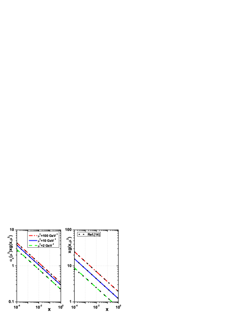
Figure 1: Left: The extracted $\alpha_{s}(\mu^{2})xg(x,\mu^{2})$ as a function of $x$ compared with the results in Ref.[14] at $\mu^{2}=2,10$ and $100~{}\mathrm{GeV}^{2}$.
Right: The extracted $xg(x,\mu^{2})$ as a function of $x$ compared with Ref.[14] at $\mu^{2}=2,10$ and $100~{}\mathrm{GeV}^{2}$.

Figure 2: Left: The extracted $\alpha_{s}(\mu^{2})xg(x,\mu^{2})$ as a function of $\mathrm{r(fm)}$ compared with the results in Ref.[14] at $x=10^{-2}..10^{-4}$.
Right: The extracted $xg(x,\mu^{2})$ as a function of $\mathrm{r(fm)}$ compared with Ref.[14] at $x=10^{-2}..10^{-4}$.

In Fig.2, we compared our results with the results in Ref.[14] for a wide range of the transverse dipole size $r$ at $x=10^{-2}..10^{-4}$. We observe that the $\alpha_{s}(\mu^{2})xg(x,\mu^{2})$ and $xg(x,\mu^{2})$ are in a very good agreement with the results in Ref.[14] in a wide range of $r$ and $x$. We see that there is a deviation between the results at large $r$ ($r>10^{-1}~{}\mathrm{fm}$) for $x=10^{-4}$. This behavior shows that saturation scale is difference on these models.
To realistically describe the structure of the proton, we must introduce a $k_{t}$ unintegrated gluon density, whose evolution at low-$x$ is governed by the BFKL equation. The object of the BFKL evolution equation at very low $x$ is the differential gluon structure function of proton

$$f(x,k_{t}^{2}) = \frac{\partial{xg(x,\mu^{2})}}{\partial{\ln}\mu^{2}}|_{\mu^{2}=k^{2}_{t}}$$ (22)

which emerges in the color dipole picture (CDP) of inclusive deep inelastic scattering (DIS). Unintegrated distributions are required to describe measurements where transverse momenta are exposed explicitly.
Using the relationship between the dipole cross-section and the unintegrated gluon distribution (i.e., Eq.(22)) it is straightforward to obtain

$$f(x,k_{t}^{2}) = \frac{3\beta_{0}\sigma_{0}}{4\pi^{2}}Q_{0}^{2}(\frac{x_{0}}{x})^{\lambda}\bigg{[}1+\frac{4{\lambda}m_{c}^{2}\ln(\frac{k_{t}^{2}}{\Lambda_{QCD}^{2}})}{k_{t}^{2}(1+\frac{4m_{c}^{2}}{k^{2}_{t}})}\bigg{]}~{}{\equiv}~{}\rho(k^{2}_{t})x^{-\lambda}.$$ (23)

The resulting UGD with the $k^{2}_{t}$-dependence and comparison with the HSS [20], IN [18] and WMR [21] models are shown in Figs. 3 and 4. In Figs.3 and 4 we plot the $k^{2}_{t}$ dependence of the UGD at $x=10^{-3}$ and $10^{-4}$, respectively.

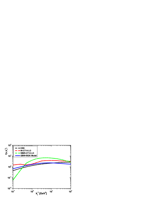
Figure 3: UGD obtained from the GBW+BGK model (solid curve) as a function of $k_{t}^{2}$ at $x=10^{-3}$, compared with the HSS [20], IN [18] and WMR [21] models.

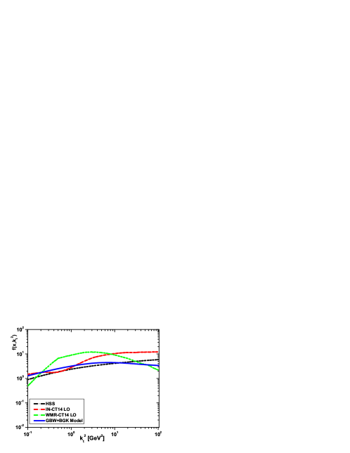
Figure 4: The same as Fig.3 for $x=10^{-4}$.

In Fig.3, the $k_{t}$ distributions of three different unintegrated gluons at $x=10^{-3}$ are shown. We observe that the GBW+BGK saturation model result, in a wide range of $k^{2}_{t}$, is comparable with the HSS and IN models. There is some suppression due to the models at large and small values of $k^{2}_{t}$. The differences are not large in a wide range of $k^{2}_{t}$ in comparison with the HSS model [20]. In Fig.4 we compared the GBW+BGK unintegrated gluons with the UGD models for $x=10^{-4}$ in a wide range of $k_{t}^{2}$. We observe that the same behavior at low values of $x$ is consistent with the UGD models in the $k_{t}$ dependence.

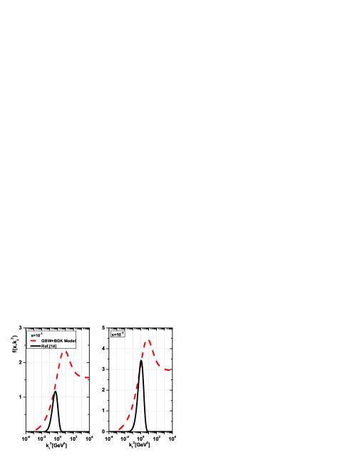
Figure 5: UGD with the GBW+BGK model as a function of $k_{t}^{2}$ compared with the results in Ref.[14] for $x=10^{-3}$ (left plot) and $x=10^{-4}$ (right plot).

In Fig.5, we compared the UGD from the GBW+BGK model with Ref.[14] in a wide range of $k_{t}^{2}$ for $x=10^{-3}$ and $10^{-4}$ respectively. We observe that $f(x,k_{t}^{2})$ in Ref.[14] is nearly symmetric. The symmetric point and the maximum of $f(x,k_{t}^{2})$ increases as $x$ decreases. We can see an enhancement then a depletion in the UGD of the GBW+BGK model with increases of $k_{t}$. The maximum of $f(x,k_{t}^{2})$ in the GBW+BGK model is larger than Ref.[14]. In the limit where $k_{t}$ approaches zero, the behavior of the UGD in the GBW+BGK and the results in Ref.[14] is similar with a different rate. In the large $k_{t}$ limit, the UGD behavior in the GBW+BGK model is almost constant (with uniform rate) where this is similar to the other UGD models (such as APIPSW [19] and IN [18] models). Indeed ,at very small $x$ ($x{\lesssim}10^{-3}$), the scaling violations in the gluon density are strong. Additionally, for large $k_{t}$, it is expected that perturbative QCD should accurately describe hard gluon radiation.

$\bullet$ Longitudinal structure function:
In the $k_{t}$-factorization, the longitudinal structure function is driven at low $x$ primarily by gluons and is related in the following form to the UGD

$$F_{L}(x,Q^{2}) = 2\frac{Q^{4}}{\pi^{2}}\sum_{f=u,d,s,c}e_{f}^{2}\int\frac{dk_{t}^{2}}{k_{t}^{4}}\int^{1}_{0}d{\beta}\int d^{2}{\mathbf{\kappa}}^{\prime}\alpha_{s}(\mu^{2})\beta^{2}(1-\beta)^{2}\frac{1}{2}\bigg{(}\frac{1}{D_{1q}}-\frac{1}{D_{1q}}\bigg{)}^{2}f(\frac{x}{z},k_{t}^{2}),$$ (24)

where $\mathbf{\kappa}^{\prime}$ is the shifted transverse momentum and the variable $\beta$ is the Sudakov parameter. They are described by the sum of the quark box (and crossed box) diagram contribution to the photon-gluon fusion [25,26] where the photon is longitudinally polarized. The variables $D_{1q}$ and $D_{2q}$ read into these parameters as reported in Ref.[26].
The on-shell limit of the $k_{t}$-factorization formula (i.e., Eq.(24)) can be described by the standard collinear factorization formula if the transverse momentum of the gluon is much smaller than the virtuality of the photon. The expression under the integral in Eq.(24) can be expanded to the first order in $k_{t}^{2}$ as

$$\bigg{(}\frac{1}{D_{1q}}-\frac{1}{D_{1q}}\bigg{)}^{2}=\frac{4\cos^{2}{\phi}\kappa^{\prime 2}k_{t}^{2}}{(\kappa^{\prime 2}+\beta(1-\beta)Q^{2}+m_{f}^{2})^{4}}.$$ (25)

Based on the strong ordering in the transverse momenta, the on-shell longitudinal structure function at the scale $\mu^{2}{\sim}Q^{2}$ is defined

$$F_{L}(x,Q^{2}) = 2\sum_{f=u,d,s,c}{e_{f}^{2}}\bigg{[}\frac{\alpha_{s}}{\pi}\int_{\overline{x}_{f}}^{1}\frac{dy}{y}(\frac{x}{y})^{2}(1-\frac{x}{y})\sqrt{1-\frac{4m_{f}^{2}x}{Q^{2}(y-x)}}yg(y,Q^{2})$$ (26)

$$-2\frac{m_{f}^{2}}{Q^{2}}\frac{\alpha_{s}}{\pi}\int_{\overline{x}_{f}}^{1}\frac{dy}{y}(\frac{x}{y})^{3}\ln\bigg{\{}\frac{1+\sqrt{1-\frac{4m_{f}^{2}x}{Q^{2}(y-x)}}}{1-\sqrt{1-\frac{4m_{f}^{2}x}{Q^{2}(y-x)}}}\bigg{\}}yg(y,Q^{2})\bigg{]}.$$

The authors in Ref.[27] presented a systematic analysis of the twist expansion in the dipole representation for the inclusive cross section based on the $k_{t}$-factorization model. the longitudinal structure function due to the leading twist-2 part in the dipole picture reads [27,28]

$$F_{L}(x,Q^{2})=\frac{1}{3\pi}\sum_{f=u,d,s,c}e_{f}^{2}\alpha_{s}xg(\xi_{L}x,Q^{2}),$$ (27)

where $\xi_{L}{\approx}2$. In order to consider the longitudinal structure function int the on-shell and the leading twist-2 models, the gluon distribution can be recovered from the GBW+BGK model (i.e., Eq.21) at the high energy limit. In Fig.6 we show our results from both models (on-shell and twist-2). We observe that both are consistent with each other. The description of data, in the region of low and moderate $Q^{2}$, is good. The $F_{L}$ structure function is plotted as a function of $x$ in bins of $Q^{2}$. Results are compared with H1 data [29,30] and the parametrization of $F_{L}(x,Q^{2})$ [31] at the LO approximation (CJ15-LO). It is seen that, for all values of the presented $Q^{2}$, the extracted longitudinal structure function with respect to the gluon distribution obtained from the GBW+BGK model, is in agreement with data. Similar investigations of the longitudinal structure function have been performed in Refs.[32-37]. In Ref.[35] an unintegrated gluon density is determined (in a similar spirit of GBW) and the longitudinal structure function is calculated and compared to data. In addition, the longitudinal structure functions in Fig.6 compared with the results $\mathrm{LLM}^{,}2023$ [35] which is determined according to the $k_{T}$-factorization and the TMD gluon densities in the proton. The LLM [35] results accompanied with the shaded bands correspond to theoretical uncertainties of the $k_{T}$-factorization connected with the choice of hard scales. The predictions are compatible with the $k_{T}$-factorization within the uncertainties.
In Fig.7, we have calculated the $Q^{2}$-dependence, at low $x$, of the longitudinal structure function at a fixed value of the invariant mass $W$, $W=230~{}\mathrm{GeV}$. Calculations have been performed from the on-shell model. Since the photon wave function depends on mass of the quarks in the $q\overline{q}$ dipole, we considered contributions to the longitudinal structure function due to the coefficients from the fixed ($n_{f}=4$) and variable $n_{f}=3+\mathrm{charm}$ active flavors. The fixed parameters in Eq.(21) are defined in the first two rows in Table 1 from Re.[15]. The extracted longitudinal structure functions are in a good agreement with the H1 data [29],in a wide range of $Q^{2}$, in both fixed parameters. We observe that the results with fixed active flavor number $n_{f}=4$ are smaller than the results with variable active flavor number $n_{f}=3+\mathrm{charm}$. However, the both results are comparable with experimental data in a wide range of $Q^{2}$.

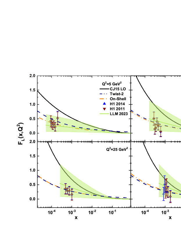
Figure 6: Longitudinal structure function extracted from the on-shell (dashed-dot curve) and twist-2 (dashed curve) models due to the gluon distribution obtained form the GBW+BGK model at fixed $Q^{2}$ as a function of $x$ variable. The results compared with the CJ15 [31] parametrization model at the LO approximation and the experimental data (up-triangle H1 2014 [29], down-triangle H1 2011 [30]) as accompanied with total errors. In addition, the results compared with the $\mathrm{LLM}^{,}2023$ [35] $k_{T}$-factorization with scale uncertainties (the green bands).

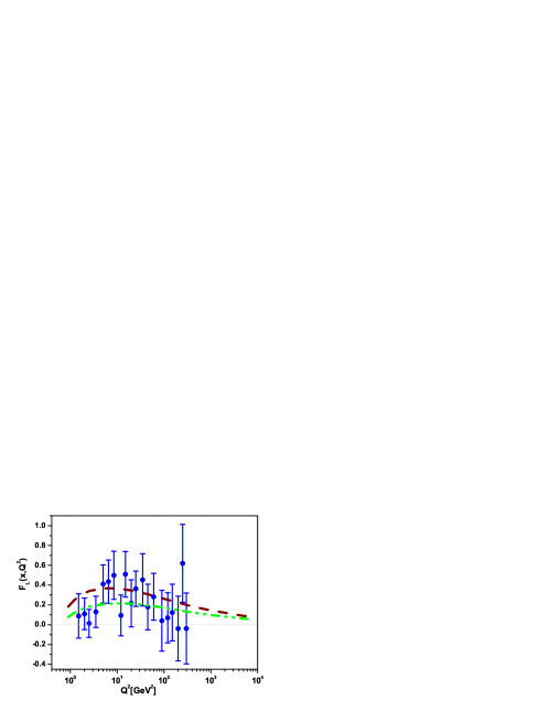
Figure 7: Longitudinal structure function extracted from the on-shell model due to the gluon distribution obtained form the GBW+BGK model as a function of variable $Q^{2}$ at fixed value of the invariant mass $\mathrm{W}=230~{}\mathrm{GeV}$. The results calculated with the fixed parameters in the dipole model [15] for $n_{f}=4$ (dashed-dot curve) and $n_{f}=3+\mathrm{charm}$ (dashed curve). Experimental data are from the H1-Collaboration [29] as accompanied with total errors.

.4 IV. Conclusion

In this paper we derive results for unintegrated color dipole gluon distribution function at small transverse momentum in the GBW+BGK model. We have shown that the $k_{t}$ factorized, evaluated within the GBW+BGK model, describes the longitudinal structure functions in the small-$x$ region, very well. In the first part of this analysis, we obtained a new description for the unintegrated gluon distribution which is close to the results in Ref.[14] for a wide range of the transverse dipole size $r$ at low $x$. We have shown, the behavior of the GBW+BGK model for the UGD is comparable with the UGD models in a wide range of $k_{t}^{2}$. In the second part of our study, we have obtained a good agreement of the proton structure function $F_{L}$, using the GBW+BGK model within the $k_{t}$-factorization framework for both on-shell and twist-2 corrections. We have analyzed the impact of the exact kinematics in the $k_{t}$-factorization scheme as they are very important for the phenomenological description of the data on $F_{L}$. In particular, it leads to larger differences in the longitudinal structure function when we consider a good fit quality with the charm and light quark contributions to the dipole coefficients. Therefore, we conclude that the GBW+BGK model provides an economical description of the data on the longitudinal structure function for fixed $W$. Explicit, analytical expressions for the integrated and unintegrated gluon distribution in the GBW+BGK model are obtained in terms of the effective parameters of the CDP and results of numerical calculations of the $F_{L}$ as well as comparisons with available experimental are presented.

.5 ACKNOWLEDGMENTS

The author is grateful to Razi University for the financial support of this project. G.R.Boroun thanks A.V. Lipatov for allowing access to data related to the longitudinal structure function with the TMD gluon density.

.6 APPENDIX

$\bullet$ $\mathbf{\mathrm{ABIPSW}~{}\mathrm{model}:}$
This is a $x$-independent model of the UGD which has been proposed by the authors in Ref.[19] as

$$f(x,k_{t}^{2})=\frac{A}{4\pi^{2}M^{2}}\Big{[}\frac{k_{t}^{2}}{M^{2}+k_{t}^{2}}\Big{]},$$ (28)

where merely coincides with the proton impact factor. Here M is a characteristic soft scale and A is the normalisation factor.

$\bullet$ $\mathbf{\mathrm{IN}~{}\mathrm{model}:}$
In the large and small $k_{t}$ regions, a UGD soft-hard model (where the soft and the hard components are defined in [18]) has been proposed by the authors in Ref. [18] as

$$f(x,k_{t}^{2})=f_{\mathrm{soft}}^{(B)}(x,k_{t}^{2})\frac{k_{s}^{2}}{k_{s}^{2}+k_{t}^{2}}+f_{\mathrm{\mathrm{hard}}}(x,k_{t}^{2})\frac{k_{t}^{2}}{k_{h}^{2}+k_{t}^{2}}.$$ (29)

$\bullet$ $\mathbf{\mathrm{HSS}~{}\mathrm{model}:}$
This model [20] is used in the study of DIS structure functions and takes the form of a convolution between the BFKL gluon Green^,s function and a leading-order (LO) proton impact factor, where has been employed in the description of single-bottom quark production at LHC and to investigate the photoproduction of $J/\Psi$ and $\Upsilon$, by the following form

$$f(x,k_{t}^{2},M_{{h}}) = \int_{-\infty}^{+\infty}\frac{d\nu}{2\pi^{2}}\mathcal{C}\frac{\Gamma(\delta-i\nu-\frac{1}{2})}{\Gamma(\delta)}(\frac{1}{x})^{\chi(\frac{1}{2}+i\nu)}(\frac{k_{t}^{2}}{Q_{0}^{2}})^{\frac{1}{2}+i\nu}\Bigg{\{}1+\frac{\overline{\alpha}_{s}^{2}\beta_{0}\chi_{0}(\frac{1}{2}+i\nu)}{8N_{c}}\log(\frac{1}{x})$$ (30)

$${\times}\Bigg{[}-\psi(\frac{1}{2}+i\nu)-\log\frac{k_{t}^{2}}{M^{2}_{{h}}}\Bigg{\}}\Bigg{]}.$$

In the above equation (i.e., Eq.(30)), $\chi_{0}(\frac{1}{2}+i\nu)$ and $\chi(\gamma)$ are respectively the LO and the next-to-leading order (NLO) eigenvalues of the BFKL kernel and $\beta_{0}=11-\frac{2}{3}n_{f}$ with $n_{f}$ the number of active quarks. Here $\overline{\alpha}_{s}=\frac{3}{\pi}\alpha_{s}(\mu^{2})$ with $\mu^{2}=Q_{0}M_{h}$ where $M_{h}$ plays the role of the hard scale which can be identified with the photon virtuality, $\sqrt{Q^{2}}$.

$\bullet$ $\mathbf{\mathrm{WMR}~{}\mathrm{model}:}$
The WMR model [21] depends on an extra-scale $\mu$, fixed at $Q$, by the following form

$$f(x,k_{t}^{2},\mu^{2}) = T_{g}(k_{t}^{2},\mu^{2})\frac{\alpha_{s}(k_{t}^{2})}{2\pi}\int_{x}^{1}dz\Bigg{[}\sum_{q}P_{gq}(z)\frac{x}{z}q(\frac{x}{z},k_{t}^{2})+P_{gg}(z)\frac{x}{z}g(\frac{x}{z},k_{t}^{2})\Theta(\frac{\mu}{\mu+k_{t}}-z)\Bigg{]},$$ (31)

where $T_{g}(k_{t}^{2},\mu^{2})$ gives the probability of evolving from the scale $k_{t}$ to the scale $\mu$ without parton emission and $P_{ij}^{,}$s are the splitting functions.

$\bullet$ $\mathbf{\mathrm{GBW}~{}\mathrm{model}:}$
This model [1] derives from the effective dipole cross section $\sigma(x,\mathbf{r})$ for the scattering of a $q\overline{q}$ pair of a nucleon by the following form

$$f(x,k_{t}^{2}) = k_{t}^{4}\sigma_{0}\frac{R_{0}^{2}(x)}{2\pi}e^{-k_{t}^{2}R_{0}^{2}(x)},$$ (32)

with $R_{0}^{2}(x)=\frac{1}{\mathrm{GeV}^{2}}(\frac{x}{x_{0}})^{\lambda}$.

I References

1. K.Golec-Biernat and M.W$\ddot{\mathrm{u}}$sthoff, Phys. Rev. D 59, 014017 (1998); K.Golec-Biernat, Acta.Phys.Polon.B 33, 2771 (2002); Acta.Phys.Polon.B 35, 3103 (2004); J.Phys.G 28, 1057 (2002).
2. J.R.Forshaw and G.Shaw, JHEP 12, 052 (2004).
3. TMD Handbook, R.Boussarie et al, arXiv [hep-ph]: 2304.03302; A.V.Lipatov, G.I.Lykasov and M.A. Malyshev, Phys.Lett.B 839, 137780 (2023).
4. Yu.L.Dokshitzer, Sov.Phys.JETP46, 641 (1977); G.Altarelli and G.Parisi, Nucl.Phys.B 126, 298 (1977); V.N.Gribov and L.N.Lipatov, Sov.J.Nucl.Phys. 15, 438 (1972).
5. V.S.Fadin, E.A.Kuraev and L.N.Lipatov, Phys.Lett.B 60, 50(1975); L.N.Lipatov, Sov.J.Nucl.Phys. 23, 338(1976); I.I.Balitsky and L.N.Lipatov, Sov.J.Nucl.Phys. 28, 822(1978).
6. R.Boussarie and Y.Mehtar-Tani, Phys.Lett.B 831, 137125 (2022).
7. E.Iancu,K.Itakura and S.Munier, Phys.Lett.B 590, 199 (2004).
8. J.Bartels, K.Golec-Biernat and H.Kowalski, Phys. Rev. D66, 014001 (2002).
9. B.Sambasivam, T.Toll and T.Ullrich, Phys.Lett.B 803, 135277 (2020).
10. J.R.Forshaw and G.Shaw, JHEP 12, 052 (2004).
11. E.Iancu, A.Leonidov and L.McLerran, Nucl.Phys.A 692, 583 (2001); Phys.Lett.B 510, 133 (2001).
12. An Assessment of U.S. Based Electron-Ion Collider Science. The National Academies Press, Washington, DC, 2018.
13. P.Agostini et al. [LHeC Collaboration and FCC-he Study Group ], J. Phys. G: Nucl. Part. Phys. 48, 110501 (2021).
14. R.S. Thorne, Phys.Rev.D71, 054024 (2005).
15. K. Golec-Biernat and S.Sapeta, JHEP 03, 102 (2018).
16. A.Luszczak and H.Kowalski, Phys.Rev.D 89, 074051 (2014).
17. A.Luszczak, M.Luszczak and W.Schafer, Phys.Lett.B 835, 137582 (2022).
18. I.P.Ivanov and N.N.Nikolaev, Phys.Rev.D 65, 054004 (2002).
19. I.V. Anikin, A. Besse, D.Yu. Ivanov, B. Pire, L. Szymanowski and S. Wallon, Phys. Rev. D 84, 054004 (2011).
20. M. Hentschinski, A. Sabio Vera and C. Salas, Phys. Rev. Lett. 110, 041601 (2013).
21. G. Watt, A.D. Martin and M.G. Ryskin, Eur. Phys. J. C 31, 73 (2003).
22. A.D.Bolognino, F.G.Celiberto, Dmitry Yu. Ivanov and A.Papa, arXiv [hep-ph]:1808.02958; arXiv [hep-ph]:1902.04520; arXiv [hep-ph]:1808.02395; F.G.Celiberto, Nuovo Cim. C 42, 220 (2019); F.G.Celiberto, D. Gordo Gomez and A.Sabio Vera, Phys.Lett.B 786, 201 (2018).
23. G.R.Boroun, Eur.Phys.J.C 83, 42 (2023); Eur.Phys.J.C 82, 740 (2022); Phys.Rev.D 108, 034025 (2023).
24. T.Goda,K.Kutak and S.Sapeta, arXiv[hep-ph]:2305.14025.
25. H. Jung, A.V.Kotikov, A.V.Lipatov and N.P.Zotov, Proc. of 15th Int. Workshop on Deep-Inelastic Scattering and Related Subjects, Munich, April 2007, arXiv[hep-ph]:0706.3793v2.
26. K.Golec-Biernat and A.M.Stasto, Phys.Rev.D 80, 014006 (2009).
27. J. Bartels, K. J. Golec-Biernat and K. Peters, Eur. Phys. J. C 17, 121 (2000).
28. N.N.Nikolaev and B.G.Zakharov, Phys.Lett.B 327, 149 (1994); Phys.Lett.B 332, 184 (1994).
29. V.Andreev, A.Baghdasaryan, S.Baghdasaryan, et al.(H1 Collab.), Eur.Phys.J.C 74, 2814 (2014).
30. F.D.Aaron, C.Alexa, V.Andreev, et al.(H1 Collab.), Eur.Phys.J.C 71, 1579 (2011).
31. A.Accardi, L.T.Brady, W.Melnitchouk, J.F.Owens and N.Sato, Phys.Rev.D 93, 114017 (2016).
32. L.P.Kaptari, A.V.Kotikov, N.Yu.Chernikova and P.Zhang, Phys.Rev.D 99, 096019 (2019).
33. S.Zarrin and S.Dadfar, Int.J.Theor.Phys. 60, 3822 (2021).
34. G.R.Boroun, Phys.Rev.D 105, 034002 (2022).
35. A.V.Lipatov, G.I.Lykasov and M.A.Malyshev, Phys.Lett.B 839, 137780 (2023).
36. R.Saikia, P.Phukan and J.K.Sarma, arXiv [hep-ph]:2304.00272.
37. Z.B.Baghsiyahi, M.Modarres and R.K.Valeshabadi, Eur.Phys.J.C 82, 392 (2022).
38. A.V.Lipatov, G.I.Lykasov, M.A.Malyshev, Phys.Rev.D 107, 014022 (2023).
39. A.V.Kotikov, A.V.Lipatov, G.Parente and N.P.Zotov, Eur.Phys.J.C 26, 51 (2002).