Asteroseismological analysis of the polluted ZZ Ceti star G 29$-$38 with TESS

Abstract

G 29$-$38 (TIC 422526868) is one of the brightest ($V=13.1$) and closest ($d=17.51$ pc) pulsating white dwarfs with a hydrogen-rich atmosphere (DAV/ZZ Ceti class). It was observed by the TESS spacecraft in sectors 42 and 56. The atmosphere of G 29$-$38 is polluted by heavy elements that are expected to sink out of visible layers on short timescales. The photometric TESS data set spans $\sim 51$ days in total, and from this, we identified 56 significant pulsation frequencies, that include rotational frequency multiplets. In addition, we identified 30 combination frequencies in each sector. The oscillation frequencies that we found are associated with $g$-mode pulsations, with periods spanning from $\sim$ 260 s to $\sim$ 1400 s. We identified rotational frequency triplets with a mean separation $\delta\nu_{\ell=1}$ of 4.67 $\mu$Hz and a quintuplet with a mean separation $\delta\nu_{\ell=2}$ of 6.67 $\mu$Hz, from which we estimated a rotation period of about $1.35\pm 0.1$ days. We determined a constant period spacing of 41.20 s for $\ell=1$ modes and 22.58 s for $\ell=2$ modes. We performed period-to-period fit analyses and found an asteroseismological model with $M_{\star}/M_{\odot}=0.632\pm 0.03$, $T_{\rm eff}=11\,635\pm 178$ K, and $\log{g}=8.048\pm 0.005$ (with a hydrogen envelope mass of $M_{\rm H}\sim 5.6\times 10^{-5}M_{\star}$), in good agreement with the values derived from spectroscopy. We obtained an asteroseismic distance of 17.54 pc, which is in excellent agreement with that provided by Gaia (17.51 pc).

1 Introduction

DAV white dwarfs (WDs), also called ZZ Ceti stars, are pulsating hydrogen (H)-rich atmosphere WDs with effective temperature in the range $10\,400{\rm K}\lesssim T_{\rm eff}\lesssim 13\,000$ K and surface gravities from $\log g\sim 7.5$ to $\sim 9$ (Winget & Kepler, 2008; Fontaine & Brassard, 2008; Althaus et al., 2010a; Córsico et al., 2019a; Saumon et al., 2022; Kilic et al., 2023). The discovery of pulsations in extremely low-mass white dwarfs extended these boundaries to cooler temperatures and lower surface gravities (Hermes et al., 2013). ZZ Ceti stars constitute the most common class of pulsating WDs, with $\sim 500$ known members to date (Bognar & Sodor, 2016; Córsico et al., 2019a; Vincent et al., 2020; Guidry et al., 2021; Romero et al., 2022). These stars are multiperiodic pulsators, showing periods in the range $100\lesssim\Pi\lesssim 1400$ s with amplitudes from 0.01 up to 0.3 magnitudes associated to spheroidal non-radial gravity ($g$) modes of low harmonic degree ($\ell=1,2$) and generally low to moderate radial order ($1\lesssim k\lesssim 15$), excited by the convective-driving mechanism (Brickhill, 1991; Goldreich & Wu, 1999). The existence of the red (cool) edge of the ZZ Ceti instability strip can be explained in terms of excited modes suffering enhanced radiative damping that exceeds convective driving, rendering them damped (Luan & Goldreich, 2018). In many cases, the ZZ Ceti pulsation spectrum exhibits rotational frequency splittings (Brickhill, 1975), which allows identifying modes and estimating the rotation period (e.g. Hermes et al., 2017).

While ground-based observations over the years have been extremely important in studying the nature of DAV stars (e.g., Landolt, 1968; Nather et al., 1990; Mukadam et al., 2004; Winget & Kepler, 2008; Fontaine & Brassard, 2008; Bradley, 2021), observations from space have revolutionized the area of ZZ Ceti pulsations (Córsico, 2020, 2022). In particular, the K2 extension (Howell et al., 2014) of the Kepler mission (Borucki et al., 2010) allowed the discovery of outbursts in ZZ Cetis close to the red edge of the instability strip (Bell et al., 2015; Luan & Goldreich, 2018), and also the discovery that incoherent pulsations (Hermes et al., 2017) can give information about the depth of the outer convection zone (Montgomery et al., 2020). In addition, the Transiting Exoplanet Survey Satellite ($TESS$; Ricker et al., 2015) has allowed the discovery of 74 new ZZ Cetis (Romero et al., 2022).

G 29$-$38, also known as ZZ Psc, WD 2326+049, EG 159, and LTT 16907, is a large-amplitude DAV star discovered to pulsate in 1974 by Shulov & Kopatskaya (1974). Its variability was confirmed a year later by McGraw & Robinson (1975), showing from the beginning of its observation a complex and extremely variable pulsational spectrum. G 29$-$38 has been the focus of numerous spectroscopic analyses. A compilation of $T_{\rm eff}$ and $\log g$ determinations can be found in Table LABEL:basic-parameters-targets, based on the Montreal White Dwarf Database (Dufour et al., 2017). It is worth noting that the latest spectroscopic determinations of $T_{\rm eff}$ and $\log g$ are more reliable given that they account for corrections based on the three-dimensional hydrodynamical atmospheric simulations by Tremblay et al. (2013). The most recent spectroscopic determination is that of McCleery et al. (2020) which gives $T_{\rm eff}=11\,296\pm 198$ K and $\log g=8.02\pm 0.03$. This effective temperature places this star near the middle of the ZZ Ceti instability strip. This star has been extensively studied for various combined properties that make it unique. G 29$-$38 was the first single WD discovered to have an infrared excess (Zuckerman & Becklin, 1987), initially interpreted as arising from a brown dwarf companion. Jura (2003) showed that infrared excess can be due to an opaque flat ring of dust within the Roche region of the WD where an asteroid could have been tidally destroyed, producing a system reminiscent of Saturn’s rings. Xu et al. (2018) showed the flux of the infrared 10 $\mu$m silicate feature increased by 10% in less than 3 years, which they interpret to be caused by an increase in the mass of dust grains in the optically thin outer layers of the disk. Cotton et al. (2020) measured the polarization of optical light from G 29$-$38 and searched for signs of stellar pulsation in the polarization data. Their data was limited and they were unable to demonstrate the impact of stellar oscillation. The importance of fingering convection due to the accretion of surrounding material by G 29$-$38 was studied by Wachlin et al. (2017). Recently, Cunningham et al. (2022) detected X rays from G 29$-$38 based on Chandra observations and derived an accretion rate higher than estimates from past studies of the photospheric abundances. Finally, Estrada-Dorado et al. (2023) revisited XMM Newton data and also found X-ray emission at the location of G 29$-$38, with spectral properties of the source similar to those detected with Chandra observations.

Beyond these very interesting features related to the environment of the star, the main characteristic of G 29$-$38 that is the focus of this paper is its pulsating nature and the possibility of probing its internal structure through asteroseismology. Bradley & Kleinman (1997) and Kleinman et al. (1998) explored the pulsation spectrum of G 29$-$38 in great detail using a time-series photometry data set spanning 10 years, deciphering for the first time the complex and ever-changing pulsational spectra of a high-amplitude DAV star. G 29$-$38 is reminiscent of cool DAVs located near the red edge of the ZZ Ceti instability strip. However, all the spectroscopic studies place the star closer to the middle of the instability strip. Kleinman et al. (1998) detected 19 independent frequencies (not counting the non-central components of the rotational multiplets) with periods spanning the interval $110-1240$ s, along with many combination frequencies. These authors plausibly suggested the harmonic degree and the radial order of 17 independent periods as being $\ell=1$ and $k=1,2,\cdots,17$, and derived a mean constant period spacing of $\Delta\Pi(\ell=1)\sim 47$ s. Further analyses of G 29$-$38 were focused on time-resolved spectrophotometry. On the one hand, van Kerkwijk et al. (2000) identified six real modes and five combination frequencies. They measured small line-of-sight velocities and detected periodic variations at the frequencies of five of the six real modes, with amplitudes of up to 5 km/s (in agreement with the expectations; Robinson et al., 1982), conceivably due to the $g$-mode pulsations. However, no velocity signals were detected at any of the combination frequencies, thus confirming for the first time that the flux variations at the combination frequencies do not reflect global pulsations, but rather are the result of non-linear processes in the outer layers of the star. On the other hand, Clemens et al. (2000) derived the harmonic degree for the six modes detected by van Kerkwijk et al. (2000), five of them (283 s, 430 s, 614 s, 653 s and 818 s) resulting from being dipole ($\ell=1$) modes, and the mode with period 776 s being a quadrupole ($\ell=2$) mode. The presence and nature of the abundant linear combinations of frequencies in the pulsation spectrum of G 29$-$38 were investigated in detail in a series of three articles by Vuille (2000a, b) and Vuille & Brassard (2000). Subsequently, Thompson et al. (2003) confirmed the measurements of the pulsation velocities detected by van Kerkwijk et al. (2000) and reaffirmed the fact that the frequency combinations and harmonics most likely result from non-linear mixing at the surface of the star and are not real modes that probe the interior, although they detected one combination mode with a significant velocity signal. Later, Thompson et al. (2008) presented optical time-series spectroscopy of G 29$-$38 taken at the Very Large Telescope (VLT). These authors estimated $\ell$ for 11 periods detected in this star, four of them being $\ell\neq 1$ modes. In particular, they derived an $\ell=3$ or $\ell=4$ value for the mode with period $\sim 353$ s.

The identification of the harmonic degree of a considerable number of modes of G 29$-$38 prompted further model grid-based asteroseismological studies based on fits to individual periods. Specifically, three independent asteroseismological analyses of G 29$-$38 were carried out. The first one was that of Castanheira & Kepler (2009), based on the mean periods of the modes from different observations from 1985 to 1993, assuming they are all $\ell=1$ modes. They found a best-fit model with $T_{\rm eff}=11\,700$ K, $M_{\star}=0.665M_{\sun}$, $M_{\rm He}=10^{-2}M_{\star}$ and $M_{\rm H}=10^{-8}M_{\star}$. The second asteroseismological analysis of this star was carried out by Romero et al. (2012), based on the same list of periods as Castanheira & Kepler (2009), but allowing $\ell$ to be 1 or 2. They found an asteroseismological model characterized by $T_{\rm eff}=11\,471$ K, $M_{\star}=0.593M_{\sun}$, $M_{\rm He}=2.39\times 10^{-2}M_{\star}$, and $M_{\rm H}=4.67\times 10^{-10}M_{\star}$. We note that, according to this asteroseismological model, 13 modes are $\ell=2$ modes and only one is an $\ell=1$ mode. The last asteroseismological analysis of this star was performed by Chen & Li (2013), who employed the 11 periods and $\ell$ identifications of Thompson et al. (2008). They found two equally valid asteroseismological models, one of them characterized by $T_{\rm eff}=11\,900$ K, $M_{\star}=0.790\,M_{\sun}$, $M_{\rm He}=10^{-2}M_{\star}$, and $M_{\rm H}=10^{-4}M_{\star}$, and the other model with $T_{\rm eff}=11\,250$ K, $M_{\star}=0.780\,M_{\sun}$, $M_{\rm He}=3.16\times 10^{-3}M_{\star}$, and $M_{\rm H}=3.16\times 10^{-6}M_{\star}$. These models are characterized by thick H envelopes, in contrast to the models of Castanheira & Kepler (2009) and Romero et al. (2012), which have H envelopes several orders of magnitude thinner.

In this work, we present new TESS observations of G 29$-$38. We also perform a detailed asteroseismological analysis of this star on the basis of the fully evolutionary models of DA WDs computed by Althaus et al. (2010b) and Renedo et al. (2010) and employed in our previous works on asteroseismology of ZZ Ceti stars (Romero et al., 2012; Romero et al., 2013; De Gerónimo et al., 2017; Romero et al., 2017; De Gerónimo et al., 2018; Romero et al., 2019, 2022). The paper is organized as follows. In Sect. 2 we describe the methods applied to obtain the pulsation periods of the target star. A brief summary of the stellar models of DA WD stars employed for the asteroseismological analysis of G 29$-$38 is provided in Sect. 3. Section 4 is devoted to the asteroseismological modeling of the target star, including the search for a possible uniform period spacing in the period spectrum, the derivation of the stellar mass using the period separation, and the implementation of a period-to-period fit with the goal of finding an asteroseismological model. Finally, in Sect. 5, we summarize our results.

Table 1: Effective temperature, surface gravity, spectral type, mass, luminosity, and cooling age measurements of G29-38 from different studies.

	$T_{\rm eff}$	$\log g$	Spectral	Mass	$\log(L_{\star}/L_{\sun})$	Cooling age	Reference
	[K]	[cgs]	type	[$M_{\odot}$]		[Gyr]
	11515$\,\pm\,$22	7.97$\,\pm\,$0.01	DA	0.59			Koester et al. (2001)
	11600	8.05	DAZ				Zuckerman et al. (2003)
	11820$\,\pm\,$175	8.15$\,\pm\,$0.05		0.70$\,\pm\,$0.03	$-2.62$	0.55	Liebert et al. (2005)
	12100	7.90	DAZ				Koester et al. (2005)
	11600	8.10	DAZ				Kilic et al. (2006)
	11485$\,\pm\,$80	8.07$\,\pm\,$0.02					Koester et al. (2009)
	12200$\,\pm\,$187	8.22$\,\pm\,$0.05	DA	0.74$\,\pm\,$0.03			Gianninas et al. (2011)
	12206$\,\pm\,$187	8.04$\,\pm\,$0.05	DAZ	0.63$\,\pm\,$0.03	$-2.50$	0.38	Giammichele et al. (2012)
	11820$\,\pm\,$100	8.4$\,\pm\,$0.1	DAZ	0.85			Xu et al. (2014)
	12020$\,\pm\,$183	8.13$\,\pm\,$0.05	DA	0.69$\,\pm\,$0.03	$-2.58$		Limoges et al. (2015)
	11956$\,\pm\,$187	8.01$\,\pm\,$0.05	DAV	0.61$\,\pm\,$0.03		0.38	Holberg et al. (2016)
	11240$\,\pm\,$360	8.00$\,\pm\,$0.03	DAZV	0.60$\,\pm\,$0.03	$-2.62$ $\,\pm\,$0.06	0.44$\,\pm\,$0.04	Subasavage et al. (2017)
	11315$\,\pm\,$180	8.02$\,\pm\,$0.06	DA	0.62$\,\pm\,$0.08			Bédard et al. (2017)
	11295.9$\,\pm\,$198	8.02$\,\pm\,$0.03	DAZ				McCleery et al. (2020)

2 Photometric observations — TESS

In this work, we investigate the pulsational properties of the well-known DAV star G 29$-$38 using the high-precision photometry of TESS (see Table LABEL:DAVlist). G 29$-$38 (TIC 422526868), $G_{\rm mag}$= 13.06) was observed by TESS in two sectors, including sector 42 (from 20 August to 16 September 2021) and sector 56 (from 01 September to 30 September 2022) in both 2 minutes and 20 seconds cadences. Using available magnitude values from the literature, we calculated the TESS magnitude of G 29$-$38 as described by Stassun et al. (2018) using the $\tt ticgen$ tool, and found $T_{\rm mag}=12.5$. The light curves were downloaded from The Mikulski Archive for Space Telescopes (MAST), which is hosted by the Space Telescope Science Institute (STScI) in FITS format. The light curves were processed by the Science Processing Operations Center (SPOC) pipeline (Jenkins et al., 2016). We downloaded the target pixel files (TPFs) of G 29$-$38 from the MAST archive with the Python package $\tt{lightkurve}$ (Lightkurve Collaboration et al., 2018). The TPFs feature an $11\times 11$ postage stamp of pixels from one of the four CCDs per camera that G 29$-$38 was located on. To ascertain the degree of crowding and any other potential bright sources close to G 29$-$38, the TPFs were analyzed. Given that the TESS pixel size is huge (21 arcsec), we checked any potential contamination through the $\tt CROWDSAP$ parameter, which provides the target flux to total flux ratio in the TESS aperture. By examining the $\tt CROWDSAP$ parameter, which is provided in Table LABEL:DAVlist, we were able to determine the level of contamination for G 29$-$38. The $\tt CROWDSAP$ value is almost 1 for both sectors, suggesting that G 29$-$38 is the source of the total flux measured by the TESS aperture. The data have previously undergone processing with the Jenkins et al. (2016) Pre-Search Data Conditioning Pipeline to eliminate common instrumental patterns. We initially extracted fluxes (“PDCSAP FLUX") and times in barycentric corrected Julian days ("BJD - 245700") from the FITS file. We then used a running 5$\sigma$ clipping mask to remove outliers. We detrended the light curves to remove any additional low-frequency systematics that may be present in the data. To do this, we applied a Savitzky–Golay filter with a three-day window length computed with the Python package $\tt lightkurve$. Finally, the fluxes were converted to fractional variations from the mean, i.e. differential intensity $\Delta I/I$, and transformed to amplitudes in parts-per-thousand (ppt). The ppt unit corresponds to the milli-modulation amplitude (mma) unit used in the past. The final light curves of G 29$-$38 from sector 42 (blue dots) and sector 56 (red dots) are shown in Fig. 1.

Table 2: List of TESS observations of G 29$-$38, including the TESS input catalog number, TESS magnitude, observed sectors, date, $\tt CROWDSAP$, and length of the runs. In addition, also listed are the temporal resolution, an average noise level of amplitude spectra, and detection threshold (which we define as the amplitude at $0.1\%$ of the FAP) which are obtained from the FT of the original and shuffled data (see text for details).

TIC	$T_{\rm mag}$	Obs.	Start Time	CROWDSAP	Length	Resolution	Average Noise	$0.1\%$ FAP
		Sector	(BJD-2 457 000)		[d]	$\mu$Hz	Level [ppt]	[ppt]
422526868	12.5	42	2447.6956	0.99	23.27	0.49	0.12	0.56
		56	2825.2625	1.00	27.88	0.42	0.11	0.51

2.1 Frequency analysis

To carry out a thorough asteroseismic study, we aim at creating a comprehensive list of each of G 29$-$38’s independent frequency and linear combination frequencies observed. In order to examine the periodicities in the data and determine the frequency of each pulsation mode, together with its amplitude and phase, Fourier transforms (FT) of the light curves were obtained. In Fig. 1, we depict the FT of sector 42 with blue lines and the FT of sector 56 with red lines.

We used our customized tool for a prewhitening procedure, which uses a nonlinear least square (NLLS) algorithm to fit each pulsation frequency in a waveform $A_{i}\sin(\omega_{i}\ t+\phi_{i})$, with $\omega_{i}=2\pi/P_{i}$, and $P_{i}$ the period. In addition, we make use of two different publicly available tools of $\tt Period04$ (Lenz & Breger, 2005) and $\tt Pyriod$ to identify the frequency of each pulsation mode. We fitted each frequency that appears above the 0.1% false alarm probability (FAP). The FAP level was calculated by reshuffling the light curves 1000 times as described in Kepler (1993). The temporal resolution of the data is about 0.49 $\mu$Hz ($1/T$, where $T$ is the data time length, which is 23.27 d) for sector 42, while the temporal resolution for sector 56 is around 0.42 $\mu$Hz as the star was observed during 27.88 d. Table LABEL:DAVlist lists all relevant information regarding the FT, including the average noise level and the $0.1\%$ FAP level of each dataset. For all the peaks that are above the accepted threshold and up to the frequency resolution of the particular dataset, we performed a non-linear least squares (NLLS) fit. This iterative process has been done starting with the highest peak until there is no peak that appears above $0.1\%$ of the FAP significance threshold. However, G 29$-$38 exhibits significant amplitude, frequency and/or phase variations over the duration of each run, resulting in an excess of power in the FT after pre-whitening. We carefully analyzed all frequencies that still had any excess power over the threshold after pre-whitening to see whether there was a close-by frequency within the frequency resolution, and only the highest amplitude frequency was fitted and pre-whitened in such cases.

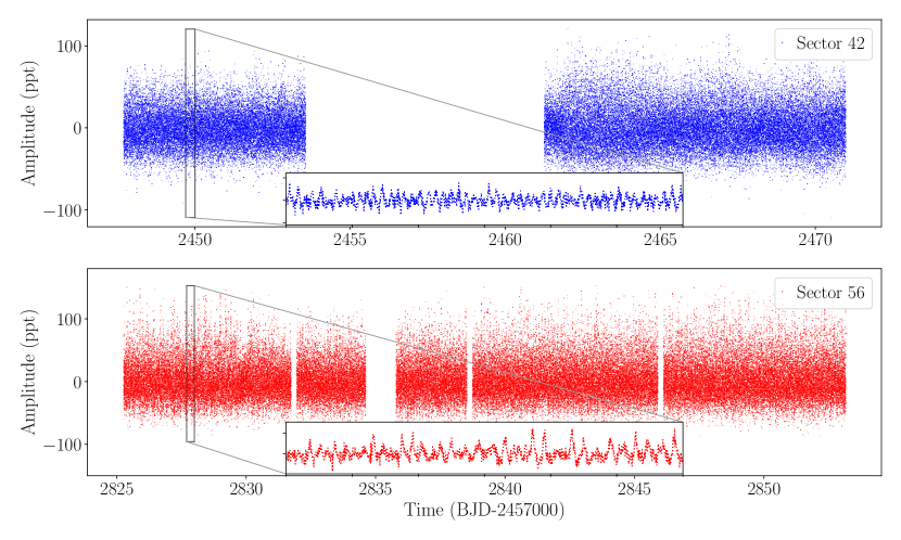
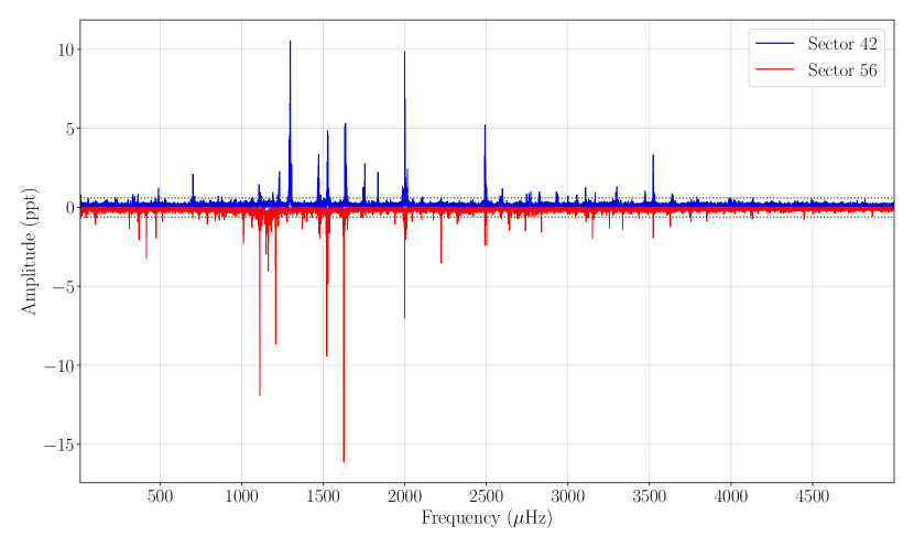
Figure 1: Top: Light curves of G 29$-$38 from sector 42 (blue dots) and sector 56 (red dots). The insets are zoom of the light curves of 0.3 days to see the rapid variability. Bottom: Fourier transforms (FTs) of G 29$-$38 computed from the sector 42 light curves (blue lines) and from the sector 56 light curves (red lines). The FT concentrates on the frequencies detected in the $g$-mode pulsation range. For the FT of sector 56, the amplitudes are inverted to improve clarity and comparison. The green dotted horizontal lines indicate the $0.1\%$ of the FAP significance threshold.

2.2 Frequency solution from sector 42

The frequency spectrum from sector 42 shows a rich content of peaks between $\sim 220$ and $4150\,\mu$Hz. We employed NLLS fits to determine the values of around 60 signals above the detection limit of 0.1% FAP = 0.56 ppt. Considering that the median noise level over the whole FT is 0.12 ppt, the observed frequencies located between 200 and $4000\,\mu$Hz have S/N between 5 and 84.

All pre-whitened frequencies for G 29$-$38 including only sector 42 are given in Table 8, showing frequencies (periods) and amplitudes with their corresponding uncertainties and the S/N ratio.

In sector 42, there is a 7.67 days gap in the light curve as can be seen in Fig. 1. We calculated the FT of each of the two halves of the light curve. The first chunk lasts for approximately 5.88 days, while the second chunk covers 9.72 days. Fig. 2 shows the FT of the first half and the second half in three panels. In the FT of the second half of the light curve, the amplitudes are inverted for clarity. The upper panel of Fig. 2 displays the short frequency region showing a notable difference in the peak located at 700 $\mu$Hz. In the second half of sector 42, the amplitude increases by a factor of two at 700 $\mu$Hz. The frequencies at 350 and 900 $\mu$Hz show both amplitude and frequency changes. The second panel of Fig. 2 displays the peaks at 1300 and 2000$\,\mu$Hz where a substantial difference was seen. Particularly, the peak at 2000 $\mu$Hz displays a triplet pattern; however, it gradually disappears at the FT of sector 42’s second half. Similarly, in the second half of sector 42, the amplitude increases by a factor of two at 1300 $\mu$Hz, and the side components of the main peak disappear. We observed significant changes in the amplitudes in the long frequency range, which is depicted in the third panel of Fig. 2, notably beyond 3250 $\mu$Hz, where all of the peaks exhibit amplitude variations.

2.3 Frequency solution from sector 56

The FT of the light curve from sector 56 reveals a plethora of peaks between 100 and 4450 $\mu$Hz. In total, 66 frequencies were detected above the detection limit of 0.1%FAP= 0.51 ppt, and were extracted from the light curve through an NLLS fit. The median noise level is 0.11 ppt and the detected frequencies have S/N values spanning from about 6 to 149. Table 9 contains all pre-whitened frequencies for G 29$-$38, including only sector 56, and provides frequencies (periods) and amplitudes with their associated uncertainties and the S/N ratio.

2.4 Combination frequencies

Combination frequencies are observed in the FTs of many $g$-mode pulsators, including low amplitude pulsating stars such as variable hot subdwarf B and WD stars, and low to large amplitude pulsators such as $\gamma$ Dor stars and slowly pulsating B stars (SPBs). Kurtz (2022) reviewed the details and feasibility of combination frequencies across the Hertzsprung-Russell Diagram of pulsating stars. Combination frequencies have been detected in several classes of pulsating WD stars, including DOVs, DBVs, and DAVs. The precise numerical correlations between combination frequencies and their parent frequencies are used to identify them. The frequency combination peaks are not self-excited, but rather result from nonlinear processes linked with the surface convection zone and can be used to infer the latter’s thermal response timescale (Montgomery, 2005).

Both sectors have numerous combination frequencies. TESS observations resolve around 30 combination frequencies per sector. A complete list of combination frequencies is provided in Tables 8 and 9, for sectors 42 and 56, respectively. In order to count as a combination frequency, we made two assumptions. First, we assumed that linear combinations have lower amplitudes than their parent frequencies. Second, we designated a combination frequency if the difference between the parent and combination frequency was within the frequency resolution of $\sim$ 0.5 $\mu$Hz.

In the case of sector 42, we detected 30 combination frequencies, and $\sim$93% of which were located either in the short- ($\leq$ 800 $\mu$Hz) or long-frequency ($\geq$ 2750 $\mu$Hz) regions, as illustrated with grey shaded regions in Fig. 3. In this plot, the location of each combination frequency is shown with a vertical dashed green line. We detected only two combination frequencies out of these regions, at 1193 and 2223 $\mu$Hz. While the mean S/N of the parent peaks corresponds to 24, the mean of S/N of the combination frequencies corresponds to 7.

As seen in the grey shaded regions of Fig. 4, we identified 29 combination frequencies for sector 56, and around 90 percent of them were found in the short- ($\leq$ 900 $\mu$Hz) and long-frequency ($\geq$ 2610 $\mu$Hz) regions. Out of these two areas, only three frequencies at 1733, 2176, and 2322 $\mu$Hz were detected. The precise location of each combination frequency is presented in Fig. 4 with the vertical dashed green line. The mean S/N of combination frequencies in this case, however, equates to 11, whereas the mean S/N of parent peaks corresponds to 27.

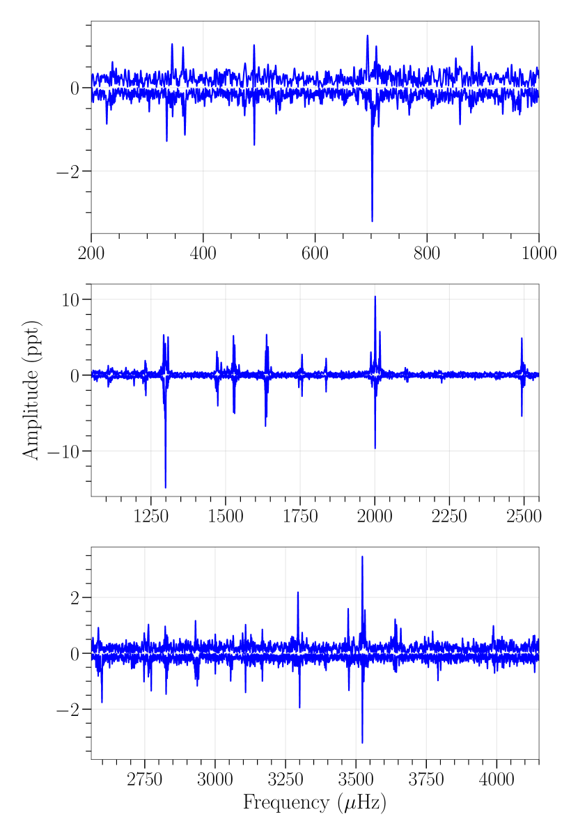
Figure 2: FT of the first and second half of sector 42, displaying amplitude changes during the 23 d observation. The amplitudes of the second half are inverted for improved clarity and comparison.

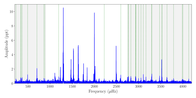
Figure 3: FT of sector 42, showing the location of combination frequencies (vertical dotted green lines). The low ($\leq$ 900 $\mu$Hz) and high ($\geq$ 2750 $\mu$Hz) frequency regions, which are depicted as grey-shaded areas, are where the majority of the combination peaks are found.

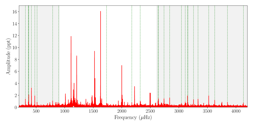
Figure 4: FT of sector 56, showing the location of combination frequencies (vertical dotted green lines). The low ($\leq$ 900 $\mu$Hz) and high ($\geq$ 2610 $\mu$Hz) frequency regions, which are depicted as grey-shaded areas, are where the majority of the combination peaks are found.

2.5 Mode identification

To constrain the internal structure of G 29$-$38 with asteroseismology, our primary goal is to identify the modes of the observed pulsations. The nonradial pulsation modes are characterized by three quantized numbers, $k,\ell$, and $m$, where $k$ represents the number of radial nodes between the center and the surface, $\ell$ the number of nodal lines on the surface, and $m$ the azimuthal order, which denotes the number of nodal great circles connecting the star’s pulsation poles. To identify the pulsational modes of G 29$-$38, we applied two methods, namely rotational multiplets, and asymptotic period spacing, as discussed in the following sections.

2.6 Rotational multiplets

Rotational multiplets can be used to ascertain the rotation period and pinpoint the pulsation modes in rotating stars when nonradial oscillations are present (Cox, 1980; Unno et al., 1989; Aerts et al., 2010; Catelan & Smith, 2015, and references therein).

The eigenfrequencies of harmonic degree $\ell$ break into $2{\ell}+1$ components that differ in azimuthal ($m$) number owing to slow stellar rotation, which is a well-known feature of nonradial stellar pulsations. When the rotation is slow and rigid, the frequency splitting is $\delta\nu_{\ell,k,m}=m\ (1-C_{\ell,k})\ \Omega_{\rm R}$, $\Omega_{\rm R}$ being the rotational angular frequency of the pulsating star and $m=0,\pm 1,\pm 2,\cdots,\pm\ell$ (e.g. Unno et al., 1989). The slow rotation requirement means that $\Omega_{\rm R}\ll\nu_{\ell,k}$. The $C_{\ell,k}$ constants are the Ledoux coefficients (Ledoux & Walraven, 1958), which may be calculated as $C_{\ell,k}\sim[\ell(\ell+1)]^{-1}$ in the asymptotic limit of high-order $g$ modes ($k\gg\ell$). In the asymptotic limit, $C_{1,k}\sim 0.5$ and $C_{2,k}\sim 0.17$ in the case of $\ell=1$ and $\ell=2$ modes, respectively. Multiplets in the frequency spectrum of a pulsating WD are highly valuable for identifying the harmonic degree of the pulsation modes, in addition to enabling an estimate of the rotation period of nonradial pulsating stars. Rotational multiplets have been found in all classes of pulsating WDs, including GW Vir, DBV, and DAV stars, with calculated rotation periods ranging from an hour to a few days. The method’s application and recent examples can be found in Hermes et al. (2017); Córsico et al. (2022b); Uzundag et al. (2022); Oliveira da Rosa et al. (2022) and Romero et al. (2023).

Since the FTs from both sectors show different structures, we interpreted each FT separately to search for rotational triplets and quintuplets. In the FT of sector 42, we found three distinct triplets, whose central components ($m\,=\,0$) are located at 1637.552, 1750.641, and 2497.176 $\mu$Hz, with an average splitting of $\delta\nu=4.83\,\mu$Hz. We depict these three triplets in the third to fifth panel of Fig. 5, along with the window function (sixth panel) and a doublet at 1526.59 and 1530.251 $\mu$Hz (second panel). Among these three multiplets, the only triplet that is found in the FT of sector 56, is located at 2497.176 $\mu$Hz. This triplet was also detected by Kleinman et al. (1998). The other ones are either completely absent or incomplete, showing two components in the FT of sector 56. For instance, the triplet with central components at 1637.552 and 1750.641 $\mu$Hz is absent. However, two additional peaks appear at 1628.166 and 1649.424 $\mu$Hz, making the interpretation difficult. These two peaks might be independent of the triplet that is resolved in the FT of sector 42, or they could be interpreted as rotational quintuplets. However, in that case, the splittings are inconsistently spanning from 3.76 $\mu$Hz to 7.04 $\mu$Hz. Thus, based on the FT from sector 42, we assessed 1633.792, 1637.552, and 1642.383 $\mu$Hz as rotational triplets. The doublet detected at 1526.59 and 1530.251 $\mu$Hz becomes complete when the FT from sector 56 is included. This region was also resolved in the dataset provided by Kleinman et al. (1998), indicating that rotational multiples may exist, although their data were equally inconclusive. Lastly, in the first panel of Fig. 5, we showed another candidate at 1106.833, 1111.944, and 1115.196 $\mu$Hz, with a splitting of 5.11 and 3.25 $\mu$Hz, respectively. All these candidates are listed in Table 3 with their rotational splittings ($\delta\nu$). Overall, the splitting for $\ell=1$ modes from 3.73 $\mu$Hz to 5.43 $\mu$Hz provides a mean rotation period range between 1.07 and 1.55 days. If we include all these five candidates as potential rotational multiples, then the average splitting is $\delta\nu=4.57\,\mu$Hz. This provides a rotation period for G 29$-$38 of $\sim$1.24 days, which aligns with what was reported by Kleinman et al. (1998).

Once we determine the $\ell=1$ triplets, we may look for modes with higher modal degrees. According to the previously mentioned Ledoux formula, the splitting in $\ell=2$ quintuplets is $\sim 1.67$ times larger than in $\ell=1$ triplets, which range from 3.73 to 5.43 $\mu$Hz. In the case of $\ell=2$ quintuplets, higher modal degree modes will have even larger splittings, ranging from 6.23 to 9.07 $\mu$Hz. The structure of the candidates of rotational quintuplets is complex, as shown in Fig. 6, probably due to the detected amplitude modulation. We found only one candidate with a complete structure showing 5 azimuthal orders from 1986.868 ($m=-2$) to 2016.62 $\mu$Hz ($m=+2$) and average splitting of $\delta\nu=6.77\,\mu$Hz, which is shown in the sixth panel in Fig. 6. None of the remaining candidates show the complete structure, and the components vary sector by sector as in the case of dipole multiplets. The splittings for $\ell=2$ modes (except for a quintuplet at 1999.742  $\mu$Hz) span from 6.17 to 8.42 $\mu$Hz with an average splitting of $\delta\nu=6.81\,\mu$Hz. Taking into account all these six candidates as quintuplets, the average splitting is $\delta\nu=6.66\,\mu$Hz. This provides a mean rotation period for G  29$-$38 of $\sim$1.45 days.

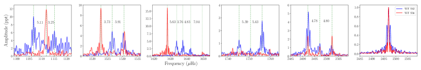
Figure 5: The amplitude spectra of G 29$-$38 that is calculated based on sector 42 (blue lines) and sector 56 (red lines) showing rotational triplets. The first sub-figure presents the window function of G 29$-$38 with the same color code centered at 1526.59 $\mu$Hz for comparison. The remaining sub-plots display rotational splittings in four different regions in the amplitude spectra, with an average splitting of $\delta\nu=4.57\,\mu$Hz.

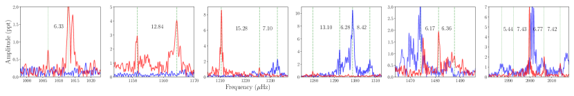
Figure 6: Same as in Fig. 5 to display rotational quintuplets. The sub-plots present rotational splittings in three different regions in the amplitude spectrum, with an average splitting of $\delta\nu=6.66\,\mu$Hz for $\ell=2$ modes. See text for more details.

2.7 Asymptotic period spacing

The periods of $g$-modes with consecutive radial order are roughly evenly separated (e.g. Tassoul et al., 1990) in the asymptotic limit of high radial orders ($k\gg\ell$), being the constant period spacing dependent on the harmonic degree:

$$\Delta\Pi_{\ell}^{\rm a}=\frac{{\Pi}_{0}}{\sqrt{\ell(\ell+1)}},$$ (1)

$\Pi_{0}$ being a constant value defined as

$$\Pi_{0}=\frac{2\pi^{2}}{\left[\int_{r_{1}}^{r_{2}}\frac{N}{r}dr\right]},$$ (2)

where $N$ is the Brunt-Väisälä frequency. The asymptotic period spacing given by Eq.(̃1) is very close to the computed period spacing of $g$-modes in chemically homogeneous stellar models without convective regions (Tassoul, 1980). In the case of DAVs, the asymptotic period spacing (and of course, also the average of the computed period spacings) is a function of the stellar mass, the effective temperature, and the thickness of the H envelope, with similar degrees of sensitivity to each parameter (Tassoul et al., 1990). This implies that measuring a period spacing in G 29$-$38 can be useful for identifying the harmonic degree of the observed frequencies, but caution should be exercised in using it to derive an estimate of stellar mass, due to the simultaneous dependence of the period spacing on $M_{\star}$, $T_{\rm eff}$, and $\log(M_{\rm H}/M_{\star})$. The latter does not happen in the case of DBVs and GW Vir stars, since for them, the period spacing is basically dependent only on $T_{\rm eff}$ and $M_{\star}$ (Córsico et al., 2021, 2022a, 2022b). That said, however, in Sect. 4.1 we will show that it is still feasible to derive a range of stellar mass values for G 29$-$38 on the basis of the observed period spacing, disregarding the exact value of $T_{\rm eff}$ and $M_{\rm H}$.

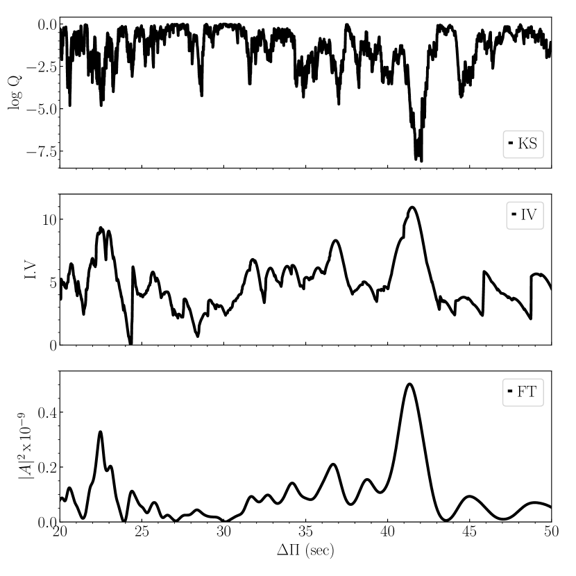
Figure 8: K-S (upper panel), I-V (middle panel), and F-T (bottom panel) significance tests to search for a constant period spacing in the case of G 29$-$38. The tests are applied to the pulsation periods in Table 3. A period spacing of $\sim 41$ s is evident.

In Fig. 7, we show the pulsation spectrum of G 29$-$38 in terms of the periods. The vertical red lines (blue lines) indicate the location of $\ell=1$ ($\ell=2$) periods that produce the patterns of constant dipole and quadrupole period spacings. We searched for a constant period spacing in the data of G 29$-$38 using the Kolmogorov-Smirnov (K-S; Kawaler, 1988), the inverse variance (I-V; O’Donoghue, 1994), and the Fourier Transform (F-T; Handler et al., 1997) significance tests. In the K-S test, the quantity $Q$ is defined as the probability that the observed periods are randomly distributed. Thus, any uniform or at least systematically non-random period spacing in the period spectrum of the star will appear as a minimum in $Q$. In the I-V test, a maximum of the inverse variance will indicate a constant period spacing. Finally, in the F-T test, we calculate the FT of a Dirac comb function (created from a set of observed periods), and then we plot the square of the amplitude of the resulting function in terms of the inverse of the frequency. A maximum in the square of the amplitude will indicate a constant period spacing. Fig. 8 displays the results of applying the three significance tests to the period spectrum of G 29$-$38. We adopted the full set of 57 periods of Table 3. The three tests point to the existence of a clear pattern of $\ell=1$ constant period spacing of $\Delta\Pi\sim 41$ s.

To derive a refined value of the period spacing, the identified 12 $\ell=1$ and 15 $\ell=2$ modes were used to obtain the mean period spacing through an LLS fit. We note that the uncertainties associated with the measurements might be underestimated because some of the pulsational modes are members of incomplete rotational triplets or quintuplets in which we cannot assess the central component ($m=0$) of the modes. Therefore, to accurately assess the actual uncertainty, we performed fits on 1000 permutations of the periods as described in Bell et al. (2019) and Uzundag et al. (2021). In each fit, we randomly assigned a value of $m\in\{-1,0,1\}$ for triplets and $m\in\{-2,-1,0,1,2\}$ for quintuplets to every observed mode and then adjusted to the intrinsic value of $m=0$ using an assumed rotational splitting. The distribution of each fit is shown in the fourth panel of Fig. 9. By calculating the standard deviation of the best-fit slopes, which amounts to 0.96 s for dipole modes and 1.02 s for quadrupole modes, we accounted for additional uncertainty. We obtain a period spacing of $\Delta\Pi_{\ell=1}=41.20^{+1.98}_{-1.92}$ s and $\Delta\Pi_{\ell=2}=22.58^{+2.00}_{-2.05}$ s. Our findings align with the value derived from the three significance tests conducted directly on the list of periods. In the second and third panels of Fig. 9 we show the residuals ($\delta\Pi$) between the observed dipole periods ($\Pi_{i}^{\rm O}$) and the periods derived from the mean period spacing ($\Pi_{\rm fit}$). The presence of two minima between $k=20$ and 25 for $\ell=1$, and $k=25$ and 35 for $\ell=2$ in the distribution of residuals suggests the occurrence of mode-trapping effects inflicted by the presence of internal chemical transition regions.

Table 3: Detected frequencies, periods, and amplitudes (and their uncertainties) and the signal-to-noise ratio with identified pulsational modes along with rotational splittings.

$\nu$	$\Pi$	$A$	S/N	$k$	$\ell$	$m$	$\delta\nu$
($\mu$Hz)	(s)	(ppt)					$\mu$Hz
740.059* (21)	1351.244 (13)	0.742 (69)	6.9
838.89* (18)	1192.051 (12)	0.857 (69)	7.9	32	1
864.037* (19)	1157.358 (12)	0.801 (69)	7.4	31	1
1006.627* (19)	993.417 (11)	0.834 (69)	7.7	47	2	+1	6.33
1012.964* (07)	987.202 (10)	2.268 (69)	21.0	47	2	0
1064.336* (13)	939.553 (11)	1.216 (69)	11.3	26	1
1106.833 (17)	903.478 (14)	1.458 (10)	11.7	25	1	+1	5.11
1111.944* (05)	899.326 (10)	11.84 (47)	109.8	25	1	0
1115.196 (33)	896.712(27)	0.900 (13)	7.5	25	1	$-1$	3.25
1151.511* (06)	868.424 (10)	2.801 (69)	25.9	41	2	$-2$	12.84
1164.353* (04)	858.846 (10)	4.056 (69)	37.6	41	2	0
1181.656* (10)	846.270 (10)	1.49 (69)	13.8	24	1
1210.47* (02)	826.125 (10)	8.668 (69)	80.4	39	2	+2	15.28
1225.755* (30)	815.824 (12)	1.085 (10)	10.1	39	2	0
1232.854 (11)	811.125 (77)	2.197 (10)	17.6	39	2	$-1$	7.10
1279.511* (17)	781.549 (11)	0.914 (69)	8.5	37	2	+2	13.10
1292.603 (41)	773.646 (79)	4.240 (13)	35.3	37	2	0
1298.883 (02)	769.892 (14)	10.544 (10)	84.4	37	2	$-1$	6.28
1307.303 (15)	764.942 (66)	2.627 (13)	21.9	37	2	$-2$	8.42
1371.426* (12)	729.168 (10)	1.315 (69)	12.2	35	2
1401.587* (18)	713.477 (10)	0.85 (69)	7.9	21	1
1431.995* (25)	698.327 (11)	0.612 (69)	5.7	34	2
1475.167* (10)	677.889 (10)	1.627 (69)	15.1	33	2	+1	6.17
1481.34* (08)	675.065 (10)	1.906 (69)	17.7	33	2	0
1487.704* (14)	672.177 (10)	1.074 (69)	9.9	33	2	$-1$	6.36
1522.859* (02)	656.660 (10)	9.462 (69)	87.7	19	1	+1	3.73
1526.590 (05)	655.054 (22)	4.983 (10)	39.9	19	1	0
1530.651* (03)	653.317 (10)	4.959 (69)	45.9	19	1	$-1$	3.91
1539.918* (11)	649.385 (10)	1.467 (69)	13.6	32	2
1628.166* (01)	614.188 (10)	16.122 (69)	149.4	30	2
1633.792 (05)	612.073 (19)	5.018 (10)	40.2	18	1	+1	3.76
1637.552 (05)	610.667 (19)	5.035 (10)	40.3	18	1	0
1642.383 (09)	608.871 (36)	2.640 (10)	21.1	18	1	$-1$	4.83
1649.424* (11)	606.272 (10)	1.346 (69)	12.5
1745.251 (18)	572.983 (62)	1.339 (10)	10.7	17	1	+1	5.39
1750.641 (36)	571.219 (11)	0.696 (10)	5.6	17	1	0
1756.076 (09)	569.451 (29)	2.796 (10)	22.4	17	1	$-1$	5.43
1836.735 (11)	544.444 (34)	2.186 (10)	17.5	27	2
1940.523* (15)	515.325 (10)	1.064 (69)	9.9	26	2
1986.868 (11)	503.304 (26)	1.261 (13)	10.5	25	2	+2	5.44
1992.310 (48)	501.930 (12)	0.687 (69)	6.3	25	2	+1	7.43
1999.742* (02)	500.065 (10)	6.948 (69)	64.4	25	2	0
2006.51* (09)	498.378 (10)	1.811 (69)	16.8	25	2	$-1$	6.77
2013.93* (12)	496.542 (10)	1.274 (69)	11.8	25	2	$-2$	7.42
2016.620 (26)	495.879 (63)	2.476 (11)	23.1			-
2045.91* (18)	488.780 (10)	0.853 (69)	7.9	15	1
2104.979* (27)	475.064 (62)	0.809 (99)	7.5	24	2
2223.76* (04)	449.689 (10)	3.499 (69)	32.4	14	1
2327.068* (18)	429.725 (10)	0.881 (69)	8.2	22	2
2492.399 (04)	401.219 (08)	5.216 (10)	41.7	13	1	+1	4.78
2497.176* (17)	400.452 (28)	1.455 (10)	11.7	13	1	0
2502.278* (07)	399.636 (10)	2.345 (69)	21.7	13	1	$-1$	4.80
2594.995* (21)	385.357 (10)	0.741 (69)	6.9	20	2
3754.433* (17)	266.352 (10)	0.893 (69)	8.3
The frequencies that are detected in sector 42 are unmarked.
The frequencies that are detected in sector 56 are marked with an asterisk.

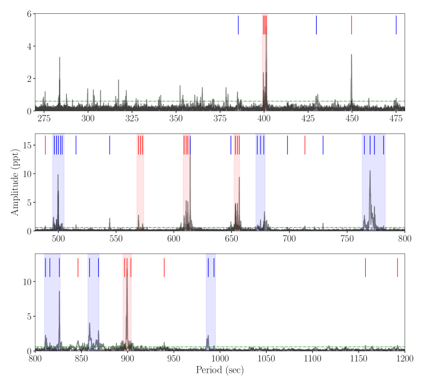
Figure 7: Pulsation spectrum of G 29$-$38 in terms of the periods based on combined sectors 42 and 56. The vertical red lines (blue lines) indicate the location of $\ell=1$ ($\ell=2$) periods that make up the patterns of constant dipole and quadrupole period spacings. The vertical red (blue) shaded regions correspond to the potential rotational multiples (quintuplets) that are zoomed in Figs. 5 and 6 in the frequency domain. The horizontal blue lines show the confidence level of 0.1% FAP which is calculated based on sector 42. Detected modes are labeled in Table 3.

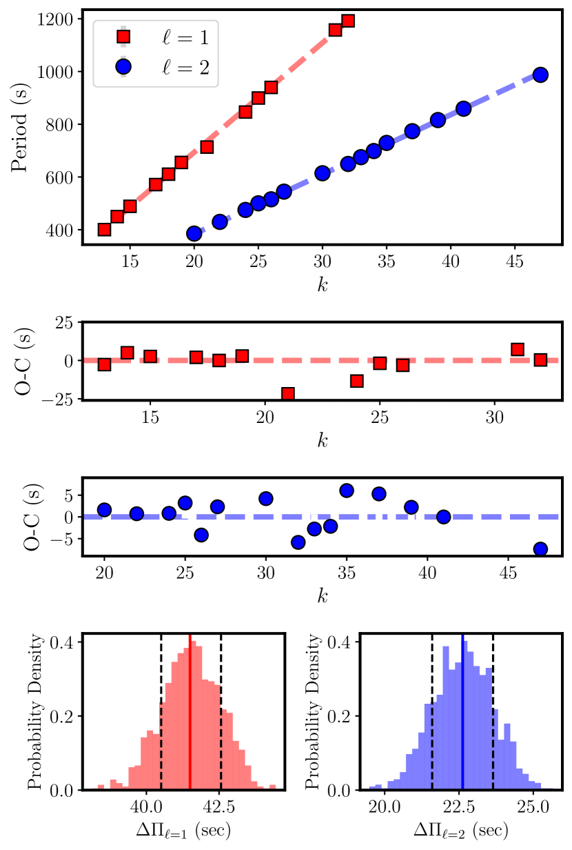
Figure 9: Linear least-squares fit the periods of G 29$-$38 marked with filled red squares ($\ell=1$) and blue dots ($\ell=2$). The derived period spacing from this fit is $\Delta\Pi_{\ell=1}=41.20$ s and $\Delta\Pi_{\ell=2}=22.58$ s. The residuals for $\ell=1$ modes (second panel) and $\ell=2$ modes (third panel) of the period distribution relative to the mean period spacing. The fourth panel shows the distribution of the resulting fits for $\ell=1$ modes (left panel) and $\ell=2$ modes (right panel). The lower and upper bounds, which are shown with vertical dashed black lines are calculated by determining the 16th and 84th percentiles of each distribution. The derived mean period spacing corresponds to the 50th percentiles, which are shown with a vertical red line for $\ell=1$ modes and a vertical blue line for $\ell=2$ modes. Note that the radial order $(k)$ assignation has been done arbitrarily, see Sect. 2.7 for more details on mode identification and the mean period spacing computations.

3 Evolutionary models

The asteroseismological analysis presented in this work is based on full DA WD evolutionary models that consider the complete evolution of the progenitor stars. Specifically, the models adopted here are taken from Althaus et al. (2010b) generated with the LPCODE evolutionary code. LPCODE computes the complete evolution of the WD progenitor from the main sequence, through the hydrogen and helium burning stages, the thermally pulsing and mass-loss stages on the AGB, and the WD cooling phase. Thus, these models are characterized by consistent chemical profiles for both the core and envelope. The models adopt the convection scheme ML2 with the mixing length parameter $\alpha=1$ (Bohm & Cassinelli, 1971; Tassoul et al., 1990). For details regarding the input physics and the evolutionary code, we refer the reader to the works of Althaus et al. (2010b) and Renedo et al. (2010). These evolutionary tracks and models have been successfully employed in previous studies of hydrogen-rich pulsating WDs (see. e.g., Althaus et al., 2010b; De Gerónimo et al., 2017, 2018; Romero et al., 2012; Romero et al., 2013; Romero et al., 2017, 2019, 2022). In this work, we consider a model grid of carbon-oxygen core WDs with stellar masses varying from 0.525 to 0.877$M_{\odot}$ with total helium content of $M_{\rm He}\sim 10^{-2}M_{\star}$ and hydrogen content ($M_{\rm H}$) varying from $10^{-4}$ to $10^{-9}M_{\star}$ (see Table 4). Once the models reach the ZZ Ceti instability strip, non-radial $\ell=1,2$ $g$-mode periods are computed for each model. This is done employing the adiabatic version of the LP-PUL pulsation code (Córsico & Althaus, 2006).

From the previous spectroscopic determinations of $\log g$ and $T_{\rm eff}$, shown in Table LABEL:basic-parameters-targets, we derived an average effective temperature and $\log g$ of $11\,738\pm 162$ K and $8.08\pm 0.04$, respectively. In Fig. 10 we show the spectroscopic measurements in the $T_{\rm eff}-\log g$ plane as well their average and previous asteroseismic determinations. Superimposed on these, we also show our canonical evolutionary sequences and our best-fit model (see next section). By interpolating on our grid of evolutionary tracks, we found that the average values of $T_{\rm eff}$ and $\log g$ of G 29$-$38 are compatible with a WD model with $M_{\star}=0.651\,M_{\odot}$ if the canonical H envelopes are assumed. The total H content of our DA WD models is treated as a free parameter.

4 Asteroseismic analysis

Our asteroseismological analysis consists in searching for the model that best matches the pulsation periods of our target star, G 29$-$38. To this end, we seek the theoretical model whose period spectrum minimizes a quality function defined as the average of the absolute differences between theoretical and observed periods. This method has been successfully applied in previous works of the La Plata Stellar Evolution and Pulsation Research Group for a wide variety of classes of pulsators (Romero et al., 2012; Romero et al., 2013; Romero et al., 2017; Córsico et al., 2019b; Córsico et al., 2022b, a, and references therein).

Before describing the seismological analysis, we extract information on the stellar mass range of G 29$-$38 using the observed period spacing below.

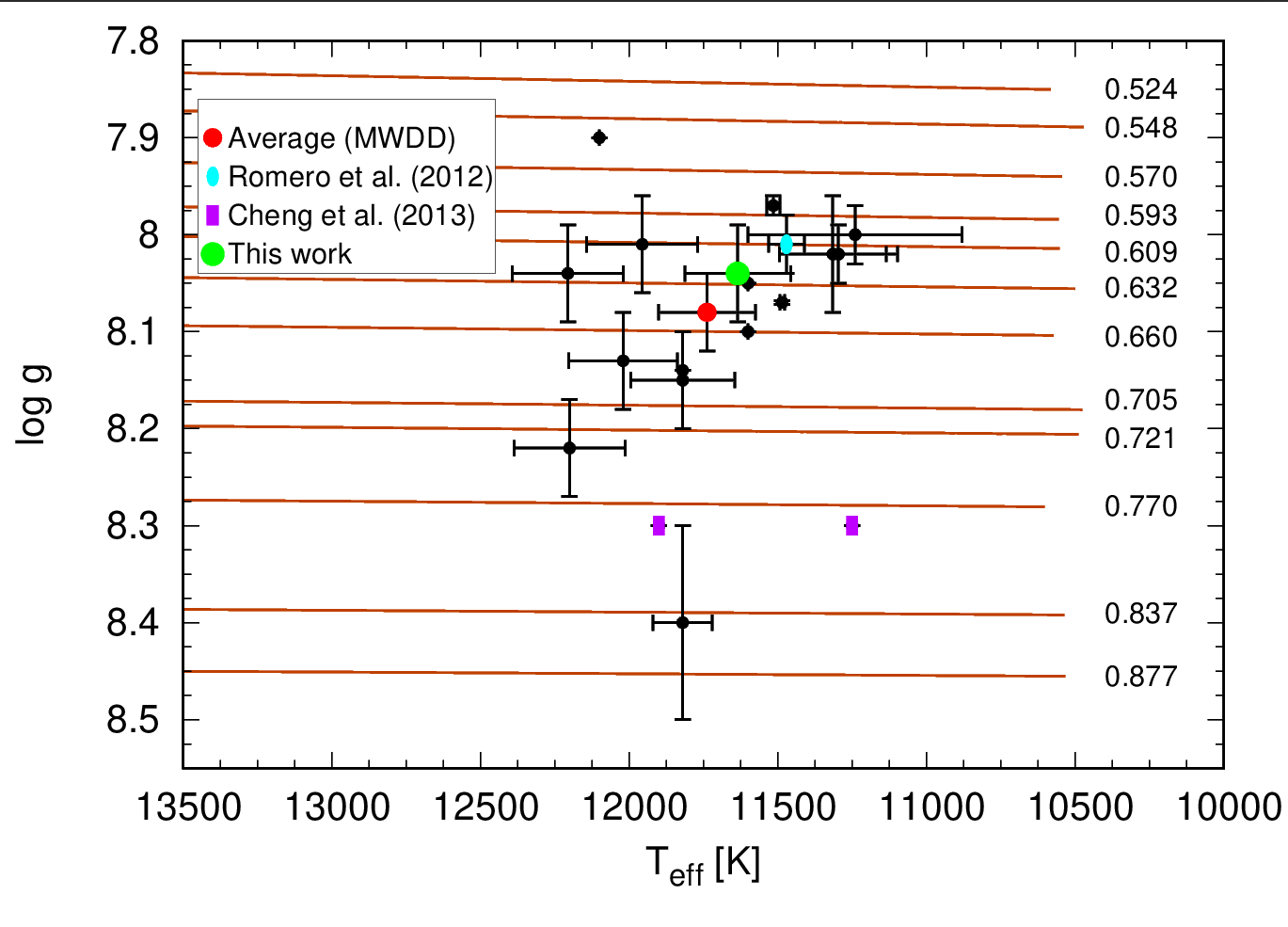
Figure 10: Determinations of $\log g$ and $T_{\rm eff}$ (black dots) for G 29$-$38 from the Montreal White Dwarf Database (see the compilation in Table LABEL:basic-parameters-targets) together with their average (red circle), our asteroseismic solution (green circle), and asteroseismic solutions from previous works (cyan ellipse and magenta rectangles). Superimposed on these, we plot each of our canonical evolutionary sequences and their corresponding value of stellar mass in solar units (red lines)

4.1 The stellar mass of G 29$-$38 compatible with the observed period spacing

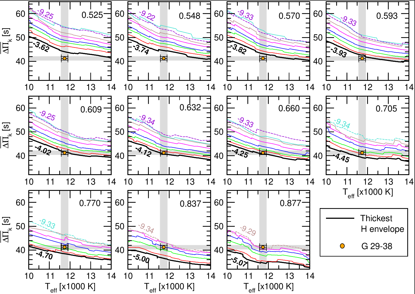
Figure 11: Average of the computed dipole ($\ell=1$) period spacings, $\overline{\Delta\Pi_{k}}$, in terms of the effective temperature, for different stellar masses in solar units (numbers at the top right corner of each panel) and thicknesses of the H envelope (see Table 4 for the specific values of $\log(M_{\rm H}/M_{\star})$) drawn with different colors. In each panel, we include numbers along two curves, which correspond to the value of $\log(M_{\rm H}/M_{\star})$ for the thickest (black thick curves) and the thinnest (violet, turquoise, and brown thin dashed curves, depending on $M_{\star}$) H envelopes for each stellar mass value. The location of G 29$-$38 is emphasized with an orange circle with error bars ($T_{\rm eff}=11\,738\pm 162$ K and $\Delta\Pi=41.20^{+1.98}_{-1.92}$ s). The gray bands correspond to the uncertainties in $T_{\rm eff}$ and $\Delta\Pi$ of G 29$-$38.

Table 4: The values of the stellar mass of our set of DA WD models (upper row) and the mass of H corresponding to the different envelope thicknesses considered for each stellar mass. The second row shows the maximum value of the thickness of the H envelope for each stellar mass (the “canonical” envelope thickness) according to our evolutionary computations.

$M_{\star}/M_{\sun}$	0.525	0.548	0.570	0.593	0.609	0.632	0.660	0.705	0.721	0.770	0.837	0.877
$\log(M_{\rm H}/M_{\star})$	$-3.62$	$-3.74$	$-3.82$	$-3.93$	$-4.02$	$-4.12$	$-4.25$	$-4.45$	$-4.50$	$-4.70$	$-5.00$	$-5.07$
	$-4.27$	$-4.27$	$-4.28$	$-4.28$	$-4.45$	$-4.46$	$-4.59$	$-4.88$	$\cdots$	$-4.91$	$-5.41$	$-5.40$
	$-4.85$	$-4.85$	$-4.84$	$-4.85$	$-4.85$	$-4.86$	$-4.87$	$-5.36$	$-5.36$	$-5.37$	$-6.36$	$-6.39$
	$-5.35$	$-5.35$	$-5.34$	$-5.34$	$-5.35$	$-5.35$	$-5.35$	$-6.35$	$-6.43$	$-6.35$	$-7.36$	$-7.38$
	$-6.33$	$-6.35$	$-6.33$	$-6.33$	$-6.34$	$-6.34$	$-6.35$	$-7.35$	$-7.34$	$-7.34$	$-8.34$	$-8.37$
	$-7.34$	$-7.33$	$-7.34$	$-7.34$	$-7.33$	$-7.35$	$-7.33$	$-8.34$	$-8.33$	$-8.33$	$-9.34$	$-9.29$
	$-8.33$	$-8.33$	$-8.31$	$-8.33$	$-8.33$	$-8.33$	$-8.33$	$-9.34$	$-9.24$	$-9.33$	$\cdots$	$\cdots$
	$-9.25$	$-9.22$	$-9.33$	$-9.33$	$-9.25$	$-9.34$	$-9.33$	$\cdots$	$\cdots$	$\cdots$	$\cdots$	$\cdots$

A useful method to infer the stellar mass of pulsating WD stars is to compare the measured period spacing ($\Delta\Pi$) with the average of the computed period spacings ($\overline{\Delta\Pi_{k}}$). This last quantity is calculated as $\overline{\Delta\Pi_{k}}=(n-1)^{-1}\sum_{k}\Delta\Pi_{k}$, where the “forward” period spacing ($\Delta\Pi_{k}$) is defined as $\Delta\Pi_{k}=\Pi_{k+1}-\Pi_{k}$ ($k$ being the radial order) and $n$ is the number of computed periods laying in the range of the observed periods. This method is more reliable for the estimation of the stellar mass than using the asymptotic period spacing, $\Delta\Pi_{\ell}^{\rm a}$ (Eq. 1), because, provided that the average of the computed period spacings is evaluated at the appropriate range of periods, the approach is valid for the regimes of short, intermediate, and long periods as well. When the average of the computed period spacings is taken over a range of periods characterized by high $k$ values, then the predictions of the present method become closer to those of the asymptotic period-spacing approach (Althaus et al., 2008). Note that these methods for assessing the stellar mass rely on the spectroscopic effective temperature, and the results are unavoidably affected by its associated uncertainty. The methods outlined above take full advantage of the fact that, generally, the period spacing of pulsating WD stars primarily depends on the stellar mass and the effective temperature, and very weakly on the thickness of the He envelope in the case of DBV stars, or the thickness of the O/C/He envelope in the case of GW Vir stars (see, e.g., Tassoul et al., 1990). However, these methods cannot, in principle, be directly applied to DAV stars to infer the stellar mass, for which the period spacing depends simultaneously on $M_{\star}$, $T_{\rm eff}$, and $M_{\rm H}$ with comparable sensitivity, which implies the existence of multiple combinations of these three quantities that produce the same spacing of periods. For this reason, we will be able to provide only a possible range of stellar masses for G 29$-$38 on the basis of the period spacing.

We calculated the average of the computed period spacings for $\ell=1$, $\overline{\Delta\Pi_{k}}$, in terms of the effective temperature for all the stellar masses and H-envelope thicknesses considered (see Table  4), and a period interval of $260-1400$ s, corresponding to the range of periods exhibited by G 29$-$38. The results are shown in Fig. 11, where we depict $\overline{\Delta\Pi_{k}}$ for different stellar masses (specified at the right top corner of each panel) with curves of different colors according to the various values of $M_{\rm H}$. For clarity, we have only labeled the thickest and the thinnest H envelope thickness value (for each stellar mass), with thick black and colored thin dashed curves, respectively. For the location of G 29$-$38, indicated by a small orange circle with error bars, we considered the average spectroscopic effective temperature, $T_{\rm eff}=11\,738\pm 162$ K, and a period spacing $\Delta\Pi=41.20^{+1.98}_{-1.92}$ s. From an inspection of the plot, we conclude that according to the period spacing and $T_{\rm eff}$, the stellar mass of G 29$-$38 should be between $0.609\,M_{\odot}$ (with a thick H envelope of $\log(M_{\rm H}/M_{\star})=-4.02$) and $0.877\,M_{\odot}$ (with a very thin H envelope, of $\log(M_{\rm H}/M_{\star})=-9.29$). Although this constraint does not seem to be strong, it is actually precious because on the basis of $T_{\rm eff}$ and $\Delta\Pi$ (two measured quantities) we can rule out masses lower than $\sim 0.61\,M_{\odot}$ and possibly larger than $\sim 0.88\,M_{\odot}$ for G 29$-$38. As we will see in the next section, most of the best solutions of the period fits are associated with WD models with masses in this range ($0.609\lesssim M_{\star}/M_{\sun}\lesssim 0.877$).

4.2 Period-to-period fits

Table 5: Period listing for each case described in section 4.2. For a clear understanding, we only show the integer part of each period.

K98	T08	TESS	K98+T08+TESS
110			110
		266	266
		385	385
400		400	400
	431	429	429
		449	449
		475	475
		488	488
		495	495
500		500	500
		515	515
		544	544
552			552
		571	571
		606	606
610		610	610
	614	614	614
649		649	649
	655	655	655
		675	675
678	681	678	678
		698	698
		713	713
730		729	729
771	776	773	773
809	815	815	815
	835		835
		846	846
860		858	858
894		899	899
915	920		920
	937	939	939
		987	987
1147			1147
		1157	1157
		1192	1192
1240			1240
		1351	1351

We searched for the theoretical model that best fits each pulsation period of G 29$-$38 individually. In Table 5, we summarized the periods list for the cases that were examined based on the findings from Kleinman et al. (1998) (K98), Thompson et al. (2008) (T08) and TESS. We specifically examined the frequency spectrum of G 29$-$38 and used the rotational triplets as input priors. We solely considered the central components (with $m=0$) of these triplets. In cases where the rotational splitting did not provide a clear indication of the degree of modes, we assumed that those modes were either dipole or quadrupole modes.

To find the best seismic model, we evaluated the quality function:

$$\chi^{2}(M_{\star},M_{\rm H},T_{\rm eff})=\frac{1}{N}\sum_{i=1}^{N}{\rm min}[(\Pi_{i}^{\rm O}-\Pi_{k}^{\rm th})^{2}],$$ (3)

where $N$ is the number of detected modes, $\Pi_{i}^{\rm O}$ are the observed periods, and $\Pi_{k}^{\rm th}$ are the model periods. The theoretical model that shows the minimum value in $\chi^{2}$ is adopted as our best-fit model. We evaluated the quality function in our grid of models, that is for stellar masses in the range $0.525\leq M_{\star}/M_{\odot}\leq 0.877$, with effective temperature $10\,000\,{\rm K}\leq T_{\rm eff}\leq 13\,000$ K, and varying the total hydrogen content $-9\lesssim\log(M_{\rm H}/M_{\star})\lesssim-4$ , see Table 4.

Our results are displayed in Table 6. We found solutions that are compatible with recent spectroscopic determinations for $T_{\rm eff}$ and $\log g$, which accounts for 3D corrections (Tremblay et al., 2013), as well as the astrometric distance provided by Gaia (see next section). Based on these results, it is most likely that G 29$-$38 has a thick H-envelope. We are particularly interested in the case K98+T08+TESS for which we found two potential solutions (seen as maxima in Fig. 12) with masses $0.632$ and $0.837\,M_{\odot}$ and similar effective temperature $\sim 11\,630$ K. Because of the disagreement with most of the spectroscopic $\log g$ determinations and the Gaia distance, we regard the massive model as the less likely solution, despite it providing the best agreement between the theoretical and observed periods. We prefer the solution characterized by $M_{\star}/M_{\odot}=0.632$, $T_{\rm eff}=11\,635$ K, and log$(g)=8.048$ as our best-fit model. The location of this model in the $T_{\rm eff}~{}-~{}\log g$ diagram is displayed in Fig. 10, with a green circle. The stellar mass of the asteroseismological model found by means of the period-to-period fit analysis is in very good agreement with the results from our mean period spacing analysis but also with the most recent spectroscopic determinations. Combining the findings from K98, T08 and TESS, we fitted with 15 dipole modes with radial order $k$ in the range [7:30], and the remaining modes being quadrupoles with $k\in$ [2:48] with a value of the quality function of $\sigma=4.86$, or can be fitted with 19 dipole modes and $\sigma=5.74$. For the purpose of giving a quantitative evaluation of our best-fit model, we computed the average of the absolute period differences $\overline{\delta\Pi_{i}}=(\sum_{i=1}^{n}|\delta\Pi_{i}|)/n$, where $\delta\Pi_{i}=(\Pi_{\ell,k}-\Pi_{i}^{\rm o})$ and $n=38$. We found $\overline{\delta\Pi_{i}}=$ 3.97 s, a value that is within our expectations given the large number of pulsation modes fitted (less than 1 s per mode).

Table 6: Potential best-fit models for each set of the periods considered for G 29$-$38. Together with the basic stellar parameters, we list the number of pulsation periods associated with $\ell=1$ modes, the value of the quality function $\chi$, and the asteroseismic distance.

	$T_{\rm eff}$ (K)	log $g$	$M_{\rm WD}/M_{\odot}$	$M_{\rm H}/M_{\rm WD}$	$M_{\rm He}/M_{\rm WD}$	$\ell=1$	$\chi$	$d$[pc]
K98	11 577	8.04	0.632	7.58$\times 10^{-05}$	1.74$\times 10^{-02}$	9	3.74	17.45
T08	11 446	8.22	0.721	5.64$\times 10^{-10}$	7.25$\times 10^{-03}$	4	3.24	15.30
TESS	11 635	8.04	0.632	7.58$\times 10^{-05}$	1.74$\times 10^{-02}$	15	4.72	17.54
TESS+K98+T08	11 620	8.39	0.837	3.91$\times 10^{-06}$	3.18$\times 10^{-03}$	15	4.36	13.66
	11 635	8.04	0.632	7.58$\times 10^{-05}$	1.74$\times 10^{-02}$	15	4.86	17.54

We give a global indicator of the quality of our asteroseismic fit that accounts for the free parameters and the value of the quality function, by computing the Bayes Information Criterion (BIC, Koen & Laney, 2000):

$${\rm BIC}=N_{\rm p}\left(\frac{\log N}{N}\right)+\log\sigma^{2},$$ (4)

where $N_{\rm p}$ is the number of free parameters of the models, $N$ is the number of observed periods to match and $\sigma$ the value of the quality function. The smaller the BIC value, the better the quality of the fit. This criterion introduces a penalty term for an excess in the number of parameters in the model. In our case, $N_{\rm p}=3$ (stellar mass, effective temperature, and thickness of the H envelope), $N=38$, and $\sigma^{2}=22.27$. We obtain ${\rm BIC}=1.47$, which means that our fit is good.

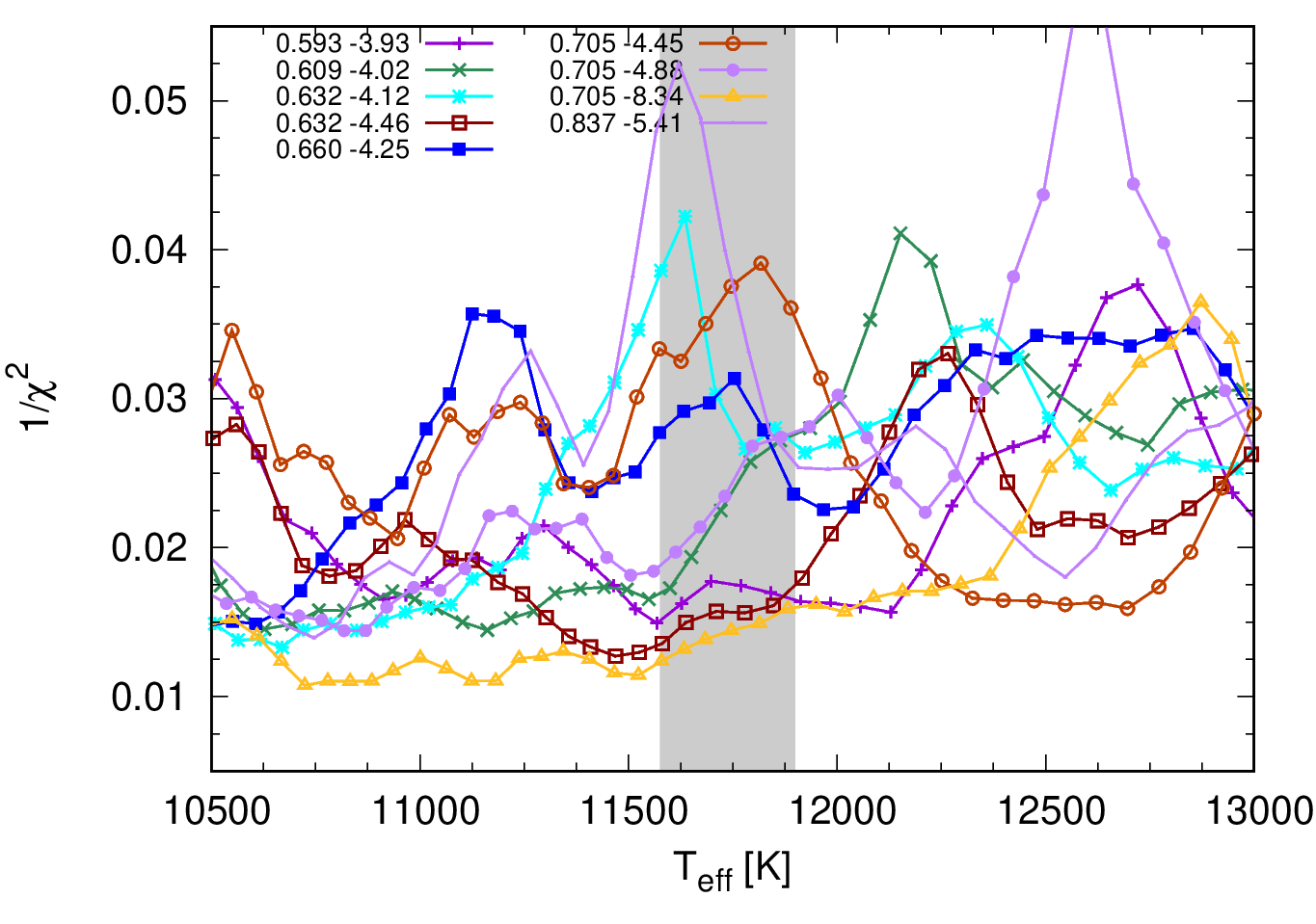
Figure 12: Inverse of the squared quality function $\chi$ in terms of the effective temperature for the best-fit models that agrees with Gaia distance within 10% (labeled here according to their respective $M_{\star}$, log$(M_{\rm H}/M_{\star})$ values). The grey region represents the averaged $T_{\rm eff}$ and its error from MWDD. For comparison, we also include the model that best matches the pulsation periods of G 29$-$38.

We assessed the internal uncertainties for the derived stellar mass, effective temperature, and surface gravity of the best-fit model by adopting the formula:

$$\sigma_{i}^{2}=\frac{d_{i}^{2}}{(S-S_{0})},$$ (5)

where $\sigma_{i}$ refers to the uncertainty in each quantity, $S_{0}\equiv\chi(M_{*}^{0},M_{H}^{0},T_{\rm eff}^{0})$ is the minimum of $\chi$, the quality function, and $S$ is the value of $\chi$ when the parameter $i$ is changed by $d_{i}$ while the other parameters remain fixed (Zhang et al., 1986; Castanheira & Kepler, 2008; Romero et al., 2012; Córsico et al., 2019b). The parameter $d_{i}$ can be interpreted as the step in the grid of the quantity $i$. From the uncertainties in $M_{\star}$ and $T_{\rm eff}$, we derived the uncertainties in $\log g$, $L_{\star}$ and $R_{\star}$. We found $\sigma_{M_{\star}}=0.03~{}M_{\odot}$, $\sigma_{T_{\rm eff}}=178$ K, $\sigma_{\log g}=0.05$, $\sigma_{L_{\star}/L_{\odot}}=2\times 10^{-4}$ and $\sigma_{R_{\star}/R_{\odot}}=1\times 10^{-4}$. These errors are formal uncertainties inherent to the process of searching for the asteroseismological model.

4.3 Asteroseismological distance

We can estimate the asteroseismic distance for G 29-38 based on the derived stellar parameters. From the effective temperature and gravity, we determined the absolute magnitude of our best-fit models in the Gaia $G$ band (Koester priv. comm.). For the 0.632 $M_{\odot}$ solution we find an absolute magnitude of $M_{\rm G}=11.839\pm 0.034$ mag. From the apparent magnitude obtained by Gaia Data Release 3 (DR3) Archive for G 29$-$38 ($m_{\rm G}=13.06$ mag), we obtain an asteroseismic distance of $d=17.54\pm 0.27$ pc, and parallax of $\pi=56.9\pm 1.$ mas. An important aspect of validating our asteroseismic best-fit model is by comparing the asteroseismic distance with that obtained directly by Gaia. We found an excellent agreement with the Gaia distance (Bailer-Jones et al., 2021), which reports of $d=17.51^{+0.008}_{-0.007}$ pc ($\pi=57.097_{-0.023}^{+0.025}$ mas). We repeated this process to each of the potential solutions.

4.4 Comparison with previous works

G 29$-$38 has been the subject of several detailed period-to-period fit analyses in the past decades, based on the pulsation periods found by Kleinman et al. (1998) and Thompson et al. (2008) (see Table 7 for a summary of the most important stellar parameters derived in each study).

The first detailed asteroseismic analysis for G 29$-$38 was done by Castanheira & Kepler (2009) based on the mean period values detected by Kleinman et al. (1998). These authors employed numerical models computed with the White Dwarf Evolutionary Code (WDEC, see Wood, 1990, and references therein) in which they considered $T_{\rm eff}$, $M_{\star}$, $M_{\rm H}$ and $M_{\rm He}$ as free parameters, but a fixed core composition of 50% ¹²C and 50% ¹⁶O. By assuming all the observed pulsation periods as $\ell=1$ modes, the authors found an asteroseismic model characterized by $T_{\rm eff}=11\,700$ K, $M_{\star}=0.665\,M_{\odot}$ with a thin H-envelope. The second asteroseismic analysis was performed by Romero et al. (2012) who adopted the same periods as in Castanheira & Kepler (2009) but their analysis was done adopting fully evolutionary models. The authors found a seismological solution for this star with $0.593\,M_{\odot}$, 11 471 K, and a very thin H-envelope of $4.67\times 10^{-10}M_{\star}$, with most observed pulsation periods fitted as $\ell=2$ modes, except the 614 s.

Finally, Chen & Li (2013) performed asteroseismological fits by adopting the period spectrum derived from Thompson et al. (2008) and models from WDEC. These models resemble those from Castanheira & Kepler (2009) but with a different (fixed) core composition. The authors derived two best-fit solutions fitted with a mix of $\ell=1,2$ modes and characterized by $T_{\rm eff}=11\,900$ K, $M_{\star}=0.790\,M_{\odot}$, $M_{\rm H}=10^{-4}M_{\star}$ and $T_{\rm eff}=11\,250$ K, $M_{\star}=0.780\,M_{\odot}$, $M_{\rm H}=3.16\times 10^{-6}M_{\star}$. Both solutions have nearly the same mass and log$g$, but they differ in $T_{\rm eff}$ and the hydrogen content.

We found good agreement with previous asteroseismic determinations for $T_{\rm eff}$, with maximum deviations of $\sim$ 3%. In particular, our derived $M_{\star}$ show better agreement with that from Castanheira & Kepler (2009) and Romero et al. (2012), with differences less than 7% and larger differences when comparing with the results from Chen & Li (2013) –up to 25%–. The comparison of other quantities such as the central abundance of C and O ($X_{\rm C}$, $X_{\rm O}$) or the thickness of the hydrogen envelope ($\log(1-M_{\rm H}/M_{\star})$) is more complex because of the different structures of the DA WD models and the different set of pulsation periods involved in each study.

Table 7: Stellar parameters from previous asteroseismological studies for G 29$-$38. K98* refers to the mean period values based on K98. $X_{\rm C}$ and $X_{\rm O}$ refer to the central abundance of carbon and oxygen, respectively.

	Dataset	$T_{\rm eff}$ (K)	$M_{\star}$ ($M_{\odot}$)	$\log g$	$M_{\rm H}/M_{\star}$	$M_{\rm He}/M_{\star}$	$\log(L/L_{\odot})$	$\log(R/R_{\odot})$	$X_{\rm C}$	$X_{\rm O}$
Castanheira & Kepler (2009)	K98*	11 700	0.665	…	1.0$\times 10^{-8}$	1.$\times 10^{-2}$	…	…	0.500	0.500
Romero et al. (2012)	K98*	11 471	0.593	8.01	4.6$\times 10^{-10}$	2.39$\times 10^{-2}$	-2.612	-1.901	0.283	0.704
Chen & Li (2013)	T08	11 900	0.790	8.30	1.0$\times 10^{-4}$	1.0$\times 10^{-2}$	…	…	0.200	0.800
		11 250	0.780	8.30	3.1$\times 10^{-6}$	3.1$\times 10^{-3}$	…	…	0.200	0.800
This work	K98+T98+TESS	11 635	0.632	8.04	7.58$\times 10^{-5}$	$1.74\times 10^{-2}$	-2.594	-1.905	0.232	0.755

4.5 Uncertainties from the progenitor evolution

Two primary approaches exist for conducting asteroseismic analysis of pulsating WD stars. One process involves constructing static stellar structures using parameterized luminosity and chemical profiles mildly based on stellar evolution outcomes (Bischoff-Kim & Østensen, 2011; Bischoff-Kim et al., 2014; Bischoff-Kim et al., 2019; Giammichele et al., 2014, 2016, 2017). While this method enables highly accurate fits, it may not fully align with current understanding of stellar evolution (Timmes et al., 2018; De Gerónimo et al., 2019) or with Gaia astrometry (Bell, 2022). The other approach, which is employed in this study, entails utilizing fully evolutionary models computed from the zero-age main sequence (ZAMS) to the ZZ Ceti stage (Althaus et al., 2010b; Romero et al., 2012). It is worth noting, however, that these models are subject to uncertainties in the modeling of physical processes inside the stars. Past research has demonstrated that asteroseismic analysis of ZZ Ceti stars using fully evolutionary models can lead to deviations of up to 8% in inferred values of $T_{\rm eff}$ and 5% in $M_{\star}$, as well as up to two orders of magnitude in the mass of the H envelope (De Gerónimo et al., 2017, 2018). These findings are primarily applicable to low-mass WDs, where uncertainties during prior evolution have a larger influence on the period spectrum of ZZ Ceti stars than in massive WDs ($\gtrsim 0.8M_{\odot}$, see De Gerónimo et al., 2017).

5 Summary and Conclusions

This work presents a detailed astroseismological study of G 29$-$38 based on short and ultra-short cadences TESS observations. G 29$-$38 was observed by TESS in two sectors, sector 42 and sector 56, totaling 51 days. Using the high-precision photometry data, we identified 28 significant frequencies from sector 42 and 38 significant frequencies from sector 56. The oscillation frequencies have periods from $\sim$260 s to $\sim$1400 s and are associated with $g$-mode pulsations. Additionally, we identified 30 combination frequencies per sector. Using the rotational frequency multiplets, we found four complete triplets and a quintuplet with a mean separation $\delta\nu_{\ell=1}$ = 4.67 $\mu$Hz and $\delta\nu_{\ell=2}$ = 6.67 $\mu$Hz, respectively, implying a rotation period of about 1.35 ($\pm 0.1$) days. This result is in line with what has been found by Hermes et al. (2017), who demonstrated that $0.51-0.73M_{\odot}$ white dwarfs evolved from $1.7-3.0M_{\odot}$ ZAMS progenitors, and have a mean rotation period of 1.46 d.

Based on the $\ell=1$ and $\ell=2$ modes defined by rotational triplets and quintuplets in conjunction with statistical tests, we searched for a constant period spacing for $\ell=1$ and $\ell=2$ modes. Using solely TESS observations, we identified 12 $\ell=1$ modes with radial order $k$ values ranging from 13 to 32 and 15 $\ell=2$ modes with $k$ values between 20 and 47 as presented in Table 3. We determined a constant period spacing of 41.20 s for $\ell=1$ modes and 22.58 s for $\ell=2$ modes, which are in good agreement with those inferred from the Kolmogorov-Smirnov, the inverse variance, and the Fourier transform statistical tests. We compared the constant period spacing obtained for the $\ell=1$ modes (41.20 s) with that from our numerical models. Due to the intrinsic degeneracy of the dependence of $\Delta\Pi$ with $M_{\star}$, $T_{\rm eff}$ and $M_{\rm H}$ we were able to derive only a range for the stellar mass for G 29$-$38 which is between $0.609\,M_{\odot}$ (with thick H envelope) and $0.877\,M_{\odot}$ (with thin H envelope). This analysis discards the existence of low-mass ($<0.609M_{\odot}$) solutions.

We combined the set of pulsation periods observed by TESS and those from previous works (Kleinman et al., 1998; Thompson et al., 2008) and derived a complete set of pulsation periods for G 29$-$38. We applied exhaustive asteroseismic period-to-period analysis and derived an asteroseismological model with stellar mass $M_{\star}/M_{\odot}=0.632\pm 0.03$, which is in good agreement with the value inferred from the period spacing analysis and also with the most recent spectroscopic determinations. Our results are in very good agreement with the asteroseismic results from Castanheira & Kepler (2009) and Romero et al. (2012), regarding the derived $T_{\rm eff}$ and $M_{\star}$. Finally, from the derived $T_{\rm eff}$ and $\log g$, we estimated the seismological distance of our best-fit model (17.54 pc) that is in excellent agreement with that provided directly by Gaia (17.51 pc).

Data Availability

Data from TESS is available at the MAST archive: https://mast.stsci.edu/search/hst/ui/$#$/.

Appendix A Full frequency list

Table 8: Detected frequencies, periods, and amplitudes (and their uncertainties) and the signal-to-noise ratio from the data of sector 42.

$\nu$	$\Pi$	$A$	S/N
($\mu$Hz)	(s)	(ppt)
1106.833 (17)	903.478 (14)	1.458 (10)	11.7
1115.196 (33)	896.712 (27)	0.900 (13)	7.5
1223.515 (27)	817.316 (18)	0.908 (10)	7.3
1231.161 (15)	812.241 (10)	1.662 (10)	13.3
1232.854 (11)	811.125 (77)	2.197 (10)	17.6
1292.603 (41)	773.646 (79)	4.240 (13)	35.3
1298.883 (02)	769.892 (14)	10.544 (10)	84.4
1307.303 (15)	764.942 (66)	2.627 (13)	21.9
1474.048 (07)	678.403 (35)	3.307 (10)	26.5
1526.590 (05)	655.054 (22)	4.983 (10)	39.9
1530.251 (05)	653.487 (23)	4.736 (10)	38.0
1633.792 (05)	612.073 (19)	5.018 (10)	40.2
1637.552 (05)	610.667 (19)	5.035 (10)	40.3
1642.383 (09)	608.871 (36)	2.640 (10)	21.1
1745.251 (18)	572.983 (62)	1.339 (10)	10.7
1750.641 (36)	571.219 (11)	0.696 (10)	5.6
1756.076 (09)	569.451 (29)	2.796 (10)	22.4
1836.735 (11)	544.444 (34)	2.186 (10)	17.5
1986.868 (11)	503.304 (26)	1.261 (13)	10.5
2001.060 (02)	499.735 (06)	9.904 (10)	79.2
2016.620 (26)	495.879 (63)	2.476 (11)	23.1
2110.152 (38)	473.899 (86)	0.655 (10)	5.2
2492.399 (04)	401.219 (08)	5.216 (10)	41.7
2497.176 (17)	400.452 (28)	1.455 (10)	11.7
2501.974 (18)	399.684 (29)	1.373 (10)	11.0
2747.582 (29)	363.956 (39)	0.845 (10)	6.8
3522.773 (07)	283.867 (06)	3.263 (10)	26.1
3639.341 (30)	274.775 (23)	0.822 (10)	6.6
1526.590 - 1298.883	227.829 (39)	4389.244 (76)	0.634 (10)	5.1
1633.792 - 1298.883	334.773 (31)	2987.092 (27)	0.809 (10)	6.5
4134.738 - 3790.969	344.944 (37)	2899.014 (31)	0.670 (10)	5.4
2001.060 - 1633.792	367.142 (31)	2723.741 (23)	0.812 (10)	6.5
2492.399 - 2001.060	491.278 (20)	2035.504 (85)	1.219 (10)	9.8
2001.060 - 1298.883	702.168 (12)	1424.159 (24)	2.103 (10)	16.8
2492.399 - 1633.792	858.687 (35)	1164.568 (47)	0.714 (10)	5.7
1986.868 - 1106.833	879.813 (38)	1136.605 (50)	0.650 (10)	5.2
2492.399 - 1298.883	1193.387 (26)	837.951 (18)	0.934 (10)	7.5
3522.773 - 1298.883	2223.717 (39)	449.697 (81)	0.631 (10)	5.1
2*1298.883	2598.084 (21)	384.898 (32)	1.178 (10)	9.4
1232.854 + 1530.251	2762.973 (29)	361.929 (39)	0.849 (10)	6.8
1298.883 + 1474.048	2772.942 (26)	360.627 (34)	0.965 (10)	7.7
1298.883 + 1526.590	2825.702 (25)	353.894 (32)	0.973 (10)	7.8
1292.603 + 1637.553	2930.010 (26)	341.295 (31)	0.957 (10)	7.7
1298.887 + 1637.552	2936.468 (29)	340.545 (35)	0.844 (10)	6.8
1298.887 + 1642.383	2941.162 (35)	340.001 (42)	0.702 (10)	5.6
1474.048 + 1526.590	3000.584 (36)	333.268 (40)	0.699 (10)	5.6
1298.883 + 1756.076	3054.962 (33)	327.336 (35)	0.760 (10)	6.1
1106.833 + 2001.060	3107.923 (19)	321.758 (21)	1.265 (10)	10.1
1530.251 + 1637.552	3167.776 (27)	315.678 (28)	0.908 (10)	7.3
1307.303 + 1986.868	3294.300 (27)	303.5546 (89)	0.94 (11)	8.8
1298.883 + 2001.060	3300.127 (19)	303.018 (18)	1.304 (10)	10.4
1474.048 + 2001.060	3475.100 (24)	287.761 (20)	1.046 (10)	8.4
1526.590 + 2001.060	3527.709 (29)	283.470 (24)	0.862 (10)	6.9
1530.251 + 2001.060	3531.294 (31)	283.182 (25)	0.799 (10)	6.4
1642.383 + 2001.060	3643.330 (36)	274.474 (27)	0.698 (10)	5.6
1298.883 + 2492.399	3790.969 (37)	263.784 (26)	0.679 (10)	5.4
2*2001.060	4002.150 (44)	249.865 (28)	0.571 (10)	4.6
1642.383 + 2492.399	4134.738 (40)	241.853 (23)	0.630 (10)	5.0

Table 9: Detected frequencies, periods, and amplitudes (and their uncertainties) and the signal-to-noise ratio from the data of sector 56.

$\nu$	$\Pi$	$A$	S/N
($\mu$Hz)	(s)	(ppt)
740.059 (21)	1351.244 (13)	0.742 (69)	6.9
838.89 (18)	1192.051 (12)	0.857 (69)	7.9
864.037 (19)	1157.358 (12)	0.801 (69)	7.4
1006.627 (19)	993.417 (11)	0.834 (69)	7.7
1012.964 (07)	987.202 (10)	2.268 (69)	21.0
1064.336 (13)	939.553 (11)	1.216 (69)	11.3
1111.944 (05)	899.326 (10)	11.84 (47)	109.8
1112.643 (05)	898.761 (10)	5.144 (74)	47.7
1151.511 (06)	868.424 (10)	2.801 (69)	26.0
1164.353 (04)	858.846 (10)	4.056 (69)	37.6
1181.656 (10)	846.270 (10)	1.49 (69)	13.8
1210.47 (02)	826.125 (10)	8.668 (69)	80.4
1225.755 (30)	815.824 (12)	1.085 (10)	10.1
1279.511 (17)	781.549 (11)	0.914 (69)	8.5
1371.426 (12)	729.168 (10)	1.315 (69)	12.2
1401.587 (18)	713.477 (10)	0.85 (69)	7.9
1431.995 (25)	698.327 (11)	0.612 (69)	5.7
1475.167 (10)	677.889 (10)	1.627 (69)	15.1
1481.34 (08)	675.065 (10)	1.906 (69)	17.7
1487.704 (14)	672.177 (10)	1.074 (69)	10.0
1522.859 (02)	656.660 (10)	9.462 (69)	87.7
1530.651 (03)	653.317 (10)	4.959 (69)	45.9
1539.918 (11)	649.385 (10)	1.467 (69)	13.6
1628.166 (01)	614.188 (10)	16.122 (69)	149.4
1649.424 (11)	606.272 (10)	1.346 (69)	12.5
1940.523 (15)	515.325 (10)	1.064 (69)	9.9
1992.310 (48)	501.930 (12)	0.687 (69)	6.3
1999.742 (02)	500.065 (10)	6.948 (69)	64.4
2006.51 (09)	498.378 (10)	1.811 (69)	16.8
2013.93 (12)	496.542 (10)	1.274 (69)	11.8
2045.91 (18)	488.780 (10)	0.853 (69)	7.9
2104.979 (27)	475.064 (62)	0.809 (99)	7.5
2223.76 (04)	449.689 (10)	3.499 (69)	32.4
2327.068 (18)	429.725 (10)	0.881 (69)	8.2
2492.19 (07)	401.254 (10)	2.37 (69)	22.0
2497.184 (15)	400.451 (10)	1.061 (69)	9.8
2502.278 (07)	399.636 (10)	2.345 (69)	21.7
2594.995 (21)	385.357 (10)	0.741 (69)	6.9
3754.433 (17)	266.352 (10)	0.893 (69)	8.3
1628.166 - 1522.859	105.262 (14)	9500.105 (1.26)	1.075 (69)	10.0
1522.859 - 1210.47	312.364 (11)	3201.393 (11)	1.361 (69)	12.6
1475.167 - 1111.944	363.789 (19)	2748.846 (14)	0.82 (69)	7.6
1530.651 - 1164.353	366.346 (18)	2729.660 (13)	0.886 (69)	8.2
1999.742 - 1628.166	371.551 (08)	2691.421 (15)	2.041 (69)	18.9
1628.166 - 1210.47	417.708 (05)	2394.017 (12)	3.247 (69)	30.1
1999.742 - 1522.859	476.841 (08)	2097.135 (13)	1.935 (69)	17.9
1628.166 - 1111.944	516.212 (18)	1937.189 (16)	0.866 (69)	8.0
371.551 + 417.708	789.277 (14)	1266.982 (12)	1.07 (69)	9.9
417.708 + 476.841	894.484 (21)	1117.963 (12)	0.729 (69)	6.8
838.89 + 894.484	1733.431 (23)	576.891 (10)	0.66 (69)	6.1
1111.944 + 1064.336	2176.203 (20)	459.516 (10)	0.776 (69)	7.2
1111.944 + 1210.47	2322.685 (15)	430.536 (10)	1.02 (69)	9.3
1111.944 + 1522.859	2634.85 (15)	379.528 (10)	1.06 (69)	9.8
1111.944 + 1530.651	2642.705 (11)	378.400 (10)	1.42 (69)	13.2
1111.944 + 1628.166	2740.103 (11)	364.950 (10)	1.455 (69)	13.5
1628.166 + 1210.47	2838.662 (10)	352.279 (10)	1.573 (69)	14.6
1522.859*2	3045.74 (23)	328.327 (10)	0.674 (69)	6.2
1111.944 + 1999.742	3111.529 (17)	321.385 (10)	0.918 (69)	8.5
312.364 + 2838.662	3151.02 (08)	317.358 (10)	1.956* (69)	18.1
1530.651 + 1628.166	3158.84 (21)	316.572 (10)	0.737 (69)	6.8
1628.166*2	3256.321 (12)	307.095 (10)	1.283 (69)	11.9
1111.944 + 2223.76	3335.497 (11)	299.805 (10)	1.36 (69)	12.6
1522.859 + 1999.742	3522.785 (08)	283.866 (10)	1.921 (69)	17.8
1628.166 + 1999.742	3627.914 (13)	275.641 (10)	1.214 (69)	11.3
1628.166 + 2223.76	3851.865 (18)	259.615 (10)	0.875 (69)	8.1
1628.166 + 2502.278	4130.428 (21)	242.106 (10)	0.722 (69)	6.7
2223.76*2	4447.332 (20)	224.854 (10)	0.76 (69)	7.0

References

- Aerts et al. (2010) Aerts C., Christensen-Dalsgaard J., Kurtz D. W., 2010, Asteroseismology
- Althaus et al. (2008) Althaus L. G., Córsico A. H., Kepler S. O., Miller Bertolami M. M., 2008, A&A, 478, 175
- Althaus et al. (2010a) Althaus L. G., Córsico A. H., Isern J., García-Berro E., 2010a, A&ARv, 18, 471
- Althaus et al. (2010b) Althaus L. G., Córsico A. H., Bischoff-Kim A., Romero A. D., Renedo I., García-Berro E., Miller Bertolami M. M., 2010b, ApJ, 717, 897
- Bailer-Jones et al. (2021) Bailer-Jones C. A. L., Rybizki J., Fouesneau M., Demleitner M., Andrae R., 2021, VizieR Online Data Catalog, p. I/352
- Bédard et al. (2017) Bédard A., Bergeron P., Fontaine G., 2017, ApJ, 848, 11
- Bell (2022) Bell K. J., 2022, Research Notes of the American Astronomical Society, 6, 244
- Bell et al. (2015) Bell K. J., Hermes J. J., Bischoff-Kim A., Moorhead S., Montgomery M. H., Østensen R., Castanheira B. G., Winget D. E., 2015, ApJ, 809, 14
- Bell et al. (2019) Bell K. J., et al., 2019, A&A, 632, A42
- Bischoff-Kim & Østensen (2011) Bischoff-Kim A., Østensen R. H., 2011, ApJ, 742, L16
- Bischoff-Kim et al. (2014) Bischoff-Kim A., Østensen R. H., Hermes J. J., Provencal J. L., 2014, ApJ, 794, 39
- Bischoff-Kim et al. (2019) Bischoff-Kim A., et al., 2019, ApJ, 871, 13
- Bognar & Sodor (2016) Bognar Z., Sodor A., 2016, Information Bulletin on Variable Stars, 6184, 1
- Bohm & Cassinelli (1971) Bohm K. H., Cassinelli J., 1971, A&A, 12, 21
- Borucki et al. (2010) Borucki W. J., et al., 2010, Science, 327, 977
- Bradley (2021) Bradley P. A., 2021, Frontiers in Astronomy and Space Sciences, 8, 229
- Bradley & Kleinman (1997) Bradley P., Kleinman S. J., 1997, in Isern J., Hernanz M., Garcia-Berro E., eds, Astrophysics and Space Science Library Vol. 214, White dwarfs. p. 445, doi:10.1007/978-94-011-5542-7_64
- Brickhill (1975) Brickhill A. J., 1975, MNRAS, 170, 405
- Brickhill (1991) Brickhill A. J., 1991, MNRAS, 251, 673