Timely Fusion of Surround Radar/Lidar for Object Detection in Autonomous Driving Systems

Abstract

Fusing Radar and Lidar sensor data can fully utilize their complementary advantages and provide more accurate reconstruction of the surrounding for autonomous driving systems. Surround Radar/Lidar can provide $360\mathrm{°}$ view sampling with the minimal cost, which are promising sensing hardware solutions for autonomous driving systems. However, due to the intrinsic physical constraints, the rotating speed of surround Radar, and thus the frequency to generate Radar data frames, is much lower than surround Lidar. Existing Radar/Lidar fusion methods have to work at the low frequency of surround Radar, which cannot meet the high responsiveness requirement of autonomous driving systems. This paper develops techniques to fuse surround Radar/Lidar with working frequency only limited by the faster surround Lidar instead of the slower surround Radar, based on the state-of-the-art object detection model MVDNet. The basic idea of our approach is simple: we let MVDNet work with temporally unaligned data from Radar/Lidar, so that fusion can take place at any time when a new Lidar data frame arrives, instead of waiting for the slow Radar data frame. However, directly applying MVDNet to temporally unaligned Radar/Lidar data greatly degrades its object detection accuracy. The key information revealed in this paper is that we can achieve high output frequency with little accuracy loss by enhancing the training procedure to explore the temporal redundancy in MVDNet so that it can tolerate the temporal unalignment of input data. We explore several different ways of training enhancement and compare them quantitatively with experiments.

I Introduction

Accurate perception of the surroundings is an essential function of autonomous driving systems (ADS). Lidar and Radar are two sought-after sensors for perception in ADS [1, 2, 3]. While Lidar sensors can generate fine-grained point clouds with rich information in good weather conditions, they fail in adverse weather (e.g., fog, snow) [4]. By contrast, Radar sensors are less impacted by adverse weather condition but less precise than Lidar [5]. Fusing Lidar and Radar data can overcome their individual weakness and yields more accurate object detection, which are promising solutions to provide accurate and robust perception capability for ADS [6, 7].

To provide a full view of the surrounding environment, the Lidar and Radar sensors on the vehicle need to cover the entire $360\mathrm{°}$ angle. One possible way to achieve this is to mount multiple sensors with different orientations, each covering a certain angle, and combine their data to construct a $360\mathrm{°}$ full view, but the overall cost of this approach is high. Alternatively, we can use surround Radar/Lidar to capture the $360\mathrm{°}$ full-view, which is more economic. The temporal resolution of surround Radar/Lidar, i.e., the frequency for them to produce a full-view data frame, is limited by the rotating speed. As millimeter-waves (used by Radar) travel much slower than light (used by Lidar), the maximum allowed rotating speeds of Radar are lower than Lidar under the same condition in other aspects. For example, the rotating speed of a popular surround Lidar, Velodyne HDL-32E, is $20$Hz ($20$ cycles per second) [8, 9], while the state-of-the-art surround Radar, NavTech CTS350-X, rotates with $4$Hz ($4$ cycles per second) [10, 11]. Therefore, we must properly handle the inconsistent input frequencies between the surround Radar and Lidar when fusing their data. A straightforward solution is to down-sample the Lidar data at the same frequency as the Radar. Some recent work combined several consecutive data frames of Lidar to produce one artificial Lidar data frame which matches the low frequency of Radar [4, 12, 13, 14]. In either way, fusion is performed with the rotating frequency of Radar. For example, with a surround Lidar with a rotating frequency $20$Hz and a surround Radar with a rotating frequency $4$Hz, fusion is performed and thus generates full-view reconstruction $4$ times per second. Typically, ADS requires to capture events and take proper reaction in a short time, e.g., $100$ms. Therefore, the low frequency of surround Radar/Lidar fusion makes it unsuitable for ADS from the real-time performance perspective.

In this paper, we develop techniques to address the above problem, i.e., to increase the frequency to perform Radar/Lidar fusion, so that it is not limited by the low rotating frequency of surround Radar. Our work is based on MVDNet, the state-of-the-art Radar/Lidar data fusion DNN model for object detection. The high-level idea of our approach is very simple: we can perform the fusion when a new Lidar data frame arrives, and let it fuse with the latest available Radar data frame which arrived at a slightly earlier point. However, by doing this, the temporal inconsistency of the Radar and Lidar sensor data will significantly degrade the detection accuracy. The key information revealed in this paper is that, by properly enhancing the training phase, we can actually make MVDNet tolerate the temporal inconsistency with tiny accuracy loss. We explored different ways to enhance the training procedure and evaluated them quantitatively through experiments.

II Related Work

To enhance 3D perception in autonomous driving, many works have proposed to fuse different sensor data modalities to leverage their complementary advantages, including cameras, Lidars, and Radars. MVDNet [4] proposes a fusion model to fuse Radar and Lidar with an attention mechanism for vehicle detection in foggy weather and achieves state-of-the-art results on the Oxford Radar RobotCar [15] (ORR) dataset. Li et al. [12] propose the ST-MVDNet to address the issue of missing sensor data in multi-modal vehicle detection for Radar/Lidar. Farag et al. [16] propose a Radar/Lidar data fusion method for real-time road-object detection and tracking for ADS. LiRaNet [14] is proposed for end-to-end trajectory prediction, which utilizes Radar sensor information along with Lidar and high-definition maps. Li et al. [17] develop EZFfusion framework for mutli-model 3D object detection and tracking based on camera, Lidar, and Radar. DEF[18] proposes a baseline fusion detector with all of the common sensors in ADS. FUTR3D [19] is a unified sensor fusion framework that can be used in almost any sensor configuration. However, existing Radar and Lidar fusion models are developed under the assumption that the Radar and Lidar data are perfectly synchronized. If not, downsampling the faster Lidar data at the same frequency as Radar is commonly used [4, 12, 13, 14, 16, 17, 18, 19]. From another perspective, some researchers in the real-time area develop the infrastructure-vehicle cooperative autonomous approaches to allow sensors to capture the environment in real-time and then perform timely fusion and perception [20, 21, 22, 23]. In this paper, we develop techniques to fuse temporally unaligned Radar/Lidar data and achieve high output frequency with little accuracy loss.

III Preliminary

We build our work based on MVDNet [4], the state-of-the-art Radar/Lidar fusion network. MVDNet fuses Radar intensity maps with Lidar point clouds, which harnesses their complementary capabilities. The architecture of MVDNet is shown in Fig. 1. MVDNet consists of two stages. The region proposal network (MVD-RPN) extracts feature maps from Lidar and Radar inputs and generates proposals. The region fusion network (MVD-RFN) pools and fuses region-wise features of the two sensors’ data frames and outputs oriented bounding boxes of detected vehicles.

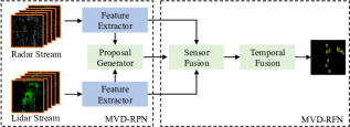
Figure 1: The architecture of MVDNet[4].

MVDNet assumes that the input Radar and Lidar frames have same timestamps. However, in the training data of MVDNet, the frequency of raw Radar frames, denoted by $F_{r}$, is different from the frequency of raw Lidar frames, denoted by $F_{l}$. MVDNet solves this problem by combining several consecutive raw Lidar frames into an artificial concatenated Lidar frame, which is generated with the same frequency as Radar data frames, as shown in Fig. 2. In this way, the fusion frequency of MVDNet equals $F_{r}$. We define

$$\emph{{ratio}}=\left\lfloor\frac{F_{l}}{F_{r}}\right\rfloor$$

and ratio+1+1 raw Lidar frames are aggregated to produce one concatenated Lidar data frame. More precisely, a subset of cloud points that covers $120\mathrm{°}$ view in each Lidar frame is selected, and these subsets are combined into a concatenated Lidar frame as shown in Fig. 2. Each concatenated Lidar frame and corresponding Radar frame are paired and sent to MVDNet.

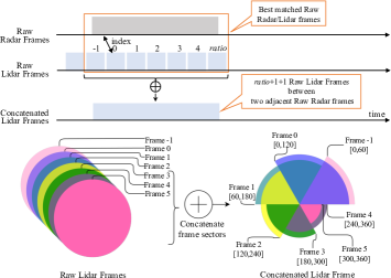
Figure 2: The Radar/Lidar frames alignment policy in MVDNet.

To improve accuracy, when fusing the latest paired Radar/Lidar frames, MVDNet uses historical frames. The number of historical frames is denoted by num_history. In MVDNet, num_history=4 by default. Decreasing num_history can reduce the computation workload of MVDNet inference, but at the cost of accuracy loss, as discussed in IV-D and IV-A.

IV The Proposed Method

IV-A Increasing the Radar/Lidar Fusion Frequency

Our method allows fusion to occur at any time when a raw Lidar frame arrives, instead of waiting for the slow Radar frames, so fusion can be triggered with a higher frequency, as long as the period of fusion is an integral multiple of the period of Lidar frames. The fusion frequency of our method is denoted by $F_{f}$. We define

$$\alpha=\frac{F_{l}}{F_{f}}$$ (1)

which should satisfy:

$$\alpha\in\{1,2,3,...,ratio\}$$ (2)

If $\alpha>\emph{{ratio}}$, the fusion between the paired Radar/Lidar frames will be meaningless because they have no overlap in time. Thus, $F_{f}$ should satisfy:

$$F_{r}\leq F_{f}\leq F_{l}$$ (3)

The fusion frequency is only limited by the faster Lidar instead of the slower Radar.

Fig. 3 shows two examples to demonstrate our fusion method. For the newly arrived raw Lidar frame, if the raw Radar frame in the same period has not arrived, the latest available raw Radar frame will be used for fusion. In Fig. 3(a), we assume that we expect to achieve a high fusion frequency $F_{f}=F_{l}$. According to Equation (1), we need to set $\alpha$=1, which means to perform timely fusion when each new raw Lidar frame arrives. In Fig. 3(a), the latest raw Radar frame has not been generated at $t_{8}^{l}$ and $t_{9}^{l}$. We perform the fusion between the latest concatenated Lidar frames (the orange box) and the latest available raw Radar frame (the orange box) generated at $t_{1}^{r}$ respectively. Fig. 3(b) shows another example with fusion frequency $F_{f}=F_{l}/3$. The fusion should be performed every 3 raw Lidar frame arrivals. Our method not only increases the fusion frequency, but also allows us to adjust the frequency according to the actual situation. In practice, the fusion results do not always have to be generated at the highest frequency. Based on the current vehicle speed and overall workload of the vehicle, the ADS is expected to provide a fusion frequency that can be adjusted.

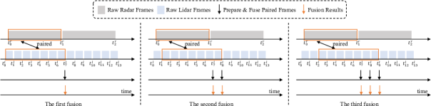
(a) The first example, $\alpha$=1,$F_{f}$=$F_{l}$.

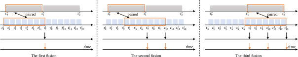
(b) The second example, $\alpha$=3,$F_{f}$=$F_{l}$/3.

Figure 3: Our proposed fusion method.

IV-B Training Enhancement to Maintain Accuracy

However, by directly applying the above method, the input Radar/Lidar frames to MVDNet are temporally unaligned, which greatly degrades the object detection accuracy. In fact, there is a time offset between each pair of unaligned Radar/Lidar frames, as shown in Fig. 4. We use offset to represent the number of complete raw Lidar frames that are ahead of Radar for each paired Radar/Lidar frames. The offset should satisfy:

$$\emph{{offset}}\in\{0,1,2,...,\emph{{ratio}}\}$$ (4)

For the same reason, if offset exceeds ratio, the fusion between paired Radar/Lidar frames will be meaningless because they are not overlapped in time.

Following MVDNet, we evaluate original MVDNet model to unaligned Radar/Lidar frames based on ORR dataset ($F_{l}=20$Hz, $F_{r}=4$Hz, ratio=5) using average precision (AP) in COCO evaluation [24] with Intersection-over-Union (IoU) of $0.5$, $0.65$, and $0.8$ for a fair comparison. For various offset settings, the accuracy result is shown in Table I. We observe that applying the original MVDNet model to unaligned Radar/Lidar frames greatly degrades object detection accuracy. The accuracy of the MVDNet model with unaligned frames (offset = $\{1,2,3,4,5\}$) is much lower than that with aligned frames (offset=0). Therefore, offset is a critical factor for accuracy.

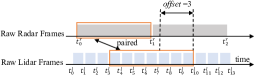
Figure 4: Offset between temporally unaligned frames.

TABLE I: Overall Performance of Directly Applying MVDNet on Radar/Lidar Frames:
AP of Oriented Bounding Boxes in Bird’s Eye View (BEV).

	offset	0			1			2			3			4			5
Model	IoU	0.5	0.65	0.8	0.5	0.65	0.8	0.5	0.65	0.8	0.5	0.65	0.8	0.5	0.65	0.8	0.5	0.65	0.8
MVDNet		0.897	0.877	0.735	0.652	0.619	0.486	0.616	0.587	0.462	0.583	0.559	0.441	0.51	0.498	0.411	0.521	0.508	0.407

To mitigate the above accuracy loss problem, we use the property of MVDNet that uses both the current pair and num_history (num_history=4) historical pairs, and a total of 1+num_history paired Radar/Lidar frames as the input for each fusion. There exists redundant information between continuous Radar/Lidar frames. We exploit the redundant information to make MVDNet still work well with temporally unaligned Radar/Lidar frames. We discover a simple but effective training enhancement method, which almost enables MVDNet to maintain accuracy when fusing temporally unaligned Radar/Lidar frames. For Radar/Lidar frames with different offset, we synthesize paired Radar/Lidar frames with corresponding offset to train MVDNet model from scratch.

Under the same experimental setting, the results of our method are summarized in Table II. The MVDNet_offset means that the MVDNet model is trained on the Radar/Lidar frames with a specific offset, offset$\in\{1,2,3,4,5\}$. For the unaligned Radar/Lidar frames with a specific offset, the MVDNet model trained on corresponding paired Radar/Lidar frames outperforms these MVDNet models trained on other offset frames. Comparing Table II and Table I, the accuracy of our enhancement training method on unaligned Radar/Lidar frames with each specific offset is almost equal to the original MVDNet model on aligned Radar/Lidar frames (offset=0). The results demonstrate that, on the premise of increasing the fusion frequency, our proposed fusion method maintains accuracy even when the Radar/Lidar frames are time unaligned.

TABLE II: Overall Performance of Our Fusion Method on Radar/Lidar frames: AP of Oriented Bounding Boxes in BEV.

Model	offset	1			2			3			4			5
	IoU	0.5	0.65	0.8	0.5	0.65	0.8	0.5	0.65	0.8	0.5	0.65	0.8	0.5	0.65	0.8
MVDNet_1		0.898	0.869	0.722	0.867	0.841	0.668	0.847	0.827	0.652	0.828	0.809	0.643	0.826	0.801	0.644
MVDNet_2		0.87	0.85	0.67	0.899	0.877	0.724	0.889	0.863	0.684	0.876	0.848	0.705	0.868	0.847	0.702
MVDNet_3		0.867	0.846	0.699	0.868	0.847	0.701	0.89	0.867	0.722	0.879	0.858	0.709	0.878	0.849	0.7
MVDNet_4		0.877	0.855	0.686	0.881	0.853	0.683	0.874	0.853	0.688	0.888	0.86	0.709	0.875	0.854	0.688
MVDNet_5		0.855	0.833	0.679	0.862	0.834	0.687	0.865	0.843	0.689	0.884	0.864	0.704	0.885	0.865	0.707

IV-C Exploiting Different Enhancement Strategies

In order to enable MVDNet model to deal with Radar/Lidar frames with various offset, we exploit two different enhancement strategies.

Separate training strategy. For temporally unaligned Radar/Lidar frames with different offset, the first strategy is to train a corresponding MVDNet model separately for each offset frame. During training, we firstly train a shared MVDNet model based on the paired Radar/Lidar frames with offset=$\lceil\emph{{ratio}}/2\rceil$, and share the parameter weights of its MVD-RPN among other MVDNet models which deal with different offset frames. Secondly, MVD-RFN of each MVDNet model is fine-tuned based on corresponding offset frames. We can obtain multiple MVDNet models and each model deals with the Radar/Lidar frames with a specific offset. The evaluation results based on ORR dataset are summarized in Table III. The MVDNet_separated_offset means that the MVDNet model is fine-tuned on the Radar/Lidar frames offset, offset$\in${0,1,2,…,5}. We observe that for the Radar/Lidar frames with a specific offset, each MVDNet_separated_offset model fine-tuned on corresponding offset frames can get the best accuracy performance compared with other models.

TABLE III: Overall performance of separately trained MVDNet models : AP of oriented bounding boxes in BEV.

Model	offset	0			1			2			3			4			5
	IoU	0.5	0.65	0.8	0.5	0.65	0.8	0.5	0.65	0.8	0.5	0.65	0.8	0.5	0.65	0.8	0.5	0.65	0.8
MVDNet_separated_0		0.899	0.878	0.736	0.848	0.826	0.679	0.838	0.817	0.675	0.83	0.809	0.68	0.802	0.79	0.671	0.803	0.792	0.663
MVDNet_separated_1		0.887	0.866	0.719	0.887	0.866	0.722	0.884	0.864	0.722	0.884	0.856	0.722	0.876	0.855	0.711	0.874	0.847	0.711
MVDNet_separated_2		0.867	0.846	0.708	0.876	0.856	0.656	0.886	0.865	0.722	0.883	0.856	0.722	0.874	0.855	0.718	0.867	0.854	0.712
MVDNet_separated_3		0.861	0.84	0.689	0.868	0.848	0.699	0.877	0.856	0.71	0.888	0.868	0.723	0.88	0.859	0.714	0.879	0.859	0.713
MVDNet_separated_4		0.841	0.82	0.682	0.848	0.828	0.694	0.858	0.838	0.703	0.878	0.859	0.725	0.887	0.868	0.725	0.879	0.86	0.723
MVDNet_separated_5		0.869	0.848	0.702	0.867	0.847	0.699	0.875	0.855	0.701	0.885	0.865	0.711	0.887	0.867	0.711	0.887	0.867	0.712

Mixed training strategy. The second strategy is to mix the same amount of paired Radar/Lidar frames with various offset together. During training, we use the new mixed training set to train a MVDNet_mixed model from scratch. We expect to obtain a MVDNet_mixed model that can handle Radar/Lidar frames with different offset. The evaluation results are summarized in Table IV. We observe that, for Radar/Lidar frames with different offset, the MVDNet_mixed model can achieve similar and good accuracy performance with different IoU settings.

TABLE IV: Overall Performance of The Mixed Training MVDNet Model: AP of Oriented Bounding Boxes in BEV.

Model	offset	0			1			2			3			4			5
	IoU	0.5	0.65	0.8	0.5	0.65	0.8	0.5	0.65	0.8	0.5	0.65	0.8	0.5	0.65	0.8	0.5	0.65	0.8
MVDNet_mixed		0.897	0.877	0.735	0.896	0.876	0.734	0.896	0.877	0.734	0.895	0.875	0.733	0.895	0.876	0.727	0.895	0.875	0.726

Comparing the results of the above two strategies, we observe two phenomena. First, for the aligned Radar/Lidar frames (offset=0), the separately fine-tuned MVDNet_separate_0 model achieves slightly better accuracy than the MVDNet_mixed model. Second, for other unaligned Radar/Lidar frames (offset$\in${1,2,3,4,5}), the MVDNet_mixed model achieves better accuracy than separately fine-tuned MVDNet_separated_1/2/3/4/5 models. Therefore, how to design a unified MVDNet model for various Radar/Lidar frames is a trade-off.

For separated training strategy, we design a multi-branch unified MVDNet as shown in Fig. 5. The unified MVDNet consists of three modules. The first module is feature extractors for Radar/Lidar frames. Due to the property that the lower layer of the neural network extracts low-level features [25], the low-level feature extractors can be used as the shared feature extractors for Radar/Lidar frames with different offset. The second fusion module has multiple branches, and each branch is used to fuse Radar/Lidar frames with a specific offset. The third module is a new input offset, which is used to determine which branch should be chosen for inference.

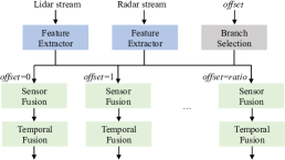
Figure 5: Structure of the multi-branch unified MDVNet.

IV-D Impact of Historical Information

In order to navigate the trade-off between latency and performance, we exploit two historical frame selection and matching strategies, which aim to reduce inference latency.

Historical frame skipping strategy. In the basic fusion method (Fig. 3), the current and historical paired Radar/Lidar frames are time consecutive. As shown in Fig. 6(a), if the num_history=2, the current and two consecutive paired Radar/Lidar frames are selected as the input frames. Considering the redundant information between successive Radar/Lidar frames, we explore a frame skipping method, which can use fewer frames to represent the same amount of information as the basic fusion method. Fig. 6(b) shows our frame skipping method with the same num_history=2 configuration, we select historical paired Radar/Lidar frames every two intervals, which will skip several frames. Each input frames only contain 3 paired Radar/Lidar frames, but the amount of information that can be represented is the same as that of the num_history=4 configuration. We expect our strategy can provide a new way for an accuracy-latency trade-off.

Table V shows the evaluation results. For the Radar/Lidar frames with a specific offset, offset$\in${0,1,2,…,5}, we observe that with the same num_history=2 configuration, our frame skipping method achieves similar or even better accuracy results than the method without frame skipping. Compared to the num_history=4 configuration, our method with num_history=2 configuration has only a slight loss of accuracy. Therefore, by skipping frames, our method reduces latency with little loss of accuracy.

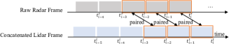
(a) The basic method, num_history=2.

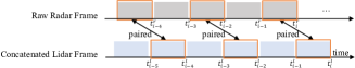
(b) Our frame skipping method, num_history=2.

Figure 6: Historical frame selection strategy.

TABLE V: Overall performance of frame skipping method: AP of oriented bounding boxes in BEV.

	offset	0			1			2			3			4			5
Strategy	IoU	0.5	0.65	0.8	0.5	0.65	0.8	0.5	0.65	0.8	0.5	0.65	0.8	0.5	0.65	0.8	0.5	0.65	0.8
Without frame skipping, num_history=4		0.897	0.877	0.735	0.898	0.869	0.722	0.899	0.877	0.724	0.89	0.867	0.722	0.888	0.86	0.709	0.885	0.865	0.707
Without frame skipping, num_history=2		0.871	0.85	0.725	0.883	0.863	0.72	0.885	0.866	0.721	0.885	0.864	0.718	0.869	0.856	0.712	0.878	0.866	0.723
With frame skipping, num_history=2		0.895	0.877	0.724	0.885	0.865	0.715	0.873	0.852	0.696	0.887	0.856	0.721	0.887	0.857	0.7	0.885	0.864	0.706

Historical frame alignment strategy. In the basic fusion method (Fig. 3), for each 1+num_history paired Radar/Lidar frames, if the current paired Radar/Lidar frames are misaligned, all the other historical paired frames are misaligned and exist the same offset. However, we observe that apart from the current paired frames, other historical concatenated Lidar frames can find their aligned Radar frames. As shown in Fig. 7, for the current concatenated Lidar frame at $t_{i}^{l}$, it can only pair with the latest available raw Radar frame that arrives at $t_{i}^{r}$. But for each historical concatenated Lidar frame, a new re-concatenated Radar frame that is aligned perfectly with the Lidar frame can be reconstructed based on two original adjacent raw Radar frames. Based on the observation, we exploit historical frame alignment strategy to align all historical paired Radar/Lidar frames in time. The basic idea is, when selecting each historical paired frame, reconstructing a new Radar frame that aligns with the concatenated Lidar frame according to the Lidar timestamp.

Table VI compares our historical frame alignment strategy with basic method. For the temporally unaligned Radar/Lidar frames with a specific offset, offset$\in${1,2,…,5}, we observe that our alignment strategy has no gain in accuracy.

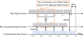
Figure 7: Historical frame alignment strategy, num_history=4.

TABLE VI: Overall performance of historical frame alignment strategy: AP of oriented bounding boxes in BEV.

	offset	1			2			3			4			5
Strategy	IoU	0.5	0.65	0.8	0.5	0.65	0.8	0.5	0.65	0.8	0.5	0.65	0.8	0.5	0.65	0.8
unaligned		0.898	0.869	0.722	0.899	0.877	0.724	0.89	0.867	0.722	0.888	0.86	0.709	0.885	0.865	0.707
aligned		0.889	0.859	0.694	0.895	0.874	0.732	0.88	0.859	0.718	0.879	0.859	0.705	0.856	0.836	0.687

V Conclusion

In this paper, we develop techniques to fuse surround Radar/Lidar with working frequency only limited by the faster surround Lidar instead of the slower surround Radar, based on the state-of-the-art Radar/Lidar fusion-based object detection model MVDNet. As far as possible, the advantages of the fast sampling of Lidar are played out, and a timely fusion is performed in temporally unaligned Radar/Lidar frames to provide real-time road condition information. The experiment results demonstrate that our proposed fusion method can increase the fusion frequency between temporally unaligned Radar/Lidar data with almost no loss of object detection accuracy.

References

- [1] Y. Li and J. Ibanez-Guzman, “Lidar for autonomous driving: The principles, challenges, and trends for automotive lidar and perception systems,” IEEE Signal Processing Magazine, vol. 37, no. 4, pp. 50–61, 2020.
- [2] T. Zhou, M. Yang, K. Jiang, H. Wong, and D. Yang, “Mmw radar-based technologies in autonomous driving: A review,” Sensors, vol. 20, no. 24, p. 7283, 2020.
- [3] Q. Zhang, H. Sun, Z. Wei, and Z. Feng, “Sensing and communication integrated system for autonomous driving vehicles,” in IEEE INFOCOM 2020-IEEE Conference on Computer Communications Workshops (INFOCOM WKSHPS). IEEE, 2020, pp. 1278–1279.
- [4] K. Qian, S. Zhu, X. Zhang, and L. E. Li, “Robust multimodal vehicle detection in foggy weather using complementary lidar and radar signals,” in Proceedings of the IEEE/CVF Conference on Computer Vision and Pattern Recognition, 2021, pp. 444–453.
- [5] S. Campbell, N. O’Mahony, L. Krpalcova, D. Riordan, J. Walsh, A. Murphy, and C. Ryan, “Sensor technology in autonomous vehicles: A review,” in 2018 29th Irish Signals and Systems Conference (ISSC). IEEE, 2018, pp. 1–4.
- [6] J. Kocić, N. Jovičić, and V. Drndarević, “Sensors and sensor fusion in autonomous vehicles,” in 2018 26th Telecommunications Forum (TELFOR). IEEE, 2018, pp. 420–425.
- [7] Z. Wang, Y. Wu, and Q. Niu, “Multi-sensor fusion in automated driving: A survey,” Ieee Access, vol. 8, pp. 2847–2868, 2019.
- [8] Velodyne hdl-32e lidar. [Online]. Available: https://velodynelidar.com/products/hdl-32e/
- [9] C. Kelly, B. Wilkinson, A. Abd-Elrahman, O. Cordero, and H. A. Lassiter, “Accuracy assessment of low-cost lidar scanners: An analysis of the velodyne hdl–32e and livox mid–40’s temporal stability,” Remote Sensing, vol. 14, no. 17, p. 4220, 2022.
- [10] Navtech cts350-x radar. [Online]. Available: https://navtechradar.com/?s=CTS350-X
- [11] M. Sheeny, E. De Pellegrin, S. Mukherjee, A. Ahrabian, S. Wang, and A. Wallace, “Radiate: A radar dataset for automotive perception in bad weather,” in 2021 IEEE International Conference on Robotics and Automation (ICRA). IEEE, 2021, pp. 1–7.
- [12] Y.-J. Li, J. Park, M. O’Toole, and K. Kitani, “Modality-agnostic learning for radar-lidar fusion in vehicle detection,” in Proceedings of the IEEE/CVF Conference on Computer Vision and Pattern Recognition, 2022, pp. 918–927.
- [13] J. Kim, Y. Kim, and D. Kum, “Low-level sensor fusion for 3d vehicle detection using radar range-azimuth heatmap and monocular image,” in Asian Conference on Computer Vision. Springer, 2020, pp. 388–402.
- [14] M. Shah, Z. Huang, A. Laddha, M. Langford, B. Barber, S. Zhang, C. Vallespi-Gonzalez, and R. Urtasun, “Liranet: End-to-end trajectory prediction using spatio-temporal radar fusion,” arXiv preprint arXiv:2010.00731, 2020.
- [15] D. Barnes, M. Gadd, P. Murcutt, P. Newman, and I. Posner, “The oxford radar robotcar dataset: A radar extension to the oxford robotcar dataset,” in 2020 IEEE International Conference on Robotics and Automation (ICRA). IEEE, 2020, pp. 6433–6438.
- [16] W. Farag, “Real-time lidar and radar fusion for road-objects detection and tracking,” International Journal of Computational Science and Engineering, vol. 24, no. 5, pp. 517–529, 2021.
- [17] Y. Li, J. Deng, Y. Zhang, J. Ji, H. Li, and Y. Zhang, “Ezfusion: A close look at the integration of lidar, millimeter-wave radar, and camera for accurate 3d object detection and tracking,” IEEE Robotics and Automation Letters, vol. 7, no. 4, pp. 11 182–11 189, 2022.
- [18] M. Bijelic, T. Gruber, F. Mannan, F. Kraus, W. Ritter, K. Dietmayer, and F. Heide, “Seeing through fog without seeing fog: Deep multimodal sensor fusion in unseen adverse weather,” in Proceedings of the IEEE/CVF Conference on Computer Vision and Pattern Recognition, 2020, pp. 11 682–11 692.
- [19] X. Chen, T. Zhang, Y. Wang, Y. Wang, and H. Zhao, “Futr3d: A unified sensor fusion framework for 3d detection,” arXiv preprint arXiv:2203.10642, 2022.
- [20] S. Liu, B. Yu, J. Tang, and Q. Zhu, “Towards fully intelligent transportation through infrastructure-vehicle cooperative autonomous driving: Challenges and opportunities,” in 2021 58th ACM/IEEE Design Automation Conference (DAC). IEEE, 2021, pp. 1323–1326.
- [21] A. Prakash, K. Chitta, and A. Geiger, “Multi-modal fusion transformer for end-to-end autonomous driving,” in Proceedings of the IEEE/CVF Conference on Computer Vision and Pattern Recognition, 2021, pp. 7077–7087.
- [22] J. Cui, H. Qiu, D. Chen, P. Stone, and Y. Zhu, “Coopernaut: End-to-end driving with cooperative perception for networked vehicles,” in Proceedings of the IEEE/CVF Conference on Computer Vision and Pattern Recognition, 2022, pp. 17 252–17 262.
- [23] Y. He, L. Ma, Z. Jiang, Y. Tang, and G. Xing, “Vi-eye: semantic-based 3d point cloud registration for infrastructure-assisted autonomous driving,” in Proceedings of the 27th Annual International Conference on Mobile Computing and Networking, 2021, pp. 573–586.
- [24] T.-Y. Lin, M. Maire, S. Belongie, J. Hays, P. Perona, D. Ramanan, P. Dollár, and C. L. Zitnick, “Microsoft coco: Common objects in context,” in European conference on computer vision. Springer, 2014, pp. 740–755.
- [25] A. Søgaard and Y. Goldberg, “Deep multi-task learning with low level tasks supervised at lower layers,” in Proceedings of the 54th Annual Meeting of the Association for Computational Linguistics (Volume 2: Short Papers), 2016, pp. 231–235.