Benne: A Modular and Self-Optimizing Algorithm for Data Stream Clustering

Abstract

In various real-world applications, ranging from the Internet of Things (IoT) to social media and financial systems, data stream clustering is a critical operation. This paper introduces Benne, a modular and highly configurable data stream clustering algorithm designed to offer a nuanced balance between clustering accuracy and computational efficiency. Benne distinguishes itself by clearly demarcating four pivotal design dimensions: the summarizing data structure, the window model for handling data temporality, the outlier detection mechanism, and the refinement strategy for improving cluster quality. This clear separation not only facilitates a granular understanding of the impact of each design choice on the algorithm’s performance but also enhances the algorithm’s adaptability to a wide array of application contexts. We provide a comprehensive analysis of these design dimensions, elucidating the challenges and opportunities inherent to each. Furthermore, we conduct a rigorous performance evaluation of Benne, employing diverse configurations and benchmarking it against existing state-of-the-art data stream clustering algorithms. Our empirical results substantiate that Benne either matches or surpasses competing algorithms in terms of clustering accuracy, processing throughput, and adaptability to varying data stream characteristics. This establishes Benne as a valuable asset for both practitioners and researchers in the field of data stream mining.

1 Introduction

Data Stream Clustering (DSC) serves as a cornerstone in the field of data stream mining, finding extensive applications across diverse real-world contexts including network intrusion detection [1], social network analysis [2], weather forecasting [3], and financial market analysis [4]. Unlike traditional batch clustering algorithms such as KMeans [5, 6] and DBSCAN [7], DSC algorithms dynamically group incoming data tuples based on attribute similarities. These algorithms are specifically designed to manage unique data stream challenges, notably cluster evolution and outlier evolution [2, 8, 9, 10, 11]. These terms refer to the shifting nature of data distributions and the emergence of new outliers over time.

In addition, DSC algorithms must grapple with the imperative of processing efficiency [12, 13]. They are often deployed in environments where time is of the essence, data streams at high velocities, and real-time decision-making is crucial. To balance the need for high clustering accuracy with constraints on computational resources, memory, and latency, various strategies have been investigated. These include incremental updates, data summarization, sketching techniques, and both online and offline processing methods. The relentless growth in the volume, velocity, and variety of data streams continues to pose both challenges and opportunities, keeping the design, optimization, and evaluation of DSC algorithms an area of active and pertinent research [14, 15, 2, 12, 13].

The multifaceted nature of use cases and the diversity in performance metrics have spurred the creation of a wide array of DSC algorithms [14, 16, 2, 17, 18, 15, 19, 20, 21, 17, 22, 23]. These algorithms are built on varying principles, methods, and heuristics, each tailored to meet specific needs in terms of application requirements, data characteristics, or performance objectives. For example, some algorithms are optimized for processing speed [15], making them ideal for high-velocity data streams. Others prioritize clustering accuracy [20, 14], a critical factor in applications requiring precise cluster assignments. Consequently, the task of selecting an appropriate DSC algorithm for real-world, diverse workloads becomes a complex endeavour. This complexity is exacerbated by the interdependent nature of several fundamental design choices in DSC algorithms, each with its own set of trade-offs and performance implications.

In a prior study [24], we rigorously examined four cornerstone design elements in data stream clustering (DSC) algorithms: data structure summarization, window modelling, outlier detection mechanisms, and refinement strategies. This comprehensive analysis led to the creation of Benne, a modular DSC algorithm. The modularity of Benne allows for effortless customization, making it adaptable to a variety of application domains. Whether the focus is on clustering accuracy, processing efficiency, or resilience to noise and outliers, Benne can be tailored to meet these specific performance goals.

In this work, we extend our investigation into Benne, elaborating on its modular architecture. We introduce three key enhancements to its design:

• First, we implement a ‘Regular Stream Characteristics Detection’ mechanism that routinely identifies dynamic changes in stream characteristics, such as cluster and outlier evolution, as well as shifts in workload dimensions.

• Second, we add an ‘Automatic Design Choice Selection’ feature, enabling Benne to adapt its component choices autonomously in response to changes in stream characteristics.

• Lastly, we introduce ‘Flexible Algorithm Migration,’ a feature designed to minimize clustering information loss during modular adjustments. This is achieved by transferring existing clustering results to the new configuration.

These enhancements, working in concert, equip Benne with the robustness needed to maintain stable performance across diverse optimization targets, even in the face of evolving stream characteristics.

We undertake a rigorous evaluation of Benne’s performance, comparing it with leading DSC algorithms across a variety of configurations. Our evaluation encompasses a broad spectrum of real-world and synthetic workloads, each with its unique set of characteristics. This comprehensive approach ensures the generalizability of our findings. Notably, Benne demonstrates superior performance in both purity and throughput metrics, excelling especially in scenarios characterized by high dimensionality and frequent cluster evolution. To make it readily accessible for both academic research and practical applications, we have also encapsulated Benne into a Python library. The source code for Benne is publicly available at https://github.com/intellistream/Sesame.

The structure of the remainder of this paper is as follows: Section 2 provides an overview of data stream characteristics, clustering objectives, and essential components of DSC algorithms. Section 3 details the modular design of DSC and its key components. Section 4 discusses the complete algorithmic design of Benne, including its automatic option selection mechanism. Section 5 presents our empirical evaluation of Benne and its automatic option selection mechanisms. Finally, Section 6 reviews additional related work, and Section 7 concludes the paper.

2 Preliminaries and Background

In this section, we discuss the data stream characteristics, clustering objectives, and essential components of DSC algorithms.

2.1 Foundational Concepts and Notations

In this subsection, we introduce key terms, notations, and essential components foundational to the understanding of DSC algorithms.

In mathematical terms, a data stream is represented as a sequence of tuples, denoted as $S=(x_{1},x_{2},\ldots,x_{t},\ldots)$, where $x_{t}$ denotes the $t$-th data point arriving at time $t$. Let $x_{t}$ be a data point in the stream, and $D(x_{t},C_{t})$ be the distance from $x_{t}$ to its closest cluster in $C_{t}$. If $D(x_{t},C_{t})>\delta$, where $\delta$ is a threshold, $x_{t}$ can be considered an outlier. DSC algorithms efficiently update $C_{t}$ to $C_{t+1}$ in response to changes in data distribution.

To measure the clustering quality of DSC algorithms, in this paper, we apply the most widely used metric, purity [25], which assesses how well the data points within each cluster belong to the same class. We also uses CMM [26], which is specifically designed for measuring DSC algorithms ability to handle the evolving activities in the stream. To evaluate the performance of the DSC algorithms, we introduce the throughput metric, which represents the amount of data that the algorithm can process within a certain period of time.

DSC algorithms typically consist of several key components to address the challenges posed by data streams: 1) Summarizing Data Structure provides a compact representation of data points, capturing essential information while minimizing memory usage, as storing the entire data stream is impractical. 2) Window Model handles the temporal aspect of data streams, focusing on recent data points and discarding outdated information, improving the algorithm’s clustering capability. 3) Outlier Detection Mechanism identifies and handles noise and outliers in the data stream, preventing them from affecting the clustering quality. Detecting outliers in data streams is a challenging task for DSC algorithms, particularly when outlier evolution occurs. 4) Refinement Strategy updates and refines the clustering model as new data points arrive, adapting to changes in the data distribution. This strategy usually applies once before getting the final clustering result, not significantly influencing efficiency but potentially improving accuracy.

2.2 Challenges and Objectives

Data streams introduce unique challenges for data mining algorithms due to their continuous, high-speed, and potentially infinite nature. As such, designing effective algorithms to cluster data streams requires a deep understanding of these challenges and clear objectives to guide the development.

2.2.1 Challenges

The challenges inherent to data stream clustering can be encapsulated in the four V’s:

Volume: Data streams can generate volumes of data that may surpass the system’s storage and processing limits. Efficient data summarization techniques are crucial for managing this challenge [27, 28]. Specifically, methods like sketching [29] have been incorporated into DSC algorithms to capture essential information while omitting less important details [19]. The objective is to maintain a concise yet informative representation of the data stream for efficient querying and analysis.

Velocity: The rapid arrival rate of data in streams necessitates real-time processing capabilities in algorithms [30, 28]. To address this, DSC algorithms often employ efficient, incremental processing techniques that adapt to new data without the need for reprocessing existing data. The sliding window model serves as a notable example of such a technique, maintaining a fixed-size window over recent data points and incrementally updating clustering results as data evolves [31].

Veracity: The presence of noise and outliers in data streams can compromise the integrity of clustering results [27, 32]. To mitigate this, robust outlier detection mechanisms are indispensable. Various methods such as distance-based [33], density-based [34], and angle-based [35] approaches have been incorporated into DSC algorithms to identify and manage such anomalous data points effectively.

Variability: Data streams are subject to continuous evolution, affecting the distribution of clusters and necessitating real-time adjustments such as merging, emerging, splitting, deleting, and adjusting clusters [36, 30, 2]. To manage this dynamism, techniques like adaptive forgetting factors [37], change detection [38], and incremental updating [2] are frequently employed. Beyond cluster evolution, data streams also exhibit variabilities in workload dimensionality, referring to fluctuations in the dimensions of incoming data points, and in outlier evolution, which involves the dynamic interchange of roles between outlier clusters and temporal clusters.

2.2.2 Clustering Objectives

In addressing the challenges unique to data streams, it is crucial for DSC algorithms to be guided by well-defined objectives. These objectives not only shape the algorithmic design but also influence their effectiveness in clustering data streams.

Accuracy: The foremost objective of any DSC algorithm is to faithfully represent the underlying data distribution. This involves capturing genuine similarities among data points. The algorithm’s accuracy can be assessed through internal metrics such as cohesion and separation, or external metrics like purity and normalized mutual information [25]. An algorithm excels in accuracy when it forms clusters that are internally cohesive and externally distinct.

Efficiency: In the context of data streams, where both volume and velocity are substantial, the efficiency of a clustering algorithm is paramount. The algorithm must process data points in real-time while optimizing computational and memory resources. Efficiency is typically quantified through time and space complexity metrics. DSC algorithms are specifically engineered to incrementally update clustering results as new data points arrive, obviating the need for reprocessing the entire data set, thus enhancing computational efficiency [2, 19].

Adaptability: An effective clustering algorithm must demonstrate adaptability to the inherent variabilities in data streams, such as cluster evolution, outlier evolution, and fluctuating data dimensions. The algorithm should incorporate mechanisms like change detection, adaptive forgetting factors, and incremental updating to dynamically adjust its clustering model in response to these variabilities [38, 37, 2].

3 Design Components of DSC Algorithms

Benne modularizes the implementation of DSC algorithms into the aforementioned four pivotal components: Summarizing Data Structure, Window Model, Outlier Detection Mechanism, and Refinement Strategy. These components collectively address the challenges and objectives outlined in the previous section. To assist in the selection of optimal design choices tailored to specific data characteristics and requirements, Table I enumerates the advantages and disadvantages of each design aspect.

TABLE I: Design Options in Benne

Aspect	Option	Pros	Cons
Data Structure	CFT	Supports a range of operations	-
	CoreT	Can handle dense data streams	Involves tree rebuild
	DPT	Can handle evolving data streams	-
	MCs	Reduces computation load	-
	Grids	Computationally efficient	Limited accuracy with changing data streams
	AMS	Ideal for known number of clusters	Involves sketch reconstruction
Window Model	LandmarkWM	Capable of detecting drifts	Sensitive to landmark spacing
	SlidingWM	Responsive to trends	Accuracy loss with small windows
	DampedWM	Smooth adaptation to data evolution	Sensitive to outlier effects
Outlier Detection	NoOutlierD	-	May reduce clustering quality
	OutlierD	Helps improve accuracy	-
	OutlierD-B	Prevents immediate incorporation of outliers	-
	OutlierD-T	Robust to outliers	Algorithm complexity
	OutlierD-BT	High accuracy	Requires buffer time
Refinement Strategy	NoRefine	Saves computational resources	Less accurate with evolving data
	One-shotRefine	Balances efficiency and accuracy	-
	IncrementalRefine	Adapts to new data	Computation overhead

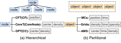
Figure 1: Six Types of Summarizing Data Structure in Benne.

3.1 Summarizing Data Structure

In Benne, the summarizing data structure plays a critical role in providing a compact representation of the data points within the stream. This abstraction helps to enhance computational efficiency while maintaining a low memory footprint. Depending on the clustering needs, Benne offers two categories of summarizing data structures: the hierarchical category and the partitional category.

3.1.1 Hierarchical Summarizing Data Structure

Hierarchical data structures are primarily used in Benne when the data streams display inherent hierarchies or when the data can be logically grouped into a tree structure. As shown in Figure 1(a), three types of hierarchical data structures are supported in Benne: Clustering Feature Tree (CFT), Coreset Tree (CoreT), and Dependency Tree (DPT).

Clustering Feature Tree (CFT). CFT [14] represents a classic yet efficient choice for hierarchical data representation in Benne. Its structure supports a broad range of basic operations required in stream clustering, such as distance calculation and cluster updating, thus providing a solid foundation for further complex manipulations.

Coreset Tree (CoreT). When the data stream is characterized by high volume and density variations, Benne employs CoreT [20] to extract a core subset for processing. Despite the necessity of full tree rebuilding during clustering, which could affect efficiency, the application of CoreT in Benne helps in obtaining high-quality clusters from dense data streams.

Dependency Tree (DPT). DPT [2] is Benne’s choice for handling cluster evolution effectively. The tree structure of DPT, specifically designed to adapt to evolving activities in the stream, ensures that Benne delivers high clustering accuracy even in dynamic environments.

3.1.2 Partitional Summarizing Data Structure

Partitional data structures, as shown in Figure 1(b), are beneficial when the data streams are best represented by flat, non-overlapping clusters. In Benne, these structures are used to effectively handle and categorize incoming data points into appropriate clusters. The algorithm supports three types of partitional data structures: Micro Clusters (MCs), Grids (Grids), and Augmented Meyerson Sketch (AMS).

Micro Clusters (MCs). MCs [16] serve as a means to reduce the computational load by representing a group of closely related data points as a single entity. With the additional elements for summarizing timestamps for clusters’ updates, MCs enable Benne to accurately track real-time clustering activities, especially under cluster evolution.

Grids (Grids). Benne uses Grids [15] when efficiency is paramount. The structure eliminates the need for frequent distance calculations between new data and the grid, boosting performance. Additionally, the periodic removal of sparse grids optimizes resource usage, while its fixed position may limit accuracy in cases of frequent evolving activities.

Augmented Meyerson Sketch (AMS). The AMS [19] is utilized for summarizing clustering information with a limited number of data points. Though it can be cost-intensive due to the need for sketch reconstruction to adapt to evolving data streams, it is applicable in scenarios where the exact number of clusters is known a priori. This flexibility helps Benne to accommodate diverse clustering needs.

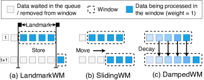
Figure 2: Three Types of Window Model.

3.2 Window Model

In Benne, the window model determines the scope of the data stream that is under consideration for clustering at any given time. The selected window model influences how Benne can adapt to evolving data distributions and concept drifts. As illustrated in Figure 2, the three primary types of window models supported in Benne are the Landmark Window Model (LandmarkWM), the Sliding Window Model (SlidingWM), and the Damped Window Model (DampedWM).

3.2.1 Landmark Window Model

In the LandmarkWM [39], the data stream is divided into fixed-size windows starting from a predefined landmark point. This model aids in detecting concept drifts and periodic patterns in the data by facilitating comparisons of clustering results across different windows. The primary challenge with the LandmarkWM lies in deciding the spacing between landmarks, which has an impact on clustering accuracy and efficiency.

3.2.2 Sliding Window Model

The SlidingWM [40, 19] focuses on a fixed-size window encompassing the most recent data points for clustering. As new data points are processed, the oldest ones are discarded, ensuring that the algorithm remains responsive to the latest trends in the data. This model may, however, compromise clustering accuracy, particularly when the window size is small.

3.2.3 Damped Window Model

The DampedWM [41, 15] assigns exponentially decaying weights to data points based on their age, giving precedence to recent data points while still considering older ones. This approach enables smoother adaptation to evolving data distributions. The DampedWM model is susceptible to certain stream characteristics, such as outlier effects, due to its predefined decay function parameters.

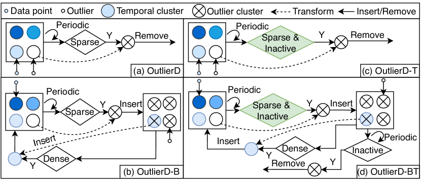
Figure 3: Four Types of Outlier Detection Mechanisms.

3.3 Outlier Detection Mechanism

Outlier detection mechanisms are optional design aspects in Benne that contribute to ensuring the quality of clustering results by identifying data points that deviate significantly from the overall data distribution. The two independent enhancements for this mechanism are the use of a buffer and a timer. We provide five variations, including not using any outlier detection mechanism (NoOutlierD). The other four variations are illustrated in Figure 3.

3.3.1 Basic Outlier Detection

As depicted in Figure 3(a), the Basic Outlier Detection (OutlierD) periodically identifies and removes low-density temporal clusters, improving clustering accuracy without significantly impacting efficiency [16, 15]. Outlier detection methods can be further categorized into distance-based, density-based, and grid-based approaches, each suited to particular data stream characteristics.

3.3.2 Outlier Detection with Buffer

The Buffer variant (OutlierD-B) retains potential outliers in a buffer for possible future clustering, as shown in Figure 3(b) [17, 2]. This approach improves the overall clustering performance by keeping the temporal clusters representative of the underlying data distribution and preventing the immediate incorporation of potential outliers.

3.3.3 Outlier Detection with Timer

The Timer variant (OutlierD-T) uses a timer mechanism, as illustrated in Figure 3(c), to evaluate the activity of temporal clusters before transforming them into outlier clusters. This method enhances the robustness of the outlier detection process and the overall accuracy of the clustering results. The trade-off is an increase in algorithmic complexity and the risk of preserving noisy clusters.

3.3.4 Outlier Detection with Buffer and Timer

As depicted in Figure 3(d), the combined Buffer and Timer variant (OutlierD-BT) retains outlier clusters in a buffer and uses a timer to evaluate their activity before transforming them into outlier clusters. Although this method improves the clustering accuracy, it increases the time required for buffer maintenance.

3.4 Refinement Strategy

The refinement strategy, an optional design aspect, helps to maintain the adaptability of DSC algorithms to evolving data distributions and concept drifts by updating the clustering model with new data points. Depending on computational efficiency, clustering accuracy, and adaptability to data distribution changes, there are three strategies available: NoRefine, One-shotRefine, and IncrementalRefine.

3.4.1 No Refinement

The NoRefine strategy, as depicted in Figure 4 (a), outputs the temporal clusters $C$ as the final results without further refinement. This strategy saves computational resources but may lower the clustering accuracy when handling evolving data distributions or concept drifts.

3.4.2 One-shot Refinement

The One-shotRefine strategy (Figure 4 (b)) performs model refinement less frequently to balance computational efficiency and clustering accuracy. This strategy is effective when computational resources are limited or the data stream changes gradually, allowing infrequent model updates.

3.4.3 Incremental Refinement

The IncrementalRefine strategy (Figure 4 (c)) updates the clustering model continuously as new data points arrive. This keeps the model current and adaptable but may increase computational overhead. The trade-off is improved clustering accuracy at the cost of computational complexity.

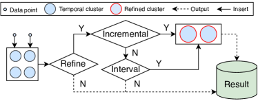
Figure 4: Refinement Strategies.

4 Design and Adaptability of Benne

This section elucidates the comprehensive algorithmic design of Benne. The algorithm is engineered for flexible adaptability, allowing it to self-adjust its design components in response to dynamically detected workload characteristics of the data stream and user-defined optimization objectives. This adaptability enables Benne to capitalize on the strengths of various design choices, thereby ensuring enhanced and stable clustering performance tailored to specific optimization goals.

4.1 General Workflow

Benne operates according to a bifurcated execution strategy, comprising an online phase and an offline phase. The algorithm’s adaptability is rooted in the flexible configuration of its core components: the summarizing data structure ($struc.$), window model ($win.$), outlier detection mechanism ($out.$), and refinement strategy ($ref.$). Guided by real-time stream characteristics, which are detected from a sample queue ($queue$), as well as predefined threshold values ($thresholds$) and a performance objective ($o$), Benne dynamically tailors its components to meet the specialized requirements of diverse applications and data streams. Algorithm 1 outlines the high-level execution flow of Benne. In the online phase, the algorithm sequentially processes incoming data points, adhering to the following steps:

Data: $p$ // Input point

1

Data: $c$ // Temporal Clusters

2

Data: $struc.$ // Type of summarizing data structure

3

Data: $win.$ // Type of window model

4

Data: $out.$ // Type of outlier detection mechanism

5

Data: $ref.$ // Type of refinement strategy

6

Data: $queue$ // Batch of stream for detection

7

Data: $thresholds$ // Identifying characteristics’ changes

8

Data: $o$ // User’s primary performance objective

9

// Online Phase

10 Initializing parameters and design choices ;

11 while !stop processing of input streams do

12       if $queue$ is full then

13             $struc\_{old}.$ = $struc.$ ;

14             $characteristics$ = Regular-detection Fun.(…) ;

15             $struc.$, $win.$, $out.$, $ref.$ = Auto-selection Fun.(…) ;

16             Flexible-migration Fun.(…);

17             Empty $queue$ ;

18            

19      else

20             $queue$.push($p$) ;

21            

22      Window Fun. (…);

23       if $out.$ != NoOutlierD then

24             $b$ $\leftarrow$ Outlier Fun. (…);

25             if $b$ = false then

                   Insert Fun. (…)// Insert $p$ to $s$ and update $s$

26                  

27            

28      else

             Insert Fun. (…)// Insert $p$ to $s$ and update $s$

29            

30      if $ref.$ = IncrementalRefine then

31             Refine Fun. ($ref.$);

32      

// Offline Phase

33 if $ref.$ = One-shotRefine then

34       Refine Fun. ($ref.$);

Algorithm 1 Execution flow of Benne.

(1) Automatic Design Choices Adaptation: Given the dynamic characteristics of data streams, Benne is designed to adapt its configuration to optimize performance continually. The algorithm accumulates incoming data points in a queue (denoted as $queue$ in Line 3 of Algorithm 1). It then performs real-time analysis of the stream’s characteristics using the Regular-detection Fun. (executed at Line 5). Based on this analysis, Benne dynamically selects the most suitable components for the current data stream using the Auto-selection Fun. (executed at Line 6). Detailed discussions of these functions are available in Sections 4.2 and 4.3. If a change in the summarizing data structure is warranted, Benne transfers the temporal clusters from the old structure ($struc.\_old$) to the new one ($struc.$) using the Flexible-migration Fun. (executed at Line 7), as elaborated in Section 4.4.

(2) Window Function: The Window Fun. (executed at Line 11 in Algorithm 1) manages the data points in the summarizing data structure ($s$), in accordance with the selected window model ($win.$). This function ensures that the algorithm’s focus remains on the most recent and relevant data points, thereby allowing it to adapt to changes in the data distribution effectively.

(3) Outlier Detection: When the outlier detection mechanism ($out.$) is activated, the algorithm invokes the Outlier Fun. to assess if the current input point ($p$) qualifies as an outlier. This function is executed between Lines 12-15 in Algorithm 1. If the point is determined not to be an outlier, it is subsequently inserted into the summarizing data structure ($s$) and the structure is updated accordingly (executed at Line 15). Conversely, if the outlier detection mechanism is deactivated, the input point is directly inserted into the summarizing data structure, as indicated at Line 17 in Algorithm 1.

(4) Incremental Refinement: Should the refinement strategy ($ref.$) be configured to IncrementalRefine, the algorithm invokes the Refine Fun. each time new data points are processed. This is executed between Lines 18-19 in Algorithm 1. This strategy ensures that the clustering model is continuously updated and remains responsive to dynamic changes in the data distribution. However, this approach may necessitate more frequent updates, thereby potentially increasing computational overhead.

(5) One-shot Refinement: Upon completion of the input data stream processing, the algorithm transitions to the offline phase. If the refinement strategy ($ref.$) is configured as One-shotRefine, the Refine Fun. is executed in a single pass at the conclusion of the stream processing, as indicated between Lines 20-21 in Algorithm 1. This strategy minimizes computational overhead by limiting the frequency of refinement operations. However, it may compromise the adaptability of the clustering model if it fails to capture timely changes in the data distribution.

4.2 Regular Stream Characteristics Detection

As elaborated in Section 2.2, various stream characteristics such as data dimensionality, cluster evolution, and the number of outliers are subject to change in evolving data streams. To make informed decisions about the most appropriate design choices for real-time clustering, Benne must first ascertain the current characteristics of the data stream. Algorithm 2 delineates the procedure Benne employs to automatically detect key attributes like dimensionality, cluster evolution, and the number of outliers in the current data stream.

/* $queue$: a queue of new input stream data stored for detecting stream characteristic changes, $centers$: previous clustering centers of the stream data, $thresholds$: threshold values for identifying the characteristic */

1 Function Regular-detection Fun.($queue,centers,threshold$):

       /* Initialize stream characteristics */

2       $characteristics$ = null;

3       $high\_dim\_data$ = $var$ = $num\_of\_outliers$= 0;

4       $new\_center$ = mean($queue$);

5       for $s\in queue$ do

6             if $s.dim>T_{d}$ then

7                   $high\_dim\_data$ += 1 ;

8                  

9            $var$ = UpdateVariance($var,s,new\_centers$);

10             if $min(dist(s,centers))>thresholds.dist$ then

11                   $num\_of\_outliers$ += 1 ;

12                  

13            

14      if $high\_dim\_data>num(samples)/2$ then

15             $characteristics.high\_dimension=true$ ;

16            

17      else

18             $characteristics.high\_dimension=false$ ;

19            

20      if $var>thresholds.variance$ then

21             $characteristics.frequent\_evolution=true$ ;

22            

23      else

24             $characteristics.frequent\_evolution=false$ ;

25            

26      if $num\_of\_outliers>num(samples)/2$ then

27             $characteristics.many\_outliers=true$ ;

28            

29      else

30             $characteristics.many\_outliers=false$ ;

31            

32      Return $characteristics$;

Algorithm 2 Regular-detection Fun. of Benne

Specifically, the algorithm initializes various counters and variables to store stream characteristics at Lines 3-5 of Algorithm 2. For each new data point in the $queue$ (Line 6), Benne evaluates its dimensionality. If the dimension exceeds the threshold $T_{d}$, the counter $high\_dim\_data$ is incremented (Line 7). The variance of the data stream is updated at Line 8. The algorithm also checks whether each data point is an outlier based on its distance to the current clustering centers (Line 9-10).

After processing all the data points in the $queue$, Benne sets the $characteristics.high\_dimension$ attribute to “true” or “false” based on the value of $high\_dim\_data$ (Lines 11-14). Similarly, the $characteristics.frequent\_evolution$ attribute is determined based on the calculated variance (Lines 15-19), and the $characteristics.many\_outliers$ attribute is set based on the number of outliers detected (Lines 20-23).

/* $objective$: User’s primary performance objective (Accuracy, Efficiency, or Balance); $data$: Input data stream; $characteristics$: Stream characteristics detected by regular-detect Fun. */

1 Function Auto-Selection Fun.($objective$, $data$, $characteristics$):

       /* Initialize four modular design components */

2       $struc.$= $win.$ = $out.$= $ref.$ = null;

3       if $objective$ = Accuracy then

             /* Select modules with high accuracy based on input data stream characteristics */

4             if $characteristics.frequent\_evolution=true$ then

5                   $struc.$ = MCs ;

6                  

7            else

8                   $struc.$ = CFT ;

9                  

10            if $characteristics.many\_outliers=true$ then

11                   $win.$ = LandmarkWM ;

12                   $out.$ = OutlierD-BT ;

13                  

14            else

15                   $win.$ = DampedWM ;

16                   if $characteristics.high\_dimension=true$ then

17                         $out.$ = OutlierD-B ;

18                        

19                  else

20                         $out.$ = OutlierD-BT ;

21                        

22                  

23            $ref.$ = IncrementalRefine ;

24            

25      else

             /* Choose a structure with high efficiency based on input data stream characteristics */

26             if $characteristics.frequent\_evolution=true$ then

27                   $struc.$ = DPT ;

28                   $win.$ = LandmarkWM ;

29                  

30            else

31                   $struc.$ = Grids ;

32                   $win.$ = SlidingWM ;

33                  

34            $out.$ = NoOutlierD ;

35             $ref.$ = NoRefine ;

36            

37      

38      Return $struc.$, $win.$, $out.$, $ref.$;

Algorithm 3 Auto-selection Fun. of Benne

4.3 Automatic Design Choice Selection

Upon receiving the stream characteristics from the Regular-detection Function, Benne proceeds to select the most appropriate design choices based on these characteristics and the user-defined optimization objective. The detailed selection process is delineated in Algorithm 3.

If the optimization objective is set to Accuracy (Line 3), Benne selects the summarizing data structure based on the frequency of cluster evolution. Specifically, MCs is chosen if frequent cluster evolution is detected (Line 6), otherwise CFT is selected (Line 8). For the window model and outlier detection mechanisms, Benne selects LandmarkWM and OutlierD-BT if many outliers are present (Lines 10-11). If outliers are scarce, DampedWM is chosen as the window model, and the choice between OutlierD-B and OutlierD-BT for outlier detection is influenced by the data’s dimensionality (Lines 13-16). The refinement strategy is set to IncrementalRefine (Line 18).

If the optimization objective is set to Efficiency (Line 20), Benne selects either DPT or Grids as the summarizing data structure based on the frequency of cluster evolution (Lines 22-25). The window model is also selected accordingly, with LandmarkWM chosen for frequent cluster evolution and SlidingWM otherwise (Lines 24-25). The outlier detection mechanism is set to NoOutlierD (Line 26), and the refinement strategy is set to NoRefine (Line 27).

/* $objective$: User’s primary performance objective (Accuracy or Efficiency); $struc.$: New selected summarizing data structure; $struc\_{old}.$: Previous selected summarizing data structure; $out.$: Previous selected outlier detection mechanism */

1 Function Flexible-migration Fun.($objective$, $struc.$, $struc\_{old}.$):

2       if $struc.$ != $struc\_{old}.$ then

3             Extract the clustering centers $c$ from $struc.$;

4             if $objective$ = Accuracy then

                   /* Transfer the old clustering results to the new summarizing data structures for the accuracy or balance objective */

5                   if $out.$ = OutlierD-B or OutlierD-BT then

6                         Extract the outliers $o$ from $out.$;

7                        

8                  Initialize the new summarizing data structure $struc.$ with $c$ and $o$;

9                  

10            else

                   /* Sink the old clustering results for the efficiency objective */

11                   Sink $c$ into the output;

12                   Create a blank object for initializing $struc.$;

13                  

14            

15      

Algorithm 4 Flexible-migration Fun. of Benne.

4.4 Flexible Algorithm Migration

Due to the significant structural differences among various summarizing data structures, as elaborated in Section 3.1, it is not feasible to directly transfer clustering information from the old summarizing data structure to the new one. To address this, Benne employs a migration function, delineated in Algorithm 4.

Specifically, if the newly selected summarizing data structure ($struc.$) differs from the previously selected one ($struc\_{old}.$) (Line 2), the algorithm proceeds as follows:

• Accuracy Objective (Lines 4-7): If the optimization objective is Accuracy, Benne extracts the clustering centers ($c$) from the old summarizing data structure (Line 3). Additionally, if the old outlier detection mechanism ($out.$) is either OutlierD-B or OutlierD-BT, outliers ($o$) are also extracted (Line 6). These centers and outliers are then used to initialize the new summarizing data structure ($struc.$) (Line 7).

• Efficiency Objective (Lines 8-10): If the optimization objective is Efficiency, Benne extracts the clustering centers ($c$) from the old summarizing data structure and sinks them into the output to avoid computational overhead (Line 9). A new, empty object is created to initialize the new summarizing data structure ($struc.$) (Line 10).

This approach ensures that Benne can smoothly transition between different summarizing data structures while optimizing for the user-defined objective.

4.5 Modular Composition of Clustering Functions

The clustering process, as delineated from Lines 11 to 21 in Algorithm 1, comprises four primary functions, each responsible for a specific aspect of the algorithm’s operation.

4.5.1 Window Function

The Window Fun. (Algorithm 5) employs distinct computational logic contingent upon the selected window model. The function maintains a counter $c$ to monitor the number of processed data points and executes specific actions based on the chosen window model.

Landmark Window (Lines 4-8): When the landmark window model is activated, the function assesses whether the counter $c$ has exceeded the current landmark $m$. If affirmative, the clustering results in the summarizing data structure $s$ are sunk, either stored or output, and all existing clustering information is purged. The function then updates the current landmark to $m_{\text{next}}$ for the subsequent window. This model is particularly beneficial in contexts where the data distribution experiences significant fluctuations, requiring the algorithm to adapt by periodically resetting its clustering information.

Damped Window (Lines 9-10): In the damped window model, the function adjusts the weights of data points and clusters in the summarizing data structure $s$ using decay parameters $dc=(\alpha,\lambda)$. This model is tailored for situations where older data points should exert less influence on the clustering results. By implementing a decay function, the algorithm can incrementally discard outdated information and adapt to the current data distribution.

Sliding Window (Lines 11-13): If the sliding window model is selected, the function verifies whether the counter $c$ has surpassed the sliding window size $ws$. If so, the earliest data point in the window is removed from the summarizing data structure $s$. This model maintains a fixed-size window of the most recent data points, ensuring that the algorithm concentrates on the current data distribution while disregarding older, potentially irrelevant, data points.

/* $c$: counter (initialized with 0), $m$: landmark, $ws$: sliding window size, $dc=(\alpha,\lambda)$: decay parameters */

1 Function Window Fun.($s$, $m$, $ws$, $dc$):

2       $c$++;

3       if $win.$ = LandmarkWM then

4             if $c>$ $m$ then

5                   Sink the clustering results from $s$;

6                   Clear all of the clustering information;

                   $m$ $\leftarrow$ $m_{next}$; /* update current landmark */

7                  

8            

9      else

10            if $win.$ = DampedWM then

11                   Update weight with $dc$;

12                  

13            else // $win.$ = SlidingWM

14                   if $c>$ $ws$ then

15                         Remove the earliest point from window;

16                        

17                  

18            

19      

Algorithm 5 Window Fun. of Benne.

/* $Buffer$: outlier buffers, $t$: timer threshold, $d$: density threshold */

1 Function Outlier Fun.($p$, $s$, $Buffer$, $t$, $d$):

2       if $out.$ = (OutlierD-B Or OutlierD-BT) then

             /* use buffer optimization */

3             if ($p$ Is Outlier) = true then

4                   Select cluster $cl$ closest to $p$ from $Buffer$;

5                   Insert $p$ to $cl$ and update $cl$;

6                   bool $dense\leftarrow$ Check ($cl$);

                   /* check if $cl$ is dense enough */

7                   if $dense$ = true then

8                         Move $cl$ from $Buffer$ to $s$;

9                        

10                  

11            

12      if REGULAR CHECK TRIGGERED then

             $cls\leftarrow$ Extract($s$);/* extract all clusters from $s$ */

13             for $cl\in cls$ do

14                   bool $active$ = false;

15                   bool $dense\leftarrow$ Check ($cl,d$);

                   /* check if $cl$ is dense enough */

16                   if $out.$ = (OutlierD-T Or OutlierD-BT) then

                         /* use timer optimization */

17                         bool $active\leftarrow$ Check($cl.timer,t$);

                         /* check if $cl$ is active enough */

18                        

19                  if $dense$ = false and $active$ = false then

20                         if BUFFER ENABLED then

21                               Insert $cl$ to $Buffer$;

22                              

23                        Remove $cl$ from $s$;

24                        

25                  

26            if OutlierD-BT then

27                   for $cl\in Buffer$ do

28                         bool $active\leftarrow$ Check($cl.timer,t$);

29                         if $active$ = false then

30                               Remove $cl$ from $Buffer$;

31                              

32                        

33                  

34            

35      Return ($p$ Is Outlier);

36      

Algorithm 6 Outlier Fun. of Benne.

4.5.2 Outlier Function

When outlier detection is activated, the Outlier Fun. (Algorithm 6) comes into play. This function is pivotal in the outlier detection mechanism of the Benne algorithm, managing outliers through various strategies depending on the selected outlier detection type ($out.$). Below is an in-depth discussion of the steps involved in Outlier Fun.:

Buffer Optimization (Lines 2-8): When either buffer or buffertimer is the chosen outlier detection mechanism, the function evaluates whether the input point $p$ is an outlier. If $p$ qualifies as an outlier, it is inserted into the outlier buffer ($Buffer$) and allocated to the nearest cluster ($cl$). Subsequently, the cluster within the buffer is updated. The function then ascertains if the cluster has sufficient density, exceeding the predefined density threshold $d$. If the cluster meets the density criteria, it is transferred from the outlier buffer to the summarizing data structure $s$.

Regular Check (Lines 9-24): This check is initiated at predetermined intervals to scrutinize the clusters in both the summarizing data structure and the outlier buffer. For each cluster in the summarizing data structure, the function evaluates its density against the threshold $d$ and, if a timer-based mechanism (timer or buffertimer) is in use, its activity against the timer threshold $t$. If a cluster is neither sufficiently dense nor active, it is either relocated to the outlier buffer (if enabled) or excised from the summarizing data structure.

Buffer Timer Check (Lines 20-24): In cases where buffertimer is the selected outlier detection mechanism, the function assesses the activity level of each cluster in the outlier buffer using the timer threshold $t$. Clusters deemed inactive are purged from the buffer.

Outlier Determination (Line 25): The function concludes by returning a boolean value indicating whether the input point $p$ is an outlier, based on the outcomes of the preceding steps.

4.5.3 Insert Function

The Insert Fun. (Algorithm 7) is invoked to insert the input point $p$ into the designated summarizing data structure $struc.$. This function is designed to be versatile, accommodating both hierarchical and partitional types of summarizing data structures. This adaptability ensures that Benne can efficiently manage a range of summarizing data structures, thereby meeting diverse application needs.

When the selected data structure is of the hierarchical category, the function incorporates the input point $p$ into the appropriate cluster within the hierarchical structure and subsequently updates the hierarchy (Lines 2-3). Conversely, if the data structure is partitional, the function initially identifies the closest cluster to the input point $p$, inserts $p$ into this cluster, and then updates the partitional structure accordingly (Lines 4-5).

/* $p$: input, $struc.$: summarizing data structure */

1 Function Insert Fun.($p$, $struc.$):

2       if $struc.$ belongs to hierarchical category then

             /* Insert $p$ into the hierarchical data structure and update it */

3             Insert $p$ into the appropriate cluster in the hierarchy; Update the hierarchy based on the insertion;

4      else

             /* Insert $p$ into the partitional data structure and update it */

5             Find the closest cluster for $p$; Insert $p$ into the closest cluster; Update the partitional data structure based on the insertion;

6      

Algorithm 7 Insert Fun. of Benne.

4.5.4 Refine Function

The Refine Fun. (Algorithm 8) is designed to refine the clustering results based on the chosen refinement strategy, denoted as $ref.$. The algorithm offers two refinement strategies: IncrementalRefine and One-shotRefine, each catering to specific application requirements and data stream dynamics.

In the case of IncrementalRefine, the function invokes the ExtractModel and UpdateModel steps (see Algorithm 8). It first extracts the current clustering model from the summarizing data structure $s$ and then applies a suitable batch clustering algorithm to update it. Following this, the UpdateStructure and CleanStructure steps are executed to update $s$ with the new model and to remove any outdated or redundant data points or clusters, respectively. This ensures that the model is continually updated to adapt to evolving data distributions.

On the other hand, when One-shotRefine is selected, the function performs the ExtractAll step to retrieve all clusters and data points from $s$. A batch clustering algorithm is then applied during the RefineModel step to improve the clustering results. Finally, the UpdateStructure step updates $s$ with the refined clustering model, offering a more accurate snapshot of the current data distribution.

/* $ref.$: Refinement strategy, $s$: Summarizing data structure */

1 Function Refine Fun.($ref.$, $s$):

2       if $ref.$ = IncrementalRefine then

             ExtractModel($s$); /* Get current model */

             UpdateModel(); /* Batch clustering */

             UpdateStructure($s$); /* Update $s$ */

             CleanStructure($s$); /* Remove outdated data */

3            

4      else

             ExtractAll($s$); /* Get all clusters and points */

             RefineModel(); /* Batch clustering */

             UpdateStructure($s$); /* Update $s$ */

5            

6      

Algorithm 8 Refine Fun. of Benne.

5 Experimental Analysis

In this section, we present the evaluation results. All experiments are carried out on an Intel Xeon processor. Table II summarizes the detailed specification of the hardware and software used in our experiments.

TABLE II: Specification of our evaluation platform

Component	Description
Processor	Intel(R) Xeon(R) Gold 6338 CPU @ 2.00GHz
L3 Cache Size	48MiB
Memory	256GB DDR4 RAM
OS	Ubuntu 20.04.4 LTS
Kernel	Linux 5.4.0-122-generic
Compiler	GCC 11.3.0 with -O3

5.1 Implementation Details

Benne is architected as a three-threaded pipeline to process data streams, thereby approximating a realistic computational environment. Inter-thread communication is facilitated through a shared-memory queue, mitigating the latency associated with network transmissions.

The first thread, termed as the Data Producer Thread, is responsible for loading benchmark workloads into memory. It then sequentially enqueues each data point into a shared queue. To simulate a high-throughput scenario, the input arrival rate is configured to be immediate, thereby eliminating idle time for the algorithm.

The second thread, known as the Data Consumer Thread, executes a DSC algorithm to process the incoming data stream. It dequeues input tuples from the shared queue for processing and subsequently generates temporal clustering results. These results are then forwarded to the next thread in the pipeline. Notably, all efficiency metrics are captured in this thread to ensure a consistent basis for comparing various DSC algorithms.

Finally, the Result Collector Thread serves as the repository for the temporal clustering results generated by the Data Consumer Thread. Accuracy metrics are computed in this thread to minimize any interference with efficiency measurements. The quality of clustering is evaluated using purity [25], and the capability of the design aspects to handle cluster evolution is assessed using CMM [26].

TABLE III: A summary of representative DSC algorithms and their design decisions. The year attribute for each algorithm is when it was first published.

Algorithm	Year	Summarizing Data Structure		Window Model	Outlier Detection	Offline Refinement
		Name	Catalog
BIRCH [14]	1996	CFT	Hierarchical	LandmarkWM	OutlierD	IncrementalRefine
CluStream [16]	2003	MCs	Partitional	LandmarkWM	OutlierD-T	IncrementalRefine
DenStream [41]	2006	MCs	Partitional	DampedWM	OutlierD-BT	One-shotRefine
DStream [15]	2007	Grids	Partitional	DampedWM	OutlierD-T	One-shotRefine
StreamKM++ [20]	2012	CoreT	Hierarchical	LandmarkWM	NoOutlierD	One-shotRefine
DBStream [18]	2016	MCs	Partitional	DampedWM	OutlierD-T	One-shotRefine
EDMStream [2]	2017	DPT	Hierarchical	DampedWM	OutlierD-BT	IncrementalRefine
SL-KMeans [19]	2020	AMS	Partitional	SlidingWM	NoOutlierD	IncrementalRefine

5.2 Algorithm Selection

In our comparative analysis, Benne is benchmarked against eight established DSC algorithms, summarized in Table III. The selection of these algorithms is guided by two primary criteria: 1) they collectively represent a broad spectrum of design decisions across all four design aspects, as detailed in Table III; 2) they span a historical range in the field, from foundational algorithms like BIRCH [14] to contemporary contributions such as SL-KMeans [19].

The BIRCH algorithm [14], a seminal work in this domain, introduced the concept of Clustering Feature (CF) for data summarization. This idea was later extended to Micro Cluster (MC) in CluStream [16], which pioneered the online-offline strategy for efficient stream clustering. DenStream [17] builds upon CF and incorporates outlier detection to mitigate the influence of noise.

DStream [15] employs a unique approach by partitioning the feature space into density cells and mapping data objects into these cells. In contrast, StreamKM++ [20] utilizes a two-step “merge and split” mechanism centered around a Coreset Tree data structure. DBStream [18] addresses the fragmentation of dense areas in micro-cluster-based algorithms, while EDMStream [2] employs a damped window model to allow cluster density to decay over time. Lastly, SL-KMeans [19] introduces algorithms for $k$-clustering on sliding windows, demonstrating superior performance over analytical bounds.

TABLE IV: Characteristics differences of selected workloads. Note that the outliers column refers to whether there are outliers in the final clustering results.

Workload	Length	Dim.	Cluster Num.	Outliers	Evolving Freq.
FCT [42]	581012	54	7	False	Low
KDD99 [1]	4898431	41	23	True	Low
Insects [43]	905145	33	24	False	Low
Sensor [44]	2219803	5	55	False	High
EDS [17]	245270	2	363	False	Varying
ODS [17]	100000	2	90	Varying	High
ES [17]	345270	2	453	Varying	Varying
Dim [45]	500000	20$\sim$100	50	Low	Low

5.3 Dataset Selection

Table IV provides a summary of the datasets selected for evaluation. Our dataset selection is governed by two primary criteria. First, we aim for a fair and comprehensive evaluation by including the three most frequently used datasets across the algorithms summarized in Table III. Specifically, FCT (Forest CoverType) is employed by algorithms such as SL-KMeans, StreamKM++, EDMStream, and DBStream. The KDD99 dataset is utilized by StreamKM++, DStream, EDMStream, DenStream, CluStream, and DBStream, while Sensor is specifically used by DBStream. In addition to these three classical datasets, we incorporate a more recent dataset, Insects, which was proposed in 2020 [43].

Second, although some previous studies have proposed synthetic datasets, these datasets are not publicly available. To address this limitation and to evaluate the algorithm under varying workload characteristics, as delineated in Table IV, we design three synthetic datasets: EDS, ODS, and Dim. The EDS dataset contains varying frequencies of the occurrence of cluster evolution, ODS features a time-varying number of outliers at different stages, and Dim comprises data points with extremely high dimensions.

A more detailed account of each dataset is as follows:

• FCT (Forest CoverType) [42] consists of tree observations from four areas of the Roosevelt National Forest in Colorado. It is a high-dimensional dataset with 54 attributes, and each data point has a cluster label indicating its tree type. The dataset contains no outliers.

• KDD99 [1] is a large dataset of network intrusion detection stream data collected by the MIT Lincoln Laboratory. It is also high-dimensional and contains a significant number of outliers, making it suitable for testing outlier detection capabilities.

• Insects [43] is the most recent dataset, generated by an optical sensor that measures insect flight characteristics. It is specifically designed for testing the clustering of evolving data streams.

• Sensor [44] contains environmental data such as temperature, humidity, light, and voltage, collected from sensors deployed in the Intel Berkeley Research Lab. It is a low-dimensional dataset with only five attributes but has a high frequency of cluster evolution.

• EDS is a synthetic dataset used in previous works [17] to study cluster evolution. It is divided into five stages according to evolving frequency, allowing for a comparative analysis of algorithmic performance across these stages.

• ODS is another synthetic dataset, distinct from EDS in that its second half is composed entirely of outliers, enabling an analysis of algorithmic performance under varying numbers of outliers.

• Dim is generated using the RandomTreeGenerator from the MOA framework [45]. It features data points with dimensions ranging from 20 to 100 and 50 classes, with other specific configurations set to default.

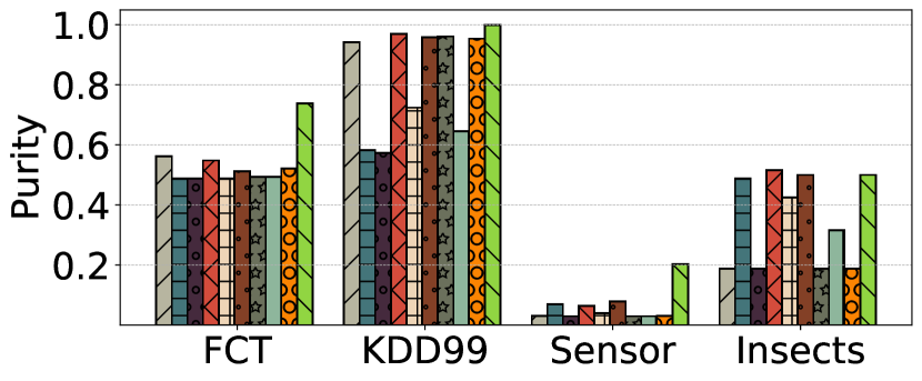
(a) Accuracy

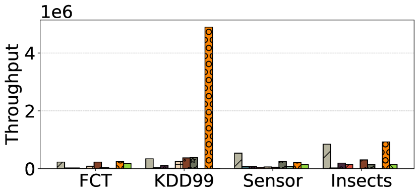
(b) Efficiency

Figure 5: Performance Comparison on Four Real-world Workloads.

5.4 General Evaluation of Clustering Behavior

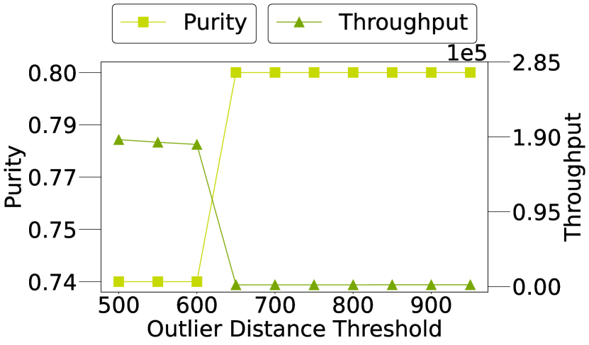
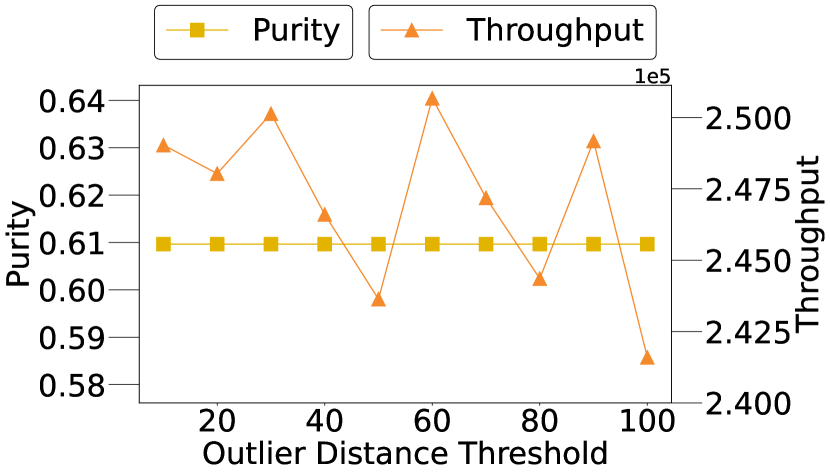
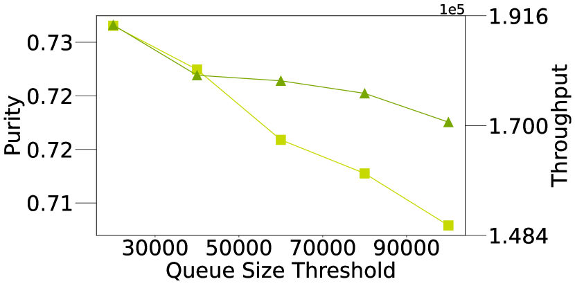
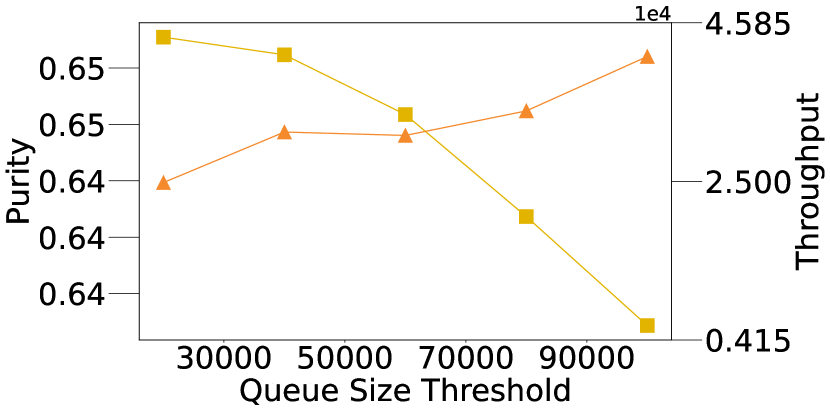
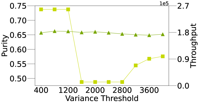
(a) Benne (Accuracy)

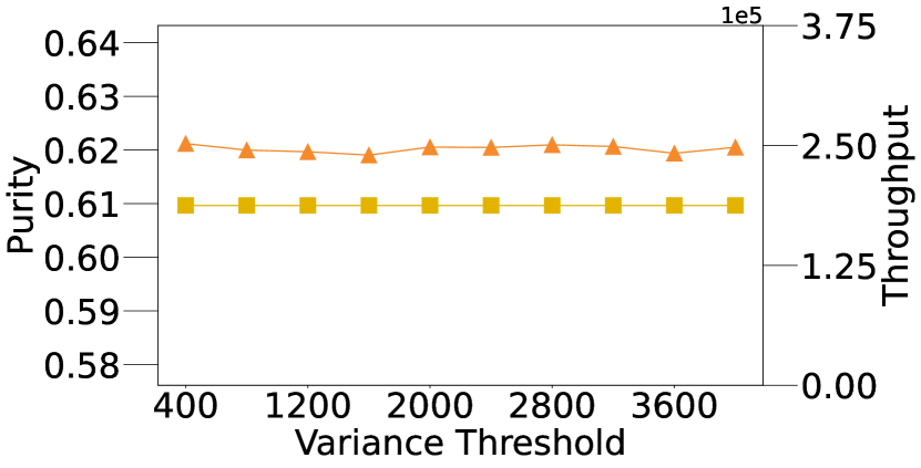
(b) Benne (Efficiency)

Figure 11: Parameter Analysis of Benne variants on FCT.

The versatility of Benne allows it to be configured into two primary variants: Benne (Accuracy) and Benne (Efficiency). These variants are tailored to different optimization objectives and are derived from distinct algorithmic design decisions. We initiate our evaluation by comparing the clustering behavior of these Benne variants with eight existing DSC algorithms. The evaluation is conducted on four real-world datasets—FCT, KDD99, Insects, and Sensor —as well as two evolving datasets—EDS and ODS. The outcomes are illustrated in Figure 5, Figure 6, and Figure 11, yielding two key insights.

First, Figure 5 reveals that Benne (Accuracy) attains state-of-the-art purity across all four real-world datasets. Conversely, Benne (Efficiency) exhibits purity levels comparable to existing algorithms but surpasses them in throughput. These observations confirm that by judiciously selecting and integrating different design elements, as elaborated in Section 4.5, both Benne variants can either optimize for accuracy or efficiency. However, achieving both optimal accuracy and efficiency simultaneously remains elusive, corroborating our initial analysis regarding the trade-off between these two metrics.

Second, Figures 6 and 11 demonstrate the robustness of both Benne variants in evolving scenarios. Specifically, Benne (Accuracy) and Benne (Efficiency) maintain their respective optimization targets even under frequent cluster or outlier evolution. This stability contrasts with the deteriorating performance observed in several existing DSC algorithms, such as DStream and SL-KMeans, which struggle to adapt to evolving conditions. We attribute this resilience to Benne’s dynamic composition capability, as discussed in Section 4. Unlike most existing algorithms, Benne continuously monitors stream characteristics to detect any changes, thereby enabling timely and accurate adaptations to the evolving data stream. This dynamic adaptability ensures superior clustering performance under varying conditions.

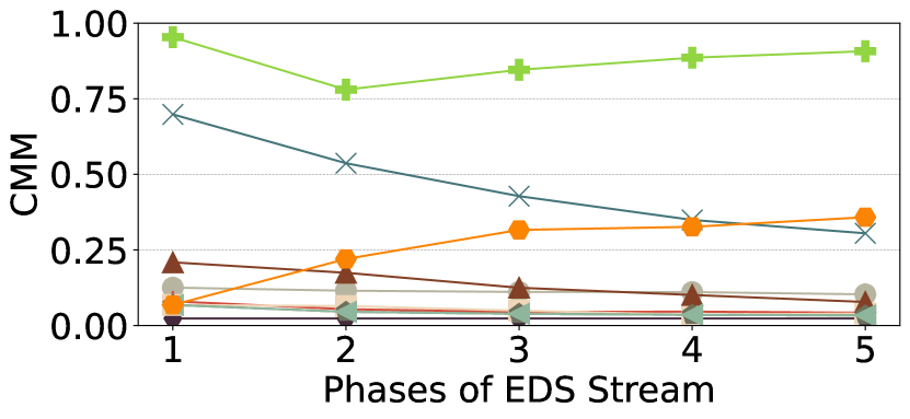
(a) Accuracy

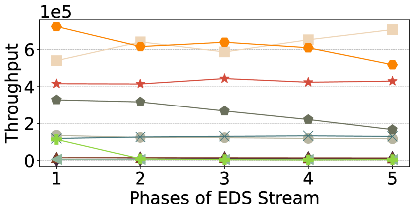
(b) Efficiency

Figure 6: Performance Comparison on EDS workload with varying cluster evolution frequency.

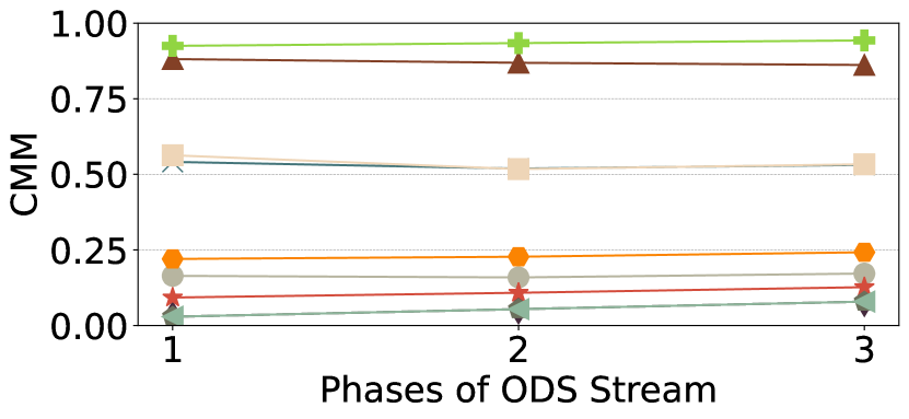
(a) Accuracy

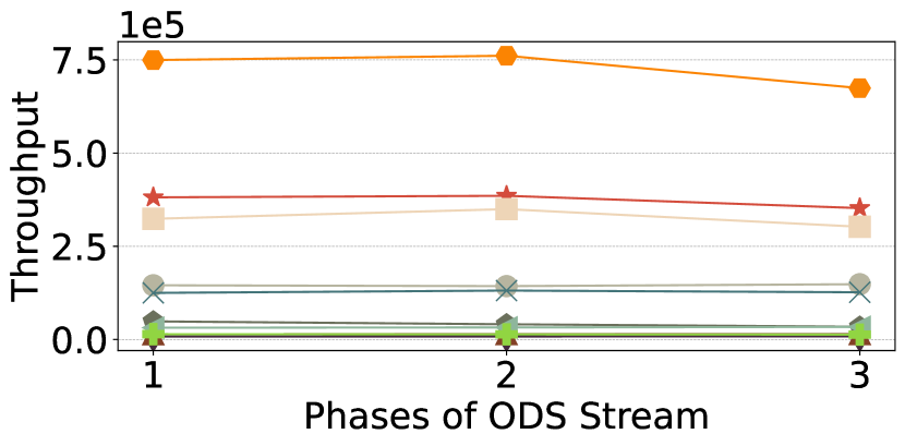
(b) Efficiency

Figure 7: Performance Comparison on ODS workload with varying outlier evolution frequency.

5.5 Analysis of Dynamic Composition Ability

We then conduct a detailed analysis to show the effectiveness of Benne’s critical ability for dynamic composition, including regular stream characteristics detection (Section 4.2), automatic choice selection (Section 4.3) and flexible algorithm migration (Section 4.4) respectively under the evolving workload characteristics.

Specifically, to measure the role of the regular stream characteristics detection module, we estimate the general location where the stream characteristics evolve in the workload and check whether the evolution has been detected timely and accurately based on the output of the regular detection function of Benne as discussed in Algorithm 2. To show the effectiveness of the last two modules, we add two other variants, one is Benne (Accuracy) without migration, and the other is Benne (Efficiency) without selection. By comparing the changes in both clustering purity and throughput of the total four variants of Benne, we are able to identify the real functionality of the last two modules of dynamic composition.

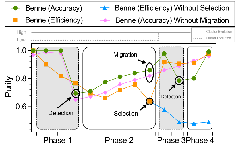
(a) Accuracy

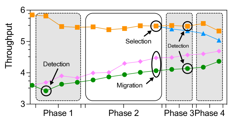
(b) Efficiency

Figure 8: Detailed performance analysis of Benne’s variants on KDD99.

5.5.1 Composition Effectiveness Study

We commence by evaluating the performance of the four Benne variants on the real-world KDD99 workload, characterized by a high frequency of outliers but low cluster evolution, as detailed in Table IV. Measurements are taken at intervals of 40,000 data points, capturing both clustering outcomes and workload characteristic evolutions, as illustrated in Figure 8. Notably, Benne (Accuracy) excels in purity, while Benne (Efficiency) demonstrates superior throughput, each aligning with their respective optimization objectives. Three key observations emerge from this analysis.

First, a synchronized examination of Benne’s clustering behavior and workload evolution (indicated by grey lines in the figure) reveals that while workload changes adversely affect clustering performance (evident in Phases 1 and 3), both Benne (Accuracy) and Benne (Efficiency) swiftly recover (Phases 2 and 4).

For Benne (Accuracy), the initial use of the DampedWM window model leads to a rapid decline in both purity and throughput during Phase 1 due to its inability to effectively manage increasing outlier frequencies. However, the algorithm’s regular stream characteristics detection module, as outlined in Algorithm 2, timely identifies this issue at the close of Phase 1, transitioning to the LandmarkWM window model to better cope with outlier evolution. The subsequent improvement in purity during Phase 2 attests to the efficacy of this module. A similar recovery is observed in Phase 4, where the algorithm switches from CFT to MCs to adapt to increasing cluster evolution in Phase 3.

For Benne (Efficiency), the algorithm opts to forgo outlier detection to minimize overhead, in line with its optimization target. Consequently, its performance deteriorates in Phases 1 and 2. However, upon entering Phase 3, characterized by high cluster evolution, the algorithm promptly detects this change and switches from Grids to DPT, resulting in improved purity and throughput in Phase 4, as depicted in Figure 8.

Second, apparently, both the purity and throughput drops significantly when canceling the usage of automatic design choice selection and switching, as shown by Benne (Efficiency) without selection. This indicates the limitation of the individual composition, as discussed in Section 3. On the contrary, applying the automatic design choice selection into the algorithm can make full use of the strengths of every design choices, leading to both better clustering accuracy and efficiency, as shown by Benne (Efficiency),

Third, the inclusion of migration in the algorithm improves accuracy at the expense of clustering speed. A comparative analysis of Benne (Accuracy) and Benne (Accuracy) without migration reveals that while the former consistently outperforms the latter in purity, it lags in throughput. A detailed assessment of the overhead incurred by the three dynamic composition modules will be presented in the subsequent section.

5.5.2 Analysis of Composition-Related Overhead

We proceed to examine the computational overhead associated with Benne’s two pivotal composition procedures: detection and migration. This is juxtaposed against the time expended on clustering, contingent on the selected composition. As illustrated in Figure 9, the time allocation for both detection and migration is relatively minimal for Benne (Accuracy) in comparison to the primary clustering task. This underscores the efficiency of these composition procedures.

In the case of Benne (Efficiency), the scenario is somewhat different. Given that this variant is optimized for speed, the clustering operation itself is more time-efficient. Consequently, the proportion of time spent on the detection procedure appears to be larger relative to Benne (Accuracy). However, it’s crucial to note that Benne (Efficiency) omits the migration procedure altogether, as elaborated in Section 4.4. This strategic omission further enhances its efficiency, aligning it closely with its optimization objectives.

This analysis confirms that the overheads associated with dynamic composition in Benne are well-contained, thereby not compromising the algorithm’s primary objectives of either accuracy or efficiency.

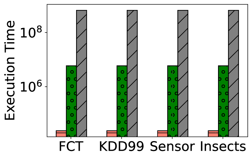
(a) Accuracy

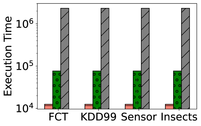
(b) Efficiency

Figure 9: Execution Time Break Down Analysis on Real-world Workloads.

5.6 Scalability Across Dimensions

We turn our attention to evaluating the scalability of Benne in the context of varying dimensions, utilizing the Dim workload for this purpose. This workload comprises datasets with dimensions ranging from 20 to 100, as detailed in Table IV. The outcomes of this evaluation are graphically represented in Figure 10.

Remarkably, Benne maintains a stable purity level of approximately 0.4 across datasets with diverse dimensions. While this purity level may not be high, its consistency is noteworthy, particularly when contending with the Curse of Dimensionality. Operations integral to clustering—such as updating the summarizing data structure and pinpointing the appropriate cluster for data insertion—are intrinsically reliant on distance calculations involving the original high-dimensional data. The efficacy of these distance metrics tends to wane as the dimensionality escalates, thereby exacerbating the challenge of distinguishing between data points in high-dimensional spaces.

Additionally, we discern a decrement in Benne’s efficiency concomitant with an increase in the dataset’s dimensionality. Our analysis ascertains that the computational complexity of several pivotal operations—including but not limited to the updating of the summarizing data structure and the selection of suitable clusters for data insertion—is directly influenced by the dimensionality of the workload. Consequently, a surge in dimensionality incurs a proportional rise in the computational time required for these operations, thereby attenuating the overall efficiency of the clustering process.

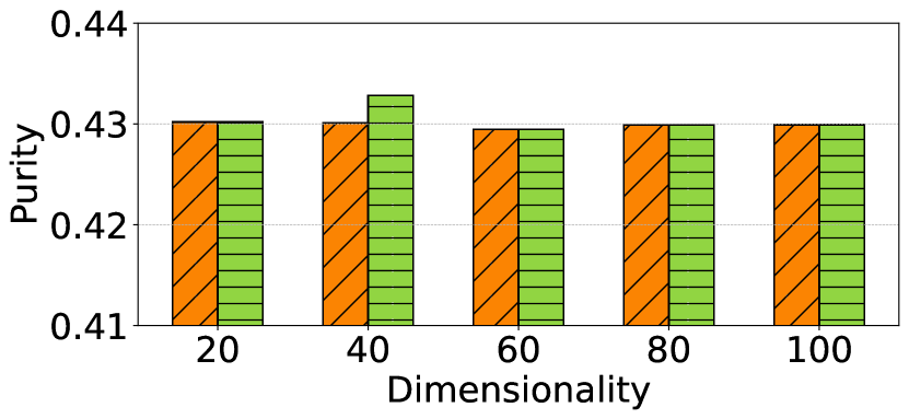
(a) Accuracy

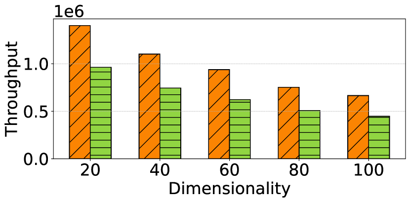
(b) Efficiency

Figure 10: Performance Comparison on Dim workload with varying dimensionality.

5.7 Sensitivity Analysis of Parameters

We conducted an exhaustive sensitivity analysis on two specialized variants of Benne —Benne (Accuracy) and Benne (Efficiency)—utilizing the FCT workload. As previously delineated, Benne (Accuracy) aims for elevated purity levels, while Benne (Efficiency) targets higher throughput rates. Both variants fulfill their respective optimization criteria. We scrutinize the following three parameters:

1) Outlier Distance Threshold ($\delta$): For each data point $x_{t}$ and its nearest cluster $C_{t}$, we compute the distance $D(x_{t},C_{t})$. If this distance surpasses the threshold $\delta$, $x_{t}$ is deemed an outlier. We experimented with $\delta$ values from 50 to 950 for Benne (Accuracy) and from 10 to 100 for Benne (Efficiency). Both variants maintain stable purity and throughput levels across this range. Notably, Benne (Accuracy) undergoes a window model transition from ’landmark’ to ’damped’ when the outlier distance threshold increases within a specific range, causing a sudden alteration in performance metrics. Experimental data indicate an increase in cluster size and purity. However, the throughput does not change, and this is due to the fact that both LandmarkWM and DampedWM are time consuming for clustering. Conversely, Benne (Efficiency) remains unaffected as it does not consider the number of outliers as a performance metric.

2) Queue Size Threshold: We varied the queue size from 20,000 to 100,000. Both variants exhibit a decline in purity as the queue size increases, attributed to less frequent algorithmic adjustments. While the throughput for Benne (Accuracy) diminishes with an increasing queue size due to the growing complexity of its summarizing data structure, Benne (Efficiency) experiences a throughput increase. This is attributed to fewer algorithmic migrations and a transition to a more efficient data structure (Grids) as the queue size enlarges.

3) Variance Threshold: Benne activates the characteristics.frequent evolution flag when the calculated variance of sampled data exceeds a predefined threshold. We tested variance thresholds from 400 to 4,000. As the threshold rises, both purity and throughput for Benne (Accuracy) decline. This is due to the algorithm’s assumption of infrequent evaluations at higher variance thresholds, leading to less frequent algorithmic migrations and increased computational overhead. Benne (Efficiency) remains relatively stable across varying variance thresholds. At a high variance threshold of 4,000, both variants achieve similar purity levels, but Benne (Efficiency) outperforms Benne (Accuracy) in throughput due to the absence of algorithmic migrations.

6 Related Work

This section delineates research contributions pertinent to the four cardinal design aspects of DSC algorithms. These aspects serve as the bedrock for the development of Benne and its automated selection methodology.

Summarizing Data Structure. The quest for efficient data structures for summarizing data streams has been a focal point in research. Zhang et al.[46] introduced the Clustering Feature Tree (CFT), characterized by its incrementality and additivity, making it well-suited for streaming workloads. Aggarwal et al.[16] extended the CF structure into microclusters (MCs), incorporating additional summary information such as timestamps and weights to synergize with window models. Conversely, Chen et al.[15] advocated for a grid-based data structure for efficiency. Gong et al.[2] presented the Dependency Tree (DPT), which strikes a balance between efficiency and accuracy. However, DPT may yield sub-optimal results in handling cluster evolution effectively. These contributions inform Benne’s automated selection of appropriate summarizing data structures.

Window Model. Various window models have been proposed to specify the subset of data streams to be processed. Metwally et al.[39] proposed the landmark window model (LandmarkWM), while Zhou et al.[40] and Borassi et al.[19] introduced the sliding window model (SlidingWM). Cao et al.[41] and Chen et al. [15] presented the damped window model (DampedWM), which retains all data but prioritizes the most recent information by associating varying weights. Benne leverages these foundational works to automatically select the most fitting window model, contingent on user-defined objectives and data stream characteristics.

Outlier Detection Mechanism. Outlier detection is a pivotal design aspect in DSC algorithms. Early contributions like BIRCH [14] included an optional phase for identifying outlier candidates based on object density thresholds. Aggarwal et al.[16] introduced the outlier timer (OutlierD-T) for enhanced outlier identification. Wan et al.[17] further conceptualized the outlier buffer (OutlierD-B) to facilitate the transition between outliers and clustered points. Benne incorporates these mechanisms, enabling automated selection of the most suitable outlier detection strategy based on user objectives and data stream characteristics.

Refinement Strategy. Refinement strategies have been integral to DSC algorithms since Aggarwal et al.[16] introduced the online-offline clustering paradigm. Commonly employed offline clustering algorithms include KMeans [5] and its variants such as Scalable k-means [47] and Singlepass k-means [48]. However, our empirical evaluations suggest that refinement strategies often introduce unnecessary computational overhead. Benne takes these observations into account when automatically selecting the most appropriate refinement strategy, aligned with user objectives and data stream characteristics.

7 Conclusion

This paper has introduced Benne, an innovative DSC algorithm that autonomously selects optimal configurations across four pivotal design aspects, contingent on user-defined objectives and the characteristics of the input data stream. We have conducted a meticulous analysis of these design aspects, encompassing the summarizing data structure, window model, outlier detection mechanism, and refinement strategy. Our empirical evaluations substantiate that Benne surpasses existing state-of-the-art algorithms in both accuracy and efficiency by judiciously selecting the most advantageous combinations of these design aspects. Furthermore, our exhaustive experimental investigations have yielded invaluable insights into the trade-offs inherent in various design aspects of DSC algorithms. These insights serve dual purposes: they assist practitioners in making well-informed choices in the design or selection of DSC algorithms and also lay the groundwork for future scholarly endeavors in this domain.

In addition to our theoretical and experimental contributions, we have encapsulated Benne into a Python library, making it readily accessible for both academic research and practical applications. This library serves as a tool for the community to easily implement, test, and extend our algorithm, thereby fostering further advancements in the field of DSC. As avenues for future research, we intend to extend Benne to accommodate high-dimensional data streams and to investigate more sophisticated techniques for the automated selection of optimal configurations based on data stream attributes. We also plan to explore the integration of advanced machine learning methodologies, such as deep learning and reinforcement learning, to further enhance the accuracy and efficiency of DSC algorithms.

References

- [1] M. Tavallaee, E. Bagheri, W. Lu, and A. A. Ghorbani, “A detailed analysis of the kdd cup 99 data set,” in IEEE Symposium on Computational Intelligence for Security and Defense Applications, 2009, pp. 1–6.
- [2] S. Gong, Y. Zhang, and G. Yu, “Clustering stream data by exploring the evolution of density mountain,” Proc. VLDB Endow., vol. 11, no. 4, p. 393–405, oct 2018. [Online]. Available: https://doi.org/10.1145/3164135.3164136
- [3] K. Namitha and G. S. Kumar., “Concept drift detection in data stream clustering and its application on weather data,” Int. J. Agric. Environ. Inf. Syst., vol. 11, no. 1, pp. 67–85, 2020. [Online]. Available: https://doi.org/10.4018/IJAEIS.2020010104
- [4] F. Cai, N.-A. Le-Khac, and M.-T. Kechadi, “Clustering approaches for financial data analysis,” in Proceedings of the 8th International Conference on Data Mining (DMIN 2012), Las Vegas, NV, USA, 2012, pp. 15–18.
- [5] J. Macqueen, “Some methods for classification and analysis of multivariate observations,” in In 5-th Berkeley Symposium on Mathematical Statistics and Probability, 1967, pp. 281–297.
- [6] S. Lloyd, “Least squares quantization in pcm,” IEEE Transactions on Information Theory, vol. 28, no. 2, pp. 129–137, 1982.
- [7] M. Ester, H.-P. Kriegel, J. Sander, and X. Xu, “A density-based algorithm for discovering clusters in large spatial databases with noise.” AAAI Press, 1996, pp. 226–231.
- [8] M. Masud, J. Gao, L. Khan, J. Han, and B. M. Thuraisingham, “Classification and novel class detection in concept-drifting data streams under time constraints,” IEEE Transactions on Knowledge and Data Engineering, vol. 23, no. 6, pp. 859–874, 2011.
- [9] M. M. Masud, Q. Chen, L. Khan, C. Aggarwal, J. Gao, J. Han, and B. Thuraisingham, “Addressing concept-evolution in concept-drifting data streams,” in 2010 IEEE International Conference on Data Mining, 2010, pp. 929–934.
- [10] A. Haque, L. Khan, M. Baron, B. Thuraisingham, and C. Aggarwal, “Efficient handling of concept drift and concept evolution over stream data,” in 2016 IEEE 32nd International Conference on Data Engineering (ICDE), 2016, pp. 481–492.
- [11] J. Lu and et al., “Learning under concept drift: A review,” IEEE Transactions on Knowledge and Data Engineering, vol. 31, no. 12, pp. 2346–2363, 2019.
- [12] M. Carnein, D. Assenmacher, and H. Trautmann., “An empirical comparison of stream clustering algorithms.” In Proceedings of the Computing Frontiers Conference.(CF’ 17), vol. 17, p. 361–366, 2017.
- [13] S. Mansalis, E. Ntoutsi, N. Pelekis, and Y. Theodoridis, “An evaluation of data stream clustering algorithms,” Statistical Analysis and Data Mining: The ASA Data Science Journal, vol. 11, 06 2018.
- [14] T. Zhang, R. Ramakrishnan, and M. Livny, “Birch: An efficient data clustering method for very large databases,” SIGMOD Rec., vol. 25, no. 2, p. 103–114, jun 1996. [Online]. Available: https://doi.org/10.1145/235968.233324
- [15] Y. Chen and L. Tu, “Density-based clustering for real-time stream data,” in Proceedings of the 13th ACM SIGKDD International Conference on Knowledge Discovery and Data Mining, ser. KDD ’07. New York, NY, USA: Association for Computing Machinery, 2007, p. 133–142.
- [16] C. C. Aggarwal, J. Han, J. Wang, and P. S. Yu, “A framework for clustering evolving data streams,” in Proceedings of the 29th International Conference on Very Large Data Bases - Volume 29, ser. VLDB ’03. VLDB Endowment, 2003, p. 81–92.
- [17] L. Wan, W. K. Ng, X. H. Dang, P. S. Yu, and K. Zhang, “Density-based clustering of data streams at multiple resolutions,” ACM Trans. Knowl. Discov. Data, vol. 3, no. 3, July 2009.
- [18] M. Hahsler and M. Bolaños, “Clustering data streams based on shared density between micro-clusters,” IEEE Transactions on Knowledge and Data Engineering, vol. 28, no. 6, pp. 1449–1461, 2016.
- [19] M. Borassi, A. Epasto, S. Lattanzi, S. Vassilviskii, and M. Zadimoghaddam, “Sliding window algorithms for k-clustering problems,” in Proceedings of the 34th International Conference on Neural Information Processing Systems, ser. NIPS’20. Red Hook, NY, USA: Curran Associates Inc., 2020.
- [20] M. R. Ackermann and et al., “Streamkm++: A clustering algorithm for data streams,” ACM J. Exp. Algorithmics, vol. 17, May 2012.
- [21] A. Bechini and et al., “Tsf-dbscan: a novel fuzzy density-based approach for clustering unbounded data streams,” IEEE Transactions on Fuzzy Systems, 2020.
- [22] D. Barbará, “Requirements for clustering data streams,” ACM SIGKDD Explorations Newsletter, vol. 3, no. 2, p. 23–27, Jan. 2002. [Online]. Available: https://doi.org/10.1145/507515.507519
- [23] J. A. Silva, E. R. Faria, R. C. Barros, E. R. Hruschka, A. C. P. L. F. d. Carvalho, and J. a. Gama, “Data stream clustering: A survey,” ACM Comput. Surv., vol. 46, no. 1, jul 2013. [Online]. Available: https://doi.org/10.1145/2522968.2522981
- [24] X. Wang, Z. Wang, Z. Wu, S. Zhang, X. Shi, and L. Lu, “Data stream clustering: An in-depth empirical study,” Proc. ACM Manag. Data, vol. 1, no. 2, jun 2023. [Online]. Available: https://doi.org/10.1145/3589307
- [25] M. Deepa, P. Revathy, and P. G. Student, “Validation of document clustering based on purity and entropy measures,” 2012.
- [26] H. Kremer and et al., “An effective evaluation measure for clustering on evolving data streams,” in Proceedings of the 11th ACM SIGKDD International Conference on Knowledge Discovery and Data Mining. New York, NY, USA: Association for Computing Machinery, 2011. [Online]. Available: https://doi.org/10.1145/2020408.2020555
- [27] C. C. Aggarwal, Data Streams: Models and Algorithms. Springer Science & Business Media, 2013.
- [28] S. Muthukrishnan, “Data streams: Algorithms and applications,” in Foundations and Trends in Theoretical Computer Science, vol. 1, no. 2. Now Publishers Inc, 2005, pp. 117–236.
- [29] G. Cormode and M. Garofalakis, “Synopses for massive data: Samples, histograms, wavelets, sketches,” Foundations and Trends in Databases, vol. 4, no. 1–3, pp. 1–294, 2012.
- [30] M. M. Gaber, A. Zaslavsky, and S. Krishnaswamy, “Mining data streams: a review,” ACM Sigmod Record, vol. 34, no. 2, pp. 18–26, 2005.
- [31] M. Datar, A. Gionis, P. Indyk, and R. Motwani, “Maintaining stream statistics over sliding windows,” in Proceedings of the thirteenth annual ACM-SIAM symposium on Discrete algorithms. SIAM, 2002, pp. 635–644.
- [32] V. Chandola, A. Banerjee, and V. Kumar, “Anomaly detection: A survey,” ACM computing surveys (CSUR), vol. 41, no. 3, pp. 1–58, 2009.
- [33] C.-T. Lu, D. Chen, and Y. Kou, “Algorithms for spatial outlier detection,” in Third IEEE International Conference on Data Mining. IEEE, 2003, pp. 597–600.
- [34] M. M. Breunig, H.-P. Kriegel, R. T. Ng, and J. Sander, “Lof: identifying density-based local outliers,” in Proceedings of the 2000 ACM SIGMOD international conference on Management of data. ACM, 2000, pp. 93–104.
- [35] H.-P. Kriegel, M. Schubert, and A. Zimek, “Angle-based outlier detection in high-dimensional data,” in Proceedings of the 14th ACM SIGKDD International Conference on Knowledge Discovery and Data Mining, ser. KDD ’08. New York, NY, USA: Association for Computing Machinery, 2008, p. 444–452. [Online]. Available: https://doi.org/10.1145/1401890.1401946
- [36] J. Gama, I. Žliobaitė, A. Bifet, M. Pechenizkiy, and A. Bouchachia, “A survey on concept drift adaptation,” ACM computing surveys (CSUR), vol. 46, no. 4, pp. 1–37, 2014.
- [37] R. Klinkenberg, “Learning drifting concepts: Example selection vs. example weighting,” in Intelligent Data Analysis. Springer, 2004, pp. 281–300.
- [38] J. Gama, P. Medas, G. Castillo, and P. Rodrigues, “Learning with drift detection,” in Brazilian Symposium on Artificial Intelligence. Springer, 2004, pp. 54–64.
- [39] A. Metwally, D. Agrawal, and A. El Abbadi, “Duplicate detection in click streams,” in Proceedings of the 14th international conference on World Wide Web, 2005, pp. 12–21.
- [40] A. Zhou, F. Cao, W. Qian, and C. Jin, “Tracking clusters in evolving data streams over sliding windows,” Knowledge and Information Systems, vol. 15, no. 2, pp. 181–214, 2008.
- [41] F. Cao, M. Estert, W. Qian, and A. Zhou, “Density-based clustering over an evolving data stream with noise,” in Proceedings of the 2006 SIAM international conference on data mining. SIAM, 2006, pp. 328–339.
- [42] Covertype. http://archive.ics.uci.edu/ml/datasets/Covertype.
- [43] V. M. A. Souza, D. M. Reis, A. G. Maletzke, and G. E. A. P. A. Batista, “Challenges in benchmarking stream learning algorithms with real-world data,” Data Mining and Knowledge Discovery, vol. 34, pp. 1805–1858, 2020.
- [44] Sensor. https://www.cse.fau.edu/~xqzhu/stream.html.
- [45] (2021) Moa. [Online]. Available: https://moa.cms.waikato.ac.nz/
- [46] T. Zhang, R. Ramakrishnan, and M. Livny, “Birch: A new data clustering algorithm and its applications,” Data mining and knowledge discovery, vol. 1, no. 2, pp. 141–182, 1997.
- [47] P. Bradley, J. Gehrke, R. Ramakrishnan, and R. Srikant, “Scaling mining algorithms to large databases,” Communications of the ACM, vol. 45, no. 8, pp. 38–43, 2002.
- [48] F. Farnstrom, J. Lewis, and C. Elkan, “Scalability for clustering algorithms revisited,” ACM SIGKDD Explorations Newsletter, vol. 2, no. 1, pp. 51–57, 2000.