Interpreting IV Estimators in Information Provision Experiments

Abstract

A growing literature measures “belief effects” —that is, the causal effect of a change in beliefs on actions— using information provision experiments, where the provision of information is used as an instrument for beliefs. In experimental designs with a passive control group, and under heterogeneous belief effects, we show that the use of information provision as an instrument may not produce a positive weighted average of belief effects. We develop an “information provision instrumental variables” (IPIV) framework that infers the direction of belief updating using information about prior beliefs. In this framework, we propose a class of IPIV estimators that recover positive weighted averages of belief effects. Relative to our preferred IPIV, commonly used specifications in the literature require additional assumptions to generate positive weights. And in the cases where these additional assumptions are satisfied, the identified parameters often up-weight individuals with priors that are further from the provided information, which may not be desirable.

1 Introduction

There is a growing experimental literature that seeks to estimate the causal effects of beliefs on actions. These “belief effects” are relevant for many economic applications. For example, Deshpande and Dizon-Ross, (2023) evaluate the effect of parents’ expectations of government benefits on their investments in human capital for their children, Jäger et al., (2023) evaluate the effect of workers’ beliefs about outside job options on their job search behaviors, Cullen and Perez-Truglia, (2022) evaluate the effect of workers’ beliefs about manager and coworker salaries on their effort, Coibion et al., (2022) evaluate the effect of households’ inflation expectations on their spending decisions, and Roth and Wohlfart, (2020) evaluate the effect of individuals’ recession expectations on their consumption and stock market investments.

These papers estimate belief effects through information provision experiments. Broadly, the literature considers two types of experimental design, a passive control group design and an active control group design. The passive control group design is generally as follows. First, prior beliefs (e.g. one’s expectation of inflation, one’s belief about the salary of their manager) are elicited. Second, subjects are split into a control group and a treatment group. The control group receives no information. The treatment group receives a signal, generally a prediction or measurement of the same quantitative value (eg. an analyst’s inflation forecast, the salary of one’s manager). Then, posterior beliefs are elicited. Finally, participants’ actions are observed (eg. prices set, hours at work). Some papers consider variants of this design with multiple treatment arms, each of which is provided with different information (Coibion et al.,, 2021, 2022; Kumar et al.,, 2023).

The active control group design is the same, except a signal (differing from the signal provided to the treatment group) is also provided to the control group (Akesson et al.,, 2020; Bottan and Perez-Truglia,, 2020; Link et al.,, 2023; Roth et al.,, 2022; Settele,, 2022). For example, Roth and Wohlfart, (2020) provide two different recession forecasts to the treatment and control groups.

In both designs, researchers employ instrumental variables (IV). In particular, the estimation procedure involves a two-stage least squares regression of the action on the posterior belief, where the posterior belief is instrumented by group assignment. The set of instruments may also include interactions of group assignment with the prior, signal, or a combination of the prior and signal. These IV estimators are often interpreted as weighted averages of belief effects.

In settings where causal effects are heterogeneous, the baseline IV estimator generally requires the IV monotonicity condition in order to recover average causal effects with non-negative weights (Imbens and Angrist,, 1994). In active control experiments, monotonicity often seems like a reasonable assumption: it is plausible that individuals who receive a pessimistic signal would conclude a more pessimistic state than had they received an optimistic signal. But in passive control experiments, the monotonicity condition is less plausible. In particular, if individuals update their priors towards the provided signal, then the simultaneous presence of upwards-biased priors and downwards-biased priors (relative to the signal) can generate negative weights.

We propose an information provision instrumental variables (IPIV) framework for estimation in passive control experiments that collect prior beliefs. Our core assumption is that individuals update their prior beliefs towards the provided signals. Given this assumption, we can infer the “direction” in which group assignment affects prior beliefs. In turn, our solution to negative weighting is to augment the standard IV specification with a function that accounts for this inferred direction. The resulting IPIV estimator produces a positive-weighted average of belief effects. This procedure is valid for any number of information provision groups, and so IPIV accommodates settings with multiple treatment arms, such as Coibion et al., (2022).

We use the IPIV framework to analyze existing specifications from passive control experiments. We find that many of these specifications require specific conditions on the values of the first-stage coefficients in order to recover a positive-weighted average of belief effects. Our proposed IPIV estimators are robust to such concerns. In the cases where the existing specifications recover positive-weighted averages, the weights tend to up-weight observations with priors that are further from the signal, which may not be desirable. If such weights are desired, then the IPIV estimator can be generalized to recover these up-weighted parameters, without requiring specific conditions on the first-stage coefficients.

Our IPIV framework is designed for information provision experiments. That said, our recognition of negative weighting in IV estimators is similar in spirit to Blandhol et al., (2022) and Słoczyński, (2022). The former show that linear IV specifications can generate negative weights in settings where the IV assumptions hold conditional on exogenous covariates. In our setting, however, the IV assumptions are unconditional. Słoczyński, (2022) considers a similar setting to Blandhol et al., (2022), and develops a “reordered” IV approach that recovers non-negative weights whenever a “weak monotonicity” condition is satisfied. While our IPIV assumption can be viewed as an instance of weak monotonicity, the availability of data on priors beliefs allows us to exactly distinguish the “compliers” from the “defiers”. In our setting, the endogenous variable is also continuous, which generates additional sources of heterogeneity. The interpretation of IV estimators with continuous endogenous variables is also considered in Angrist et al., (2000), but under the assumption of monotonicity.

This paper proceeds as follows. In Section 2, we provide a model of beliefs, belief effects, and information provision experiments. In Section 3, we motivate and present the IPIV estimator in a general environment. In Section 4, we apply the IPIV framework to common estimators in passive control settings with a single signal. Throughout, we illustrate our results with simulations in a simple setting with Bayesian updating. All proofs are provided in the Appendix.

2 Model

There is an i.i.d. sample of individuals $i=1,\ldots,N$, each with a latent belief probability distribution $F_{i}\in\Delta(\mathcal{Q})$ over a set of states $q\in\mathcal{Q}\subseteq\mathbb{R}$. We observe the action $Y_{i}\in\mathbb{R}$ that individual $i$ takes under $F_{i}$. For example, $F_{i}$ can represent employee $i$’s beliefs on the average earnings of her coworkers, and $Y_{i}$ can be the effort that she exerts when working under these beliefs, as in Cullen and Perez-Truglia, (2022). The goal is to estimate the causal effect of beliefs on actions.

2.1 Beliefs

For each individual, we observe $B_{i}:=\int q\,dF_{i}$, which is a subjective expectation of the state. We suppose that $B_{i}$ is action-relevant in the sense that there is some choice process that maps $b\in\mathbb{R}$ to potential actions $Y_{i}(b)$, where $Y_{i}\equiv Y_{i}(B_{i})$. Because the literature generally elicits only the single expectation $B_{i}$, we simply refer to $B_{i}\in\mathbb{R}$ as “beliefs”, and to $b\in\mathbb{R}$ as “potential beliefs”.

2.2 Target Parameter

In our framework, the effect of a marginal change in beliefs for individual $i$ is $\partial Y_{i}(b)/\partial b$. Therefore, given a weighting function $\omega_{i}(b)$, the average belief effect (ABE) is

$$\theta(\omega):=\mathbb{E}\left[\int\frac{\partial Y_{i}(b)}{\partial b}\omega_{i}(b)\,db\right].$$ (1)

The weighting function $\omega_{i}(b)$ governs the importance of $b$ in the space of potential beliefs, and the importance of $i$ in the distribution of individuals.

2.3 Weighting

In order for $\theta(\omega)$ to be a proper weighted average, we require that $\omega_{i}(b)\geq 0$. Otherwise, the ABE can be misleading. For example, in a setting where all the belief effects are positive, the presence of negative weights can generate a negative ABE. We also require that $\int\mathbb{E}[\omega_{i}(b)]\,db=1$. Together with $\omega_{i}(b)\geq 0$, this condition ensures that the ABE is in the convex hull of the belief effects $\partial Y_{i}(b)/\partial b$.

2.4 Heterogeneity

Our framework places no functional form restrictions on the choice process. In particular, we permit $Y_{i}(b)$ to be a non-parametric function of $b$, which allows for general forms of heterogeneity (Imbens,, 2007). This level of generality is standard practice in applied econometrics.

Given that beliefs are continuous, there are two main sources of heterogeneity (Angrist et al.,, 2000). First, the belief effect $\partial Y_{i}(b)/\partial b$ is generally a nonlinear curve over the space of potential beliefs $b$. In particular, the effect of a marginal change in beliefs depends on the initial belief. The second source of heterogeneity is across individuals. In this general environment, we show that the baseline IV estimator recovers an ABE with weights that can be negative.

In the context of information provision experiments, there is often an implicit recognition of heterogeneity. For example, Cullen and Perez-Truglia, (2022) suggest that their IV estimator recovers meaningful parameters in the presence of heterogeneous effects, and Deshpande and Dizon-Ross, (2023) argue that their IV estimator mitigates the negative weighting issues that can arise from heterogeneous effects. In this paper, we explicitly consider heterogeneity for information provision experiments, and demonstrate its consequences for interpreting IV estimators.

2.5 Covariates

In practice, researchers use baseline covariates $W_{i}$ to improve estimation precision. These covariates are a subset of the control variables $X_{i}$ that are included in a regression specification. For example, we assume that $X_{i}$ contains a constant 1, and so our regressions always include a constant $1$ term. Moreover, numerous specifications in the information provision literature control for pre-determined variables that the information provision experiment generates (see Section 2.6).

2.6 Information Provision

To estimate ABEs, researchers often use information provision experiments. In these experiments, the random assignment to information provision groups $g_{0},\ldots,g_{K}$ generates causal variation in beliefs. If individual $i$ is assigned to group $g_{k}$, then she receives signal $S_{ki}$. For example, in Deshpande and Dizon-Ross, (2023), the state space $\mathcal{Q}=[0,1]$ indexes the probability of receiving government benefits in adulthood, and there is $K=1$ treatment group. In this context, the experiment provides a predicted probability $S_{1i}$ to parents in group $g_{1}$.

In our framework, we suppose that the experiment collects “prior beliefs” $P_{i}:=\int q\,dF_{i}^{P}$ before providing information, where $F_{i}^{P}\in\Delta(\mathcal{Q})$ is a prior distribution. For example, Jäger et al., (2023) collect wage expectations. This collection assumption is essentially without loss of generality, since we are free to consider specifications where $P_{i}$ is not included in the set of control variables $X_{i}$.

We suppose that the groups are distinct in the sense that $g_{\ell}\neq g_{k}$ implies $\mathbb{P}(S_{\ell i}=S_{ki})=0$, which is without loss of generality. In a passive control design, the control group $g_{0}$ does not receive information. For analytical convenience, we set $S_{0i}:=P_{i}$.

The counterfactual beliefs are $B_{ki}:=\int q\,dF_{ki}$, where $F_{ki}\in\Delta(\mathcal{Q})$ depends on the signal $S_{ki}$. Observed beliefs are $B_{i}:=\int q\,dF_{i}$, where

$$B_{i} \equiv\sum_{k=0}^{K}\mathbf{1}(G_{i}=g_{k})B_{ki}, F_{i} \equiv\sum_{k=0}^{K}\mathbf{1}(G_{i}=g_{k})F_{ki}.$$ (2)

Here $G_{i}$ is a random variable that indicates group membership. We sometimes refer to $B_{i}$ and $F_{i}$ as “posterior beliefs”, and to $P_{i}$ and $F_{i}^{P}$ as “prior beliefs”. Notice that the signals are chosen as part of the experimental design, and so $S_{ki}$ is observed for all $g_{k}$.

So far, we are agnostic as to how exactly posteriors depend on the signal and prior, as well as how the signal is drawn; this structure nests the “model averaging” relationship between priors, signals, and posteriors common in this literature (Roth and Wohlfart,, 2020; Cullen and Perez-Truglia,, 2022; Haaland and Roth,, 2023).

Example 1 (Model Averaging).

For each $i$ and $g_{k}$, there exists “learning rate” $\alpha_{ki}\in[0,1]$ such that

$$B_{ki}=\alpha_{ki}S_{ki}+(1-\alpha_{ki})P_{i}.$$ (3)

Example 1 is satisfied, for instance, in certain Bayesian learning models with Gaussian prior distributions $F_{i}^{P}$ and a Gaussian-distributed signal $S_{ki}$ (Hoff,, 2009, Section 5).

2.7 Instrumental Variables

Taking stock, the observed variables in the experiment are $(G_{i},Y_{i},B_{i},S_{ki},P_{i},W_{i})$. We are now prepared to state the core IV assumption.

Assumption 1 (Valid Instrument).

$G_{i}\perp\!\!\!\!\!\!\perp(Y_{i}(b),F_{ki},S_{ki},F_{i}^{P},W_{i})$.

Assumption 1 states that group membership is exogenous. For example, the experiment cannot assign groups based on the values of the covariates. That said, Assumption 1 permits signal structures that are endogenous. For instance, the experiment can use the values of $W_{i}$ to choose the values of $S_{ki}$, as in Deshpande and Dizon-Ross, (2023).

Assumption 1 restricts the effect of group assignment on choices. Indeed, $G_{i}\perp\!\!\!\!\!\!\perp Y_{i}(b)$ means that $G_{i}$ can only impact $Y_{i}\equiv Y_{i}(B_{i})$ through its impact on $B_{i}$. This is the IV exclusion restriction (cf. Angrist and Imbens, (1995)). For example, exclusion fails if choices depend on beliefs that are not collected. In the information provision literature, this concern is known as cross-learning (Haaland and Roth,, 2023). One approach to such concerns is to collect and incorporate a multitude of relevant beliefs into the IV analysis, similar to the approach in Cullen and Perez-Truglia, (2022). We plan to investigate this avenue in future work. Another threat to exclusion is salience: the information provision may increase the salience of a topic, thereby affecting the unobserved components of $Y_{i}(b)$. These salience concerns are beyond the scope of our analysis.

The IV approach also requires that the variation in group assignment generates sufficient variation in beliefs. This is the IV relevance condition. In the context of information provision experiments, this condition often necessitates that some individuals are incorrect in their beliefs, and that these individuals update their beliefs based on the signals. The exact requirements for IV relevance depend on the specification.

For our future identification results, it actually suffices to assume $G_{i}\perp\!\!\!\!\!\!\perp(Y_{i}(b),B_{ki},S_{ki},P_{i},W_{i})$, which is implied by Assumption 1. Nevertheless, the latent belief distribution structure is useful for exploring potential sources of negative weighting (see Section 3.2) and interpreting potential solutions (see Sections 3.4 and 4).

3 IPIV Framework

In this section, we propose a framework for constructing and interpreting IV estimators in information provision experiments. In this analysis, we consider

$$\begin{split}Z_{i}&:=\mathbf{1}(G_{i}\neq g_{0}),\\ \sigma_{\ell k,i}&:=[\mathbf{1}(B_{\ell i}\leq B_{ki})-\mathbf{1}(B_{\ell i}\geq B_{ki})]\mathbf{1}(B_{\ell i}\neq B_{ki}),\\ \mathcal{M}_{\ell k,i}&:=\{B_{\ell i}<b<B_{ki}\}\cup\{B_{\ell i}>b>B_{ki}\}.\end{split}$$ (4)

If $B_{\ell i}\neq B_{ki}$, then $\sigma_{\ell k,i}$ gives the sign of $B_{\ell i}-B_{ki}$. For these individuals, the set $\mathcal{M}_{\ell k,i}$ collects the potential beliefs $b$ that are in between $B_{\ell i}$ and $B_{ki}$. In the program evaluation literature with $K=1$, recall that $\sigma_{01,i}=1$ indicates compliance and $\sigma_{01,i}=-1$ indicates defiance (Angrist et al.,, 1996). For our purposes, we say that $|\sigma_{\ell k,i}|=1$ indicates movement. In particular, $\mathcal{M}_{\ell k,i}$ gives the set of potential beliefs $b$ that individual $i$ moves over when updating from $F_{\ell i}$ to $F_{ki}$, and vice versa.

In numerous applications, we have $K=1$. Therefore, most of our results are stated for the case of $K=1$. However, analogous results are valid for $K>1$, as we demonstrate in Section 3.6.

3.1 Baseline IV

Specification 1 (Baseline IV).

The baseline IV specification is

$$\begin{split}B_{i}&=X_{i}^{\prime}\pi_{0}+\pi_{1}Z_{i}+v_{i},\\ Y_{i}&=X_{i}^{\prime}\gamma_{0}+\gamma_{1}\hat{B}_{i}+e_{i},\end{split}$$ (5)

where $v_{i}$ and $e_{i}$ are regression residuals, $\hat{B}_{i}\equiv X_{i}^{\prime}\pi_{0}+\pi_{1}Z_{i}$ is the first-stage regression, and $\gamma_{1}$ is the coefficient of interest. Let $\tilde{Z}_{i}:=Z_{i}-\mathbb{L}[Z_{i}|X_{i}]$, where $\mathbb{L}[Z_{i}|X_{i}]$ is a regression of $Z_{i}$ on $X_{i}$.

Theorem 1.

Consider Specification 1 for $K=1$. If Assumption 1 is satisfied, $\mathbb{E}[X_{i}X_{i}^{\prime}]$ is full-rank, $\textnormal{var}(\tilde{Z}_{i})>0$, and $\mathbb{E}[\tilde{Z}_{i}B_{i}]\neq 0$, then $\gamma_{1}=\theta(\omega)$ with weighting function

$$\omega_{i}(b)=\cfrac{\sigma_{01,i}\mathbf{1}(b\in\mathcal{M}_{01,i})}{\displaystyle\int\mathbb{E}[\sigma_{01,i}\mathbf{1}(b\in\mathcal{M}_{01,i})]\,db}.$$ (6)

Before we interpret the baseline IV estimator, we first discuss the technical assumptions in Theorem 1. It is worthwhile to have this discussion at least once, since we make similar assumptions in future specifications. To start, the rank condition on $\mathbb{E}[X_{i}X_{i}^{\prime}]$ and $\textnormal{var}(\tilde{Z}_{i})>0$ ensure that the first-stage coefficients are identified. The former requires that there is sufficient variation in the control variables. Given this variation, the latter requires that there remains sufficient variation in group membership. These types of assumptions are straightforward to evaluate in practice, and so we take them as given. The assumption that $\mathbb{E}[\tilde{Z}_{i}B_{i}]\neq 0$ is a sufficient IV relevance condition for Specification 1. The intuition is that the (remaining) variation in group membership generates variation in beliefs.

We now interpret the baseline IV estimator. First, observe that the coefficient of interest recovers an ABE as defined in (1), with weights that depend on the set $\mathcal{M}_{01,i}$. Inspecting the definition of $\mathcal{M}_{01,i}$ in (4), we see that the exogenous group assignment in Assumption 1 generates the counterfactual of moving individuals from latent belief distribution $F_{0i}$ to latent belief distribution $F_{1i}$. The length of this move depends on the impact of the signals. For a given individual $i$, this counterfactual change in beliefs affects choices $Y_{i}(b)$. The ABE summarizes the impact of this change by averaging (integrating) the belief effect curve $\partial Y_{i}(b)/\partial b$ over the set of potential beliefs $b$ that are in between $B_{0i}$ and $B_{1i}$. The ABE then averages this process over all individuals $i$.

Notice that, conditional on the identification of $\gamma_{1}$, the choice of control variables $X_{i}$ does not affect the identified parameter $\theta(\omega)$. This is another consequence of Assumption 1. That said, the choice of control variables may affect the variance of the IV estimator.

3.2 Negative Weighting

The above interpretations are generally valid across IV specifications with continuous endogenous variables (Angrist et al.,, 2000). The core similarity is the presence of $\mathcal{M}_{\ell k,i}$. The point of departure, however, is in the additional components of the ABE weighting function. For example, the weights in Specification 1 are functions of $\sigma_{01,i}$. If some individuals have $\sigma_{01,i}=1$ while others have $\sigma_{01,i}=-1$, then some of these weights will be negative. As noted, the presence of negative weights can produce misleading results. However, if $\sigma_{01,i}\geq 0$ for all $i$, or if $\sigma_{01,i}\leq 0$ for all $i$, then all the weights are non-negative. The latter scenarios are instances where the IV monotonicity condition is satisfied (cf. Angrist et al., (2000)).

The design of the information provision experiment will dictate $\sigma_{01,i}$. In passive control designs, some individuals will have priors that are less than the signal (under-estimators) and some individuals will have priors that are greater than the signal (over-estimators). If we assume that individuals move towards the signal, then under-estimators will have $\sigma_{01,i}=1$ and over-estimators will have $\sigma_{01,i}=-1$, violating monotonicity.

In contrast, in active control designs, as long as $S_{0i}\leq S_{1i}$ implies $B_{0i}\leq B_{1i}$ and $S_{0i}\geq S_{1i}$ implies $B_{0i}\geq B_{1i}$, then monotonicity is satisfied. However, active control designs are not always feasible. There may be settings in which providing two signals may be considered deceptive, or in which there are not two sufficiently different truthful signals to provide enough power. For example, population estimates from any source are likely very similar. In these settings, a passive control design is needed. Furthermore, passive control designs are prevalent in experiments that estimate belief effects (Deshpande and Dizon-Ross,, 2023; Cullen and Perez-Truglia,, 2022; Jäger et al.,, 2023; Coibion et al.,, 2020, 2022). We focus the remainder of the paper on passive control designs.

Consider a passive control baseline IV estimator applied to Example 1. Since $S_{0i}:=P_{i}$, then (3) implies $B_{0i}=P_{i}$. Therefore, $P_{i}\leq S_{ki}$ implies $B_{0i}\leq B_{ki}$, and $P_{i}\geq S_{ki}$ implies $B_{0i}\geq B_{ki}$. For individuals with priors $P_{i}$ that are less than the signal $S_{ki}$ (downward-biased priors), we have $\sigma_{0k,i}\geq 0$. For individuals with priors $P_{i}$ that are greater than the signal $S_{ki}$ (upward-biased priors), we have $\sigma_{0k,i}\leq 0$. Thus, the simultaneous presence of under-estimators and over-estimators violates IV monotonicity. Therefore, in this simple example, the baseline IV estimator produces an ABE that is contaminated by negative weights.

3.3 Simulations

We present simulations of a toy model based on Example 1. For simplicity, instead of heterogeneous learning rates, we use a single homogeneous learning rate $\alpha_{1i}=0.5$ and include additive noise $\varepsilon_{i}$. This toy model satisfies Assumption 1, and the upcoming IPIV Assumption 2. We generate $N=10,000$ observations with parameters as follows. Throughout the rest of the paper, we provide simulated estimates of $\gamma_{1}$ and illustrations of $\omega_{i}(b)$.

$$\begin{split}&P_{i}\sim U[0,10]\\ &S_{1i}=6\\ &Z_{i}\sim\textnormal{Bernoulli}(0.5)\\ &B_{i}=\begin{cases}P_{i}+\varepsilon_{i}&\text{if $Z_{i}=0$}\\ 0.5P_{i}+0.5S_{1i}+\varepsilon_{i}&\text{if $Z_{i}=1$}\end{cases}\\ &Y_{i}(b)=b*P_{i}+\varepsilon_{i},\quad\varepsilon_{i}\sim\textnormal{Normal}(0,1)\end{split}$$ (7)

The belief effect for each individual is $\partial Y_{i}(b)/\partial b=P_{i}$, which is positive and constant over the space of beliefs $b\in\mathbb{R}$. Yet, the baseline IV specification produces -2.41 (s.e. 1.88), a statistically significant negative estimate.

Figure 1 displays the weight $\omega_{i}(b)$ for a given $b$ and prior error $P_{i}-S_{1i}$. There are three values in the plot. The turquoise region has $\omega_{i}(b)=0$, the yellow region has $\omega_{i}(b)=0.0019$, and the purple region has $\omega_{i}(b)=-0.0019$. All individuals with upward-biased priors ($P_{i}-S_{1i}>0$) have negative weights, leading to an overall negative average.

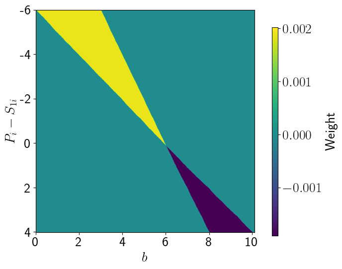
Figure 1: IV weights

3.4 IPIV

In this section, we propose a class of IV specifications for passive control information provision experiments. The goal is to recover an ABE with non-negative weights. Given the results of Specification 1, a natural baseline target is $\theta(\omega)$ with weighting function

$$\omega_{i}(b)=\cfrac{\mathbf{1}(b\in\mathcal{M}_{01,i})}{\displaystyle\int\mathbb{E}[\mathbf{1}(b\in\mathcal{M}_{01,i})]\,db}.$$ (8)

In comparison to the weighting function from Specification 1, there is no contamination from $\sigma_{01,i}$. In particular, while $\omega_{i}(b)$ acknowledges the movement in belief, it remains agnostic to the direction $\sigma_{01,i}$ of this movement.

Assumption 2 (Belief Updating).

$P_{i}\leq S_{ki}$ implies $B_{0i}\leq B_{ki}$ and $P_{i}\geq S_{ki}$ implies $B_{0i}\geq B_{ki}$.

Remark 1 (Testable Implications).

Notice that Assumption 2 is satisfied in Example 1. But even if we do not want to impose the structure from Example 1, we can still test Assumption 2. Indeed, given Assumption 1, $\mathbb{P}(B_{i}\neq P_{i}|G_{i}=g_{0})=\mathbb{P}(B_{0i}\neq P_{i})$. Therefore, if $\mathbb{P}(B_{i}\neq P_{i}|G_{i}=g_{0})=0$, then we can use the observed priors $P_{i}$ as surrogates for the counterfactual $B_{0i}$. In turn,

$$\begin{split}\mathbb{P}(\mathbf{1}(P_{i}\leq S_{ki})\mathbf{1}(P_{i}>B_{i})|G_{i}=g_{k})&=\mathbb{P}(\mathbf{1}(P_{i}\leq S_{ki})\mathbf{1}(P_{i}>B_{ki}))\\ &=\mathbb{P}(\mathbf{1}(P_{i}\leq S_{ki})\mathbf{1}(B_{0i}>B_{ki})).\end{split}$$ (9)

Assumption 2 implies $\mathbb{P}(\mathbf{1}(P_{i}\leq S_{ki})\mathbf{1}(P_{i}>B_{i})|G_{i}=g_{k})=0$, which is a testable implication. Analogously, one can for test whether $P_{i}\geq S_{ki}$ implies $B_{0i}\geq B_{ki}$.

Given Assumption 2, we consider the functions

$$\begin{split}\tilde{\sigma}_{i}:=\sum_{k=1}^{K}[q_{k}\mathbf{1}(G_{i}=g_{0})+\mathbf{1}(G_{i}=g_{k})]\tilde{\sigma}_{0k,i},\quad\quad\tilde{\sigma}_{0k,i}&:=\mathbf{1}(P_{i}\leq S_{ki})-\mathbf{1}(P_{i}\geq S_{ki}),\\ q_{k}&:=\frac{\mathbb{P}(G_{i}=g_{k})}{\mathbb{P}(G_{i}\neq g_{0})}.\end{split}$$ (10)

Lemma 1.

If Assumption 2 is satisfied, then $\tilde{\sigma}_{0k,i}\sigma_{0k,i}=\mathbf{1}(B_{0i}\neq B_{ki})\geq 0$.

Our IPIV approach is to use these functions to correct for negative weighting. Most of our results are stated for $K=1$, since that is the most common setting. In such cases, $\tilde{\sigma}_{i}=\tilde{\sigma}_{01,i}$. That said, IPIV generalizes to $K>1$, as we show in Section 3.6.

Specification 2 (IPIV).

Consider $\lambda_{i}:=\lambda(S_{ki},P_{i},W_{i})\geq 0$ and $\Lambda_{i}(u)=\lambda_{i}\tilde{\sigma}_{i}u$. The IPIV specification is

$$\begin{split}\Lambda_{i}(B_{i})&=X_{i}^{\prime}\pi_{0}+\pi_{1}Z_{i}+v_{i},\\ \Lambda_{i}(Y_{i})&=X_{i}^{\prime}\gamma_{0}+\gamma_{1}\hat{\Lambda}_{i}(B_{i})+e_{i},\end{split}$$ (11)

where $v_{i}$ and $e_{i}$ are regression residuals, $\hat{\Lambda}_{i}(B_{i})\equiv X_{i}^{\prime}\pi_{0}+\pi_{1}Z_{i}$ is the first-stage regression, and $\gamma_{1}$ is the coefficient of interest. Let $\tilde{Z}_{i}:=Z_{i}-\mathbb{L}[Z_{i}|X_{i}]$, where $\mathbb{L}[Z_{i}|X_{i}]$ is a regression of $Z_{i}$ on $X_{i}$.

Theorem 2.

Consider Specification 2 for $K=1$. If Assumptions 1 and 2 are satisfied, $\mathbb{E}[X_{i}X_{i}^{\prime}]$ is full-rank, $\textnormal{var}(\tilde{Z}_{i})>0$, and $\mathbb{E}[\tilde{Z}_{i}\Lambda_{i}(B_{i})]\neq 0$, then $\gamma_{1}=\theta(\omega)$ with weighting function

$$\omega_{i}(b)=\cfrac{\mathbf{1}(b\in\mathcal{M}_{01,i})\lambda_{i}}{\displaystyle\int\mathbb{E}[\mathbf{1}(b\in\mathcal{M}_{01,i})\lambda_{i}]\,db}.$$ (12)

For each $\lambda(S_{ki},P_{i},W_{i})\geq 0$ such that the conditions of Theorem 2 are satisfied, we recover an ABE with convex weights. Notice that $\lambda_{i}$ governs the importance that $\theta(\omega)$ places on individuals with specific values of $(S_{ki},P_{i},W_{i})$. For $\lambda_{i}=1$, the IPIV specification recovers an ABE with weighting function (8). In this case, the ABE places importance in accordance with the joint distribution of $(S_{ki},P_{i},W_{i})$. In Section 4, we show that other choices of $\lambda_{i}$ link our IPIV approach to existing IV specifications that interact group membership with control variables.

Using the simulated data, the IPIV estimate of $\gamma_{1}$ is 3.89 (s.e. 0.276) — a significant positive effect. Figure 2 shows that weights over all individuals and over all beliefs are positive. The positive weights all take the same value. Figure 3 shows that like IV, IPIV has greater weight in regions where more individuals move across a given belief. For example, based on the distribution of priors, more individuals will have $b=3\in[B_{0i},B_{1i}]$ than $b=1\in[B_{0i},B_{1i}]$.

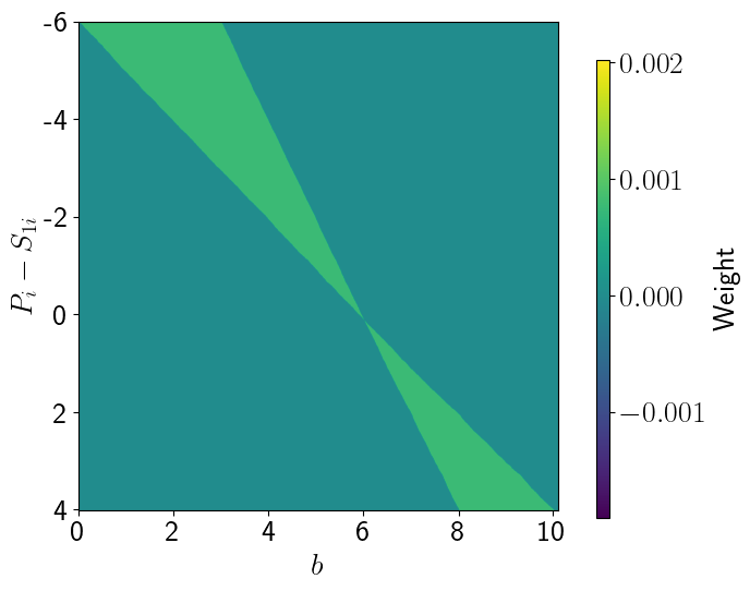
Figure 2: IPIV weights

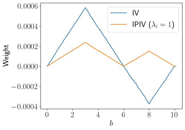
Figure 3: IPIV weights averaged over $i$

3.5 Practical Implications

Assumption 2 is an essential component of Theorem 2. As we noted in Remark 1, this assumption is testable. Furthermore, Assumption 2 has practical consequences for the design of information provision experiments. Notably, it requires that the experiment to collect prior beliefs. This is common practice in many experiments, including Coibion et al., (2022); Deshpande and Dizon-Ross, (2023); Cullen and Perez-Truglia, (2022); Jäger et al., (2023).

Second, Assumption 2 requires that the experiment provides signals for which individuals will update their priors in the direction of those signals. This seems natural in settings where the content of the signal is the same as the content of the priors (e.g. a prior belief for the average coworker wage and a signal of the true average coworker wage, as in Cullen and Perez-Truglia, (2022)). But if the content of the signal is dissimilar to the content of the prior, then Assumption 2 is more tenuous. For example, one of the treatment arms in Coibion et al., (2022) elicits beliefs about the inflation, but provides a signal of recent unemployment. It is less clear how to proceed in such settings.

Assumption 2 is also vulnerable to potential behavioral biases. For example, if some individuals have motivated beliefs or distrust the experimenter, then their priors may update in the “opposite” direction of the signals. We speculate that the testing strategy in Remark 1 would be useful for interrogating such biases.

3.6 IPIV Extensions

There is a natural extension of IPIV to “belief elasticities” $\{b/Y_{i}(b)\}\partial Y_{i}(b)/\partial b$, wherein potential actions $Y_{i}(b)$ and potential beliefs $b$ are positive.

Specification 3 (IPIV in Logs).

Consider $\lambda_{i}:=\lambda(S_{ki},P_{i},W_{i})\geq 0$ and $\Lambda_{i}(u)=\lambda_{i}\tilde{\sigma}_{i}\log(u)$. The IPIV specification in logs is

$$\begin{split}\Lambda_{i}(B_{i})&=X_{i}^{\prime}\pi_{0}+\pi_{1}Z_{i}+v_{i},\\ \Lambda_{i}(Y_{i})&=X_{i}^{\prime}\gamma_{0}+\gamma_{1}\hat{\Lambda}_{i}(B_{i})+e_{i},\end{split}$$ (13)

where $v_{i}$ and $e_{i}$ are regression residuals, $\hat{\Lambda}_{i}(B_{i})\equiv X_{i}^{\prime}\pi_{0}+\pi_{1}Z_{i}$ is the first-stage regression, and $\gamma_{1}$ is the coefficient of interest. Let $\tilde{Z}_{i}:=Z_{i}-\mathbb{L}[Z_{i}|X_{i}]$, where $\mathbb{L}[Z_{i}|X_{i}]$ is a regression of $Z_{i}$ on $X_{i}$.

Theorem 3.

Consider Specification 3 for $K=1$. If Assumptions 1 and 2 are satisfied, $Y_{i}(b),b>0$, $\mathbb{E}[X_{i}X_{i}^{\prime}]$ is full-rank, $\textnormal{var}(\tilde{Z}_{i})>0$, and $\mathbb{E}[\tilde{Z}_{i}\Lambda_{i}(B_{i})]\neq 0$, then $\gamma_{1}=\theta(\omega)$ with weighting function

$$\omega_{i}(b)=\frac{b}{Y_{i}(b)}*\cfrac{b^{-1}\mathbf{1}(b\in\mathcal{M}_{01,i})\lambda_{i}}{\displaystyle\int b^{-1}\mathbb{E}[\mathbf{1}(b\in\mathcal{M}_{01,i})\lambda_{i}]\,db}.$$ (14)

In Theorem 3, the weighting function satisfies $\int\mathbb{E}[\{b/Y_{i}(b)\}^{-1}\omega_{i}(b)]\,db=1$, which is appropriate for settings with belief elasticities. In particular,

$$\theta(\omega)=\mathbb{E}\left[\int\frac{b}{Y_{i}(b)}\frac{\partial Y_{i}(b)}{\partial b}\check{\omega}_{i}(b)\,db\right],\quad\check{\omega}_{i}(b):=\cfrac{b^{-1}\mathbf{1}(b\in\mathcal{M}_{01,i})\lambda_{i}}{\displaystyle\int b^{-1}\mathbb{E}[\mathbf{1}(b\in\mathcal{M}_{01,i})\lambda_{i}]\,db},$$ (15)

where $\check{\omega}_{i}(b)\equiv\{b/Y_{i}(b)\}^{-1}\omega_{i}(b)$ gives convex weights. In such cases, the parameter $\theta(\omega)$ is unit-free, which facilitates comparisons across applications. For a related discussion, see Haaland and Roth, (2023, Section 8).

IPIV accommodates settings where $K>1$, such as Coibion et al., (2021), Coibion et al., (2022), Kumar et al., (2023), and others.

Theorem 4.

Consider Specification 2. If Assumptions 1 and 2 are satisfied, $\mathbb{E}[X_{i}X_{i}^{\prime}]$ is full-rank, $\textnormal{var}(\tilde{Z}_{i})>0$, and $\mathbb{E}[\tilde{Z}_{i}\Lambda_{i}(B_{i})]\neq 0$, then $\gamma_{1}=\theta(\omega)$ with weighting function

$$\omega_{i}(b)=\cfrac{\displaystyle\sum_{k=1}^{K}q_{k}\mathbf{1}(b\in\mathcal{M}_{0k,i})\lambda_{i}}{\displaystyle\sum_{k=1}^{K}q_{k}\int\mathbb{E}[\mathbf{1}(b\in\mathcal{M}_{0k,i})\lambda_{i}]\,db}.$$ (16)

Theorem 4 shows that Specification 2 is valid for $K>1$. In particular, we now recover a convex average of group specific ABEs. Indeed, we have

$$\gamma_{1}=\sum_{k=1}^{K}\psi_{k}\theta(\omega_{k}),\quad\omega_{ki}(b) =\cfrac{\mathbf{1}(b\in\mathcal{M}_{0k,i})\lambda_{i}}{\displaystyle\int\mathbb{E}[\mathbf{1}(b\in\mathcal{M}_{0k,i})\lambda_{i}]\,db},\quad\psi_{k}:=\cfrac{\displaystyle q_{k}\int\mathbb{E}[\mathbf{1}(b\in\mathcal{M}_{0k,i})\lambda_{i}]\,db}{\displaystyle\sum_{k=1}^{K}q_{k}\int\mathbb{E}[\mathbf{1}(b\in\mathcal{M}_{0k,i})\lambda_{i}]\,db}.$$ (17)

For each $\theta(\omega_{k})$, the counterfactual comparison for individual $i$ is between her posterior beliefs when assigned to group $g_{0}$ versus group $g_{k}$.

4 Linking IPIV to Existing Specifications

Our IPIV approach is related to existing specifications that interact group membership with control variables. For each of these specifications, there are conditions on the first-stage coefficients such that IPIV with some function $\lambda_{i}:=\lambda(S_{ki},P_{i},W_{i})$ estimates the same ABE. We give results for these various specifications, along with practical suggestions.

4.1 Prior and Signal Interactions

Specification 4 (Prior and Signal Interactions).

This specification, as in Deshpande and Dizon-Ross, (2023, Section 4), takes the form

$$\begin{split}B_{i}&=X_{i}^{\prime}\pi_{0}+\pi_{1}Z_{i}+\pi_{2}Z_{i}P_{i}+\pi_{3}Z_{i}S_{1i}+v_{i},\\ Y_{i}&=X_{i}^{\prime}\gamma_{0}+\gamma_{1}\hat{B}_{i}+e_{i},\end{split}$$ (18)

where $v_{i}$ and $e_{i}$ are regression residuals, $\hat{B}_{i}\equiv X_{i}^{\prime}\pi_{0}+\pi_{1}Z_{i}+\pi_{2}Z_{i}P_{i}+\pi_{3}Z_{i}S_{1i}$ is the first-stage regression, and $\gamma_{1}$ is the coefficient of interest. Denote $m_{i}(Z_{i}):=(Z_{i},Z_{i}P_{i},Z_{i}S_{1i})^{\prime}$ and $\tilde{m}_{i}(Z_{i})=m_{i}(Z_{i})-\mathbb{L}[m_{i}(Z_{i})|X_{i}]$, where $\mathbb{L}[m_{i}(Z_{i})|X_{i}]$ is a regression of $m_{i}(Z_{i})$ on $X_{i}$.

Theorem 5.

Consider Specification 4 for $K=1$. If Assumption 1 is satisfied, $P_{i}$ and $S_{1i}$ are included in the set of control variables $X_{i}$, $\mathbb{E}[X_{i}X_{i}^{\prime}]$ and $\mathbb{E}[\tilde{m}_{i}(Z_{i})\tilde{m}_{i}(Z_{i})^{\prime}]$ are full-rank, and $\mathbb{E}[\tilde{m}_{i}(Z_{i})B_{i}]\neq 0$, then $\gamma_{1}=\theta(\omega)$ with weighting function

$$\omega_{i}(b)=\cfrac{\sigma_{01,i}\mathbf{1}(b\in\mathcal{M}_{01,i})(\pi_{1}+\pi_{2}P_{i}+\pi_{3}S_{1i})}{\displaystyle\int\mathbb{E}[\sigma_{01,i}\mathbf{1}(b\in\mathcal{M}_{01,i})(\pi_{1}+\pi_{2}P_{i}+\pi_{3}S_{1i})]\,db}.$$ (19)

Moreover, if Assumption 2 is satisfied, $\pi_{1}=0$, and $\pi_{2}=-\pi_{3}$, then

$$\omega_{i}(b)=\cfrac{\mathbf{1}(b\in\mathcal{M}_{01,i})\lambda_{i}}{\displaystyle\int\mathbb{E}[\mathbf{1}(b\in\mathcal{M}_{01,i})\lambda_{i}]\,db},\quad\lambda_{i}=|S_{1i}-P_{i}|.$$ (20)

Theorem 5 shows that Specification 4 recovers an ABE with non-negative weights, provided that $\pi_{1}=0$ and $\pi_{2}=-\pi_{3}$. If the first-stage coefficients attain these values, then Specification 4 recovers an IPIV parameter with $\lambda_{i}=|S_{1i}-P_{i}|$. This means that individuals with larger “prior errors” in their beliefs are up-weighted relative to their share in the distribution of individuals. If we have reason to put greater focus on the actions of “misinformed” individuals, then this up-weighting feature is appealing.

One can compute the first stage and inspect whether the sufficient condition for Specification 4 of $\pi_{1}=0$ and $\pi_{2}=-\pi_{3}$ is satisfied. One setting where the first-stage coefficients attain these is Example 1, with $\alpha_{ki}$ independent of priors and signals.

Theorem 6.

In the context of Example 1, consider the first-stage in Specification 4 for $K=1$. If Assumption 1 is satisfied, $X_{i}=(1,P_{i},S_{1i})^{\prime}$, $\mathbb{E}[X_{i}X_{i}^{\prime}]$ and $\mathbb{E}[\tilde{m}_{i}(Z_{i})\tilde{m}_{i}(Z_{i})^{\prime}]$ are full-rank, and $\alpha_{1i}\perp\!\!\!\!\!\!\perp(F_{i}^{P},S_{1i})$, then the first-stage coefficients are identified such that $\pi_{1}=0$ and $\pi_{2}=-\pi_{3}$.

That said, in general settings, it seems implausible that $\alpha_{ki}$ would be independent of priors and signals. For example, if there is individual heterogeneity across prior distributions $F_{i}^{P}$, and $\alpha_{ki}$ depends on the variance induced by $F_{i}^{P}$, then $P_{i}:=\int q\,dF_{i}^{P}$ is likely correlated with $\alpha_{ki}$. Moreover, it seems that the inclusion of covariates $W_{i}$ would complicate the designation of primitive conditions for $\pi_{1}=0$ and $\pi_{2}=-\pi_{3}$. Given these various concerns, we caution against using Specification 4. Instead, if the goal is an ABE with weighting function (20), then we recommend using IPIV with $\lambda_{i}=|S_{1i}-P_{i}|$.

4.2 Prior Error Interaction

Specification 5 (Prior Error Interaction in Logs).

This specification, as in Jäger et al., (2023, Section 4.4), takes the form

$$\begin{split}\log(B_{i})&=X_{i}^{\prime}\pi_{0}+\pi_{1}Z_{i}+\pi_{2}Z_{i}\log(P_{i}/S_{1i})+v_{i},\\ \log(Y_{i})&=X_{i}^{\prime}\gamma_{0}+\gamma_{1}\textnormal{l}\widehat{\textnormal{og}}(B_{i})+e_{i},\end{split}$$ (21)

where $v_{i}$ and $e_{i}$ are regression residuals, $\textnormal{l}\widehat{\textnormal{og}}(B_{i})\equiv X_{i}^{\prime}\pi_{0}+\pi_{1}Z_{i}+\pi_{2}Z_{i}\log(P_{i}/S_{1i})$ is the first-stage regression, and $\gamma_{1}$ is the coefficient of interest. Let $m_{i}(Z_{i}):=(Z_{i},Z_{i}\log(P_{i}/S_{1i}))^{\prime}$ and $\tilde{m}_{i}(Z_{i})=m_{i}(Z_{i})-\mathbb{L}[m_{i}(Z_{i})|X_{i}]$, where $\mathbb{L}[m_{i}(Z_{i})|X_{i}]$ is a regression of $m_{i}(Z_{i})$ on $X_{i}$.

Theorem 7.

Consider Specification 5 for $K=1$. If Assumption 1 is satisfied, $\log(P_{i}/S_{1i})$ is included in $X_{i}$, $\mathbb{E}[X_{i}X_{i}^{\prime}]$ and $\mathbb{E}[\tilde{m}_{i}(Z_{i})\tilde{m}_{i}(Z_{i})^{\prime}]$ are full-rank, and $\mathbb{E}[\tilde{m}_{i}(Z_{i})\log(B_{i})]\neq 0$, then $\gamma_{1}=\theta(\omega)$ with weighting function

$$\omega_{i}(b)=\frac{b}{Y_{i}(b)}*\cfrac{b^{-1}\sigma_{01,i}\mathbf{1}(b\in\mathcal{M}_{01,i})(\pi_{1}+\pi_{2}\log(P_{i}/S_{1i}))}{\displaystyle\int b^{-1}\mathbb{E}[\sigma_{01,i}\mathbf{1}(b\in\mathcal{M}_{01,i})(\pi_{1}+\pi_{2}\log(P_{i}/S_{1i}))]\,db}.$$ (22)

Moreover, if Assumption 2 is satisfied and $\pi_{1}=0$, then

$$\omega_{i}(b)=\frac{b}{Y_{i}(b)}*\cfrac{b^{-1}\mathbf{1}(b\in\mathcal{M}_{01,i})\lambda_{i}}{\displaystyle\int b^{-1}\mathbb{E}[\mathbf{1}(b\in\mathcal{M}_{01,i})\lambda_{i}]\,db},\quad\lambda_{i}=|\log(P_{i}/S_{1i})|.$$ (23)

Theorem 7 shows that Specification 5 recovers an ABE with non-negative weights, provided that $\pi_{1}=0$. In particular, if $\pi_{1}=0$, then

$$\theta(\omega)=\mathbb{E}\left[\int\frac{b}{Y_{i}(b)}\frac{\partial Y_{i}(b)}{\partial b}\check{\omega}_{i}(b)\,db\right],\quad\check{\omega}_{i}(b):=\cfrac{b^{-1}\mathbf{1}(b\in\mathcal{M}_{01,i})|\log(P_{i}/S_{1i})|}{\displaystyle\int b^{-1}\mathbb{E}[\mathbf{1}(b\in\mathcal{M}_{01,i})|\log(P_{i}/S_{1i})|]\,db}.$$ (24)

The interpretation for the identified $\theta(\omega)$ mirrors the interpretation from Specification 4. In particular, the above ABE up-weights individuals with larger “prior errors”. More importantly, the non-negative weighting result in Theorem 7 requires that $\pi_{1}=0$. Thus, for reasons similar to the ones given for Specification 4, we caution against using Specification 5. Instead, if the goal is an ABE with weighting function (24), then we recommend using IPIV. In particular, Specification 3 with $\lambda_{i}=|\log(P_{i}/S_{1i})|$ generates an ABE with weighting function (24).

4.3 Prior Error Pure Interaction

Specification 6 (Prior Error Pure Interaction in Logs).

This specification takes the form

$$\begin{split}\log(B_{i})&=X_{i}^{\prime}\pi_{0}+\pi_{1}Z_{i}\log(S_{1i}/P_{i})+v_{i},\\ \log(Y_{i})&=X_{i}^{\prime}\gamma_{0}+\gamma_{1}\textnormal{l}\widehat{\textnormal{og}}(B_{i})+e_{i},\end{split}$$ (25)

where $v_{i}$ and $e_{i}$ are regression residuals, $\textnormal{l}\widehat{\textnormal{og}}(B_{i})\equiv X_{i}^{\prime}\pi_{0}+\pi_{1}Z_{i}\log(S_{1i}/P_{i})$ is the first-stage regression, and $\gamma_{1}$ is the coefficient of interest. In contrast to Specification 5, notice that there is no linear term for $Z_{i}$. In that sense, the above first-stage is a “pure interaction” specification. This pure interaction specification is analogous to specifications from Cullen and Perez-Truglia, (2022, Section 4) and Galashin et al., (2020, Section 6), which consider $B_{i}\in\mathbb{R}^{2}$. Let $m_{i}(Z_{i}):=Z_{i}\log(S_{1i}/P_{i})$ and $\tilde{m}_{i}(Z_{i})=m_{i}(Z_{i})-\mathbb{L}[m_{i}(Z_{i})|X_{i}]$, where $\mathbb{L}[m_{i}(Z_{i})|X_{i}]$ is a regression of $m_{i}(Z_{i})$ on $X_{i}$.

Theorem 8.

Consider Specification 6 for $K=1$. If Assumption 1 is satisfied, $\log(S_{1i}/P_{i})$ is included in the set of control variables $X_{i}$, $\mathbb{E}[X_{i}X_{i}^{\prime}]$ is full-rank, $\textnormal{var}(\tilde{m}_{i}(Z_{i}))>0$, and $\mathbb{E}[\tilde{m}_{i}(Z_{i})\log(B_{i})]\neq 0$, then $\gamma_{1}=\theta(\omega)$ with weighting function

$$\omega_{i}(b)=\frac{b}{Y_{i}(b)}*\cfrac{b^{-1}\sigma_{01,i}\mathbf{1}(b\in\mathcal{M}_{01,i})\log(S_{1i}/P_{i})}{\displaystyle\int b^{-1}\mathbb{E}[\sigma_{01,i}\mathbf{1}(b\in\mathcal{M}_{01,i})\log(S_{1i}/P_{i})]\,db}.$$ (26)

Moreover, if Assumption 2 is satisfied, then

$$\omega_{i}(b)=\frac{b}{Y_{i}(b)}*\cfrac{b^{-1}\mathbf{1}(b\in\mathcal{M}_{01,i})\lambda_{i}}{\displaystyle\int b^{-1}\mathbb{E}[\mathbf{1}(b\in\mathcal{M}_{01,i})\lambda_{i}]\,db},\quad\lambda_{i}=|\log(S_{1i}/P_{i})|.$$ (27)

Theorem 8 shows that Specification 6 recovers $\theta(\omega)$ with non-negative weights. Notably, this non-negative weighting result is agnostic to values of the first-stage coefficients, in contrast to the results for Specification 5. This difference arises because Specification 5 includes a linear term for $Z_{i}$.

Therefore, a researcher can use Specification 6 to recover

$$\theta(\omega)=\mathbb{E}\left[\int\frac{b}{Y_{i}(b)}\frac{\partial Y_{i}(b)}{\partial b}\check{\omega}_{i}(b)\,db\right],\quad\check{\omega}_{i}(b):=\cfrac{b^{-1}\mathbf{1}(b\in\mathcal{M}_{01,i})|\log(S_{1i}/P_{i})|}{\displaystyle\int b^{-1}\mathbb{E}[\mathbf{1}(b\in\mathcal{M}_{01,i})|\log(S_{1i}/P_{i})|]\,db},$$ (28)

without needing to be concerned about the values of the first-stage coefficients. Once again, individuals with larger “prior errors” are up-weighted. Theorem 8 supports the interpretation of weights that Cullen and Perez-Truglia, (2022, Section 4) provide for their two-belief analogue of Specification 6.

Given that IPIV Specification 3 with $\lambda_{i}=|\log(S_{1i}/P_{i})|$ and Specification 6 both recover (28), a natural question is whether one procedure is more efficient than the other. We plan to investigate this in future work.

4.4 Prior Interaction

Specification 7 (Prior Interaction).

This specification takes the form

$$\begin{split}B_{i}&=X_{i}^{\prime}\pi_{0}+\pi_{1}Z_{i}+\pi_{2}Z_{i}P_{i}+v_{i},\\ Y_{i}&=X_{i}^{\prime}\gamma_{0}+\gamma_{1}\hat{B}_{i}+e_{i},\end{split}$$ (29)

where $v_{i}$ and $e_{i}$ are regression residuals, $\hat{B}_{i}\equiv X_{i}^{\prime}\pi_{0}+\pi_{1}Z_{i}+\pi_{2}Z_{i}P_{i}$ is the first-stage regression, and $\gamma_{1}$ is the coefficient of interest. This prior interaction specification is analogous to specifications from (Coibion et al.,, 2022, Sections 3 and 5), Coibion et al., (2021, Sections 3 and 4), and (Kumar et al.,, 2023, Sections 3 and 4), which consider $K>1$. The latter two also consider $B_{i}\in\mathbb{R}^{2}$. Let $m_{i}(Z_{i}):=(Z_{i},Z_{i}P_{i})^{\prime}$ and $\tilde{m}_{i}(Z_{i})=m_{i}(Z_{i})-\mathbb{L}[m_{i}(Z_{i})|X_{i}]$, where $\mathbb{L}[m_{i}(Z_{i})|X_{i}]$ is a regression of $m_{i}(Z_{i})$ on $X_{i}$.

Theorem 9.

Consider Specification 7 for $K=1$. If Assumption 1 is satisfied, $P_{i}$ is included in the set of control variables $X_{i}$, $\mathbb{E}[X_{i}X_{i}^{\prime}]$ and $\mathbb{E}[\tilde{m}_{i}(Z_{i})\tilde{m}_{i}(Z_{i})^{\prime}]$ are full-rank, and $\mathbb{E}[\tilde{m}_{i}(Z_{i})B_{i}]\neq 0$, then $\gamma_{1}=\theta(\omega)$ with weighting function

$$\omega_{i}(b)=\cfrac{\sigma_{01,i}\mathbf{1}(b\in\mathcal{M}_{01,i})(\pi_{1}+\pi_{2}P_{i})}{\displaystyle\int\mathbb{E}[\sigma_{01,i}\mathbf{1}(b\in\mathcal{M}_{01,i})(\pi_{1}+\pi_{2}P_{i})]\,db}.$$ (30)

Moreover, if Assumption 2 is satisfied, $\pi_{1}=0$, and either (i) $P_{i}\leq 0$ implies $P_{i}\leq S_{1i}$ and $P_{i}\geq 0$ implies $P_{i}\geq S_{1i}$; or (ii) $P_{i}\leq 0$ implies $P_{i}\geq S_{1i}$ and $P_{i}\geq 0$ implies $P_{i}\leq S_{1i}$, then

$$\omega_{i}(b)=\cfrac{\mathbf{1}(b\in\mathcal{M}_{01,i})\lambda_{i}}{\displaystyle\int\mathbb{E}[\mathbf{1}(b\in\mathcal{M}_{01,i})\lambda_{i}]\,db},\quad\lambda_{i}=|P_{i}|.$$ (31)

Theorem 9 shows that Specification 7 recovers an ABE with non-negative weights, provided that $\pi_{1}=0$ and the signals are chosen dependent on the sign of the prior. For example, if a firm believes that inflation will be positive, then the experiment must provide that firm with a signal that is less than the prior. It seems difficult to imagine situations where such signal structures would be desirable; in fact, if only a single signal is provided, this implies that the signal must be smaller than all priors. And of course, the constraint that $\pi_{1}=0$ means that Specification 7 suffers from the same weaknesses as Specifications 4 and 5.

If all assumptions for Specification 4 are satisfied, we recover an IPIV parameter with $\lambda_{i}=|P_{i}|$. This means that individuals with large priors (in magnitude) are up-weighted relative to their share in the distribution of individuals. The value of such a weighting scheme depends on the context. That said, due to the implausibility of the assumptions, if (31) is indeed the target parameter, then we recommend using IPIV Specification 2 with $\lambda_{i}=|P_{i}|$.

4.5 Implications for Estimation and Interpretation

We have shown that Specification 6 provides a positive weighted average over belief effects without assumptions beyond those for IPIV. We have also provided sufficient conditions for Specifications 4, 5, and 7. These sufficient conditions are easily testable by examining the coefficients in the first stage regression. However, based on the stringency of these assumptions, we recommend researchers directly use IPIV with the corresponding $\lambda_{i}$ instead.

Additionally, we have shown that interacting group status with prior beliefs and/or the signal results in an weight $\lambda_{i}$ that generally up-weights individuals whose priors are far from the signal (large prior error) and down-weights individuals whose priors are close to the signal (small prior error). This may lead to especially different estimates if the prior error is correlated with the belief effect. For example, consider a case in which individuals who have the largest belief effects have the greatest demand for information, and therefore have priors that are already close to the signal. Then, these specifications would underweight these individuals, leading the estimated ABE to be attenuated. We believe that using IPIV with $\lambda_{i}=1$ provides a more “natural” object of interest.

Using the simulated data, Table 1 displays estimates of $\gamma_{1}$ under the different specifications. To allow for comparison across estimates, we interact with $P_{i}-S_{1i}$, rather than $\log(P_{i}/S_{1i})$, in Specifications 5 and 6. Note that for regressions 4, 5, and 6, the data is generated such that sufficient conditions for the specifications to produce IPIV estimates are met. Therefore, these regressions provide $\lambda_{i}=|S_{1i}-P_{i}|$ IPIV estimates. The estimates are attenuated relative to the IPIV due to over-weighting of those who have large prior errors and under-weighting of those who have small prior errors. The final regression does not satisfy the sufficient assumption for the relationship between $P_{i}$ and $S_{1i}$ for an IPIV interpretation.

Figure 4 shows the weights plotted over $b$ and $P_{i}-S_{1i}$. There is a gradient towards the center of the figure as the weights shrink. Figure 5 shows a histogram of weights under the Baseline IV, IPIV ($\lambda_{i}=1$), and IPIV ($\lambda_{i}=|P_{i}-S_{1i}|$) specifications. Relative to IPIV ($\lambda_{i}=1$), IPIV ($\lambda_{i}=|P_{i}-S_{1i}|$) has a concentration of weights near 0 and a long right tail. Notice in Figure 6 that the weights near 0 correspond to the points near $P_{i}-S_{1i}=0$. The long tail corresponds to the far left and far right of $P_{i}-S_{1i}$.

Table 1: Estimates of $\gamma_{1}$

	Baseline IV (1)	IPIV (2)	(4)	(5*)	(6*)	(7)
$\gamma_{1}$	-2.410	3.894	3.140	3.124	3.139	3.043
	(1.188)	(0.276)	(0.092)	(0.092)	(0.092)	(0.108)

• Note: The data are simulated as specified in Section 3.3. Standard errors in parentheses. Column headers reference the specification estimated. * indicates that the in-text specification is in logs, but the estimation is in levels.

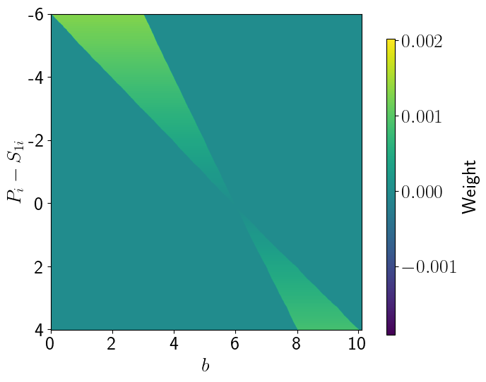
Figure 4: IPIV weights with $\lambda_{i}=|P_{i}-S_{1i}|$

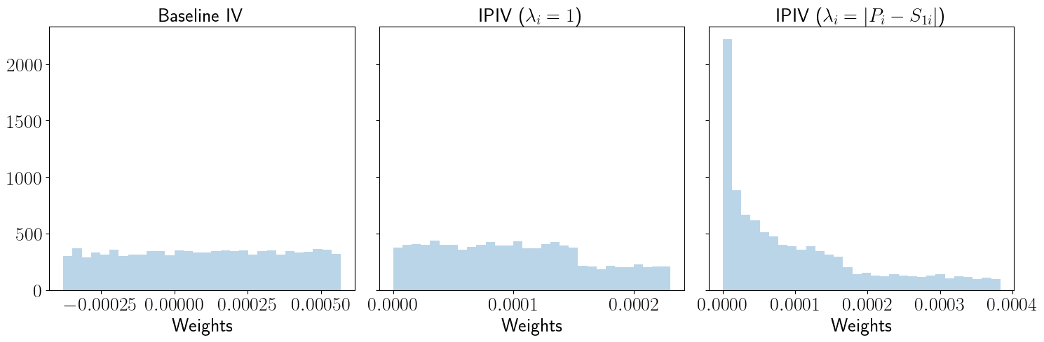
Figure 5: Histogram of weights

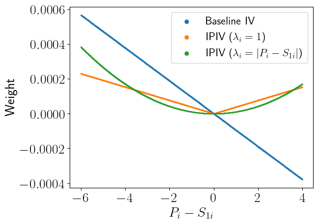
Figure 6: Weights averaged over $b$

5 Conclusion

In this paper, we focus on the identification of the causal effects of beliefs on individuals’ actions in passive control information provision experiments. Within this domain, due to non-monotonicity, a baseline IV regression will generally produce negative weights. We introduce a family of information provision instrumental variables (IPIV) estimators to correct for this issue.

Our framework requires the experiment to obtain prior beliefs and assumes that individuals update their beliefs in the direction of the signal. With this information, we can identify over-and under-estimators, providing a natural correction for non-monotonicity. Like IV, IPIV is dependent on individuals’ beliefs being “moved” by the information provision. Therefore, when designing information provision experiments, researchers should be sure to collect priors and to design meaningful signals that induce predictable variation.

Additionally, we show that many existing specifications in fact produce a weighted form of IPIV. A specification based on that of Cullen and Perez-Truglia, (2022) does so without additional assumptions; specifications from Jäger et al., (2023) and Deshpande and Dizon-Ross, (2023) do so with additional testable conditions on the first stage. However, the weights, relative to IPIV, up-weight individuals with large prior errors and down-weight individuals with small prior errors, which may be undesirable. Similarly, a specification based on Coibion et al., (2022) requires additional assumptions and up-weights individuals with large priors. We illustrate the impacts of these differences in simulated data.

6 Appendix

Proof of Lemma 1.

Assumption 2 implies $\mathbf{1}(P_{i}\leq S_{ki})=\mathbf{1}(P_{i}\leq S_{ki})\mathbf{1}(B_{0i}\leq B_{ki})$ and $\mathbf{1}(P_{i}\geq S_{ki})=\mathbf{1}(P_{i}\geq S_{ki})\mathbf{1}(B_{0i}\geq B_{ki})$. Therefore,

$$\tilde{\sigma}_{0k,i}\sigma_{0k,i} =[\mathbf{1}(P_{i}\leq S_{ki})\mathbf{1}(B_{0i}\leq B_{ki})-\mathbf{1}(P_{i}\leq S_{ki})\mathbf{1}(B_{0i}\geq B_{ki})]\mathbf{1}(B_{0i}\neq B_{ki})$$

$$-[\mathbf{1}(P_{i}\geq S_{ki})\mathbf{1}(B_{0i}\leq B_{ki})-\mathbf{1}(P_{i}\geq S_{ki})\mathbf{1}(B_{0i}\geq B_{ki})]\mathbf{1}(B_{0i}\neq B_{ki})$$

$$=[\mathbf{1}(P_{i}\leq S_{ki})\mathbf{1}(B_{0i}\leq B_{ki})+\mathbf{1}(P_{i}\geq S_{ki})\mathbf{1}(B_{0i}\geq B_{ki})]\mathbf{1}(B_{0i}\neq B_{ki})$$

$$=[\mathbf{1}(P_{i}\leq S_{ki})+\mathbf{1}(P_{i}\geq S_{ki})]\mathbf{1}(B_{0i}\neq B_{ki})$$

$$=\mathbf{1}(B_{0i}\neq B_{ki}).$$

∎

Lemma 2.

If $f_{i}(b)$ is a differentiable function, then

$$f_{i}(B_{\ell i})-f_{i}(B_{ki})=\int\frac{\partial f_{i}(b)}{\partial b}\sigma_{\ell k,i}\mathbf{1}(b\in\mathcal{M}_{\ell k,i})\,db,$$ (32)

where $\sigma_{\ell k,i}:=[\mathbf{1}(B_{\ell i}\leq B_{ki})-\mathbf{1}(B_{\ell i}\geq B_{ki})]\mathbf{1}(B_{\ell i}\neq B_{ki})$ and $\mathcal{M}_{\ell k,i}:=\{B_{\ell i}<b<B_{ki}\}\cup\{B_{\ell i}>b>B_{ki}\}$.

Proof of Lemma 2.

Since $f_{i}(b)$ is differentiable, then the second fundamental theorem of calculus gives

$$f_{i}(B_{\ell i})-f_{i}(B_{ki}) =(f_{i}(B_{\ell i})-f_{i}(B_{ki}))\mathbf{1}(B_{\ell i}\neq B_{ki})$$

$$=\mathbf{1}(B_{\ell i}\leq B_{ki})\int\frac{\partial f_{i}(b)}{\partial b}\mathbf{1}(B_{\ell i}\neq B_{ki})\mathbf{1}(B_{\ell i}<b<B_{ki})\,db$$

$$-\mathbf{1}(B_{\ell i}\geq B_{ki})\int\frac{\partial f_{i}(b)}{\partial b}\mathbf{1}(B_{\ell i}\neq B_{ki})\mathbf{1}(B_{\ell i}>b>B_{ki})\,db.$$

For the first term, notice that $\mathbf{1}(B_{\ell i}\leq B_{ki})\mathbf{1}(B_{\ell i}\neq B_{ki})\mathbf{1}(B_{\ell i}<b<B_{ki})=\mathbf{1}(B_{\ell i}\leq B_{ki})\mathbf{1}(B_{\ell i}\neq B_{ki})\mathbf{1}(b\in\mathcal{M}_{\ell k,i})$. The second term is similar. Therefore, combining terms gives the conclusion. ∎

Lemma 3.

For $\Lambda_{i}:\mathbb{R}\to\mathbb{R}$ and $m_{i}(Z_{i}):=(m_{1i}(Z_{i}),\ldots,m_{Ji}(Z_{i}))^{\prime}$, where $m_{ji}(Z_{i}):=Z_{i}h_{ji}$ and $h_{ji}:=h_{j}(S_{ki},P_{i},W_{i})$. Consider the specification

$$\Lambda_{i}(B_{i}) =X_{i}^{\prime}\pi_{0}+\sum_{j=1}^{J}\pi_{j}m_{ji}(Z_{i})+v_{i},$$

$$\Lambda_{i}(Y_{i}) =X_{i}^{\prime}\gamma_{0}+\gamma_{1}\hat{\Lambda}_{i}(B_{i})+e_{i},$$

where $v_{i}$ and $e_{i}$ are regression residuals, $\hat{\Lambda}_{i}(B_{i})\equiv X_{i}^{\prime}\pi_{0}+\sum_{j}\pi_{j}m_{ji}(Z_{i})$ is the first-stage regression, $Z_{i}:=\mathbf{1}(G_{i}\neq g_{0})$, and $\gamma_{1}$ is the coefficient of interest. Let $\tilde{m}_{i}(Z_{i}):=(\tilde{m}_{1i}(Z_{i}),\ldots,\tilde{m}_{Ji}(Z_{i}))^{\prime}$, where $\tilde{m}_{ji}(Z_{i})=m_{ji}(Z_{i})-\mathbb{L}[m_{ji}(Z_{i})|X_{i}]$ is the residual from a regression $\mathbb{L}[m_{ji}(Z_{i})|X_{i}]$ of $m_{ji}(Z_{i})$ on $X_{i}$. Let $h_{ji}$ be included in the set of control variables $X_{i}$. If Assumption 1 is satisfied, $\mathbb{E}[X_{i}X_{i}^{\prime}]$ and $\mathbb{E}[\tilde{m}_{i}(Z_{i})\tilde{m}_{i}(Z_{i})^{\prime}]$ are full-rank, and $\mathbb{E}[\tilde{m}_{i}(Z_{i})\Lambda_{i}(B_{i})]\neq 0$, then $\gamma_{1}$ is identified and equal to

$$\gamma_{1}=\cfrac{\displaystyle\sum\nolimits_{j}\pi_{j}(\mathbb{E}[h_{ji}\Lambda_{i}(Y_{i})|Z_{i}=1]-\mathbb{E}[h_{ji}\Lambda_{i}(Y_{i})|Z_{i}=0])}{\displaystyle\sum\nolimits_{j}\pi_{j}(\mathbb{E}[h_{ji}\Lambda_{i}(B_{i})|Z_{i}=1]-\mathbb{E}[h_{ji}\Lambda_{i}(B_{i})|Z_{i}=0])}.$$

Proof of Lemma 3.

The rank condition on $\mathbb{E}[X_{i}X_{i}^{\prime}]$ means that the coefficients from a given regression on $X_{i}$ are identified. Together with the rank condition on $\mathbb{E}[\tilde{m}_{i}(Z_{i})\tilde{m}_{i}(Z_{i})^{\prime}]$, this ensures that the first-stage coefficients are identified. Observe that

$$\Lambda_{i}(Y_{i})=X_{i}^{\prime}\gamma_{0}+\gamma_{1}(\hat{\Lambda}_{i}(B_{i})-\mathbb{L}[\hat{\Lambda}_{i}(B_{i})|X_{i}])+\gamma_{1}\mathbb{L}[\hat{\Lambda}_{i}(B_{i})|X_{i}]+e_{i},$$

where $\hat{\Lambda}_{i}(B_{i})-\mathbb{L}[\hat{\Lambda}_{i}(B_{i})|X_{i}]$ is the residual from a regression $\mathbb{L}[\hat{\Lambda}_{i}(B_{i})|X_{i}]$ of $\hat{\Lambda}_{i}(B_{i})$ on $X_{i}$. Observe that

$$\mathbb{E}[(\hat{\Lambda}_{i}(B_{i})-\mathbb{L}[\hat{\Lambda}_{i}(B_{i})|X_{i}])\Lambda_{i}(Y_{i})] =\gamma_{1}\mathbb{E}[(\hat{\Lambda}_{i}(B_{i})-\mathbb{L}[\hat{\Lambda}_{i}(B_{i})|X_{i}])\hat{\Lambda}_{i}(B_{i})]$$

$$=\gamma_{1}\mathbb{E}[(\hat{\Lambda}_{i}(B_{i})-\mathbb{L}[\hat{\Lambda}_{i}(B_{i})|X_{i}])\Lambda_{i}(B_{i})].$$

The first equality follows from orthogonality of $\hat{\Lambda}_{i}(B_{i})-\mathbb{L}[\hat{\Lambda}_{i}(B_{i})|X_{i}]$ to $X_{i}$, and the orthogonality of $e_{i}$ to $X_{i}$ and $\hat{\Lambda}_{i}(B_{i})$. The second equality follows from $\hat{\Lambda}_{i}(B_{i})\equiv\Lambda_{i}(B_{i})-v_{i}$ and orthogonality of $v_{i}$ to $X_{i}$ and $m_{i}(Z_{i})$.

We claim that $\mathbb{L}[\hat{\Lambda}_{i}(B_{i})|X_{i}]=X_{i}^{\prime}\pi_{0}+\sum_{j=1}^{J}\pi_{j}\mathbb{E}[Z_{i}]h_{ji}$. Indeed, since $h_{ji}$ is in the set of $X_{i}$, then this proposed function is linear in $X_{i}$. Furthermore, the proposed function satisfies

$$\mathbb{E}\left[X_{i}\left(\hat{\Lambda}_{i}(B_{i})-X_{i}^{\prime}\pi_{0}-\sum_{j=1}^{J}\pi_{j}\mathbb{E}[Z_{i}]h_{ji}\right)\right] =\sum_{j=1}^{J}\pi_{j}\mathbb{E}[(Z_{i}-\mathbb{E}[Z_{i}])X_{i}h_{ji}]$$

$$=\sum_{j=1}^{J}\pi_{j}\mathbb{E}[Z_{i}-\mathbb{E}[Z_{i}]]\mathbb{E}[X_{i}h_{ji}]=0,$$

where the second equality follows from Assumption 1. Therefore,

$$\sum_{j=1}^{J}\pi_{j}\mathbb{E}[(Z_{i}-\mathbb{E}[Z_{i}])h_{ji}\Lambda_{i}(Y_{i})]=\gamma_{1}\sum_{j=1}^{J}\pi_{j}\mathbb{E}[(Z_{i}-\mathbb{E}[Z_{i}])h_{ji}\Lambda_{i}(B_{i})].$$

For each $j$, we have $\mathbb{E}[(Z_{i}-\mathbb{E}[Z_{i}])h_{ji}\Lambda_{i}(B_{i})]=\textnormal{var}(Z_{i})(\mathbb{E}[h_{ji}\Lambda_{i}(B_{i})|Z_{i}=1]-\mathbb{E}[h_{ji}\Lambda_{i}(B_{i})|Z_{i}=0])$, where identification of the first-stage coefficients necessitates $\textnormal{var}(Z_{i})>0$, since $h_{ji}$ is in the set of $X_{i}$. We can proceed analogously for $\mathbb{E}[(Z_{i}-\mathbb{E}[Z_{i}])h_{ji}\Lambda_{i}(Y_{i})]$.

Assumption 1 implies

$$\mathbb{E}[h_{ji}\Lambda_{i}(B_{i})|Z_{i}=1] =\mathbb{E}[h_{ji}X_{i}]^{\prime}\pi_{0}+\sum_{s=1}^{J}\mathbb{E}[h_{ji}h_{si}]\pi_{s}+\mathbb{E}[h_{ji}v_{i}|Z_{i}=1]$$

$$\mathbb{E}[h_{ji}\Lambda_{i}(B_{i})|Z_{i}=0] =\mathbb{E}[h_{ji}X_{i}]^{\prime}\pi_{0}+\mathbb{E}[h_{ji}v_{i}|Z_{i}=0].$$

$\mathbb{E}[h_{ji}v_{i}|Z_{i}=1]-\mathbb{E}[h_{ji}v_{i}|Z_{i}=0]=\textnormal{var}(Z_{i})^{-1}\mathbb{E}[Z_{i}h_{ji}v_{i}]=0$. Therefore,

$$\sum_{j=1}^{J}\pi_{j}\mathbb{E}[(Z_{i}-\mathbb{E}[Z_{i}])h_{ji}\Lambda_{i}(B_{i})]=\sum_{j=1}^{J}\sum_{s=1}^{J}\pi_{j}\mathbb{E}[h_{ji}h_{si}]\pi_{s}>0,$$

where the inequality follows from $\mathbb{E}[\tilde{m}_{i}(Z_{i})\Lambda_{i}(B_{i})]\neq 0$ and the rank conditions. Thus, $\gamma_{1}$ is identified and equal to

$$\gamma_{1}=\cfrac{\displaystyle\sum\nolimits_{j}\pi_{j}(\mathbb{E}[h_{ji}\Lambda_{i}(Y_{i})|Z_{i}=1]-\mathbb{E}[h_{ji}\Lambda_{i}(Y_{i})|Z_{i}=0])}{\displaystyle\sum\nolimits_{j}\pi_{j}(\mathbb{E}[h_{ji}\Lambda_{i}(B_{i})|Z_{i}=1]-\mathbb{E}[h_{ji}\Lambda_{i}(B_{i})|Z_{i}=0])}.$$

∎

Proof of Theorem 1.

We appeal to Lemma 3 with $\Lambda_{i}(u)=u$, $J=1$, and $h_{1i}=1$ such that $\hat{\Lambda}_{i}(B_{i})=X_{i}^{\prime}\pi_{0}+\pi_{1}Z_{i}$. In particular, Assumption 1 implies

$$\gamma_{1}=\cfrac{\pi_{1}\mathbb{E}[Y_{i}(B_{1i})-Y_{i}(B_{0i})]}{\pi_{1}\mathbb{E}[B_{1i}-B_{0i}]}=\cfrac{\mathbb{E}[Y_{i}(B_{1i})-Y_{i}(B_{0i})]}{\mathbb{E}[B_{1i}-B_{0i}]}.$$

We appeal to Lemma 2 using $f_{i}(b)=Y_{i}(b)$ and $f_{i}(b)=b$ to obtain

$$\gamma_{1}=\mathbb{E}\left[\int\frac{\partial Y_{i}(b)}{\partial b}\omega_{i}(b)\,db\right],\quad\omega_{i}(b)=\cfrac{\sigma_{01,i}\mathbf{1}(b\in\mathcal{M}_{01,i})}{\displaystyle\int\mathbb{E}[\sigma_{01,i}\mathbf{1}(b\in\mathcal{M}_{01,i})]\,db}.$$

∎

Proof of Theorem 2.

We appeal to Lemma 3 with $\Lambda_{i}(u)=\lambda_{i}\tilde{\sigma}_{01,i}u$, $J=1$, and $h_{1i}=1$ such that $\hat{\Lambda}_{i}(B_{i})=X_{i}^{\prime}\pi_{0}+\pi_{1}Z_{i}$. In particular, Assumption 1 implies

$$\gamma_{1}=\cfrac{\pi_{1}\mathbb{E}[\lambda_{i}\tilde{\sigma}_{01,i}(Y_{i}(B_{1i})-Y_{i}(B_{0i}))]}{\pi_{1}\mathbb{E}[\lambda_{i}\tilde{\sigma}_{01,i}(B_{1i}-B_{0i})]}=\cfrac{\mathbb{E}[\lambda_{i}\tilde{\sigma}_{01,i}(Y_{i}(B_{1i})-Y_{i}(B_{0i}))]}{\mathbb{E}[\lambda_{i}\tilde{\sigma}_{01,i}(B_{1i}-B_{0i})]}.$$

We appeal to Lemma 2 using $f_{i}(b)=Y_{i}(b)$ and $f_{i}(b)=b$ to obtain

$$\gamma_{1}=\mathbb{E}\left[\int\frac{\partial Y_{i}(b)}{\partial b}\omega_{i}(b)\,db\right],\quad\omega_{i}(b)=\cfrac{\tilde{\sigma}_{01,i}\sigma_{01,i}\mathbf{1}(b\in\mathcal{M}_{01,i})\lambda_{i}}{\displaystyle\int\mathbb{E}[\tilde{\sigma}_{01,i}\sigma_{01,i}\mathbf{1}(b\in\mathcal{M}_{01,i})\lambda_{i}]\,db}.$$

Assumption 2 and Lemma 1 imply $\tilde{\sigma}_{01,i}\sigma_{01,i}=\mathbf{1}(B_{0i}\neq B_{1i})$. Since $\mathbf{1}(b\in\mathcal{M}_{01,i})\mathbf{1}(B_{0i}\neq B_{1i})=\mathbf{1}(b\in\mathcal{M}_{01,i})$, then the conclusion follows. ∎

Proof of Theorem 3.

We appeal to Lemma 3 with $\Lambda_{i}(u)=\lambda_{i}\tilde{\sigma}_{01,i}\log(u)$, $J=1$, $h_{1i}=1$, and $\hat{\Lambda}_{i}(B_{i})=X_{i}^{\prime}\pi_{0}+\pi_{1}Z_{i}$. In particular, Assumption 1 implies

$$\gamma_{1}=\cfrac{\pi_{1}\mathbb{E}[\lambda_{i}\tilde{\sigma}_{01,i}(\log(Y_{i}(B_{1i}))-\log(Y_{i}(B_{0i})))]}{\pi_{1}\mathbb{E}[\lambda_{i}\tilde{\sigma}_{01,i}(\log(B_{1i})-\log(B_{0i}))]}=\cfrac{\mathbb{E}[\lambda_{i}\tilde{\sigma}_{01,i}(\log(Y_{i}(B_{1i}))-\log(Y_{i}(B_{0i})))]}{\mathbb{E}[\lambda_{i}\tilde{\sigma}_{01,i}(\log(B_{1i})-\log(B_{0i}))]}.$$

We appeal to Lemma 2 using $f_{i}(b)=\log(Y_{i}(b))$ and $f_{i}(b)=\log(b)$ to obtain

$$\gamma_{1}=\mathbb{E}\left[\int\frac{\partial Y_{i}(b)}{\partial b}\omega_{i}(b)\,db\right],\quad\omega_{i}(b)=\frac{b}{Y_{i}(b)}*\cfrac{b^{-1}\tilde{\sigma}_{01,i}\sigma_{01,i}\mathbf{1}(b\in\mathcal{M}_{i})\lambda_{i}}{\displaystyle\int b^{-1}\mathbb{E}[\tilde{\sigma}_{01,i}\sigma_{01,i}\mathbf{1}(b\in\mathcal{M}_{i})\lambda_{i}]\,db}.$$

Assumption 2 and Lemma 1 imply $\tilde{\sigma}_{01,i}\sigma_{01,i}=\mathbf{1}(B_{0i}\neq B_{1i})$. Since $\mathbf{1}(b\in\mathcal{M}_{01,i})\mathbf{1}(B_{0i}\neq B_{1i})=\mathbf{1}(b\in\mathcal{M}_{01,i})$, then the conclusion follows. ∎

Proof of Theorem 4.

We appeal to Lemma 3 with $\Lambda_{i}(u)=\lambda_{i}\tilde{\sigma}_{i}u$, $J=1$, and $h_{1i}=1$ such that $\hat{\Lambda}_{i}(B_{i})=X_{i}^{\prime}\pi_{0}+\pi_{1}Z_{i}$. In particular, observe that

$$\mathbb{E}[\Lambda_{i}(B_{i})|Z_{i}=1]-\mathbb{E}[\Lambda_{i}(B_{i})|Z_{i}=0] =\sum_{k=1}^{K}q_{k}\mathbb{E}[\lambda_{i}\tilde{\sigma}_{i}B_{i}|G_{i}=g_{k}]-\mathbb{E}[\lambda_{i}\tilde{\sigma}_{i}B_{i}|G_{i}=g_{0}]$$

$$=\sum_{k=1}^{K}q_{k}\mathbb{E}[\lambda_{i}\tilde{\sigma}_{0k,i}B_{i}|G_{i}=g_{k}]-\sum_{k=1}^{K}q_{k}\mathbb{E}[\lambda_{i}\tilde{\sigma}_{0k,i}B_{i}|G_{i}=g_{0}]$$

$$=\sum_{k=1}^{K}q_{k}\mathbb{E}[\lambda_{i}\tilde{\sigma}_{0k,i}(B_{ki}-B_{0i})],$$

where the second equality follows iterated expectations and the third from Assumption 1. Note that we can treat $\mathbb{E}[\Lambda_{i}(B_{i})|Z_{i}=1]-\mathbb{E}[\Lambda_{i}(B_{i})|Z_{i}=0]$ similarly. Thus, Lemma 3 gives

$$\gamma_{1} =\cfrac{\pi_{1}\displaystyle\sum_{k=1}^{K}q_{k}\mathbb{E}[\lambda_{i}\tilde{\sigma}_{0k,i}(Y_{i}(B_{ki})-Y_{i}(B_{0i}))]}{\pi_{1}\displaystyle\sum_{k=1}^{K}q_{k}\mathbb{E}[\lambda_{i}\tilde{\sigma}_{0k,i}(B_{ki}-B_{0i})]}=\cfrac{\displaystyle\sum_{k=1}^{K}q_{k}\mathbb{E}[\lambda_{i}\tilde{\sigma}_{0k,i}(Y_{i}(B_{ki})-Y_{i}(B_{0i}))]}{\displaystyle\sum_{k=1}^{K}q_{k}\mathbb{E}[\lambda_{i}\tilde{\sigma}_{0k,i}(B_{ki}-B_{0i})]}.$$

We appeal to Lemma 2 using $f_{i}(b)=Y_{i}(b)$ and $f_{i}(b)=b$ to obtain

$$\gamma_{1}=\mathbb{E}\left[\int\frac{\partial Y_{i}(b)}{\partial b}\omega_{i}(b)\,db\right],\quad\omega_{i}(b)=\cfrac{\displaystyle\sum_{k=1}^{K}q_{k}\tilde{\sigma}_{0k,i}\sigma_{k,i}\mathbf{1}(b\in\mathcal{M}_{0k,i})\lambda_{i}}{\displaystyle\sum_{k=1}^{K}q_{k}\int\mathbb{E}[\tilde{\sigma}_{0k,i}\sigma_{0k,i}\mathbf{1}(b\in\mathcal{M}_{0k,i})\lambda_{i}]\,db}.$$

Assumption 2 and Lemma 1 imply $\tilde{\sigma}_{0k,i}\sigma_{0k,i}=\mathbf{1}(B_{0i}\neq B_{ki})$. Since $\mathbf{1}(b\in\mathcal{M}_{0k,i})\mathbf{1}(B_{0i}\neq B_{ki})=\mathbf{1}(b\in\mathcal{M}_{0k,i})$, then the conclusion follows. ∎

Proof of Theorem 5.

We appeal to Lemma 3 with $\Lambda_{i}(u)=u$, $J=3$, and $(h_{1i},h_{2i},h_{3i})=(1,P_{i},S_{1i})$ such that $\hat{\Lambda}_{i}(B_{i})=X_{i}^{\prime}\pi_{0}+\pi_{1}Z_{i}+\pi_{2}Z_{i}P_{i}+\pi_{3}Z_{i}S_{1i}$. In particular, Assumption 1 implies

$$\gamma_{1} =\cfrac{\displaystyle\mathbb{E}[(Y_{i}(B_{1i})-Y_{i}(B_{0i}))(\pi_{1}+\pi_{2}P_{i}+\pi_{3}S_{1i})]}{\displaystyle\mathbb{E}[(B_{1i}-B_{0i})(\pi_{1}+\pi_{2}P_{i}+\pi_{3}S_{1i})]}.$$

We appeal to Lemma 2 using $f_{i}(b)=Y_{i}(b)$ and $f_{i}(b)=b$ to obtain

$$\gamma_{1}=\mathbb{E}\left[\int\frac{\partial Y_{i}(b)}{\partial b}\omega_{i}(b)\,db\right],\quad\omega_{i}(b)=\cfrac{\sigma_{01,i}\mathbf{1}(b\in\mathcal{M}_{01,i})(\pi_{1}+\pi_{2}P_{i}+\pi_{3}S_{1i})}{\displaystyle\int\mathbb{E}[\sigma_{01,i}\mathbf{1}(b\in\mathcal{M}_{01,i})(\pi_{1}+\pi_{2}P_{i}+\pi_{3}S_{1i})]\,db}.$$

Observe that $\pi_{1}+\pi_{2}P_{i}+\pi_{3}S_{1i}=\pi_{1}+(\pi_{2}+\pi_{3})P_{i}+\pi_{3}(S_{1i}-P_{i})$, where $S_{1i}-P_{i}=\tilde{\sigma}_{01,i}|S_{1i}-P_{i}|$. Assumption 2 and Lemma 1 imply $\tilde{\sigma}_{01,i}\sigma_{01,i}=\mathbf{1}(B_{0i}\neq B_{1i})$. Since $\mathbf{1}(b\in\mathcal{M}_{01,i})\mathbf{1}(B_{0i}\neq B_{1i})=\mathbf{1}(b\in\mathcal{M}_{01,i})$, then the conclusion follows from $\pi_{1}=0$ and $\pi_{2}=-\pi_{3}$. ∎

Proof of Theorem 6.

Observe that that $B_{i}\equiv Z_{i}B_{1i}+(1-Z_{i})B_{0i}$. Therefore,

$$B_{i}=Z_{i}(\alpha_{1i}S_{1i}+(1-\alpha_{1i})P_{i})+(1-Z_{i})P_{i} =\alpha_{1i}Z_{i}S_{1i}-\alpha_{1i}Z_{i}P_{i}+P_{i}$$

$$\equiv(1,S_{1i},P_{i})\pi_{0}+\pi_{1}Z_{i}+\pi_{2}Z_{i}P_{i}+\pi_{3}Z_{i}S_{1i}+v_{i},$$

where $\pi_{0}\equiv(0,0,1)^{\prime}$, $\pi_{1}\equiv 0$, $\pi_{2}\equiv\mathbb{E}[\alpha_{1i}]$, $\pi_{3}\equiv-\mathbb{E}[\alpha_{1i}]$, and $v_{i}\equiv(\alpha_{1i}-\mathbb{E}[\alpha_{1i}])Z_{i}(S_{1i}-P_{i})$. Assumption 1 and $\alpha_{1i}\perp\!\!\!\!\!\!\perp(F_{i}^{P},S_{1i})$ imply $\mathbb{E}[(1,S_{1i},P_{i},Z_{i},Z_{i}P_{i},Z_{i}S_{1i})^{\prime}v_{i}]=0$. The rank conditions ensure that the first-stage coefficients are identified, and so the conclusion follows. ∎

Proof of Theorem 7.

We appeal to Lemma 3 with $\Lambda_{i}(u)=\log(u)$, $J=2$, and $(h_{1i},h_{2i})=(1,\log(P_{i}/S_{1i}))$ such that $\hat{\Lambda}_{i}(B_{i})=X_{i}^{\prime}\pi_{0}+\pi_{1}Z_{i}+\pi_{2}Z_{i}\log(P_{i}/S_{1i})$. In particular, Assumption 1 implies

$$\gamma_{1} =\cfrac{\displaystyle\mathbb{E}[(\log(Y_{i}(B_{1i}))-\log(Y_{i}(B_{0i})))(\pi_{1}+\pi_{2}\log(P_{i}/S_{1i}))]}{\displaystyle\mathbb{E}[(\log(B_{1i})-\log(B_{0i}))(\pi_{1}+\pi_{2}\log(P_{i}/S_{1i}))]}.$$

We appeal to Lemma 2 using $f_{i}(b)=\log(Y_{i}(b))$ and $f_{i}(b)=\log(b)$ to obtain

$$\gamma_{1}=\mathbb{E}\left[\int\frac{\partial Y_{i}(b)}{\partial b}\omega_{i}(b)\,db\right],\quad\omega_{i}(b)=\frac{b}{Y_{i}(b)}*\cfrac{b^{-1}\sigma_{01,i}\mathbf{1}(b\in\mathcal{M}_{01,i})(\pi_{1}+\pi_{2}\log(P_{i}/S_{1i}))}{\displaystyle\int b^{-1}\mathbb{E}[\sigma_{01,i}\mathbf{1}(b\in\mathcal{M}_{01,i})(\pi_{1}+\pi_{2}\log(P_{i}/S_{1i}))]\,db}.$$

Observe that $\pi_{1}+\pi_{2}\log(P_{i}/S_{1i})=\pi_{1}-\pi_{2}\tilde{\sigma}_{01,i}|\log(P_{i}/S_{1i})|$. Assumption 2 and Lemma 1 imply $\tilde{\sigma}_{01,i}\sigma_{01,i}=\mathbf{1}(B_{0i}\neq B_{1i})$. Since $\mathbf{1}(b\in\mathcal{M}_{01,i})\mathbf{1}(B_{0i}\neq B_{1i})=\mathbf{1}(b\in\mathcal{M}_{01,i})$, then the conclusion follows from $\pi_{1}=0$. ∎

Proof of Theorem 8.

We appeal to Lemma 3 with $\Lambda_{i}(u)=\log(u)$, $J=1$, and $h_{1i}=\log(S_{1i}/P_{i})$ such that $\hat{\Lambda}_{i}(B_{i})=X_{i}^{\prime}\pi_{0}+\pi_{1}Z_{i}\log(S_{1i}/P_{i})$. In particular, Assumption 1 implies

$$\gamma_{1} =\cfrac{\displaystyle\mathbb{E}[(\log(Y_{i}(B_{1i}))-\log(Y_{i}(B_{0i})))\log(S_{1i}/P_{i})]}{\displaystyle\mathbb{E}[(\log(B_{1i})-\log(B_{0i}))\log(S_{1i}/P_{i})]}.$$

We appeal to Lemma 2 using $f_{i}(b)=\log(Y_{i}(b))$ and $f_{i}(b)=\log(b)$ to obtain

$$\gamma_{1}=\mathbb{E}\left[\int\frac{\partial Y_{i}(b)}{\partial b}\omega_{i}(b)\,db\right],\quad\omega_{i}(b)=\frac{b}{Y_{i}(b)}*\cfrac{b^{-1}\sigma_{01,i}\mathbf{1}(b\in\mathcal{M}_{01,i})\log(S_{1i}/P_{i})}{\displaystyle\int b^{-1}\mathbb{E}[\sigma_{01,i}\mathbf{1}(b\in\mathcal{M}_{01,i})\log(S_{1i}/P_{i})]\,db}.$$

Observe that $\log(S_{1i}/P_{i})=\tilde{\sigma}_{01,i}|\log(S_{1i}/P_{i})|$. Assumption 2 and Lemma 1 imply $\tilde{\sigma}_{01,i}\sigma_{01,i}=\mathbf{1}(B_{0i}\neq B_{1i})$. Since $\mathbf{1}(b\in\mathcal{M}_{01,i})\mathbf{1}(B_{0i}\neq B_{1i})=\mathbf{1}(b\in\mathcal{M}_{01,i})$, then the conclusion follows. ∎

Proof of Theorem 9.

We appeal to Lemma 3 with $\Lambda_{i}(u)=u$, $J=2$, $(h_{1i},h_{2i})=(1,P_{i})$, and $\hat{\Lambda}_{i}(B_{i})=X_{i}^{\prime}\pi_{0}+\pi_{1}Z_{i}+\pi_{2}Z_{i}P_{i}$. In particular, Assumption 1 implies

$$\gamma_{1} =\cfrac{\displaystyle\mathbb{E}[(Y_{i}(B_{1i})-Y_{i}(B_{0i}))(\pi_{1}+\pi_{2}P_{i})]}{\displaystyle\mathbb{E}[(B_{1i}-B_{0i})(\pi_{1}+\pi_{2}P_{i})]}.$$

We appeal to Lemma 2 using $f_{i}(b)=Y_{i}(b)$ and $f_{i}(b)=b$ to obtain

$$\gamma_{1}=\mathbb{E}\left[\int\frac{\partial Y_{i}(b)}{\partial b}\omega_{i}(b)\,db\right],\quad\omega_{i}(b)=\cfrac{\sigma_{01,i}\mathbf{1}(b\in\mathcal{M}_{01,i})(\pi_{1}+\pi_{2}P_{i})}{\displaystyle\int\mathbb{E}[\sigma_{01,i}\mathbf{1}(b\in\mathcal{M}_{01,i})(\pi_{1}+\pi_{2}P_{i})]\,db}.$$

In case (i), we have that $\mathbf{1}(P_{i}\leq 0)=\mathbf{1}(P_{i}\leq 0)\mathbf{1}(P_{i}\leq S_{1i})$ and $\mathbf{1}(P_{i}\geq 0)=\mathbf{1}(P_{i}\geq 0)\mathbf{1}(P_{i}\geq S_{1i})$. Given Assumption 2 and $\pi_{1}=0$, this implies $\sigma_{01,i}(\pi_{1}+\pi_{2}P_{i})=\pi_{2}\mathbf{1}(B_{0i}\neq B_{1i})|P_{i}|$, similar to the proof of Lemma 1. Note that in case (ii), we instead obtain $-\pi_{2}\mathbf{1}(B_{0i}\neq B_{1i})|P_{i}|$. In either case, we have $\mathbf{1}(b\in\mathcal{M}_{01,i})\mathbf{1}(B_{0i}\neq B_{1i})=\mathbf{1}(b\in\mathcal{M}_{01,i})$, and so the conclusion follows. ∎

References

• Akesson et al., (2020) Akesson, J., Ashworth-Hayes, S., Hahn, R., Metcalfe, R. D., and Rasooly, I. (2020). Fatalism, Beliefs, and Behaviors During the COVID-19 Pandemic.
• Angrist et al., (2000) Angrist, J. D., Graddy, K., and Imbens, G. W. (2000). The Interpretation of Instrumental Variables Estimators in Simultaneous Equations Models with an Application to the Demand for Fish. The Review of Economic Studies, 67(3):499–527. Publisher: [Oxford University Press, Review of Economic Studies, Ltd.].
• Angrist and Imbens, (1995) Angrist, J. D. and Imbens, G. W. (1995). Two-stage least squares estimation of average causal effects in models with variable treatment intensity. Journal of the American statistical Association, 90(430):431–442.
• Angrist et al., (1996) Angrist, J. D., Imbens, G. W., and Rubin, D. B. (1996). Identification of causal effects using instrumental variables. Journal of the American statistical Association, 91(434):444–455.
• Blandhol et al., (2022) Blandhol, C., Bonney, J., Mogstad, M., and Torgovitsky, A. (2022). When is tsls actually late? Technical report, National Bureau of Economic Research.
• Bottan and Perez-Truglia, (2020) Bottan, N. L. and Perez-Truglia, R. (2020). Betting on the house: Subjective expectations and market choices. Technical report, National Bureau of Economic Research.
• Coibion et al., (2021) Coibion, O., Georgarakos, D., Gorodnichenko, Y., Kenny, G., and Weber, M. (2021). The effect of macroeconomic uncertainty on household spending. Technical report, National Bureau of Economic Research.
• Coibion et al., (2020) Coibion, O., Gorodnichenko, Y., and Ropele, T. (2020). Inflation Expectations and Firm Decisions: New Causal Evidence*. The Quarterly Journal of Economics, 135(1):165–219.
• Coibion et al., (2022) Coibion, O., Gorodnichenko, Y., and Weber, M. (2022). Monetary Policy Communications and Their Effects on Household Inflation Expectations. Journal of Political Economy, 130(6):1537–1584. Publisher: The University of Chicago Press.
• Cullen and Perez-Truglia, (2022) Cullen, Z. and Perez-Truglia, R. (2022). How Much Does Your Boss Make? The Effects of Salary Comparisons. Journal of Political Economy, 130(3):766–822. Publisher: The University of Chicago Press.
• Deshpande and Dizon-Ross, (2023) Deshpande, M. and Dizon-Ross, R. (2023). The (Lack of) Anticipatory Effects of the Social Safety Net on Human Capital Investment.
• Galashin et al., (2020) Galashin, M., Kanz, M., and Perez-Truglia, R. (2020). Macroeconomic expectations and credit card spending. Technical report, National Bureau of Economic Research.
• Haaland and Roth, (2023) Haaland, I. and Roth, C. (2023). Beliefs about Racial Discrimination and Support for Pro-Black Policies. The Review of Economics and Statistics, 105(1):40–53.
• Heckman, (2001) Heckman, J. J. (2001). Micro data, heterogeneity, and the evaluation of public policy: Nobel lecture. Journal of political Economy, 109(4):673–748.
• Hoff, (2009) Hoff, P. D. (2009). A first course in Bayesian statistical methods, volume 580. Springer.
• Imbens, (2007) Imbens, G. W. (2007). Nonadditive models with endogenous regressors. Econometric Society Monographs, 43:17.
• Imbens and Angrist, (1994) Imbens, G. W. and Angrist, J. D. (1994). Identification and estimation of local average treatment effects. Econometrica, 62(2):467–475.
• Jäger et al., (2023) Jäger, S., Roth, C., Roussille, N., and Schoefer, B. (2023). Worker beliefs about outside options. Technical report, National Bureau of Economic Research.
• Kumar et al., (2023) Kumar, S., Gorodnichenko, Y., and Coibion, O. (2023). The effect of macroeconomic uncertainty on firm decisions. Econometrica, 91(4):1297–1332.
• Link et al., (2023) Link, S., Peichl, A., Roth, C., and Wohlfart, J. (2023). Information frictions among firms and households. Journal of Monetary Economics, 135:99–115.
• Roth et al., (2022) Roth, C., Settele, S., and Wohlfart, J. (2022). Risk Exposure and Acquisition of Macroeconomic Information. American Economic Review: Insights, 4(1):34–53.
• Roth and Wohlfart, (2020) Roth, C. and Wohlfart, J. (2020). How do expectations about the macroeconomy affect personal expectations and behavior? Review of Economics and Statistics, 102(4):731–748.
• Settele, (2022) Settele, S. (2022). How Do Beliefs about the Gender Wage Gap Affect the Demand for Public Policy? American Economic Journal: Economic Policy, 14(2):475–508.
• Słoczyński, (2022) Słoczyński, T. (2022). When Should We (Not) Interpret Linear IV Estimands as LATE? arXiv:2011.06695 [econ, stat].