Abstract

We obtain an analytical solution for the time-optimal control problem in the induction phase of anesthesia. Our solution is shown to align numerically with the results obtained from the conventional shooting method. The induction phase of anesthesia relies on a pharmacokinetic/pharmacodynamic (PK/PD) model proposed by Bailey and Haddad in 2005 to regulate the infusion of propofol. In order to evaluate our approach and compare it with existing results in the literature, we examine a minimum-time problem for anesthetizing a patient. By applying the Pontryagin minimum principle, we introduce the shooting method as a means to solve the problem at hand. Additionally, we conducted numerical simulations using the MATLAB computing environment. We solve the time-optimal control problem using our newly proposed analytical method and discover that the optimal continuous infusion rate of the anesthetic and the minimum required time for transition from the awake state to an anesthetized state exhibit similarity between the two methods. However, the advantage of our new analytic method lies in its independence from unknown initial conditions for the adjoint variables.

begindocument/before begindocumenthyperrefbeforemy-mdpi

867 10.3390/axioms12090867 12 9 Academic Editor: Giuseppe Viglialoro 10 June 2023 4 September 2023 6 September 2023 8 September 2023 https://doi.org/10.3390/axioms12090867 An Analytic Method to Determine the Optimal Time for the Induction Phase of Anesthesia An Analytic Method to Determine the Optimal Time for the Induction Phase of Anesthesia Mohamed A. Zaitri ^1,2, Cristiana J. Silva ^1,3,* and Delfim F. M. Torres ^1,4 Mohamed A. Zaitri, Cristiana J. Silva and Delfim F. M. Torres Zaitri, M.A.; Silva, C.J.; Torres, D.F.M. Correspondence: cristiana.joao.silva@iscte-iul.pt 49M05; 49N90; 92C45

1 Introduction

Based on Guedel’s classification, the first stage of anesthesia is the induction phase, which begins with the initial administration of anesthesia and ends with loss of consciousness Evers . Millions of people safely receive several types of anesthesia while undergoing medical procedures: local anesthesia, regional anesthesia, general anesthesia, and sedation Singh . However, there may be some potential complications of anesthesia including anesthetic awareness, collapsed lung, malignant hyperthermia, nerve damage, and postoperative delirium. Certain factors make it riskier to receive anesthesia, including advanced age, diabetes, kidney disease, heart disease, high blood pressure, and smoking Merry . To avoid the risk, administering anesthesia should be carried out on a scientific basis, based on modern pharmacotherapy, which relies on both pharmacokinetic (PK) and pharmacodynamic (PD) information Beck . Pharmacokinetics is used to describe the absorption and distribution of anesthesia in body fluids, resulting from the administration of a certain anesthesia dose. Pharmacodynamics is the study of the effect resulting from anesthesia Meibohm . Multiple mathematical models were already presented to predict the dynamics of the pharmacokinetics/pharmacodynamics (PK/PD) models Absalom ; Enlund ; MR4502336 ; MR4482075 . Some of these models were implemented following different methods MR4478523 ; Singh ; MR4539398 .

The parameters of PK/PD models were fitted by Schnider et al. in Schnider . In Absalom , the authors study pharmacokinetic models for propofol, comparing Schnider et al. and Marsh et al. models Marsh . The authors of Absalom conclude that Schnider’s model should always be used in effect-site targeting mode, in which larger initial doses are administered but smaller than those obtained from Marsh’s model. However, users of the Schnider model should be aware that in the morbidly obese, the lean body mass (LBM) equation can generate paradoxical values, resulting in excessive increases in maintenance infusion rates Schnider . In Zabi , a new strategy is presented to develop a robust control of anesthesia for the maintenance phase, taking into account the saturation of the actuator. The authors of Said address the problem ofoptimal control of the induction phase. For other related works, see MR4410555 ; MR4502336 and references therein.

Here, we consider the problem proposed in Said , to transfer a patient from a state consciousness to unconsciousness. We apply the shooting method Bock using the Pontryagin minimum principle Pontryagin , correcting some inconsistencies found in Said related with the stop criteria of the algorithm and the numerical computation of the equilibrium point. Secondly, we provide a new different analytical method to the time-optimal control problem for the induction phase of anesthesia. While the shooting method, popularized by Zabi et al. Said , is widely employed for solving such control problems and determining the minimum time, its reliance on Newton’s method makes it sensitive to initial conditions. The shooting method’s convergence is heavily dependent on the careful selection of initial values, particularly for the adjoint vectors. To overcome this limitation, we propose an alternative approach, which eliminates the need for initial value selection and convergence analysis. Our method offers a solution to the time-optimal control problem for the induction phase of anesthesia, free from the drawbacks associated with the shooting method. Furthermore, we propose that our method can be extended to other PK/PD models to determine optimal timings for drug administration. To compare the methods, we perform numerical simulations to compute the minimum time to anesthetize a man of 53 years, 77 kg, and 177 cm, as considered in Said . We find the optimal continuous infusion rate of the anesthetic and the minimum time that needs to be chosen for treatment, showing that both the shooting method of Said and the one proposed here coincide.

This paper is organized as follows. In Section 2, we recall the pharmacokinetic and pharmacodynamic model of Bailey and Haddad Bailey , the Schnider model Schnider , the bispectral index (BIS), and the equilibrium point Zabi . Then, in Section 3, a time-optimal control problem for the induction phase of anesthesia is posed and solved both by the shooting and analytical methods. Finally, in Section 4, we compute the parameters of the model using the Schnider model Schnider , and we illustrate the results of the time-optimal control problem through numerical simulations. We conclude that the optimal continuous infusion rate for anesthesia and the minimum time that should be chosen for this treatment can be found by both shooting and analytical methods. The advantage of the new method proposed here is that it does not depend on the concrete initial conditions, while the shooting method is very sensitive to the choice of the initial conditions of the state and adjoint variables. We end with Section 5 of conclusions, pointing also some directions for future research.

2 The PK/PD Model

The pharmacokinetic/pharmacodynamic (PK/PD) model consists of four compartments: intravascular blood $(x_{1}(t))$, muscle $(x_{2}(t))$, fat $(x_{3}(t))$, and effect site $(x_{4}(t))$. The effect site compartment (brain) is introduced to account for the finite equilibration time between central compartment and central nervous system concentrations Bailey . This model is used to describe the circulation of drugs in a patient’s body, being expressed by a four-dimensional dynamical system as follows:

$$\left\{\begin{array}[]{l l}\dot{x}_{1}(t)=-(a_{1\,0}+a_{1\,2}+a_{1\,3})\,x_{1}(t)+a_{2\,1}\,x_{2}(t)+a_{3\,1}\,x_{3}(t)+u(t),\\ \dot{x}_{2}(t)=a_{1\,2}\,x_{1}(t)-a_{2\,1}\,x_{2}(t),\\ \dot{x}_{3}(t)=a_{1\,3}\,x_{1}(t)-a_{3\,1}\,x_{3}(t),\\ \dot{x}_{4}(t)=\frac{a_{e\,0}}{v_{1}}\,x_{1}(t)-a_{e\,0}\,x_{4}(t).\end{array}\right.$$ (1)

The state variables for system (1) are subject to the following initial conditions:

$$x(0)=\left(x_{1}(0),x_{2}(0),x_{3}(0),x_{4}(0)\right)=\left(0,0,0,0\right),$$ (2)

where $x_{1}(t),x_{2}(t),x_{3}(t)$, and $x_{4}(t)$ represent, respectively, the masses of the propofol in the compartments of blood, muscle, fat, and effect site at time $t$. The control $u(t)$ is the continuous infusion rate of the anesthetic. The parameters $a_{1\,0}$ and $a_{e\,0}$ represent, respectively, the rate of clearance from the central compartment and the effect site. The parameters $a_{1\,2}$, $a_{1\,3}$, $a_{2\,1}$, $a_{3\,1}$, and $a_{e\,0}/v_{1}$ are the transfer rates of the drug between compartments. A schematic diagram of the dynamical control system (1) is given in Figure 1.

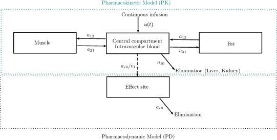
Figure 1: Schematic diagram of the PK/PD model with the effect site compartment of Bailey and Haddad Bailey .

2.1 Schnider’s Model

Following Schnider et al. Schnider , the lean body mass (LBM) is calculated using the James formula, which performs satisfactorily in normal and moderately obese patients, but not so well for severely obese cases James . The James formula calculates LBM as follows:

$$\text{for Male},\,\text{LBM} = 1.1\times\text{weight}-128\times\left(\dfrac{\text{weight}}{\text{height}}\right)^{2},$$ (3)

$$\text{for Female},\,\text{LBM} = 1.07\times\text{weight}-148\times\left(\dfrac{\text{weight}}{\text{height}}\right)^{2}.$$ (4)

The parameters of the PK/PD model (1) are then estimated according to Table 1.

Table 1: Parameter values for model (1) according to Schnider’s model Schnider .

Parameter	Estimation
$a_{10}\,(\text{min}^{-1})$	$0.443+0.0107\,(\text{weight}-77)-0.0159\,(\text{LBM}-59)+0.0062\,(\text{height}-177)$
$a_{12}\,(\text{min}^{-1})$	$0.302-0.0056\,(\text{age}-53)$
$a_{13}\,(\text{min}^{-1})$	0.196
$a_{21}\,(\text{min}^{-1})$	$\left(1.29-0.024\,(\text{age}-53)\right)/\left(18.9-0.391\,(\text{age}-53)\right)$
$a_{31}\,(\text{min}^{-1})$	0.0035
$a_{e0}\,(\text{min}^{-1})$	0.456
$v_{1}\,(\text{L})$	4.27

2.2 The Bispectral Index (BIS)

The BIS is the depth of anesthesia indicator, which is a signal derived from the EEG analysis and directly related to the effect site concentration of $x_{4}(t)$. It quantifies the level of consciousness of a patient from 0 (no cerebral activity) to 100 (fully awake patient), and can be described empirically by a decreasing sigmoid function Bailey :

$$BIS(x_{4}(t))=BIS_{0}\left(1-\dfrac{x_{4}(t)^{\gamma}}{x_{4}(t)^{\gamma}+EC_{50}^{\gamma}}\right),$$ (5)

where $BIS_{0}$ is the $BIS$ value of an awake patient typically set to 100, $EC_{50}$ corresponds to the drug concentration associated with $50\%$ of the maximum effect, and $\gamma$ is a parameter modeling the degree of nonlinearity. According to Haddad , typical values for these parameters are $EC_{50}$ = 3.4 mg/L and $\gamma=3$.

2.3 The Equilibrium Point

Following Zabi , the equilibrium point is obtained by equating the right-hand side of (1) to zero,

$$\left\{\begin{array}[]{l l}0=-(a_{1\,0}+a_{1\,2}+a_{1\,3})\,x_{1}+a_{2\,1}\,x_{2}+a_{3\,1}\,x_{3}+u,\\ 0=a_{1\,2}\,x_{1}-a_{2\,1}\,x_{2},\\ 0=a_{1\,3}\,x_{1}-a_{3\,1}\,x_{3},\\ 0=\frac{a_{e\,0}}{v_{1}}\,x_{1}-a_{e\,0}\,x_{4},\\ \end{array}\right.$$ (6)

with the condition

$$x_{4}=EC_{50}.$$ (7)

It results that the equilibrium point $x_{e}=\left(x_{e\,1},x_{e\,2},x_{e\,3},x_{e\,4}\right)$ is given by

$$x_{e\,1}=v_{1}\,EC_{50},\quad x_{e\,2}=\frac{a_{1\,2}\,v_{1}\,EC_{50}}{a_{2\,1}},\quad x_{e\,3}=\frac{a_{1\,3}\,v_{1}\,EC_{50}}{a_{3\,1}},\quad x_{e\,4}=EC_{50},$$ (8)

and the value of the continuous infusion rate for this equilibrium is

$$u_{e}=a_{1\,0}\,v_{1}\,EC_{50}.$$ (9)

The fast state is defined by

$$x_{eF}(t)=(x_{1}(t),x_{4}(t)).$$ (10)

The control of the fast dynamics is crucial because the BIS is a direct function of the concentration at the effect site.

3 Time-Optimal Control Problem

Let $x(t)=(x_{1}(t),x_{2}(t),x_{3}(t),x_{4}(t))\in\mathbb{R}^{4}$. We can write the dynamical system (1) in a matrix form as follows:

$$\dot{x}(t)=A\,x(t)+B\,u(t),$$ (11)

where

$$A=\left(\begin{array}[]{cccc}-(a_{1\,0}+a_{1\,2}+a_{1\,3})&a_{2\,1}&a_{3\,1}&0\\ a_{1\,2}&-a_{2\,1}&0&0\\ a_{1\,3}&0&-a_{3\,1}&0\\ \frac{a_{e\,0}}{v_{1}}&0&0&-a_{e\,0}\end{array}\right)\quad\text{ and }\quad B=\left(\begin{array}[]{c}1\\ 0\\ 0\\ 0\end{array}\right).$$ (12)

Here, the continuous infusion rate $u(t)$ is to be chosen so as to transfer the system (1) from the initial state (wake state) to the fast final state (anesthetized state) in the shortest possible time. Mathematically, we have the following time-optimal control problem Said :

$$\begin{cases}\min\limits_{t_{f}}J=\int\limits_{0}^{t_{f}}dt,\\ \dot{x}(t)=A\,x(t)+B\,u(t),\quad x(0)=(0,0,0,0),\\ C\,x_{eF}(t_{f})=x_{eF},\\ 0\leq u(t)\leq U_{max},\,\quad t\in[0,t_{f}],\,\quad t_{f}\,\text{is free,}\end{cases}$$ (13)

where $t_{f}$ is the first instant of time that the desired state is reached, and $C$ and $x_{eF}$ are given by

$$C=\left(\begin{array}[]{cc}1&0\\ 0&1\end{array}\right),\,\,\,\,x_{eF}=(x_{e1},\,x_{e4}),$$ (14)

with

$$x_{eF}(t_{f})=(x_{1}(t_{f}),x_{2}(t_{f})).$$ (15)

3.1 Pontryagin Minimum Principle

According to the Pontryagin minimum principle (PMP) Pontryagin , if $\tilde{u}\in L^{1}$ is optimal for Problem (13) and the final time $t_{f}$ is free, then there exists $\psi(t)=(\psi_{1}(t),\ldots,\psi_{4}(t))$, $t\in[0,t_{f}]$, $\psi\in AC([0,t_{f}];\mathbb{R}^{4})$, called the adjoint vector, such that

$$\begin{cases}\dot{x}=\displaystyle\frac{\partial H}{\partial\psi},\\[8.5359pt] \dot{\psi}=-\displaystyle\frac{\partial H}{\partial x},\end{cases}$$ (16)

where the Hamiltonian $H$ is defined by

$$H(t,x,u,\psi)=1+\psi^{T}\,(A\,x+B\,u).$$ (17)

Moreover, the minimality condition

$$H(t,\tilde{x}(t),\tilde{u}(t),\tilde{\psi}(t))=\min\limits_{0\leq u\leq U_{max}}H(t,\tilde{x}(t),u,\tilde{\psi}(t))$$ (18)

holds almost everywhere on $t\in[0,t_{f}]$.

Since the final time $t_{f}$ is free, according to the transversality condition of PMP, we obtain:

$$H(t_{f},x(t_{f}),u(t_{f}),\psi(t_{f}))=0.$$ (19)

Solving the minimality condition (18) on the interior of the set of admissible controls gives the necessary condition

$$\tilde{u}(t)=\begin{cases}0&\hbox{if}\,\,\tilde{\psi}_{1}(t)>0,\\ U_{max}&\hbox{if}\,\,\tilde{\psi}_{1}(t)<0,\end{cases}$$ (20)

where $\tilde{\psi}_{1}(t)$ is obtained from the adjoint system (16), that is, $\tilde{\psi}^{\prime}(t)=-A^{T}\tilde{\psi}(t)$, and the transversality condition (19). This is discussed in Sections 3.2 and 3.3.

3.2 Shooting Method

The shooting method is a numerical technique used to solve boundary value problems, specifically in the realm of differential equations and optimal control. It transforms the problem into an initial value problem by estimating the unknown boundary conditions. Through iterative adjustments to these estimates, the boundary conditions are gradually satisfied. In Bock , the authors propose an algorithm that addresses numerical solutions for parameterized optimal control problems. This algorithm incorporates multiple shooting and recursive quadratic programming, introducing a condensing algorithm for linearly constrained quadratic subproblems and high-rank update procedures. The algorithm’s implementation leads to significant improvements in convergence behavior, computing time, and storage requirements. For more on numerical approaches to solve optimal control problems, we refer the reader to Zaitri2019 and references therein.

Using (16), (17), (19), and (20), we consider the following problem:

$$\begin{cases}\dot{x}(t)=A\,x(t)+B\,\times\max\,(0,-U_{max}\,sign(\psi_{1}(t))),\\ \dot{\psi}(t)=-A^{T}\,\psi(t),\\ x(0)=(0,0,0,0),\,x_{1}(t_{f})=x_{e1},\,x_{4}(t_{f})=x_{e4},\\ \psi(0)\,\text{is free},\,H(t_{f},x(t_{f}),\max\,(0,-U_{max}\,sign(\psi_{1}(t_{f}))),\psi(t_{f}))=0.\end{cases}$$ (21)

Let $z(t)=(x(t),\psi(t))$. Then, we obtain the following two points’ boundary value problem:

$$\begin{cases}\dot{z}(t)=A^{*}z(t)+B^{*},\\ \textit{R}(z(0),z(t_{f}))=0,\end{cases}$$ (22)

where $A^{*}\in\textit{M}_{8\times 8}(\mathbb{R})$ is the matrix given by

$$A^{*}=\left(\begin{array}[]{cc}A&0_{4\times 4}\\ 0_{4\times 4}&-A^{T}\end{array}\right),$$ (23)

$B^{*}\in\mathbb{R}^{8}$ is the vector given by

$$B^{*}=\begin{cases}\left(0,\,0,\,0,\,0,\,0,\,0,\,0,\,0\right)&\hbox{if}\,\,\psi_{1}(t)>0,\\ \left(U_{max},\,0,\,0,\,0,\,0,\,0,\,0,\,0\right)&\hbox{if}\,\,\psi_{1}(t)<0,\end{cases}$$ (24)

and $R(z(0),z(t_{f}))$ is given by (2), (15), and (19). We consider the following Cauchy problem:

$$\begin{cases}\dot{z}(t)=A^{*}z(t)+B^{*},\\ z(0)=z_{0}.\end{cases}$$ (25)

If we define the shooting function $\textit{S}:\,\mathbb{R}^{4}\longrightarrow\mathbb{R}^{3}$ by

$$\textit{S}(z_{0})=\textit{R}(t_{f},z(t_{f},z_{0})),$$ (26)

where $z(t,z_{0})$ is the solution of the Cauchy problem (25), then the two points’ boundary value problem (21) is equivalent to

$$\textit{S}(z_{0})=0.$$ (27)

To solve (27), we use Newton’s method Newton .

3.3 Analytical Method

We now propose a different method to choose the optimal control. If the pair $(A,B)$ satisfies the Kalman condition and all eigenvalues of matrix $A\in n\times n$ are real, then any extremal control has at most $n-1$ commutations on $\mathbb{R}^{+}$ (at most $n-1$ switching times). We consider the following eight possible strategies:

Strategy 1 (zero switching times):

$$u(t)=U_{max},\,\forall t\in[0,t_{f}].$$ (28)

Strategy 2 (zero switching times):

$$u(t)=0,\,\forall t\in[0,t_{f}].$$ (29)

Strategy 3 (one switching time):

$$u(t)=\begin{cases}U_{max}&\hbox{if}\,\,0\leq t<t_{c},\\ 0&\hbox{if}\,\,t_{c}<t\leq t_{f},\end{cases}$$ (30)

where $t_{c}$ is a switching time.
Strategy 4 (one switching time):

$$u(t)=\begin{cases}0&\hbox{if}\,\,0\leq t<t_{c},\\ U_{max}&\hbox{if}\,\,t_{c}<t\leq t_{f}.\end{cases}$$ (31)

Strategy 5 (two switching times):

$$u(t)=\begin{cases}U_{max}&\hbox{if}\,\,0<t<t_{c1},\\ 0&\hbox{if}\,\,t_{c1}<t<t_{c2}.\\ U_{max}&\hbox{if}\,\,t_{c2}<t\leq t_{f},\\ \end{cases}$$ (32)

where $t_{c1}$ and $t_{c2}$ represent two switching times.
Strategy 6 (two switching times):

$$u(t)=\begin{cases}0&\hbox{if}\,\,0<t<t_{c1},\\ U_{max}&\hbox{if}\,\,t_{c1}<t<t_{c2}.\\ 0&\hbox{if}\,\,t_{c2}<t\leq t_{f}.\\ \end{cases}$$ (33)

Strategy 7 (three switching times):

$$u(t)=\begin{cases}U_{max}&\hbox{if}\,\,0<t<t_{c1},\\ 0&\hbox{if}\,\,t_{c1}<t<t_{c2}.\\ U_{max}&\hbox{if}\,\,t_{c2}<t\leq t_{c3}.\\ 0&\hbox{if}\,\,t_{c3}<t<t_{f},\\ \end{cases}$$ (34)

where $t_{c1}$, $t_{c2}$, and $t_{c3}$ represent three switching times.
Strategy 8 (three switching times):

$$u(t)=\begin{cases}0&\hbox{if}\,\,0<t<t_{c1},\\ U_{max}&\hbox{if}\,\,t_{c1}<t<t_{c2}.\\ 0&\hbox{if}\,\,t_{c2}<t\leq t_{c3}.\\ U_{max}&\hbox{if}\,\,t_{c3}<t<t_{f}.\\ \end{cases}$$ (35)

Let $x(t)$ be the trajectory associated with the control $u(t)$, given by the relation

$$x(t)=\exp(A\,t)\,x(0)+\int\limits_{0}^{t}\exp(A(t-s))Bu(t)ds,$$ (36)

where $\exp(A)$ is the exponential matrix of $A$.

To calculate the switching times $t_{c}$, $t_{c1}$, $t_{c2}$ and the final time $t_{f}$, we have to solve the following nonlinear equation:

$$\tilde{x}_{eF}(t_{f})=(x_{e1},\,x_{e4}).$$ (37)

We also solve (37) using the Newton method Newton .

4 Numerical Example

In this section, we use the shooting and analytical methods to calculate the minimum time $t_{f}$ to anesthetize a man of 53 years, $77$ kg, and $177$ cm.

The equilibrium point and the flow rate corresponding to a BIS of 50 are:

$$x_{e}=(14.518\,\text{mg},\,64.2371\,\text{mg},\,813.008\,\text{mg},\,3.4\,\text{mg}),\,\,\,u_{e}=6.0907\,\text{mg/min}.$$ (38)

Following the Schnider model, the matrix $A$ of the dynamic system (11) is given by:

$$A=\left(\begin{array}[]{cccc}-0.9175&0.0683&0.0035&0\\ 0.3020&-0.0683&0&0\\ 0.1960&0&-0.0035&0\\ 0.1068&0&0&-0.4560\end{array}\right)\quad\text{ and }\quad B=\left(\begin{array}[]{c}1\\ 0\\ 0\\ 0\end{array}\right).$$ (39)

We are interested to solve the following minimum-time control problem:

$$\begin{cases}\min\limits_{t_{f}}J=\int\limits_{0}^{t_{f}}dt,\\ \dot{x}(t)=A\,x(t)+B\,u(t),\quad x(0)=(0,\,0,\,0,\,0),\\ x_{e1}(t_{f})=14.518\,\text{mg},\quad x_{e4}(t_{f})=3.4\,\text{mg},\\ 0\leq u(t)\leq 106.0907,\quad t\in[0,t_{f}],\quad t_{f}\,\text{is free.}\end{cases}$$ (40)

4.1 Numerical Resolution by the Shooting Method

Let $z(t)=(x(t),\psi(t))$. We consider the following Cauchy problem:

$$\begin{cases}\dot{z}(t)=A^{*}z(t)+B^{*},\\ z(0)=z_{0}=(0,\,0,\,0,\,0,\,\psi_{01},\,\psi_{02},\,\psi_{03},\,\psi_{04}),\end{cases}$$ (41)

where

$$A^{*}=10^{-4}\left(\begin{array}[]{cccccccc}-9175&683&35&0&0&0&0&0\\ 3020&-683&0&0&0&0&0&0\\ 196&0&-35&0&0&0&0&0\\ 1068&0&0&-456&0&0&0&0\\ 0&0&0&0&9175&-3020&-196&-1068\\ 0&0&0&0&-683&683&0&0\\ 0&0&0&0&-35&0&35&0\\ 0&0&0&0&0&0&0&456\end{array}\right),\,$$ (42)

$$B^{*}=\left(\begin{array}[]{c}\max\,(0,-106.0907\,sign(\psi_{1}(t)))\\ 0\\ 0\\ 0\\ 0\\ 0\\ 0\\ 0\end{array}\right).$$ (43)

The shooting function S is given by

$$\textit{S}(z_{0})=(\textit{S}_{1}(z_{0}),\,\textit{S}_{2}(z_{0}),\,\textit{S}_{3}(z_{0})),$$ (44)

where

$$\textit{S}_{1}(z_{0}) = x_{e1}(t_{f})-14.518,$$

$$\textit{S}_{2}(z_{0}) = x_{e4}(t_{f})-3.4,$$

$$\textit{S}_{3}(z_{0}) = 1+\psi^{T}(t_{f})\left(Ax(t_{f})+B\max\,(0,-106.0907\,sing\,\psi_{1}(t_{f}))\right).$$

All computations were performed with the MATLAB numeric computing environment, version R2020b, using the medium-order method and the function ode45 (Runge–Kutta method) in order to solve the nonstiff differential system (22). We have used the variable order method and the function ode113 (Adams–Bashforth–Moulton method) in order to solve the nonstiff differential system (25), and the function fsolve in order to solve equation $\textit{S}(z_{0})=0$. Thus, we obtain that the minimum time is equal to

$$t_{f}=1.8397\,\text{min},$$ (45)

with

$$\psi^{T}(0)=(-0.0076,\,0.0031,\,-0.0393,\,-0.0374).$$ (46)

4.2 Numerical Resolution by the Analytical Method

The pair $(A,B)$ satisfies the Kalman condition, and the matrix $A$ has four real eigenvalues. Then, the extremal control $u(t)$ has at most three commutations on $\mathbb{R}^{+}$. Therefore, let us test the eight strategies provided in Section 3.3.

Note that the anesthesiologist begins with a bolus injection to transfer the patient state from the consciousness state $x(0)$ to the unconsciousness state

$$x_{eF}=(14.518,\,3.4),$$

that is,

$$u(0)=U_{max}=106.0907\,\text{mg/min}.$$ (47)

Thus, Strategies 2, 4, 6, and 8 are not feasible here. Therefore, in the sequel, we investigate Strategies 1, 3, 5, and 7 only.
Strategy 1: Let $u(t)=106.0907\,\text{mg/min}$ for all $t\in[0,t_{f}]$. The trajectory $x(t)$, associated with this control $u(t)$, is given by the following relation:

$$x(t)=\int\limits_{0}^{t}\exp(A(t-s))BU_{max}ds,\,\,\forall t\in[0,t_{f}],$$ (48)

where

$$\exp(A\,(t-s)) = V\,D(t-s)\,V^{-1}$$ (49)

with

$$V=\left(\begin{array}[]{cccc}0&0.9085&0.0720&-0.0058\\ 0&-0.3141&0.9377&-0.0266\\ 0&-0.1898&-0.3395&-0.9996\\ 1&-0.1997&0.0187&-0.0014\end{array}\right)$$ (50)

and

$$D(\tau)=\left(\begin{array}[]{cccc}\exp^{-0.4560\,\tau}&0&0&0\\ 0&\exp^{-0.9419\,\tau}&0&0\\ 0&0&\exp^{-0.0451\,\tau}&0\\ 0&0&0&\exp^{-0.0024\,\tau}\end{array}\right).$$ (51)

System (37) takes the form

$$\begin{cases}x_{1}(t_{f})=14.518,\\ x_{4}(t_{f})=3.4,\\ \end{cases}$$ (52)

and has no solutions. Thus, Strategy 1 is not feasible.
Strategy 3: Let $u(t),\,t\in[0,t_{f}],$ be the control defined by

$$u(t)=\begin{cases}106.0907\,\text{mg/min}&\hbox{if}\,\,0\leq t<t_{c},\\ 0&\hbox{if}\,\,t_{c}<t\leq t_{f}.\end{cases}$$ (53)

The trajectory $x(t)$ associated with this control $u(t)$ is given by

$$x(t)=\begin{cases}\int\limits_{0}^{t}\exp(A(t-s))BU_{max}ds&\hbox{if}\,\,0\leq t\leq t_{c},\\ \exp(A\,(t-t_{c}))\,x(t_{c})&\hbox{if}\,\,t_{c}<t\leq t_{f},\end{cases}$$ (54)

where

$$\exp(A\,(t-t_{c})) = V\,D(t-t_{c})\,V^{-1}.$$ (55)

To calculate the switching time $t_{c}$ and the final time $t_{f}$, we have to solve the nonlinear system (52) with the new condition

$$t_{c}<t_{f}.$$ (56)

Similarly to Section 4.1, all numerical computations were performed with MATLAB R2020b using the command solve to solve Equation (52). The obtained minimum time is equal to

$$t_{f}=1.8397\,\text{min},$$ (57)

with the switching time

$$t_{c}=0.5467\,\text{min}.$$ (58)

Strategy 5: Let $u(t)$, $t\in[0,t_{f}]$, be the control defined by the relation

$$u(t)=\begin{cases}106.0907\,\text{mg/min}&\hbox{if}\,\,0\leq t<t_{c1},\\ 0&\hbox{if}\,\,t_{c1}<t<t_{c2}.\\ 106.0907\,\text{mg/min}&\hbox{if}\,\,t_{c2}<t\leq t_{f},\\ \end{cases}$$ (59)

where $t_{c1}$ and $t_{c2}$ are the two switching times. The trajectory $x(t)$ associated with control (59) is given by

$$x(t)=\begin{cases}\int\limits_{0}^{t}\exp(A(t-s))BU_{max}ds&\hbox{if}\,\,0\leq t\leq t_{c1},\\ \exp(A\,(t-t_{c1}))\,x(t_{c1})&\hbox{if}\,\,t_{c1}<t\leq t_{c2},\\ \exp(A\,(t-t_{c2}))\,x(t_{c2})+\int\limits_{t_{c2}}^{t}\exp(A(t-s))BU_{max}ds&\hbox{if}\,\,t_{c2}<t\leq t_{f}.\end{cases}$$ (60)

To compute the two switching times $t_{c1}$ and $t_{c2}$ and the final time $t_{f}$, we have to solve the nonlinear system (52) with

$$0\leq t_{c1}\leq t_{c2}\leq t_{f}.$$ (61)

It turns out that System (52) subject to Condition (61) has no solution. Thus, Strategy 5 is also not feasible.
Strategy 7: Let $u(t)$, $t\in[0,t_{f}]$, be the control defined by the relation

$$u(t)=\begin{cases}106.0907\,\text{mg/min}&\hbox{if}\,\,0\leq t<t_{c1},\\ 0&\hbox{if}\,\,t_{c1}<t<t_{c2}.\\ 106.0907\,\text{mg/min}&\hbox{if}\,\,t_{c2}<t\leq t_{c3},\\ 0\,\text{mg/min}&\hbox{if}\,\,t_{c3}<t\leq t_{f},\\ \end{cases}$$ (62)

where $t_{c1}$, $t_{c2}$, and $t_{c3}$ are the three switching times. The trajectory $x(t)$ associated with Control (62) is given by

$$x(t)=\begin{cases}\int\limits_{0}^{t}\exp(A(t-s))BU_{max}ds&\hbox{if}\,\,0\leq t\leq t_{c1},\\ \exp(A\,(t-t_{c1}))\,x(t_{c1})&\hbox{if}\,\,t_{c1}<t\leq t_{c2},\\ \exp(A\,(t-t_{c2}))\,x(t_{c2})+\int\limits_{t_{c2}}^{t}\exp(A(t-s))BU_{max}ds&\hbox{if}\,\,t_{c2}<t\leq t_{c3},\\ \exp(A\,(t-t_{c3}))\,x(t_{c3})&\hbox{if}\,\,t_{c3}<t\leq t_{f}.\\ \end{cases}$$ (63)

To compute the three switching times $t_{c1}$, $t_{c2}$, and $t_{c3}$ and the final time $t_{f}$, we have to solve the nonlinear system (52) with

$$0\leq t_{c1}\leq t_{c2}\leq t_{c3}\leq t_{f}.$$ (64)

It turns out that System (52) subject to Condition (64) has no solution. Thus, Strategy 7 is also not feasible.

In Figures 2 and 3, we present the solutions of the linear system of differential equations (40) under the optimal control $u(t)$ illustrated in Figure 4, where the black curve corresponds to the one obtained by the shooting method, as explained in Section 3.2, while the blue curve corresponds to our analytical method, in the sense of Section 3.3. In addition, for both figures, we show the controlled BIS Index, the trajectory of fast states corresponding to the optimal continuous infusion rate of the anesthetic $u(t)$, and the minimum time $t_{f}$ required to transition System (40) from the initial (wake) state

$$x_{0}=(0,\,0,\,0,\,0)$$

to the fast final (anesthetized) state

$$x_{eF}=(14.518,\,3.4)$$

in the shortest possible time. The minimum time $t_{f}$ is equal to $t_{f}=1.8397\,\text{min}$ by the shooting method (black curve in Figure 2), and it is equal to $t_{f}=1.8397\,\text{min}$ by the analytical method (blue curve in Figure 3).

By using the shooting method, the black curve in Figure 4 shows that the optimal continuous infusion rate of the induction phase of anesthesia $u(t)$ is equal to $106.0907$ mg/min until the switching time

$$t_{c}=0.5467\,\text{min}.$$

Then, it is equal to $0\,\text{mg/min}$ (stop-infusion) until the final time

$$t_{f}=1.8397\,\text{min},$$

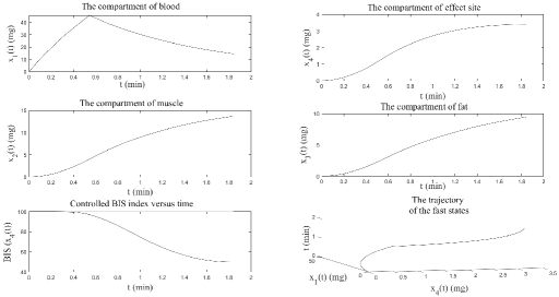
Figure 2: The state trajectory, controlled BIS index, and trajectory of the fast states corresponding to the optimal control $u(t)$ of Figure 4, using the shooting method.

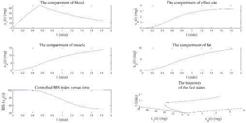
Figure 3: The state trajectory, controlled BIS index, and trajectory of the fast states corresponding to the optimal control $u(t)$ of Figure 4, using the analytical method.

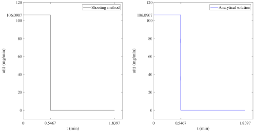
Figure 4: The optimal continuous infusion rate $u(t)$ of the induction phase of anesthesia, as obtained by the shooting and analytical methods.

By using the analytical method, the blue curve in Figure 4 shows that the optimal continuous infusion rate of the induction phase of anesthesia $u(t)$ is equal to $106.0907\,\text{mg/min}$ until the switching time

$$t_{c}=0.5467\,\text{min}.$$

Then, it is equal to $0\,\text{mg/min}$ (stop-infusion) until the final time

$$t_{f}=1.8397\,\text{min}.$$

We conclude that both methods work well and give similar results. However, in general, the shooting method does not always converge, depending on the initial conditions (46). To obtain such initial values is not an easy task since no theory is available to find them. For this reason, the proposed analytical method is logical, practical, and more suitable for real applications.

5 Conclusions

The approach proposed by the theory of optimal control is very effective. The shooting method was proposed by Zabi et al. Said , which is used to solve the time-optimal control problem and calculate the minimum time. However, this approach is based on Newton’s method. The convergence of Newton’s method depends on the initial conditions, being necessary to select an appropriate initial value so that the function is differentiable and the derivative does not vanish. This implies that the convergence of the shooting method is attached to the choice of the initial values. Therefore, the difficulty of the shooting method is to find the initial conditions of the adjoint vectors. Here, the aim was to propose a different approach, which we call “the analytical method”, that allows to solve the time-optimal control problem for the induction phase of anesthesia without such drawbacks. Our method is guided by the selection of the optimal strategy, without the need to choose initial values and study the convergence. We claim that our method can also be applied to other PK/PD models, in order to find the optimal time for the drug administration.

In the context of PK/PD modeling, the challenges associated with uncertainties in plant model parameters and controller gains for achieving robust stability and controller non-fragility are significant Elsisi . These challenges arise from factors like inter-individual variability, measurement errors, and the dynamic nature of patient characteristics and drug response. Further investigation is needed to understand and develop effective strategies to mitigate the impact of these uncertainties in anesthesia-related PK/PD models. This research can lead to the development of robust and non-fragile control techniques that enhance the stability and performance of anesthesia delivery systems. By addressing these challenges, we can improve the precision and safety of drug administration during anesthesia procedures, ultimately benefiting patient outcomes and healthcare practices. In this direction, the recent results of Mohamed may be useful. Moreover, we plan to investigate PK/PD fractional-order models, which is a subject under strong current research MR4539083 . This is under investigation and will be addressed elsewhere.

Conceptualization, M.A.Z., C.J.S., and D.F.M.T.; methodology, M.A.Z., C.J.S., and D.F.M.T.; software, M.A.Z.; validation, C.J.S. and D.F.M.T.; formal analysis, M.A.Z., C.J.S., and D.F.M.T.; investigation, M.A.Z., C.J.S., and D.F.M.T.; writing—original draft preparation, M.A.Z., C.J.S., and D.F.M.T.; writing—review and editing, M.A.Z., C.J.S. and D.F.M.T.; visualization, M.A.Z.; supervision, C.J.S. and D.F.M.T.; funding acquisition, M.A.Z., C.J.S., and D.F.M.T. All authors have read and agreed to the published version of the manuscript.

This research was funded by the Portuguese Foundation for Science and Technology (FCT—Fundação para a Ciência e a Tecnologia) through the R&D Unit CIDMA, Grant Numbers UIDB/04106/2020 and UIDP/04106/2020, and within the project “Mathematical Modelling of Multi-scale Control Systems: Applications to Human Diseases” (CoSysM3), Reference 2022.03091.PTDC, financially supported by national funds (OE) through FCT/MCTES.

Not applicable.

Not applicable.

No new data were created or analyzed in this study. Data sharing is not applicable to this article. The numerical simulations of Section 4 were implemented in MATLAB R2022a. The computer code is available from the authors upon request.

- (1) Evers, A.S.; Maze, M.; Kharasch, E.D. Anesthetic Pharmacology: Basic Principles and Clinical Practice, 2nd ed.; Cambridge University Press: Cambridge, UK, 2011.
- (2) Singh, N.; Sidawy, A.N.; Dezee, K.; Neville, R.F.; Weiswasser, J.; Arora, S.; Aidinian, G.; Abularrage, C.; Adams, E.; Khuri, S.; Henderson, W.G. The effects of the type of anesthesia on outcomes of lower extremity infrainguinal bypass. J. Vasc. Surg. 2006, 44, 964–970. https://doi.org/10.1016/j.jvs.2006.06.035.
- (3) Merry, A.F.; Mitchell, S.J. Complications of anaesthesia. Anaesthesia 2018, 73, 7–11. https://doi.org/10.1111/anae.14135.
- (4) Beck, C.L. Modeling and control of pharmacodynamics. Eur. J. Control 2015, 24, 33–49. https://doi.org/10.1016/j.ejcon.2015.04.006.
- (5) Meibohm, B.; Derendorf, H. Basic concepts of pharmacokinetic/pharmacodynamic (PK/PD) modelling. Int. J. Clin. Pharmacol. Ther. 1997, 35, 401–413.
- (6) Absalom, A.R.; Mani, V.; Smet, T.D.; Struys, M.M.R.F. Pharmacokinetic models for propofol—Defining and illuminating the devil in the detail. Br. J. Anaesth. 2009, 103, 26–37. https://doi.org/10.1093/bja/aep143.
- (7) Enlund, M. TCI : Target Controlled Infusion, or Totally Confused Infusion? Call for an Optimised Population Based Pharmacokinetic Model for Propofol. Upsala J. Med. Sci. 2008, 113, 161–170. https://doi.org/10.3109/2000-1967-222.
- (8) Oshin, T.A. Exploratory mathematical frameworks and design of control systems for the automation of propofol anesthesia. Int. J. Dyn. Control 2022, 10, 1858–1875. https://doi.org/10.1007/s40435-022-00953-1.
- (9) Wu, X.; Zhang, H.; Li, J. An analytical approach of one-compartmental pharmacokinetic models with sigmoidal Hill elimination. Bull. Math. Biol. 2022, 84, 117, 26. https://doi.org/10.1007/s11538-022-01078-4.
- (10) Nanditha, C.K.; Rajan, M.P. An adaptive pharmacokinetic optimal control approach in chemotherapy for heterogeneous tumor. J. Biol. Syst. 2022, 30, 529–551. https://doi.org/10.1142/S0218339022500188.
- (11) Wang, J.-J.; Dai, Z.; Zhang, W.; Shi, J.J. Operating room scheduling for non-operating room anesthesia with emergency uncertainty. Ann. Oper. Res. 2023, 321, 565–588. https://doi.org/10.1007/s10479-022-04870-6.
- (12) Schnider, T.W.; Minto, C.F.; Gambus, P.L.; Andresen, C.; Goodale, D.B.; Shafer, S.L.; Youngs, E.J. The influence of method of administration and covariates on the pharmacokinetics of propofol in adult volunteers. Anesthesiology 1998, 88, 1170–1182. https://doi.org/10.1097/00000542-199805000-00006.
- (13) Marsh, B.; White, M.; Morton, N.; Kenny, G.N. Pharmacokinetic model driven infusion of propofol in children. Br. J. Anaesth. 1991, 67, 41–48. https://doi.org/10.1093/bja/67.1.41.
- (14) Zabi, S.; Queinnec, I.; Tarbouriech, S.; Garcia, G.; Mazerolles, M. New approach for the control of anesthesia based on dynamics decoupling. IFAC-PapersOnLine 2015, 48, 511–516. https://doi.org/10.1016/j.ifacol.2015.10.192.
- (15) Zabi, S.; Queinnec, I.; Garcia, G.; Mazerolles, M. Time-optimal control for the induction phase of anesthesia. IFAC-PapersOnLine 2017, 50, 12197–12202. https://doi.org/10.1016/j.ifacol.2017.08.2279.
- (16) Ilyas, M.; Khan, A.; Khan, M.A.; Xie, W.; Riaz, R.A.; Khan, Y. Observer design estimating the propofol concentration in PKPD model with feedback control of anesthesia administration. Arch. Control Sci. 2022, 32, 85–103. https://doi.org/10.24425/acs.2022.140866.
- (17) Bock, H.G.; Plitt, K.J. A Multiple shooting algorithm for direct solution of optimal control problems. IFAC Proc. Vol. 1984, 17, 1603–1608. https://doi.org/10.1016/S1474-6670(17)61205-9.
- (18) Pontryagin, L.S.; Boltyanskii, V.G.; Gamkrelidze, R.V.; Mishchenko, E.F. The Mathematical Theory of Optimal Processes; Trirogoff, K.N., Ed.; Neustadt, L.W., Ed.; Interscience Publishers John Wiley and Sons, Inc.: New York, NY, USA, 1962.
- (19) Bailey, J.M.; Haddad, W.M. Drug dosing control in clinical pharmacology. IEEE Control Syst. Mag. 2005, 25, 35–51. https://doi.org/10.1109/MCS.2005.1411383.
- (20) James, W.P.T. Research on obesity: A report of the DHSS/MRC Group. Nutr. Bull. 1977, 4, 187–190. https://doi.org/10.1111/j.1467-3010.1977.tb00966.x.
- (21) Haddad, W.M.; Chellaboina, V.; Hui, Q. Nonnegative and Compartmental Dynamical Systems; Princeton Univ. Press: Princeton, NJ, USA, 2010.
- (22) Zaitri, M.A.; Bibi, M.O.; Bentobache, M. A hybrid direction algorithm for solving optimal control problems. Cogent Math. Stat. 2019, 6, 1612614. https://doi.org/10.1080/25742558.2019.1612614.
- (23) Deuflhard, P. Newton Methods for Nonlinear Problems; Springer Series in Computational Mathematics; Springer: Berlin, Germany, 2004; Volume 35.
- (24) Elsisi, M.; Soliman, M. Optimal design of robust resilient automatic voltage regulators. ISA Trans. 2021, 108, 257–268. https://doi.org/10.1016/j.isatra.2020.09.003.
- (25) Mohamed, M.A.E.; Mohamed, S.M.R.; Saied, E.M.M.; Elsisi, M.; Su, C.-L.; Hadi, H.A. Optimal energy management solutions using artificial intelligence techniques for photovoltaic empowered water desalination plants under cost function uncertainties. IEEE Access 2022, 10, 93646–93658. https://doi.org/10.1109/ACCESS.2022.3203692.
- (26) Morales-Delgado, V.F.; Taneco-Hernández, M.A.; Vargas-De-León, C.; Gómez-Aguilar, J.F. Exact solutions to fractional pharmacokinetic models using multivariate Mittag-Leffler functions. Chaos Solitons Fractals 2023, 168, 113164. https://doi.org/10.1016/j.chaos.2023.113164.