Simulation-driven engineering for the management of harmful algal and cyanobacterial blooms

Abstract

Harmful Algal and Cyanobacterial Blooms (HABs), occurring in inland and maritime waters, pose threats to natural environments by producing toxins that affect human and animal health. In the past, HABs have been assessed mainly by the manual collection and subsequent analysis of water samples and occasionally by automatic instruments that acquire information from fixed locations. These procedures do not provide data with the desirable spatial and temporal resolution to anticipate the formation of HABs. Hence, new tools and technologies are needed to efficiently detect, characterize and respond to HABs that threaten water quality. It is essential nowadays when the world’s water supply is under tremendous pressure because of climate change, overexploitation, and pollution. This paper introduces DEVS-BLOOM, a novel framework for real-time monitoring and management of HABs. Its purpose is to support high-performance hazard detection with Model Based Systems Engineering (MBSE) and Cyber-Physical Systems (CPS) infrastructure for dynamic environments.

1 Introduction

Harmful Algal and Cyanobacterial Blooms (HABs) constitute an especially relevant public health hazard and ecological risk, due to their frequent production of toxic secondary metabolites. Exposure to cyanotoxins, for instance, can cause severe health effects in humans and animals, as well as significant economic losses in local communities.

HABs typically emerge in a variety of freshwater ecosystems like reservoirs, lakes, and rivers Vincent2009 . Their intensity and frequency have increased globally during the last decade, mainly due to the current vulnerability of water resources to environmental changes, such as global warming, population growth, and eutrophication. For example, in 2014, a Microcystis HAB at the water treatment plant intake for Toledo (Ohio, USA) caused the distribution of non-potable water for more than 400000 people during multiple days Schmale2019 . The danger is not limited to the closest water environment since extracellular material from freshwater HABs has been observed in the water and the atmosphere at locations far beyond their edges.

During the last 30 years, the data needed to estimate the health of a water body and the possible existence of HABs have been obtained by specialized personnel through manual collection of water samples and subsequent analysis in the laboratory, and, in the best cases, by automatic instruments placed at fixed locations, that acquire data and, in very few cases, samples. Financial and personnel resource restrictions reduce the manual collection to the moments of the year when HABs are more likely to appear at a few geographical points and with minimal frequencies. The delay suffered by analytical results and the limited capacity to interpret the current scenario reduces the reaction (prediction, prevention, and mitigation) capability of the authorities responsible for the distribution of drinking water and its recreational uses Meriluoto2017 . This is critical when deploying Early-Warning Systems (EWSs), whose essential work is to collect water samples and identify the cyanobacterial cell or algae density as soon as possible. Hence, it is crucial to develop new cost-effective monitoring and early detection systems capable of predicting and anticipating when and where HABs form and produce toxins to provide support to water managers/authorities for guiding their policies and protecting the public health through the deployment of effective EWSs.

In this context, Modeling and Simulation (M&S) can be used to clarify the dynamics of HABs, as it has historically done in similar areasUng1972 . Numerical-based and data-driven machine learning models have been extensively used to simulate HABs in aquatic systems Long2011 ; Pyo2019 . These techniques try to reach accurate predictions through what we call base models. These models have been integrated into more generic software tools like the EE Modeling System (EEMS) EEMS2022 . Based on these models and tools, various countries have attempted to build EWSs with the support of predictive systems Wu2022 .

Our vision is, however, oriented to a system of systems architecture, a more holistic and integrative model that includes not only the use of the aforementioned base models but also the infrastructure of the EWS. Figure 1 shows our conception of the simulation framework, tightly coupled to the represented Cyber-Physical Systems (CPS). As Figure 1 illustrates, our framework follows a Internet of Things (IoT)-based architecture through the use of Digital Twins (DTs). Water bodies are monitored in the edge layer by a set of sensors, including those onboard automated boats, called here-after Unmanned Surface Vehicles (USVs), that continuously send data to the server at the nearest Ground Control Station (GCS) in the fog layer. There, domain experts can analyze the data, run some models, tests, or plan the USVs trajectories. The framework supports horizontal scalability, being able to add more water bodies with the support of a cloud layer, where authorities can compare different reports and make high-level decisions.

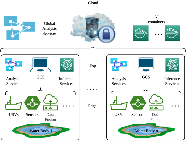
Figure 1: Conceptual model of the proposed framework.

To simulate and operate this complex model, in this paper we propose DEVS-BLOOM, a novel M&S framework to enable real-time monitoring and hazard prediction of HABs. Our approach is based on the principles of Model Based Systems Engineering (MBSE): (i) model-based since MBSE is based on the use of models to represent and manage information about a system, (ii) system-centric, focusing on the system as a whole, (iii) iterative and incremental process, which involves the development of models over time, (iv) collaboration between stakeholders, including system engineers, domain experts, etc., (v) traceability between requirements, design, and implementation, (vi) reuse of models, components, and other artifacts to improve efficiency and reduce the risk of errors, and (vii) verification and validation to ensure that the system meets its requirements and that it operates as intended Wymore2018 . At the same time, we aim to provide high-performance real-time services, such as detecting outliers or executing complex forecasting methods. All this is achieved through the implementation of model-driven technologies and infrastructure based on the IoT and DTs paradigms. As a result, we address three main topics in the sustainable management of water resources under the umbrella of model-driven technologies: (i) provide a robust interface to design intelligent HABs management system prototypes, (ii) provide vertical scalability, modeling the whole pyramidal structure, from the sensors to the authorities, and (iii) provide horizontal scalability, being able of adding more sensors and water bodies with the support of well-grounded M&S methodologies.

The main contributions of this work can be summarized as follows:

• We present a framework where we can model the water body, the infrastructure needed to monitor and manage HABs like sensors or USVs, the computing resources needed to control that infrastructure like workstations or cloud servers, and the actions performed by the human team like operators, domain experts, or water authorities.

• The model can be simulated in virtual mode to analyze the viability of the whole system; in hybrid mode, where some components are virtual, and others like actual sensors are co-simulated to test or calibrate these sensors; or in real mode, where the framework is not a simulator but a fully operational toolkit, where all the components are real.

• The framework supports horizontal scalability, allowing us to incorporate more water bodies, or vertical scalability, allowing us to elaborate more complex models. This is possible with the parallel or distributed execution of the framework, which the internal libraries automatically provide.

DEVS-BLOOM has been developed through the Discrete Event System Specification (DEVS) Zeigler2018 , a well known M&S formalism. To prove the feasibility of each scenario, the framework uses formal models. It can be fed with authentic or synthetic data. Following the MBSE methodology, DEVS-BLOOM has been designed with the main objective that any virtual component is built as a DT and can be replaced by its real-world counterpart Marcosig2018 .

The paper is organized as follows. In the following, we introduce the related work, focused on EWSs, models of HABs behavior, USVs trajectory planning, IoT simulators and all the elements required by the proposed framework. Next, we present the architecture of our framework based on a well-known M&S formalism. Then we illustrate the simulations performed to test our hypotheses and show the results obtained under different initial conditions. Finally, we draw some conclusions and introduce future lines of research.

2 Related work

As stated above, HABs pose severe threats to natural environments. To properly detect, assess, and mitigate these threats in inland waters, it is essential to envision water management from the perspective of an integrative IoT-based early warning system. HAB-centric automated EWSs can effectively help to monitor and treat water bodies since, once deployed, mitigation techniques tailored to those systems can be better designed.

Current EWSs are supported by a comprehensive set of accurate base models that describe the behavior of different elements, such as the dynamics of the water (due to currents and wind) and of the cyanobacteria (due to biological growth, their vertical displacements, and the water dynamics). There exist a significant variability of base models. Eulerian models, for instance, have been used since 1970 to simulate eutrophication, water quality, and biogeochemical processes Vinccon2019 . These models are composed of differential equations that simulate community dynamics in spaces. Lagrangian models introduce the possibility of adding different classes of particles with individualized properties, although conducting Lagrangian simulations with a large number of particles is a computer-intensive process VanSebille2018 . Machine learning techniques can also be used to clarify the dynamics of HABs. Based on studies from 2008 to 2019, Chen et al. show in Chen2020 numerous applications of machine learning models for predicting various water quality variables, such as salinity, pH, electrical conductivity, dissolved oxygen, ammonium nitrogen, etc. Finally, we may also find mechanistic or process-oriented aquatic models based on knowledge of how target species respond to various ecosystem drivers like nutrient availability, thermal stratification, life cycle characteristics of species, etc. Rousso2020 . These models can be more appropriate than statistically based models for future predictions. However, they can be challenging because the incomplete knowledge introduced inside the models forces the incorporation of complex Bayesian networks, adding even more uncertainty to the models.

The previous base models are usually integrated inside more generic software tools with advanced Graphical User Interfaces (GUIs). For instance, EEMS EEMS2022 is a GUI that provides a broad range of pre-processing and post-processing tools to assist in developing, calibrating, and analyzing hydrodynamic, sediment-contaminant, and eutrophication models. MIKE Powered by DHI is a range of software products that enable us to accurately analyze, model and simulate any type of challenge in water environments MIKE2022 . Delft3D is a set of open source software tools that facilitates modeling subsystems like the hydrodynamic, morphodynamic, waves, water quality, or particle-based subsystems Delft2022 .

Finally, the aforementioned base models along with the GUIs are used in EWSs as forecasting tools Velez2014 ; Silva2016 , helping GCS operators to make critical decisions. An example close to the authors of this paper is the Spanish Automatic Water Quality Information System, which is a network of nearly 200 automatic alert stations deployed in critical locations of the Spanish hydrographic system to (i) obtain frequent measurements of representative parameters such as water temperature, pH and dissolved oxygen; (ii) provide valuable information about the general quality of the water; and (iii) alert in real time about pollution episodes Serramia2004 . More examples of EWSs can be found in other places and settings. The Southeast Environmental Research Center Water Quality Monitoring Network, property of Florida International University, focuses on coastal monitoring of the southern tip of the Florida peninsula and includes some automatic measuring stations that are rotated between the different sampling sites SERC2022 . United States Geological Survey’s National Water Quality Monitoring Network combines data sources and techniques from 110 sites to monitor the U.S. inland waters Riskin2021 . Environment and Climate Change Canada, in collaboration with the provincial and territorial governments, runs the Freshwater Quality Monitoring and Surveillance program, which encompasses some manual and automatic monitoring networks distributed through the national territory FWQMS2022 .

The conception, design, and deployment of an EWS can present complex engineering and systems challenges. To properly monitor and foresee the formation of HABs, EWSs must cover large geographical areas, remain functional over long periods, and include a large variety of sensors, USVs, and data in general. Prediction of HABs also involves the use of a plethora of base models. A model-driven approach to designing such a complex and heterogeneous infrastructure would help researchers, domain experts, and water authorities to meet design requirements. It also would enable a model-driven control, reducing costs while increasing performance and scalability, and in general, all the benefits derived from applying a MBSE approach. There exist cases of success in other areas of research like flood detection Basha2008 , water treatment Curl2019 , or healthcare Henares2022 . However, to our knowledge, this is the first research related to developing integrative model-driven solutions for HAB management. As mentioned above, our approach is integrative because we do not simulate only the water body but also combine the use of base models with the help of models of the infrastructure like sensors, USVs, GCSs, the cloud layer, and even the operator’s behavior through a simulation file, which is the main novelty with respect to other approaches in the literature.

3 System architecture and design

DEVS-BLOOM’s model divides the HAB management system into the three classical IoT layers: edge, fog, and cloud. The edge layer includes all the devices connected to the internet and can generate data. These devices can be sensors, wearables, and other smart devices deployed in the field. The edge layer collects and processes data locally and then sends it to the next layer for further processing. The fog layer is an intermediate layer between the edge and the cloud. This layer includes devices with computing power and storage capabilities to perform basic data processing and analysis. The fog layer is responsible for processing data in real time and reducing the amount of data that needs to be sent to the cloud for further processing. The cloud layer includes cloud servers and data centers that can store and process large amounts of data. The cloud layer performs complex data analytics and machine learning tasks that require significant computing power and storage capacity J-Cardenas2021 .

Figure 1 has already illustrated the general picture of the framework architecture. Our M&S framework is fed with data that may come from the actual water body or from a database, which can, in turn, store authentic or synthetic data. The virtual/real duality developed into some components, modeled as DTs, allows DEVS-BLOOM to work in virtual, real, or hybrid modes. The framework works in virtual/simulation mode when data come entirely from the database. Real/controller mode is when data come from the real water body, with actual sensors and USV deployed and the system fed with real data. Currently, DEVS-BLOOM is mostly used for infrastructure analysis and design. Thus, data usually come from the database; therefore, DEVS-BLOOM works in virtual/simulation mode. However, sometimes a prototype sensor or USV is tested for validation on the field, and then DEVS-BLOOM works in hybrid mode, where some virtual components are simulated and the actual ones are being controlled.

To clarify the specifics of the DEVS nomenclature, we first describe the basic principles of the formalism. Next, the DEVS-BLOOM system architecture is explained.

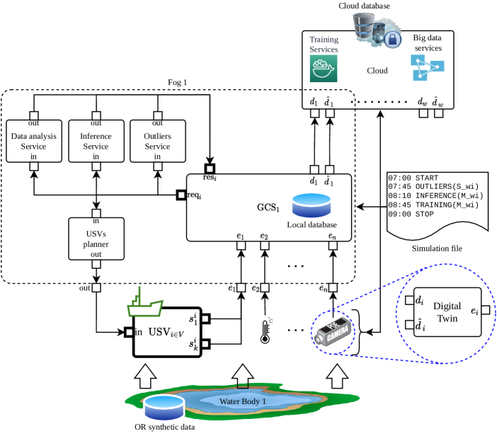
Figure 2: DEVS root coupled model of the system architecture.

3.1 The DEVS formalism

Parallel DEVS is a modular and hierarchical formalism for modeling discrete event systems based on set theory Zeigler2018 . It includes two types of models, atomic and coupled, that have an interface consisting of input ($X$) and output ($Y$) ports to communicate with other models. Additionally, in atomic models, every model state ($S$) is associated with the time advance function $ta$, which determines the duration in which the state remains unchanged.

Once the time assigned to the state has passed, an internal transition is triggered and the corresponding function ($\delta_{\rm int}:S\rightarrow S$) is invoked, producing a local state change ($\delta_{\rm int}(s)=s^{\prime}$). At that time, the results of the model execution are spread through the output ports of the model by activating an output function ($\lambda$).

Furthermore, external input events (received from other models) are collected in the input ports. An external transition function ($\delta_{\rm ext}:S\times e\times X\rightarrow S$) specifies how to react to those inputs, using the current state ($s$), the elapsed time since the last event ($e$) and the input value ($x$) ($\delta_{\rm ext}((s,e),x)=s^{\prime}$). Parallel DEVS introduces a confluent function ($\delta_{\rm con}((s,ta(s)),x)=s^{\prime}$), which decides the next state in cases of collision between external and internal transitions.

Coupled models are the aggregation/composition of two or more models (atomic and/or coupled), connected by explicit couplings. This makes DEVS closed under coupling and allows us to use networks of systems as components in larger coupled models, leading to hierarchical and modular designs.

Overall, DEVS provides a framework for information modeling that has several advantages in the analysis and design of complex systems: completeness, verifiability, extensibility, and maintainability.

Once a system is described according to DEVS theory, it can be easily implemented using one of the many DEVS M&S engines available J-RiscoMartin2022b .

DEVS-BLOOM is implemented and executed using xDEVS, a cross-platform DEVS simulator. This library includes a set of C, C++, C#, Go, Java, Python, and Rust repositories that provide equivalent DEVS interfaces. The project’s final goal is to elaborate the fastest DEVS simulation interface with the capacity to simulate models in virtual and real-time and to run simulations in sequential (single-threaded), parallel (multi-threaded), and distributed (not shared memory) architectures. In particular, DEVS-BLOOM uses the xDEVS/Python module of the project. As in xDEVS, our framework can use virtual or real-time. It can run sequential or parallel simulations without modifying a single line of code in the underlying simulation model.

3.2 DEVS-BLOOM

The DEVS-BLOOM root coupled model is depicted in Figure 2. The components included in this coupled model are: sensors and USVs at the edge layer, the fog coupled model, and the cloud atomic model.

There exist one singular atomic model labeled as Simulation file in Figure 2. It is just a source that reads from a text file all the events that will be injected into the simulation process through its output port. Output and explicit connections related to this atomic model are not explicitly represented in Figure 2 for simplicity because this atomic model is connected to all the components of DEVS-BLOOM. Each entry in the simulation file represents an input event composed of: a time mark indicating the virtual instant in which this event will be triggered, the command type associated with the event, and the arguments each command needs. As a result, this file replicates the set of external events that could happen in a real-world scenario. As the excerpt of Figure 2 illustrates, it always begins and ends with the triggering of the initialization and finalization of the simulation experiment (see START and STOP commands). Some services can be triggered in the middle, like outliers detection or HAB prediction. The simulation file is a pure virtual element, which does not have an exact match in the real world. In the following sections, we describe the rest of the components included in DEVS-BLOOM.

3.2.1 Edge layer

The atomic models in this layer represent edge devices such as environmental sensors, cameras placed at stationary positions, and USVs. Particularly, sensors are implemented as DTs and can process data from the actual sensor or the database mentioned above. A representation of an atomic sensor model is illustrated in Figure 2, labeled as Digital Twin. Data from its real counterpart is received through the $d_{i}$ input port. In this case, data is just propagated without extra delays to the corresponding output port $e_{i}$. On the other hand, data from the database is received by the $\hat{d}_{i}$ input port. Here the virtual sensor imitates the behavior of the actual sensor, introducing corresponding delays, noise, saturation errors, aging, etc. All these optional parameters are defined through a configuration file. Like most DEVS-BLOOM components, this is a passive atomic model, which is awakened when it receives a START event from the simulation file.

Each DT transmits, at their discretion, events that follow a predefined and generic structure that encapsulates the measurements, commands, or any other relevant information. That generic event structure, represented in Figure 3, carries a timestamp with the actual event time, a source and id that respectively identify the source and the cause of the event, and a payload which contains a set of key-value pairs with the actual measurements (e.g. ’Lat’: 47.0, ’Lon’: -122.0, ’Depth’:-0.2, ’TEM’: 19.0). Finally, any time an event is generated, it is transmitted through the corresponding output port $e_{i}$, which in this case is connected to the fog coupled model of the water body, where the data will be curated and stored in the local fog database.

⬇

id:’DOX’,

source: ’SimSenO’,

timestamp:’2021-08-23 00:30:05’,

payload:

{’Lat’:47.50502,’Lon’:-122.21501,

’Depth’:0.00,’DOX’:8.69}

⬇

...

DOX,SimSenO,2008-08-23 00:00:00,{’id’:’DOX’,’description’:’Oxigen Sensor(mg/L)’,’delay’:5,
’max’:30.0,’min’:0.0,’precision’:0.1,’noisesigma’:0.2}

...

DOX,SimSenO,2008-08-23 01:30:05,{’Lat’:47.5050,’Lon’:-122.2150,’Depth’:0.0,’DOX’:11.8}

NOX,SimSenN,2008-08-23 01:30:06,{’Lat’:47.5050,’Lon’:-122.2150,’Depth’:0.0,’NOX’:0.152}

TEM,SimSenT,2008-08-23 01:30:07,{’Lat’:47.5050,’Lon’:-122.2150,’Depth’:0.0 ,’TEM’:19.6}

...

IRA,VirSenI,2008-08-23 08:30:02, {’Lat’:47.5000,’Lon’:-122.2200,’IRA’: 0.60}

...

Figure 3: Generic event structure. On the left, the serialization of a typical event object generated at the edge layer. On the right, an excerpt of messages stored at the local database of fog layer.

DEVS-BLOOM can handle a set $\mathbf{V}$ of USVs atomic models, illustrated as a box with bold lines and ports in Figure 2. USVs receive communications from the fog coupled model or other USVs since they are also interconnected to avoid collisions or to share information. Each USV has $K$ output ports ($s^{i\in V}_{k\in K}$) to transmit the information gathered by USV sensors related to aquatic variables (e.g. temperature, pH, and chlorophyll-a and phycocyanin fluorescence) and to the USV state (e.g. power, position).

3.2.2 Fog layer

The fog layer is modeled through the fog coupled model, which mainly represents the GCS associated with the water body. Here, operators and domain experts analyze data, make decisions, and take action. It is worthwhile to mention that DEVS-BLOOM can predict the bloom appearance, automatically guide USVs to the zone of interest, or take measurements. Still, all these actions must be validated or complemented by the operators. There can be as many fog-coupled models as water bodies being analyzed by the same cloud infrastructure. Figure 2 represents the first of them. As the Figure shows, the fog coupled model has several input ports that receive the events sent by the DTs located at the edge layer (sensors and USVs). It also has two output ports that send raw data collected by the sensors to the cloud and augmented or fixed sensor data using outliers detection or data analysis services, through $d_{1}$ and $\hat{d}_{1}$ ports, respectively. To reduce visual clutter, Figure 2 does not explicitly represent the coupling relations between fog and cloud. It is quite redundant and makes the Figure unnecessarily large. Basically, $d_{1}$ and $\hat{d}_{1}$ are connected through two additional external output couplings (from GCS₁ to Fog₁) and two internal couplings (from Fog₁ to Cloud). The fog coupled model contains several atomic models, detailed below.

The GCS atomic model represents the core of the computing infrastructure of the control station. It is usually a static workstation or laptop connected to the local network. This simplified DT receives simulation commands from the simulation file atomic model, which tell the computer when to start reading data, execute an outliers detection service, an inference over the HAB predictive models, USVs path planning, etc. When the simulation starts, sensor data are received through the $e_{i}$ input ports and stored in the local database. These data are sent through the $d_{1}$ fog output port, which is connected to the $d_{1}$ cloud input port. On the other hand, when a service request is received from the simulation file, it is propagated through the output port $req_{i}$, which is connected to the corresponding atomic model. This port is drawn in bold in Figure 2 because it represents a set of output ports. Fixed or predicted data are also stored in the local database and regularly sent through the $\hat{d}_{1}$ output port, connected to the $\hat{d}_{1}$ cloud input port.

The fog coupled model also has a set of atomic models in charge of executing services. They are currently part of the GCS ₁ atomic model in the real system. Still, we have decided to implement them as external atomic models to separate the services, models, or functions that they incorporate. These atomic models receive commands from the in input port and send the results through the out output ports. These output ports are connected back to the GCS or the USV atomic models, controlling the navigation system of the USVs. We have currently deployed four services: one to detect and fix outliers, labeled as Outliers services in Figure 2, another one to perform inference and compute the probability of HAB formation and location in the water body, labeled as Inference service, a third one to carry out data analysis over the database and generate reports, named Data analysis service, and the last one is the USVs path planner, as labeled in Figure 2, which taking the probabilities computed by the inference service calculates and sends the waypoints and trajectories that USVs must follow.

3.2.3 Cloud layer

Finally, the cloud atomic model is located in the cloud layer. It receives all the data from different water bodies (raw and estimated, i.e., fixed or predicted) and stores them in the central cloud database. As in the fog coupled model, the cloud atomic model can run different services but is highly scaled to handle one or several water bodies. These services include executing big data analyses involving all the data stored in the central database or running training services to update current inference models located at the fog-coupled models. In any case, these actions are always triggered by the simulation file. We have not included dedicated atomic models to run services because they are always processes installed in docker containers, i.e., they have a distributed architecture. They do not need to be encapsulated as DEVS models, i.e., the cloud layer is viewed as a centralized entity.

DEVS-BLOOM scalability is ensured since our framework has been designed to consider possible scalability issues, allowing users to externalize and scale critical services in case of a bottleneck. For instance, DEVS atomic models that consume more resources, like those designed to run training or data analysis services, can be easily simulated in parallel or distributed computing architectures J-RiscoMartin2022 .

4 Use cases

This Section presents two simulation scenarios to test the developed framework. Additionally, this Section illustrates how an actual sensor in DEVS-BLOOM can replace a virtual one and show some advances in the design of the real USV, which is evolving with the corresponding DEVS-BLOOM USV model.

Figure 4 shows the DEVS-BLOOM model used in this Section. It is a particular case of the general model depicted in Figure 2, used to monitor a water body corresponding to an area of Lake Washington.

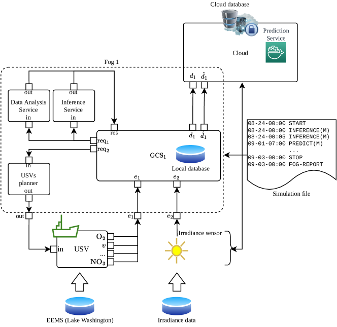
Figure 4: DEVS-BLOOM root coupled model of the use case.

We provide more details of each atomic model instance included in Figure 4 throughout each use case.

4.1 Monitoring use case

The monitoring scenario is relevant for operators and domain experts in charge of the GCS and local operative decisions, monitoring HABs state and evolution through the use of a USV, i.e., it shows how DEVS-BLOOMS is used to predict the next location of the HAB and to automatically control the USV to follow the position and confirm the prediction.

In this case, the whole water body dataset is synthetic and generated with the EEMS tool EEMS2022 , which incorporates an accurate model of Lake Washington. It allows us the artificial generation of HABs. As a result, DEVS-BLOOM receives EEMS input data (see Figure 4) that includes water speed, water temperature, oxygen and nitrates densities, and for validation of our framework, algae concentration.

Additionally, as Figure 4 shows, we have included a virtual irradiance sensor, which generates synthetic irradiance data taken from PVGIS. Neither EEMS nor PVGIS give stochastic data, so there is no need to proceed with Monte Carlo simulations.

Our scenario has at the edge layer a USV that must monitor the water and transmit data to the fog and cloud layers. As Figure 4 depicts, the USV is instrumented with several sensors and units. Some of them take data from the water body to continuously monitor the state of the bloom and feed the inference model, and others from internal component models:

• Temperature sensor: is in charge of measuring the water temperature. This signal influences the calibration of other sensors and the growth dynamics of the bloom.

• Power unit: includes solar panels, chargers, and batteries in charge of recharging the boat’s batteries when it receives solar radiation. For this scenario, we have included the following base model:

  $$prop = K_{p}\cdot\sqrt{e_{lat}^{2}+e_{lon}^{2}}$$

  $$power = K_{e}+K_{s}\cdot sun-prop$$

  $K_{p}=30$ is the propulsion constant, $K_{e}=-0.003$ represent the electronic power consumption, $K_{s}=0.04$ is the sun power factor, $prop$ is the resultant propulsion, $e_{lat}$ and $e_{lon}$ are the latitude and longitude error of the USV with respect to the HAB position, computed by the USV planner atomic model, $power$ is the battery energy level, and $sun$ is the normalized irradiance value.

• Flow meter: measures the speed and direction of the water with respect to the ship. We may infer the water’s speed and direction by discounting the ship’s speed.

• Positioning unit: allows us to measure the position and speed of the ship, following these two equations:

  $$lat_{usv} = e_{lat}+K_{2d}\cdot wfv$$

  $$lon_{usv} = e_{lon}+K_{2d}\cdot wfu$$

  $K_{2d}=0.01$ is the 2D USV displacement constant, and $(wfv,wfu)$ is the water speed (north and east components).

• Dissolved oxygen probe: is in charge of measuring the dissolved oxygen density in the water. If there are high levels of oxygen, there may be a bloom of algae that produces oxygen by photosynthesis.

• Nitrogen probe: measures the density of dissolved nitrates in the water. Nitrate is the main food for algae. Therefore, the inference service uses this signal to predict the bloom’s growth.

During the simulation, irradiance and USV sensors capture measurements and send them to the fog layer. We utilize the inference service in this layer, shown in Figure 4. It has a predictive model based on differential equations that, using water speed, temperature, coordinates, oxygen and nitrates densities, and solar irradiance, anticipates the emergence and displacement of HABs as follows:

$$\frac{dr(t)}{dt} = K_{1}\cdot photo(t)+K_{2}\cdot breath(t)$$

$$-K_{3}\cdot(r(t)-r(0))$$

$$\frac{dlat_{bloom}(t)}{dt} = K_{v}\cdot wfv(t)$$

$$\frac{dlon_{bloom}(t)}{dt} = K_{v}\cdot wfu(t)$$

$$photo(t) = sun(t)\cdot nox(t)$$

$$breath(t) = dox(t)\cdot nox(t)$$

In the previous equation, $r$ represents the bloom density, while $photo$ and $breath$ represents photosynthesis and respiration, respectively. Besides, $(lat,lon)$ are the coordinates (latitude and longitude) of the position of the bloom at a given height, whereas $(wfv,wfu)$ is the water velocity at the same coordinates. $nox$ and $dox$ are nitrogen and oxygen concentration, respectively (mg/l). Regarding the constants, $K_{1}=5.0$ and $K_{2}=0.05$ represent the HAB growth constant, whereas $K_{3}=0.17$ is the decay constant. $K_{v}=0.0167$ represents the percentage of the water velocity transferred to the HAB. The values of the constants are initially obtained by training the system with the least squares method.

Then the USVs planner in Figure 4 generates track points for the USV. In this preliminary version, the planner computes the error between USV and HAB positions as follows:

$$e_{lat} = lat_{bloom}-lat_{usv}$$

$$e_{lon} = lon_{bloom}-lon_{usv}$$

To close the loop, the USV navigates to the track point and retakes measurements. During the simulation, all the data is saved into the fog and cloud databases, which can be plotted and analyzed in real time. The Data Analysis Service depicted in Figure 4 can be activated to automate this process. This atomic model executes a set of functions to create all the figures and videos of interest for the operator or the domain expert. Details about implementing these automatically generated reports can be found in HerguedasPinedo2023 .

In the following, we show the simulation results. Figure 5 shows the lake area where HABs are forming. The lower part of the image shows how a channel flows into the lake in a shallow area. Such areas are known as incubators because they provide ideal conditions for forming blooms and accumulations of nitrates in areas with solar radiation. The inference model is initialized near the incubator at the beginning of the day. It is very likely that the bloom is born in this area, then grows with solar radiation, moves with the water currents, and disperses throughout the rest of the lake.

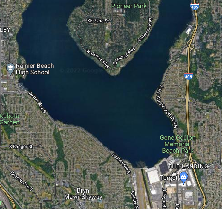
Figure 5: Lake Washington area.

Figure 6 illustrates the simulation state while tracking a HAB. As mentioned above and depicted at the bottom of Figure 4, at this stage of the project, all the measured data from the water body are from EEMS, except for the irradiance values that are taken from PVGIS since EEMS does not include these. The rest of the data (USVs battery status, bloom displacement prediction, etc.) come from our models. Next, we describe each plot in Figure 6:

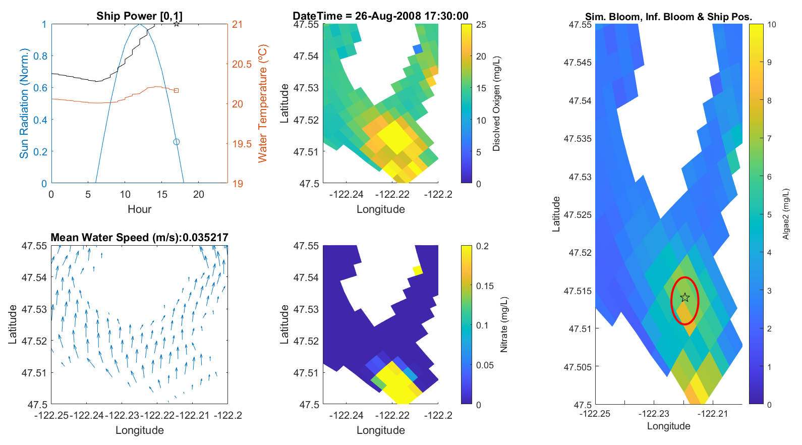
Figure 6: Frame of bloom tracking simulation: (upper-left) USV measured signals , water temperature, and solar irradiance, (lower-left) water speed. (top-center) oxygen density, (bottom-middle) nitrate density, (right) HAB EEMS given density for validation, HAB prediction as a red circle and ship position as a star.

• The upper left graph shows the signals measured by the USV and the irradiance sensor as a function of the time of day: sun radiation (blue), water Temperature (red), and ship’s electric power (black). At the time of the simulation, Figure 6 shows that the solar panels have fully charged the ship batteries.

• The lower left graph shows the map of water direction and velocity in the surface layer. The ship measures this signal at its position and reports it to the fog layer to estimate the bloom displacement. The simulator also uses the information from this map to perturb the ship dynamics.

• The top center graph shows the map of the dissolved oxygen density in the surface layer. The USV takes this measurement, and the inference model uses it to decide whether there is a bloom or not.

• The bottom middle graph shows the map of nitrate density on the surface. The inference model takes this measurement obtained by the USV to estimate the bloom growth.

• The right graph shows the HAB density map in the surface layer, the inferred bloom (red circle), and the USV position. The HAB density map is data directly taken from EEMS to validate that the inference model is correctly predicting the HAB dynamic.

The full simulation video can be found in Video2022 .

As mentioned above, all the data used in this simulation are synthetic. Consequently, all the sensors work on virtual mode, as DTs. When a sensor must take a measurement, it searches the database (the EEMS file or the irradiance database), modifies the signal according to its technical characteristics, and generates a message with the signal value. The fog layer receives these signals to perform different calculations like the model inference and periodically uploads them to the cloud layer. Figure 7 shows the signal values recorded by all the sensors of this use case after several (virtual) days of simulation.

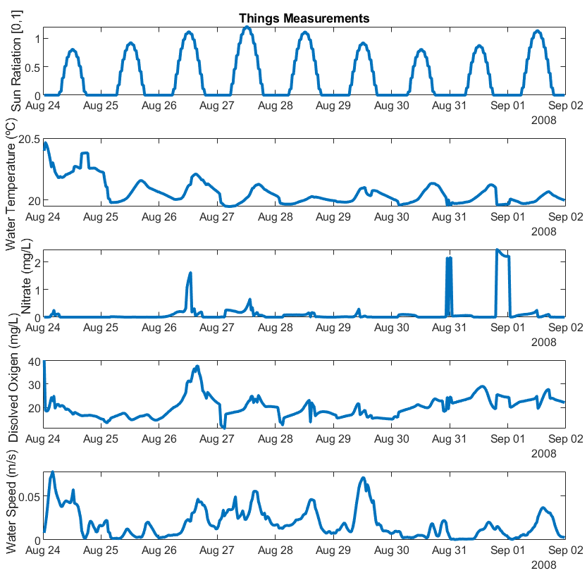
Figure 7: Sensors’ signals.

Figure 8 shows the evolution of the HAB inference model. The first plot shows a boolean value indicating whether the bloom has been detected or not. The second plot shows the estimated bloom density. The third and fourth plots show the displacement estimation: longitude and latitude. Figure 8 shows how blooms are detected and monitored almost every day. Some of these blooms have significant densities and move around significantly, requiring dynamic monitoring.

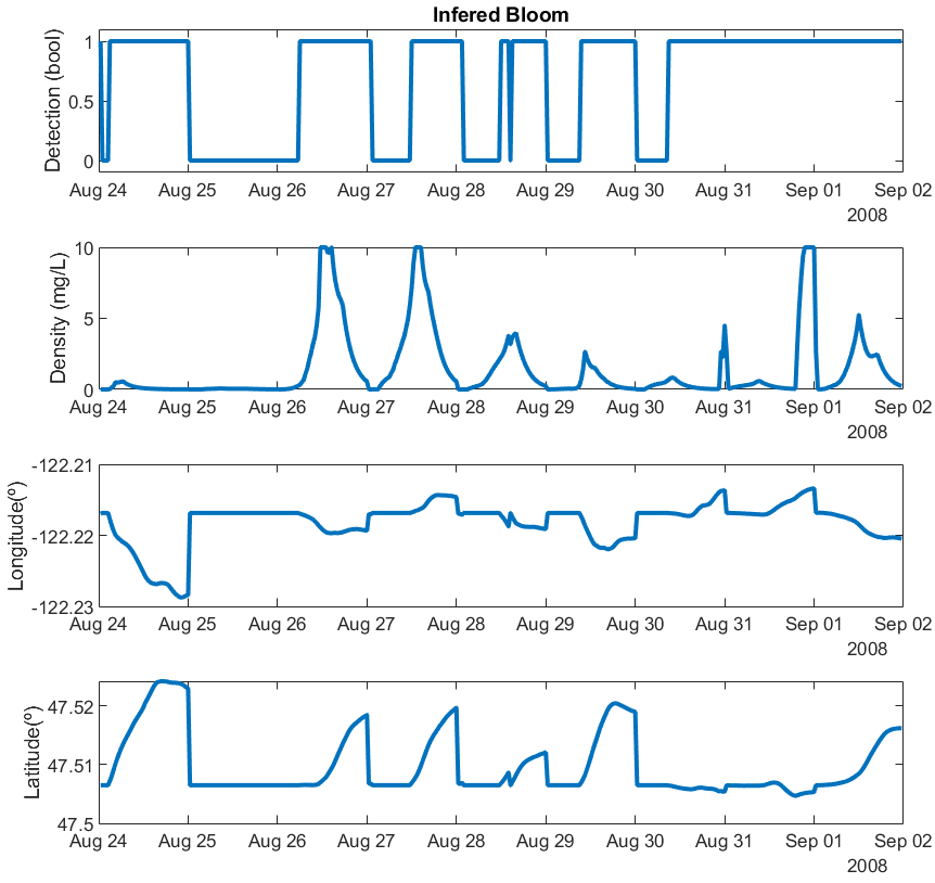
Figure 8: Bloom Inference model.

Finally, Figure 9 depicts the status of the USV model. The first graph shows the status of the power unit. The second plot shows the velocity of the USV. The third and fourth graphs show the position, longitude, and latitude. On August 30, the Figure shows that the USV runs out of battery since it has been tracking blooms to distant points for four consecutive days.

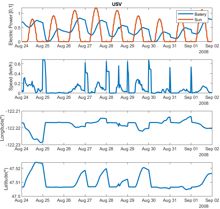
Figure 9: USV model.

4.2 Prediction use case

The second use case is relevant for water authorities. It consists of predicting HABs in the coming days based on weather forecasts. At the end of the day, the GCS in Figure 4 uploads all this information to the cloud layer. All the data history is available in this layer, allowing us to use the predictive model to analyze medium or long-term events.

To predict future blooms, a Prediction Service atomic model has been implemented in the cloud layer. This service is responsible for predicting the occurrence of upcoming HABs and their evolution from weather forecasts. These predictions depend highly dependent on local conditions, so they must be designed ad hoc. In our case, in this area of the lake, there is a source of nitrates or dissolved sediments, which is activated by rainfall. At ideal water temperatures, these dissolved sediments and the sunlight are the main precursors of HABs. From these precursors, bloom growth can be predicted. On the other hand, surface water currents can be inferred from wind forecasts, which can be used to predict the HAB displacement.

Firstly, the state of water and dissolved sediments are inferred from wind, sun, and rainfall forecasts. Figure 10 shows the results of this inference, comparing it with the results generated with EEMS. The first plot shows the rainfall forecast and the inference of dissolved sediments, which follows a simple exponential model. The second plot shows the bloom precursor signal, Sun-Nitrates, the values generated by EEMS and those inferred by the service. The third plot shows the wind forecast, and the fourth plot shows the inferred values for the water speed.

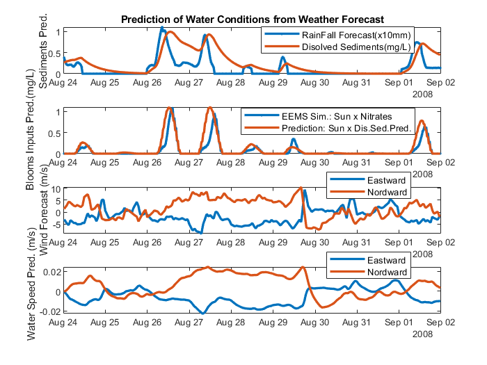
Figure 10: Water and dissolved sediments state inferreed from wind, sun and rainfall forecasts.

Next, the Prediction Service atomic model computes the HAB state from the previous results. Figure 11 shows the final output, comparing it to the results simulated with EEMS. The plot on the left shows the HAB density generated by EEMS versus the density predicted by the atomic model. It can be seen that it correctly predicts the 60% of the bloom cases. The graph on the right shows the trajectory of these HABs, predicting where the bloom will move accurately in most cases.

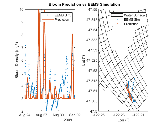
Figure 11: Bloom prediction.

4.3 Integration of real sensors and USV design

DEVS-BLOOM uses the xDEVS/Python library. xDEVS/Python can simulate models in real-time J-RiscoMartin2022b . A scaling factor can be provided, transforming hours into minutes, minutes into seconds, etc. This is important when incorporating hardware in the loop to the virtual frameworkNiyonkuru2021 since, for instance, the previous use case handles periods of 30 minutes, but we may want to perform tests with sensors sending data every minute. Additionally, xDEVS can interrupt the real-time simulation with the arrival of data sent by an external hardware device. To do this, the root coupled model must have an input port to inject data, and an atomic model must handle the arrival of this data through its external transition function.

To demonstrate the ability of DEVS-BLOOM to integrate actual sensors, we have used the xDEVS characteristics mentioned above with the irradiance sensor. Figure 12(a) depicts schematically how the real sensor is connected to the original atomic model shown in Figure 4. To this end, we use the input port $d_{i}$ explained in Figure 2, adding an input $d_{i}$ port to the root coupled model. xDEVS/Python automatically manages the communication between the sensor and DEVS-BLOOM through a software handler. The procedure is relatively straightforward since the external transition function of the sensor DT is automatically triggered when the actual sensor injects data.

On the other hand, Figure 12(b) shows a picture of a real-time execution, where data received by the actual sensor is correctly logged by DEVS-BLOOM. This procedure also allows us to validate the virtual sensor model, tuning its parameters (delay, precision, noise, etc.) if necessary. The predictive algorithms automatically manage failures in sensors. There is an outliers detection phase before the prediction, where outliers and missing data are replaced by regression. An alarm is triggered in case of failure, and the domain expert can take action if necessary. The parallel DEVS formalism is of great help when dealing with these issues.

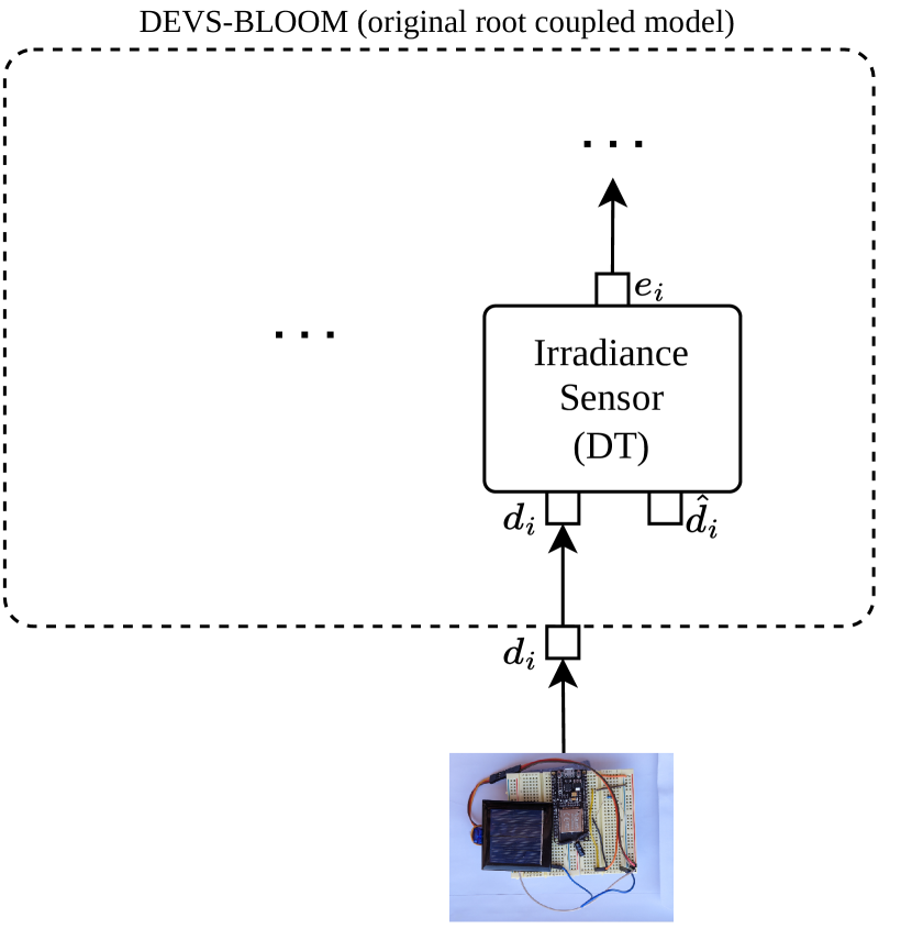
(a) Integration scheme of an actual sensor in DEVS-BLOOM.

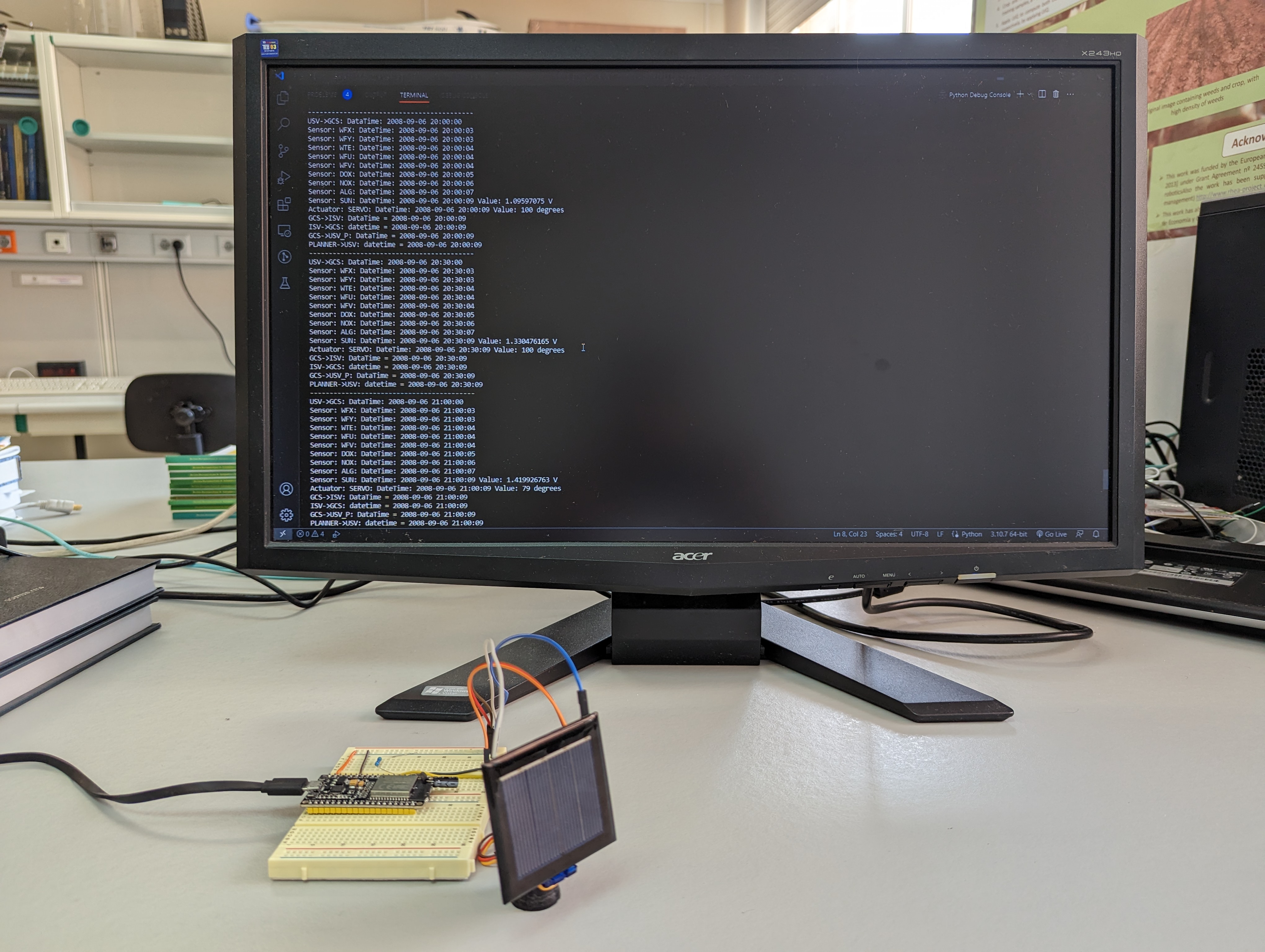
(b) DEVS-BLOOM real-time simulation with the actual sensor.

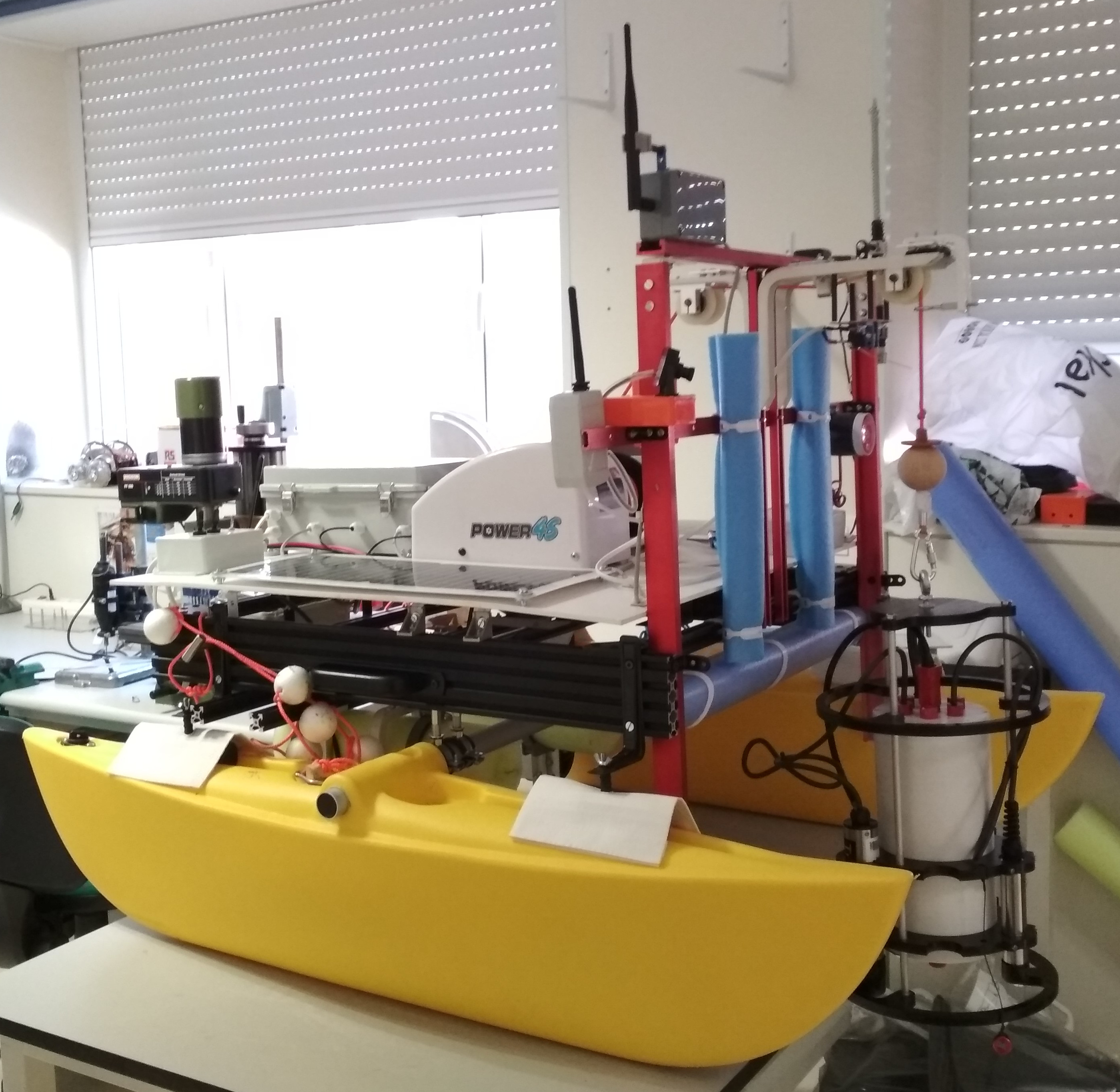
(c) USV first prototype.

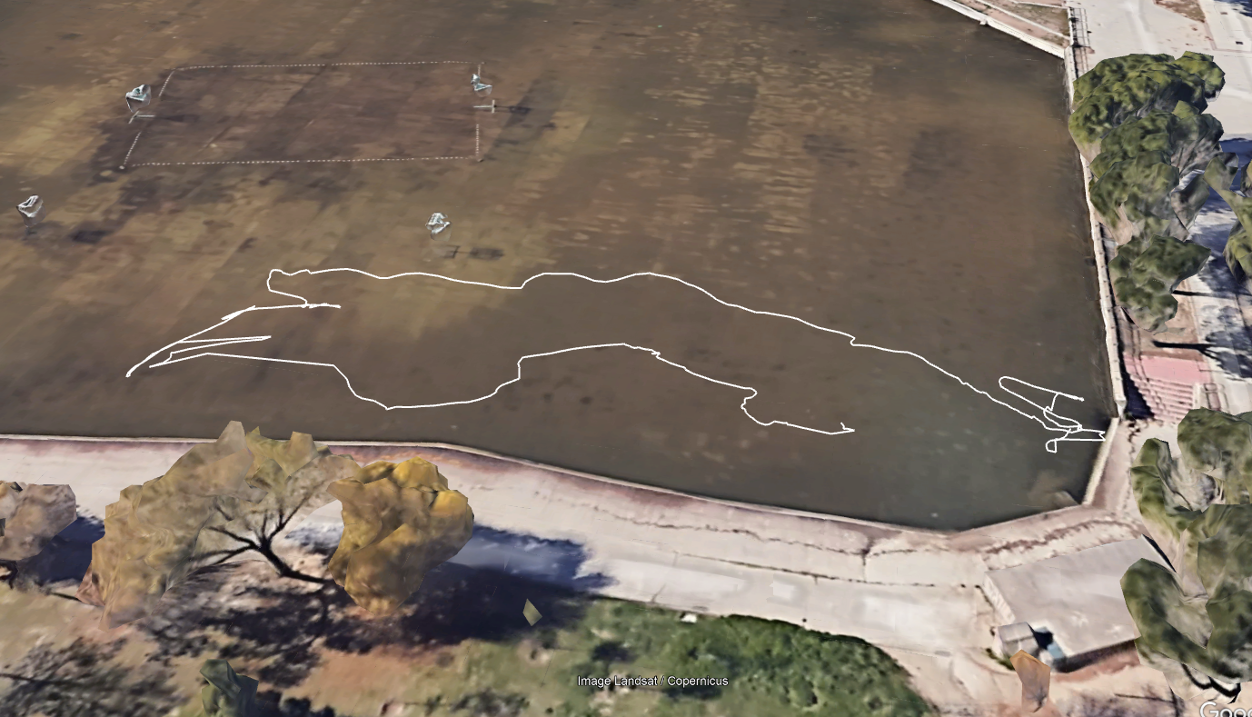
(d) Trajectory registered by the USV in a navigation test.

Figure 12: Integration of real sensors and USV design.

New sensors are acquired and tested through our framework as the project evolves. Currently, the most challenging part is the USV design. Figure 12(c) shows our first USV prototype with all the sensors embedded, and Figure 12(d) depicts one of the controlled tests to validate the navigation system. As the USV evolves, the DEVS-BLOOM virtual model does the same to match the behavior of the real counterpart FerreroLosada2023 .

As it can be seen, DEVS-BLOOM can help us to design an integral EWS considering different elements and exploring all the alternatives. Our M&S framework facilitates the elaboration of sustainable and efficient HAB management systems while saving costs with well-dimensioned instruments, USVs, and GCSs.

5 Conclusion and future work

HABs induce severe threats to water quality. To properly detect, assess, and mitigate these threats to water infrastructures, it is necessary to envision well-structured and robust methods to perform continuous monitoring and to deploy efficient infrastructure and proactive strategies to reduce their adverse effects. CPS integrative M&S is crucial to reaching these objectives since it provides sustainable mechanisms to analyze algorithms and the infrastructure we may need to deploy such systems. However, current approaches do not combine the analysis of base models and algorithms with the infrastructure.

In this paper, we have introduced DEVS-BLOOM, a novel M&S framework to enable real-time monitoring and hazard prediction of HABs while analyzing the effectiveness of infrastructure deployment. Our framework can automatically manage the design of advanced EWSs and propose decisions over the evolution of HABs. Our approach is based on solid principles of MBSE and the DEVS M&S formalism. Furthermore, the entire infrastructure can be modeled upon the IoT and DT paradigms. DEVS-BLOOM allows an incremental design, assuring reliability and scalability to multiple water bodies and minimizing costs in the conception of the final installations. Additionally, all the predictive models designed in the M&S phase can be later used in the real infrastructure. Our framework also allows different resolution views, for the interpretation of a domain expert at the fog layer and the interpretation of water authorities at the cloud layer, following the IoT nomenclature.

Future work includes, on the one hand, the inclusion of new models (e.g., related to the USVs dynamics) into DEVS-BLOOM, the improvement of its visualization tools, or the validation of the current HAB models against a real scenario. On the other hand, we plan to incrementally replace all the elements in the simulated model with those in a real-world use case, complementing the virtual representation of the system introduced in this paper with its final deployment.

Finally, we want to highlight that having a scientific framework to predict HABs formation and to take management actions also provides an organizing principle for fundamental research. This framework will serve and benefit the engagement of theory with M&S foundations. Complementary HAB research on mathematical models or systems engineering can be easily integrated into our DEVS-BLOOM framework. It will improve the scientific exploitation of discoveries and support the development of new bases for forecasting future effects on water quality and other sustainable water ecological challenges such as wastewater recycling or smart agriculture.

The authors would like to thank Mr. Giordy Alexander Andrade Aimara, who implemented the integration of actual sensors into DEVS-BLOOM as part of his master’s thesis. This work has been supported by the Research Projects IA-GES-BLOOM-CM (Y2020/TCS-6420) of the Synergic program of the Comunidad Autónoma de Madrid, SMART-BLOOMS (TED2021-130123B-I00) funded by MCIN/AEI/10.13039/501100011033 and the European Union NextGenerationEU/PRTR, and INSERTION (PID2021-127648OB-C33) of the Knowledge Generation Projects program of the Spanish Ministry of Science and Innovation.

José L. Risco-Martín received his Ph.D. from UCM, where he currently is Full Professor in the Department of Computer Architecture and Automation. His research interests include systems modeling, simulation, and optimization.

Segundo Esteban is an Associate Professor of Systems Engineering and Automation at UCM. He holds a Ph.D. in Physics from the same University. His research interests include Systems Modeling and Control.

Jesús Chacón is an Assistant Professor in the Faculty of Physics Sciences at Universidad Complutense de Madrid. He holds a Ph.D. in Physics from the same University. His research interests include modeling, simulation and implementation of event-based control systems, and education in control engineering.

Gonzalo Carazo-Barbero is a PhD student in Faculty of Informatics at Universidad Complutense de Madrid. His research interests include modeling and simulation of cyanobacterial blooms and unmanned surface vehicles path planning.

Eva Besada-Portas is an Associate Professor of Systems Engineering and Automation at UCM. She also holds a PhD in Computer Systems from UCM. Her research interests include uncertainty modeling and simulation, optimal control and planning of unmanned vehicles.

José A. López-Orozco is a Full Professor in the UCM. He holds a Ph.D. in Physics from the same University. His research interests include multisensor data fusion, control and planning of unmanned vehicles, and robotics.

References

- (1) Vincent WF. Cyanobacteria. Encyclopedia of Inland Waters 2009; 3: 226–232.
- (2) Schmale DG, Ault AP, Saad W et al. Perspectives on Harmful Algal Blooms (HABs) and the cyberbiosecurity of freshwater systems. Frontiers in Bioengineering and Biotechnology 2019; 128.
- (3) Meriluoto J, Spoof L and Codd GA. Handbook of cyanobacterial monitoring and cyanotoxin analysis. John Wiley & Sons, 2017.
- (4) Ung MT and Moellmer WO. A practical example of the use of simulation to develop an optimal plan for water—quality control. SIMULATION 1972; 19(4): 109–117. 10.1177/003754977201900402. URL https://doi.org/10.1177/003754977201900402. https://doi.org/10.1177/003754977201900402.
- (5) Long TY, Wu L, Meng GH et al. Numerical simulation for impacts of hydrodynamic conditions on algae growth in Chongqing section of Jialing river, China. Ecological Modelling 2011; 222(1): 112–119. 10.1016/j.ecolmodel.2010.09.028. URL https://www.sciencedirect.com/science/article/pii/S0304380010004990.
- (6) Pyo J, Duan H, Baek S et al. A convolutional neural network regression for quantifying cyanobacteria using hyperspectral imagery. Remote Sensing of Environment 2019; 233: 111350. 10.1016/j.rse.2019.111350. URL https://www.sciencedirect.com/science/article/pii/S0034425719303694.
- (7) DSI. EE Modeling System. https://www.eemodelingsystem.com, 2022. URL https://www.eemodelingsystem.com/user-center/downloads.
- (8) Wu Y, Zhang J, Hou Z et al. Seasonal dynamics of algal net primary production in response to phosphorus input in a mesotrophic subtropical plateau lake, southwestern China. Water 2022; 14(5).
- (9) Wymore AW. Model-based systems engineering, volume 3. CRC press, 2018.
- (10) Zeigler BP, Muzy A and Kofman E. Theory of modeling and simulation: discrete event & iterative system computational foundations. Academic press, 2018.
- (11) Marcosig EP, Giribet JI and Castro R. DEVS-OVER-ROS (DOVER): A framework for simulation-driven embedded control of robotic systems based on model continuity. In 2018 Winter Simulation Conference (WSC). pp. 1250–1261. 10.1109/WSC.2018.8632504.
- (12) Vinçon-Leite B and Casenave C. Modelling eutrophication in lake ecosystems: a review. Science of the Total Environment 2019; 651: 2985–3001.
- (13) Van Sebille E, Griffies SM, Abernathey R et al. Lagrangian ocean analysis: Fundamentals and practices. Ocean Modelling 2018; 121: 49–75.
- (14) Chen Y, Song L, Liu Y et al. A review of the artificial neural network models for water quality prediction. Applied Sciences 2020; 10(17): 5776.
- (15) Rousso BZ, Bertone E, Stewart R et al. A systematic literature review of forecasting and predictive models for cyanobacteria blooms in freshwater lakes. Water Research 2020; 182: 115959.
- (16) DHI. MIKE ECO Lab, 2022. URL https://www.mikepoweredbydhi.com/products/mike-eco-lab. (Visited on 11/2022).
- (17) Deltares. Delft3D 4, 2022. URL https://oss.deltares.nl/web/delft3d. (Visited on 11/2022).
- (18) Vélez C, Alfonso L, Sánchez A et al. Centinela: an early warning system for the water quality of the Cauca river. Journal of Hydroinformatics 2014; 16(6): 1409–1424.
- (19) Silva A, Pinto L, Rodrigues S et al. A HAB warning system for shellfish harvesting in Portugal. Harmful Algae 2016; 53: 33–39.
- (20) Serramiá A. SAIH/SAICA: automatic hydrological information system and automatic water quality information system in the Spanish watersheds. Tecno Ambiente (España) 2004; 139: 15–18.
- (21) Shoutheast Environmental Research Center. SERC water quality monitoring network, 2022. URL http://serc.fiu.edu/wqmnetwork/. (Visited on 11/2022).
- (22) Riskin ML and Lee CJ. U.S. Geological Survey National Water Quality Monitoring Network. Technical report, USGS National Water Quality Monitoring Network, Reston, VA, 2021. 10.3133/fs20213019.
- (23) ECCC. Overview of freshwater quality monitoring and surveillance, 2022. URL https://www.canada.ca/en/environment-climate-change/services/freshwater-quality-monitoring/overview.html. (Visited on 11/2022).
- (24) Basha EA, Ravela S and Rus D. Model-based monitoring for early warning flood detection. In Proceedings of the 6th ACM Conference on Embedded Network Sensor Systems. SenSys ’08, New York, NY, USA: Association for Computing Machinery. ISBN 9781595939906, p. 295–308. 10.1145/1460412.1460442. URL https://doi.org/10.1145/1460412.1460442.
- (25) Curl JM, Nading T, Hegger K et al. Digital twins: the next generation of water treatment technology. Journal-American Water Works Association 2019; 111(12): 44–50.
- (26) Henares K, Risco-Martín JL, Ayala JL et al. Efficient micro data centres deployment for mobile healthcare monitoring systems in iot urban scenarios. Journal of Simulation 2022; : 1–15.
- (27) Cárdenas R, Arroba P and Risco-Martín JL. Bringing AI to the edge: A formal M&S specification to deploy effective IoT architectures. Journal of Simulation 2021; 16(5): 494–511. 10.1080/17477778.2020.1863755.
- (28) Risco-Martín JL, Mittal S, Henares K et al. xDEVS: A toolkit for interoperable modeling and simulation of formal discrete event systems. Software: Practice and Experience 2022; : 1–4210.1002/spe.3168.
- (29) Risco-Martín JL, Henares K, Mittal S et al. A unified cloud-enabled discrete event parallel and distributed simulation architecture. Simulation Modelling Practice and Theory 2022; 118.
- (30) Herguedas-Pinedo B, Risco-Martín JL, Esteban S et al. Predictive modeling and simulation system for the management of harmful cyanobacteria blooms. In Proceedings of the 2023 Annual Modeling and Simulation Conference (ANNSIM’23).
- (31) Esteban S. HAB Monitoring Simulation Video, 2022. URL https://archive.org/details/habsim-20220920.
- (32) Niyonkuru D and Wainer G. A DEVS-based engine for building digital quadruplets. SIMULATION 2021; 97(7): 485–506. 10.1177/00375497211003130. URL https://doi.org/10.1177/00375497211003130. PMID: 34219819, https://doi.org/10.1177/00375497211003130.
- (33) Ferrero-Losada S, Besada-Portas E, Risco-Martín JL et al. DEVS-based modeling and simulation of data-driven exploration algorithms of lentic water bodies with an ASV. In Proceedings of the 2023 Annual Modeling and Simulation Conference (ANNSIM’23).