Compact Pulse Schedules for High-Fidelity Single-Flux Quantum Qubit Control

Abstract

In the traditional approach to controlling superconducting qubits using microwave pulses, the field of pulse shaping has emerged in order to assist in the removal of leakage and increase gate fidelity. However, the challenge of scaling microwave control electronics has created an opportunity to explore alternative methods such as single-flux quantum (SFQ) pulses. For qubits controlled by SFQ pulses, high fidelity gates can be achieved by optimizing the binary control sequence. We extend the notion of the derivative removal by adiabatic gate (DRAG) framework a transmon qubit controlled by SFQ drivers and propose pulse sequences that can be stored in 22 bits or fewer, with gate fidelities exceeding 99.99%. This modest memory requirement could help reduce the footprint of the SFQ coprocessors and power dissipation while preserving their inherent advantages of scalability and cost-effectiveness.

I Introduction

Superconducting qubits are a promising architecture for quantum computation, demonstrating high fidelities, long coherence times, and scalability to hundreds of qubits [1, 2]. However, scaling to thousands of qubits, required for fault-tolerant computation, remains an experimental challenge, with heat dissipation issues and rising costs [3]. Using single-flux quantum (SFQ) pulses to control a qubit’s state has been proposed as an alternative to traditional microwave drives [4, 5]. In this scheme, voltage pulses whose integrated area equates to a superconducting flux quantum $\Phi=h/2e$ are delivered to the qubit [6, 7], controlled by a classical coprocessor integrated into the chip. Such an architecture is very robust and expends significantly less power, leading to fewer heating issues and allowing for much greater scalability [8, 9], making is a strong candidate for noisy, intermediate-scale quantum era devices. Further, all of the pulses irradiating the qubit are precisely equivalent, allowing for reliable control. However, due to quasiparticle poisoning, this digital control of qubits typically lags behind their microwave counterpart in precision, with experimental single-qubit gate fidelities ranging from 95%–98% [10, 11, 12]. This limited fidelity is expected to be addressed in future iterations of the architecture [5].

Traditionally, control of a qubit is conducting using a sequence of evenly spaced SFQ pulses, referred to as a “pulse train” [10]. While this scheme is simple and easy to implement, the fidelity of operations is generally limited by leakage [13]. Consequently, there has been an increase in literature on optimal schemes to control these qubits, with genetic and trust-region algorithms proposed [13, 14]. Gates implemented with such optimized pulse sequences are predicted to have fidelities as high as $99.99\%$, on par with microwave gate methods. However, these sophisticated pulse sequences face higher memory requirements than pulse trains, as the pulses must be encoded as a binary sequence on a bit-shift register [15], which functions as the coprocessor memory. Minimizing memory requirements is of paramount importance for SFQ-based technologies, resulting in a reduction in the power dissipation and along with it the footprint of the coprocessor [5]. In order to reduce hardware requirements, it is possible to tailor schemes to be “hardware efficient”, requiring fewer bits to encode a sequence, with proposed methods resulting in similar fidelities, but with a reduction in the bit requirements from 250 to fewer than 55 [16].

On most larger-scale superconducting architectures, such as on state-of-the-art surface codes [17, 18], pulses optimized via gradient descent [19] are generally not used due to their complexity and the challenges of closed-loop optimization. Instead, the derivative removal by adiabatic gate (DRAG) pulse shaping technique is used ubiquitously for single- and two-qubit gates, due to its simple implementation and performance [20]. In this work, we propose a digital analog to the DRAG framework, which implements arbitrary single-qubit rotations with fidelities exceeding 99.99%. As the majority of the pulses are simply an SFQ train, this greatly reduces the memory requirements for encoding the pulse sequences, with at most 22 bits required for implementation.

The paper is organized as follows. In Section II, we present a model for the SFQ pulses using a transmon superconducting qubit. In Section III, we provide details on the discrete equivalent of DRAG pulses, with analogies to the continuous model, and discuss the encoding of the pulses in Section IV. In Section V, we report the results and fidelities of this pulse scheme and demonstrate its robustness against parameter variations. Section VI concludes the paper.

II A Model for SFQ Control

We consider the model for the transmon qubit [21]

$$\widehat{H}_{0}=4E_{C}(\hat{n}-n_{g})^{2}-E_{J}\cos{\hat{\varphi}}\,,$$ (1)

where $E_{C}$ and $E_{J}$ are the charging and Josephson energies, respectively, and $n_{g}$ is the offset gate charge. In the regime $E_{J}\gg E_{C}$, the lowest-lying energy levels become exponentially insensitive to $n_{g}$; we thus take $n_{g}=0$ for simplicity. This Hamiltonian can be expanded in the Fock basis, yielding the approximate model

$$\widehat{H}_{0}\approx\omega_{q}\hat{b}^{\dagger}\hat{b}-\frac{\alpha}{2}\hat{b}^{\dagger 2}\hat{b}^{2},$$ (2)

with the qubit frequency $\omega_{q}\approx\sqrt{8E_{C}E_{J}}$, the anharmonicity $\alpha\approx-E_{C}$, and $\hat{b}^{\dagger}$ and $\hat{b}$ are the creation and annihilation operators of the transmon, respectively. Unless otherwise mentioned, we assume that $\omega_{q}/2\pi=5$ GHz and $\alpha/2\pi=250$ MHz, corresponding to the ratio $E_{J}/E_{C}\approx 69$.

II.1 Qubit Control by Continuous Driving

Transmon qubits are traditionally driven using a charge line. The charge operator in the Fock basis can be represented as

$$\hat{n}\approx\frac{i}{2}\left(\frac{E_{J}}{2E_{C}}\right)^{\frac{1}{4}}(\hat{b}^{\dagger}-\hat{b})=ir(\hat{b}^{\dagger}-\hat{b}),$$ (3)

where $r$ is the magnitude of the zero-point fluctuations of the charge operator. Time-dependent control of the transmon qubit can thus be represented with the Hamiltonian

$$\widehat{H}(t) =\widehat{H}_{0}+\widehat{H}_{\mathrm{D}}(t),$$ (4)

where $\widehat{H}_{\mathrm{D}}(t)=i\Omega(t)(\hat{b}^{\dagger}-\hat{b})$ is the drive Hamiltonian and $\Omega(t)$ is a time-dependent pulse. In general, this pulse consists of a slowly varying pulse envelope, and a fast carrier frequency targeting the qubit transition, $\Omega(t)=\Omega_{0}(t)\cos(\omega_{q}t+\phi)$, where $\phi$ determines the axis of rotation around the Bloch sphere and $\int_{0}^{t}\Omega_{0}(t^{\prime})dt^{\prime}$ is the angle through which the qubit state is rotated. Then, entering a rotating frame $\widehat{U}=\exp(i\omega_{q}\hat{b}^{\dagger}\hat{b}t)$ and assuming $\phi=0$, we find the Hamiltonian

$$\widehat{H}^{\prime}(t)=-\frac{\alpha}{2}\hat{b}^{\dagger 2}\hat{b}^{2}+\frac{i}{2}\Omega_{0}(t)\left[\hat{b}^{\dagger}(1+e^{2i\omega_{q}t})-\hat{b}(1+e^{-2i\omega_{q}t})\right].$$ (5)

Then, the fast oscillatory terms $e^{2i\omega_{q}t}$ are dropped, yielding a rotating-wave approximation (RWA) Hamiltonian

$$\widehat{H}_{\textrm{RWA}}^{\prime}(t)=-\frac{\alpha}{2}\hat{b}^{\dagger 2}\hat{b}^{2}+\frac{i}{2}\Omega_{0}(t)(\hat{b}^{\dagger}-\hat{b}).$$ (6)

If the ratio $\Omega_{0}/\alpha$ is sufficiently small, the leakage level $|2\rangle$ of the transmon will be only weakly populated during the operation of the gate. Population of this leakage level can be reduced by pulse shaping, which is discussed in Section III.

II.2 Qubit Control Using SFQ Pulses

We now consider a different regime of qubit control: a sequence of discrete, fast pulses on the transmon qubit. Figure 1 shows a circuit diagram of an SFQ-driven qubit. It has been demonstrated that such pulses can be accurately modelled with a Dirac delta function [4]. As such, an SFQ pulse can be well-approximated by

$$\widehat{U}_{\textrm{kick}}(\theta)=\exp(-\frac{\theta}{2}\left[\hat{b}^{\dagger}-\hat{b}\right]),$$ (7)

where the kick angle $\theta=C_{c}\Phi_{0}\sqrt{2\omega_{q}/\hbar C}$. Here, $C$ is the self-capacitance of the qubit, $C_{c}$ is the capacitance between the qubit and the SFQ driver, and $\omega_{q}$ is the qubit frequency [4]. In this work, we consider a kick angle $\theta=0.03$.

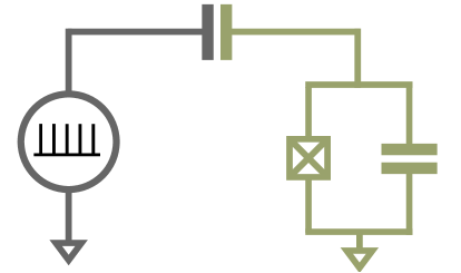
Figure 1: Transmon qubit (green) capacitvely coupled to the SFQ generator. We approximate the arrival of the pulses at the qubit as Dirac delta functions, resulting in a pulse train.

The unitary evolution of the qubit can be described as a series of operations—the free evolution of the qubit and the SFQ kick operators:

$$\widehat{U}=\prod_{i=0}^{N}\exp(-i\widehat{H}_{0}t_{i})\widehat{U}_{\textrm{kick}},$$ (8)

where $N$ is the total number of kicks and $t_{i}$ is the time interval between the $i$-th and $(i+1)$-th kick. Within a two-level approximation, we note that

$$\exp(-i\widehat{H}_{0}T)\widehat{U}_{\textrm{kick}}\approx\widehat{R}_{Y}(\theta).$$ (9)

where the qubit period $T=2\pi/\omega_{q}$. Consequently, by choosing all waiting times $t_{i}$ to be equal to the qubit period, we can approximate arbitrary $Y$ rotations around the Bloch sphere by applying a pulse train, where $\widehat{R}_{Y}(\theta_{\textrm{target}})\approx\widehat{R}_{Y}(n\theta)$.

II.3 Continuous Drive Equivalence to SFQ Kicks

We show here that the SFQ and continuous pictures are equivalent within the RWA. We first recall the Dirac comb function

$${}_{\phi,T}(t)=\sum_{n=-\infty}^{\infty}\delta(t-nT-\phi),$$ (10)

which approximates the SFQ pulse train, where $\phi$ is a phase offset. This results in the effective Hamiltonian

$$\widehat{H}(t)=\widehat{H}_{0}+\frac{i\theta}{2}{}_{0,(2\pi/\omega_{q})}(t)(\hat{b}^{\dagger}-\hat{b}),$$ (11)

which, when exponentiated, yields Eq. 8, with all waiting times $t_{i}=2\pi/\omega_{q}$. Making use of the identity

$${}_{\phi,(2\pi/\omega_{q})}(t)\equiv\frac{\omega_{q}}{2\pi}\sum_{n=-\infty}^{\infty}e^{-in(\omega_{q}t+\phi)},$$ (12)

and once again entering a rotating frame, yields the Hamiltonian

$$\widehat{H}^{\prime}(t) =-\frac{\alpha}{2}\hat{b}^{\dagger 2}\hat{b}^{2}+H_{\mathrm{D}}^{\prime}(t),$$ (13)

$$H_{\mathrm{D}}^{\prime}(t) =\frac{i\omega_{q}\theta}{4\pi}\hat{b}^{\dagger}\sum_{n=-\infty}^{\infty}e^{-in(\omega_{q}t+\phi)}+\textrm{H.c.}$$

Once again making an RWA, this time ignoring terms oscillating at $e^{\pm i\omega_{q}t}$ or faster, we return to the RWA form of the Hamiltonian in Eq. 6, and thus directly relate the drive amplitude and kick angle

$$\Omega_{0}(t)=\omega_{q}\theta/2\pi,$$ (14)

demonstrating the equivalence between the continuous drive and SFQ pictures.

III Leakage Removal via Ramps

The DRAG framework is used ubiquitously in superconducting qubit architectures to mitigate the effects of leakage errors [20]. By augmenting a given pulse shape $\Omega(t)$ with its time derivative, leakage effects can be greatly reduced. Consider the pulse shape

$$\Omega^{\prime}(t)=\Omega(t)+\frac{ic\dot{\Omega}}{\alpha},$$ (15)

where $c$ is a scalar. Figure 2(a) shows an illustration of a DRAG pulse, with the blue curve corresponding to the primary pulse $\Omega(t)$ and the orange curve to the derivative $\dot{\Omega}(t)$. The choice of $c=1$ effectively eliminates the spectral component of the pulse at the leakage frequency, as can be seen from the Fourier transform of the pulse over the gate time $T_{\mathrm{g}}$ [22]:

$$S(\Omega,\alpha) =\int_{0}^{T_{\mathrm{g}}}\Omega(t)e^{-i\alpha t}dt=-i\int_{0}^{T_{\mathrm{g}}}\frac{\dot{\Omega}(t)}{\alpha}e^{-i\alpha t}dt.$$ (16)

The relative phase difference $(-i)$ between the two terms in Eq. 16 is equivalent to a $\pi/2$ phase shift in the driving field:

$$\widehat{H}(t)=\widehat{H}_{0}+i(\hat{b}^{\dagger}-\hat{b})\left(\Omega(t)\cos(\omega_{q}t)+\frac{c\dot{\Omega}(t)}{\alpha}\sin(\omega_{q}t)\right).$$ (17)

Figure 2: Example pulse shapes for implementing an $\widehat{R}_{Y}(\theta)$ gate in microwave and SFQ architectures. (a) Example tanh pulse envelope (blue) microwave drive, with accompanying pulse derivative (orange), implemented on the opposing quadrature for DRAG. (b) Dirac delta approximation to the envelopes in (a), valid within the RWA. (c) Example SFQ pulse sequence, inspired by the sequence in (b). Here, the kick angle is fixed. Negative weighting on kicks can be effectively implemented by shifting the delta function by $T/2$.

We consider a mapping from the DRAG formalism to an equivalent SFQ interpretation. As is standard practice, we assume the drive pulse $\Omega(0)=\Omega(T_{\mathrm{g}})=0$ is zero at the start and end of the gate, with gate time $T_{\mathrm{g}}$. Within the RWA made in the previous section, the drive Hamiltonian is equivalent to

$$\widehat{H}_{\mathrm{D}}(t)=\frac{i}{2}(\hat{b}^{\dagger}-\hat{b})$$ (18)

$$\times\left[\Omega_{y}(t){}_{0,2\pi/\omega_{q}}(t)+\Omega_{x}(t){}_{\pi/2,2\pi/\omega_{q}}(t)\right],$$

where

$$\Omega_{y}(t)=\frac{2\pi\Omega(t)}{\omega_{q}}\textrm{\,\, and \,\,}\Omega_{x}(t)=\frac{2c\pi\dot{\Omega}(t)}{\alpha\omega_{q}}.$$ (19)

We now consider the unitary corresponding to what is known as an “on-ramp”, where in the case of the microwave drive the amplitude is slowly increased. The equivalent SFQ evolution operator thus becomes

$$\widehat{U}_{\textrm{on}}(t_{\mathrm{r}}) =\mathcal{T}\exp(-i\int_{0}^{t_{\mathrm{r}}}[\widehat{H}_{0}+\widehat{H}_{\mathrm{D}}(t^{\prime})]dt^{\prime})$$ (20)

$$=\prod_{n}e^{-i3T/4}\widehat{U}_{\textrm{kick}}[\Omega_{x}(nT+T/4)]$$

$$\ \ \ \ \times e^{-iT/4}\widehat{U}_{\textrm{kick}}[\Omega_{y}(nT)],$$

where $t_{\mathrm{r}}$ refers to the “ramp time”, or the time it takes the pulse amplitude to reach its maximum value, $t_{\mathrm{r}}=\arg\max_{t}\Omega(t)$. An example pulse sequence corresponding to this unitary is given in Fig. 2(b), where each of the SFQ kicks takes on a different effective amplitude.

While the SFQ Hamiltonian in Eq. 18 is equivalent to the continuous drive in Eq. 17 up to an RWA, we require all the SFQ kick angles $\theta$ to be identical, as this is fixed by the circuit capacitances [10]. As such, we approximate the DRAG condition introduced in Eq. 15 by first equating the integrated pulses:

$$\Omega_{x} =c\frac{\dot{\Omega}}{\alpha}\rightarrow\int_{0}^{t_{\mathrm{r}}}\Omega_{x}(t)dt=\frac{c}{\alpha}{\Omega(t_{\mathrm{r}})}.$$ (21)

We quantize this relation, with $\int_{0}^{t_{\mathrm{r}}}\Omega_{x}(t)dt=n\theta$, where $n$ is the effective number of pulses in the $x$ direction. Using the relation in Eq. 14, we describe the target number of kicks in the $x$ direction as

$$n=\frac{c}{\alpha}T.$$ (22)

The goal is thus to find “SFQ ramps”, or specific sets of SFQ pulses, that implement Eq. 22. In this sense, the evolution of the system will be decomposed into three pieces: the on-ramp evolution, an SFQ “pulse train” corresponding to a set of SFQ kicks, and an “off-ramp” evolution, as depicted in Fig. 2(c):

$$\widehat{U}(T)=\widehat{U}_{\textrm{off}}(t_{\mathrm{r}})\widehat{U}_{\textrm{train}}\widehat{U}_{\textrm{on}}(t_{\mathrm{r}}).$$ (23)

In close analogy with analog DRAG pulses, the off-ramp $\widehat{U}_{\textrm{off}}(t_{\mathrm{r}})$ should be symmetric with respect to the on-ramp unitary along the $y$-axis and antisymmetric along the $x$-axis for the implementation of an $\widehat{R}_{Y}(\theta)$ gate. While we cannot control the sign of the amplitude of the kick, the equivalent $\widehat{R}_{X}(-\theta)$ rotation can be achieved by an effective shift of the arrival time of the pulses in the $x$ direction by $T/2$.

While the choice of $c=1$ minimizes leakage, it has been demonstrated that $c=0.5$ maximizes the gate fidelity due a reduction in phase errors [23]. Alternatively, DRAG can be coupled with a virtual $\widehat{Z}$ gate to suppress both phase and leakage [24, 25]. As the choice of the $c$ parameter is limited by the quantization relation in Eq. 22 and we cannot correct for arbitrary phase errors with a virtual $\widehat{Z}$ gate, we simply optimize the gate fidelity, as discussed in Section V.

IV Encoding the Pulse Sequence

The possible choices of SFQ ramps will depend on the SFQ global clock, which controls the arrival time of the pulses. Thus, to achieve the resonant pulse train, the SFQ clock frequency must be some integer multiple of the qubit frequency. We begin by assuming a clock frequency of 20 GHz, such that the period of the clock $T_{\mathrm{c}}=T/4$, which, as discussed in the previous section, is required for implementing the equivalent evolution to continuous dynamics. As such, by choosing pulses every four clock cycles, we can effectuate $\widehat{R}_{Y}(\theta)$ rotations. Let us adopt the binary notation $ijkl$, where $\{i,j,k,l\}\in\{0,1\}$, to represent a sequence that is sent to the SFQ driver. Each $1$ and $0$ refers to either the presence or absence of an SFQ kick, followed by a waiting time of $T/4$. As a simple example, the binary sequence $1000$ effectuates

$$1000\rightarrow e^{-i\widehat{H}_{0}T}\widehat{U}_{\textrm{kick}}=\widehat{R}_{Y}(\theta)$$ (24)

on the qubit subspace. Similarly, the choices $0100$, $0010$, and $0001$ effectuate $\widehat{R}_{X}(-\theta)$, $\widehat{R}_{Y}(-\theta)$, and $\widehat{R}_{X}(\theta)$ rotations, respectively. To demonstrate this more concretely, we consider the simplest possible SFQ ramp of $0100$. The evolution corresponding to Eq. 23 can thus be represented by the binary sequence (recalling that the binary sequence is read from left to right)

$$\widehat{U}(T)\longrightarrow(0100)+(1000)^{(N-1)}+(1)+(0010)$$ (25)

$$=\widehat{R}_{Y}(-\theta)\widehat{R}_{Z}(\pi/2)\widehat{R}_{Y}(\theta)\widehat{R}_{Y}(\left[N-1\right]\theta)\widehat{R}_{X}(-\theta)$$

$$=\widehat{R}_{X}(\theta)\widehat{R}_{Y}(N\theta)\widehat{R}_{X}(-\theta),$$

up to an $\widehat{R}_{Z}(\pi/2)$ rotation. To consider more-complex ramps, we concatenate up to a total of five binary sequences from the subset $(0000,\ 1000,\ 0100,\ 1100)$, which correspond to $\widehat{I},\widehat{R}_{Y}(\theta),\widehat{R}_{X}(-\theta)$, and $\widehat{R}_{X}(-\theta)\widehat{R}_{Y}(\theta)$, respectively. Consequently, a choice of $n$ qubit cycles for the ramp leads to a total of $4^{n}$ possible ramps. The ignored binary sequences implement rotations in the opposite direction indicated by the DRAG technique or against the targeted gate rotation. In Appendix B, we demonstrate that the optimized DRAG sequences greatly reduce the spectrum of the pulse sequence at the leakage frequency, in agreement with Eq. 16.

An advantage of SFQ hardware is the speed and accuracy at which pulses can be delivered to the qubit. Consequently, global clocks of 40 GHz or higher are feasible [26, 27]. For the provided choice of parameters, such a clock frequency would equate to eight times the qubit frequency, allowing for greater control of the qubit. In line with the above terminology, we additionally consider ramps for the “8$\times$” clock. There are eight cycles to consider:

$$00000000,\ 10000000,\ 01000000,\ 00100000,$$

$$11000000,\ 10100000,\ 01100000,\ 11100000.$$

The faster clock enables pulses, such as $01000000$, that result in an effective $\theta/\sqrt{2}$ kick in both the $x$ and $y$ quadratures, giving faster and more-precise control.

In the case of the proposed ramps, a significantly smaller number of bits is required than traditional methods [13, 14]. Given there are four choices of ramp per qubit cycle for the 4$\times$ clock and eight for the 8$\times$ clock, the on-ramp can be described by $2n$ and $3n$ bits, respectively, where $n$ is the number of qubit cycles in the on-ramp. The number of pulses in the pulse train $N$ could easily be represented in binary form with $\lceil\log_{2}N\rceil$ bits, and the encoding for the off-ramp can be recycled from the on-ramp. Consequently, a five-ramp cycle with 84 pulses in the pulse train can be implemented using only $10+7=17$ bits for the 20 GHz clock and $15+7=22$ bits for the 40 GHz clock, respectively. As shown in Section V, this is sufficient for implementing gates with greater than $99.99\%$ fidelity. By sharing the encoding of the ramps and pulse trains between neighbouring qubits in a larger-scale device, the effective bit requirement per qubit could be brought even lower using this technique.

V Gate Optimization Using Ramps

We now demonstrate the performance of the proposed SFQ pulse trains with appropriate ramps for relevant target angles. We restrict our analysis to targeting arbitrary $y$ rotations, with target operators of the form

$$\widehat{U}_{\textrm{target}}=\cos(\theta_{\textrm{target}}/2)\widehat{I}-i\sin(\theta_{\textrm{target}}/2)\widehat{Y}.$$ (26)

We note that the equivalent $\widehat{R}_{X}(\theta)$ rotations can be achieved using $(0001)^{N}$ pulse trains. To quantify the gate performance in the presence of leakage, we use the average gate fidelity metric in the absence of a loss channel [25]:

$$\overline{F}(\mathcal{E})=\frac{2F_{\textrm{pro}}(\mathcal{E})+1-L_{1}}{3}.$$ (27)

Here, the process fidelity is defined as

$$F_{\textrm{pro}}(\mathcal{E})=\frac{1}{4}\left|\Tr[\widehat{U}^{\dagger}_{\textrm{target}}\widehat{U}_{Q}]\right|^{2},$$ (28)

and the leakage metric is

$$L=1-\frac{1}{2}\Tr(\widehat{U}_{Q}\widehat{U}^{\dagger}_{Q}),$$ (29)

where $\widehat{U}_{Q}$ is the projection onto the computation subspace of the full unitary operation $\widehat{U}$ (see Eq. 23), which takes into account the higher-energy levels and leakage effects. To ensure the numerical accuracy of our work, we consider the full-cosine Hamiltonian of the transmon in Eq. 1, diagonalized in the charge basis with 200 states and projected onto the lowest seven eigenstates. This ensures that the simulations will capture additional leakage to the $|3\rangle$ state and higher transmon eigenstates. Further, the kick operator is taken as the exponential of the charge operator:

$$\widehat{U}_{\textrm{kick}}(\theta)=\exp(-\frac{\theta^{\prime}}{2}\hat{n}),$$ (30)

where $\theta^{\prime}=\theta/r$, accounting for the zero-point fluctuations of the charge operator $\hat{n}$. We consider the performance of this method with a finite qubit lifetime in Appendix A.

To find the optimal ramps, we perform an exhaustive search over relevant ramps that maximize $\overline{F}(\mathcal{E})$ for each target gate $\widehat{R}_{Y}(\theta)$. As we consider a maximum of five cycles, all possible ramps can easily be tested. For longer ramps and more-complex systems, a combination of the constraint in Eq. 22 and the pulse sequence spectrum (see Appendix B) can be used to reduce the possible ramp subspace and accelerate the optimization. In Fig. 3, we plot the fidelity of operation of a target rotation $\widehat{R}_{Y}(\theta)$ as a function of the target angle for the 4$\times$ clock. The different colours represent differing numbers of on-ramp and off-ramp cycles, with blue (0 cycles) representing only a pulse train. As expected, the longer ramps yield significantly higher fidelities, with four cycles yielding less than an error of $10^{-4}$ for most target angles. However, we note that the fidelity is eventually limited for four cycles, with almost identical fidelities for five cycles.

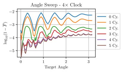
Figure 3: Maximum fidelity of target rotation operations $\widehat{R}_{Y}(\theta)$ as a function of the target angle. The optimal pulse train length and optimal ramp for each ramp length is postselected.

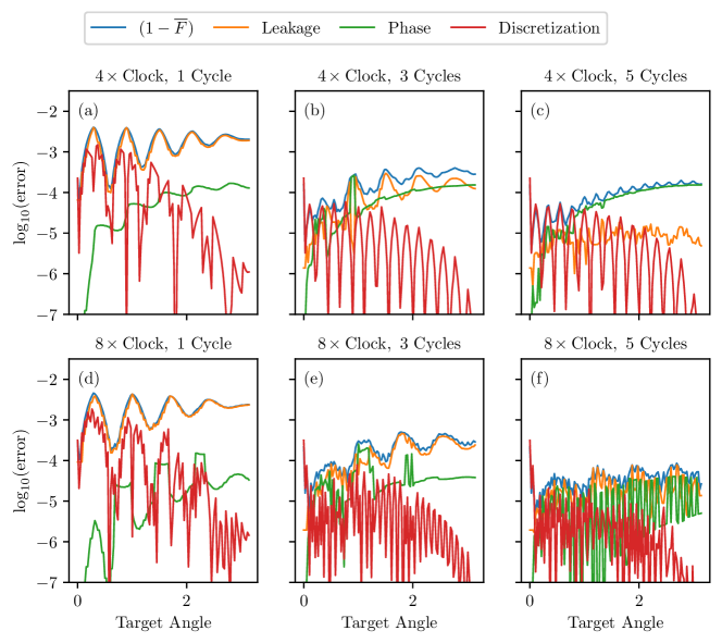
Figure 4: Error analysis for the 4$\times$ clock (a)–(c) and 8$\times$ clock (d)–(f). For the shorter ramps, the leakage remains the dominant source of error, but is significantly suppressed with a five-cycle on-ramp. For small target angles, the discretization error dominates. For larger angles, the phase error dominates.

In order to gain greater insight into the source of the errors, it is useful to perform a decomposition of the projected operator $\widehat{U}_{Q}$ into the Pauli matrices:

$$\widehat{U}_{Q} =(1-\delta)(c_{I}\widehat{I}+c_{X}\widehat{X}+c_{Y}\widehat{Y}+c_{Z}\widehat{Z}),$$ (31)

where $\sum_{i}|c_{i}|^{2}=1$ and $L_{1}=2\delta-\delta^{2}$, with $\delta$ being an alternative way of characterizing the leakage. Here, we define two types of errors:

• Discretization error—the error arising from having a kick angle incommensurate with the target angle. We define this error as

  $$\mathcal{E}_{\textrm{discrete}}=\left|c_{Y}-\sin(\theta_{\textrm{target}}/2)\right|^{2}.$$ (32)

• Phase error—the error caused by virtual transitions to leakage levels. We define this error as

  $$\mathcal{E}_{\textrm{phase}}=\left|{c_{Z}}\right|^{2}.$$ (33)

The contribution from $|c_{X}|^{2}$ is negligible due to the symmetry of the pulse.

We plot the types of errors for gates of an arbitrary angle $\theta_{\textrm{target}}$ for one cycle in Fig. 4(a) and (d), three cycles in Fig. 4(b) and (e), and five cycles in Fig. 4(c) and (f). Most pertinently, we see how the types of errors change as a function of the number of ramps and the target angle. First, we note the large oscillations in errors for the one-cycle case, which is accounted for almost entirely by coherent population and depopulation of the leakage level $|2\rangle$. These oscillations depend on both the chosen kick angle $\theta$ and the qubit’s anharmonicity $\alpha$. As we include additonal ramps, the leakage is greatly suppressed (see Appendix B for additional information). We finally note that, for the longest ramps, it is the phase-shift error that dominates, which accumulates through virtual transitions to the leakage level.

The introduction of the faster 8$\times$ clock allows for significantly greater control and an overall reduction in errors over all target angles. Consequently, the 8$\times$ clock allows for a significant reduction in the phase shift error, as shown in Fig. 4(f), where the five-cycle ramp results in an improvement of an order of magnitude in the gate fidelity. As the average gate fidelity is targeted, the optimization alternates between leakage and phase errors, depending on which dominates. In analogy with Ref. [25], this would allow for a choice of the DRAG ramp to target the reduction in either leakage, phase, or average fidelity errors.

VI Conclusion and Future Work

We have demonstrated a simple implementation of a discretized DRAG method for reducing gate errors caused by transitions into non-computational levels in a transmon qubit. In the case of the SFQ pulses being delivered to the qubit at four times the qubit’s frequency, the method is primarily limited by the phase-shift error induced by the leakage levels, but this limitation is mitigated with a faster external clock. Moreover, due to the construction of the pulse, its hardware encoding is greatly compressible. For example, a 22-bit pulse allows us to obtain high-quality single-qubit gates reaching a fidelity greater than 99.99%. For higher effective clock speeds, more-sophisticated ramps could be designed. Furthermore, hardware storage overheads could be potentially reduced by ramp sharing between different gates and qubits. The simplicity of the pulse encoding could make our scheme compatible with a closed-loop optimization where a subset of optimized pulses would be further calibrated directly on the hardware. We additionally anticipate that the method will generalize to other qubit architectures and gates, for example, two-qubit gates [28] controlled with flux pulses [29] or with couplers [30]. The simplicity of our scheme allows us to move a step closer towards a vision of a scalable quantum chip controlled using SFQ technology.

Appendix A Master Equation Simulations

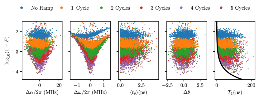
Figure 5: Performance of the SFQ pulse sequence as a function of the parameter variations for the 8$\times$ clock. We allow for deviations in the qubit anharmonicity $\alpha$, the frequency $\omega$, the jitter $\langle t_{\delta}\rangle$, and the kick angle $\theta$. We also include the effects of varying $T_{1}$, or, equivalently, the qubit decay rate $\gamma$.

To quantify the gate performance in the presence of leakage, timing jitter, and other possible errors, we use a more-general average gate fidelity metric [25]:

$$\overline{F}(\mathcal{E})=\frac{2F_{\textrm{pro}}(\mathcal{E})+1-L_{1}}{3},$$ (34)

where the process fidelity is defined as

$$F_{\textrm{pro}}(\mathcal{E})=\frac{1}{4}\Tr[S^{\dagger}_{G}(P_{2}\otimes P_{2})(S_{\mathcal{E}})],$$ (35)

where $P_{2}S_{\mathcal{E}}(P_{2})$ is the superoperator representation of the computed map projected onto the computational subspace, and $L_{1}=1-\Tr[P_{2}S_{\mathcal{E}}(P_{2})]/2$ quantifies the leakage of the channel.

For our simulations, we use a standard Lindbladian master equation:

$$\dot{\rho}=-i[\widehat{H}(t),\rho]+\gamma\mathcal{D}[\widehat{n}_{t}^{\Delta}]\rho\,,$$ (36)

where $\widehat{n}_{t}^{\Delta}$ is the upper-triangular matrix of the charge operator $\widehat{n}_{t}$. Translating this into the notation of SFQ kicks yields an effective evolution of the density matrix

$$\rho(t)=\left[\prod_{i}(\widehat{U}_{\textrm{kick}}\cdot\widehat{U}^{\dagger}_{\textrm{kick}})\exp(\mathcal{L}_{0}(t_{i}+t_{i,\delta}))\right]\rho(0),$$ (37)

where $\mathcal{L}_{0}=-i(\widehat{H}\cdot-\cdot\widehat{H})+\gamma\mathcal{D}[\widehat{n}_{t}^{\Delta}]\cdot$. Here, we include an additional error, the jitter time $t_{\delta,i}$. For each simulation, we suppose that the jitter time is sampled from a normal distribution with a standard deviation $\sigma=\langle t_{\delta}\rangle$, which is varied for each simulation. Further, we suppose that the kick angle $\theta$ is allowed to deviate by $\Delta\theta/1000$. The deviations in frequency and anharmonicity are centred around $\omega/2\pi=5$ GHz, $\alpha/2\pi=250$ MHz.

To test the robustness of the pulse train, we perform 1000 example simulations for each ramp length, with varying qubit parameters for the same chosen set of SFQ pulses. The results for the 8$\times$ clock are shown in Fig. 5.

Here, we restrict our focus to the $\widehat{R}_{Y}(\pi)$ gate, but have found similar results for other target angles. The samples are normally distributed around the parameters with which the gate is optimized.

We note that for the “no-ramp” evolution, the optimal frequency of the qubit is off-centre from the integer multiple of the clock. This is due to the phase shift induced by the virtual transitions to the leakage levels. As the number of ramps increases, the deviations become increasingly centred on the qubit frequency $(\Delta\omega=0)$, and the fidelity continues to improve.

Appendix B Spectral Components of the Pulse Sequences

To confirm that a given pulse sequence matches the behaviour of an equivalent DRAG pulse, we can analyze the spectrum of the pulse being delivered to the qubit. We begin by representing the pulse sequence for a 20 GHz external clock as a sum of Dirac delta functions,

$$f(t)=\sum_{m}\delta(t-mT/4),$$ (38)

where the indices $m$ are set by the number of pulses in the pulse train and the chosen ramp. We then take the Fourier transform, yielding

$$S(\omega)=\sum_{m}e^{2i\pi m\omega/4}.$$ (39)

In Fig. 6, we plot the spectrum Eq. 39 as a function of frequency for different ramp lengths, where the ramps are chosen so as to optimize the gate fidelity as described in Section V. As can be seen, the increasing length of the ramp steadily decreases the spectral intensity at the leakage frequency (indicated by the dashed line) as the ramp length increases. For four cycles, there is a reduction of more than an order of magnitude in the spectral component at this frequency, confirming that the SFQ ramps indeed reduce the spectral contribution at the leakage transition frequency. This method could be used to analyze possible ramps independently of unitary simulations, and thus identify candidates for high-fidelity ramps without the need to explore the entire search space.

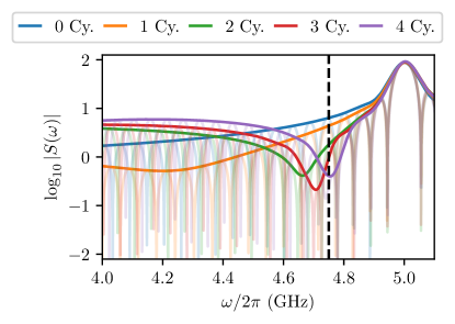
Figure 6: Fourier transform of a sequence of 87 pulses, beginning with no ramp (0 qubit cycles, shown in blue) and continuing up to a ramp of four qubit cycles (purple), optimized to implement an $\widehat{R}_{Y}(\pi)$ gate for the 20 GHz clock. The leakage frequency is indicated by a dashed line. The transparent lines indicate the true Fourier transform, while the opaque lines interpolate between each peak for clarity. As the number of ramps increases, the dip in spectral intensity is shifted with increasing accuracy to the leakage transition frequency.

References

- Blais et al. [2021] A. Blais, A. L. Grimsmo, S. M. Girvin, and A. Wallraff, Circuit quantum electrodynamics, Rev. Mod. Phys. 93, 025005 (2021).
- Kjaergaard et al. [2020] M. Kjaergaard, M. E. Schwartz, J. Braumüller, P. Krantz, J. I.-J. Wang, S. Gustavsson, and W. D. Oliver, Superconducting Qubits: Current State of Play, Annu. Rev. Condens. Matter Phys. 11, 369 (2020).
- Krinner et al. [2019] S. Krinner, S. Storz, P. Kurpiers, P. Magnard, J. Heinsoo, R. Keller, J. Lütolf, C. Eichler, and A. Wallraff, Engineering cryogenic setups for 100-qubit scale superconducting circuit systems, EPJ Quantum Technology 6, 2 (2019).
- McDermott and Vavilov [2014] R. McDermott and M. G. Vavilov, Accurate Qubit Control with Single Flux Quantum Pulses, Phys. Rev. Applied 2, 014007 (2014).
- McDermott et al. [2018] R. McDermott, M. G. Vavilov, B. L. T. Plourde, F. K. Wilhelm, P. J. Liebermann, O. A. Mukhanov, and T. A. Ohki, Quantum–classical interface based on single flux quantum digital logic, Quantum Sci. Technol. 3, 024004 (2018).
- Mancini and Bocko [1999] C. A. Mancini and M. F. Bocko, Phase-locked operation of RSFQ ring oscillators, Supercond. Sci. Technol. 12, 789 (1999).
- Lin and Semenov [1995] J.-C. Lin and V. Semenov, Timing circuits for RSFQ digital systems, IEEE Trans. Appl. Supercond. 5, 3472 (1995).
- Likharev and Semenov [1991] K. Likharev and V. Semenov, RSFQ logic/memory family: a new Josephson-junction technology for sub-terahertz-clock-frequency digital systems, IEEE Trans. Appl. Supercond. 1, 3 (1991).
- Nakajima et al. [1991] K. Nakajima, H. Mizusawa, H. Sugahara, and Y. Sawada, Phase mode Josephson computer system, IEEE Trans. Appl. Supercond. 1, 29 (1991).
- Leonard, Jr. et al. [2019] E. Leonard, Jr., M. A. Beck, J. Nelson, B. Christensen, T. Thorbeck, C. Howington, A. Opremcak, I. Pechenezhskiy, et al., Digital Coherent Control of a Superconducting Qubit, Phys. Rev. Applied 11, 014009 (2019).
- Howe et al. [2022] L. Howe, M. A. Castellanos-Beltran, A. J. Sirois, D. Olaya, J. Biesecker, P. D. Dresselhaus, S. P. Benz, and P. F. Hopkins, Digital Control of a Superconducting Qubit Using a Josephson Pulse Generator at 3 K, PRX Quantum 3, 010350 (2022).
- Liu et al. [2023] C. Liu, A. Ballard, D. Olaya, D. Schmidt, J. Biesecker, T. Lucas, J. Ullom, S. Patel, et al., Single Flux Quantum-Based Digital Control of Superconducting Qubits in a Multichip Module, PRX Quantum 4, 030310 (2023).
- Liebermann and Wilhelm [2016] P. J. Liebermann and F. K. Wilhelm, Optimal Qubit Control Using Single-Flux Quantum Pulses, Phys. Rev. Applied 6, 024022 (2016).
- Vogt and Petersson [2022] R. H. Vogt and N. A. Petersson, Binary Optimal Control of Single-Flux-Quantum Pulse Sequences, SIAM J. Control Optim. 60, 3217 (2022).
- Mukhanov [1993] O. Mukhanov, Rapid single flux quantum (RSFQ) shift register family, IEEE Trans. Appl. Supercond. 3, 2578 (1993).
- Li et al. [2019] K. Li, R. McDermott, and M. G. Vavilov, Hardware-Efficient Qubit Control with Single-Flux-Quantum Pulse Sequences, Phys. Rev. Applied 12, 014044 (2019).
- Krinner et al. [2022] S. Krinner, N. Lacroix, A. Remm, A. Di Paolo, E. Genois, C. Leroux, C. Hellings, S. Lazar, et al., Realizing repeated quantum error correction in a distance-three surface code, Nature 605, 669 (2022).
- Google Quantum AI [2023] Google Quantum AI, Suppressing quantum errors by scaling a surface code logical qubit, Nature 614, 676 (2023).
- Khaneja et al. [2005] N. Khaneja, T. Reiss, C. Kehlet, T. Schulte-Herbrüggen, and S. J. Glaser, Optimal control of coupled spin dynamics: design of NMR pulse sequences by gradient ascent algorithms, J. Magn. Reson. 172, 296 (2005).
- Motzoi et al. [2009] F. Motzoi, J. M. Gambetta, P. Rebentrost, and F. K. Wilhelm, Simple Pulses for Elimination of Leakage in Weakly Nonlinear Qubits, Phys. Rev. Lett. 103, 110501 (2009).
- Koch et al. [2007] J. Koch, T. M. Yu, J. Gambetta, A. A. Houck, D. I. Schuster, J. Majer, A. Blais, M. H. Devoret, et al., Charge-insensitive qubit design derived from the Cooper pair box, Phys. Rev. A 76, 042319 (2007).
- Motzoi and Wilhelm [2013] F. Motzoi and F. K. Wilhelm, Improving frequency selection of driven pulses using derivative-based transition suppression, Phys. Rev. A 88, 062318 (2013).
- Lucero et al. [2010] E. Lucero, J. Kelly, R. C. Bialczak, M. Lenander, M. Mariantoni, M. Neeley, A. D. O’Connell, D. Sank, et al., Reduced phase error through optimized control of a superconducting qubit, Phys. Rev. A 82, 042339 (2010).
- McKay et al. [2017] D. C. McKay, C. J. Wood, S. Sheldon, J. M. Chow, and J. M. Gambetta, Efficient gates for quantum computing, Phys. Rev. A 96, 022330 (2017).
- Wood and Gambetta [2018] C. J. Wood and J. M. Gambetta, Quantification and characterization of leakage errors, Phys. Rev. A 97, 032306 (2018).
- Yamanashi et al. [2021] Y. Yamanashi, R. Kinoshita, and N. Yoshikawa, Frequency synchronization of single flux quantum oscillators, Supercond. Sci. Technol. 34, 105004 (2021).
- Chen et al. [1998] W. Chen, A. V. Rylyakov, V. Patel, J. E. Lukens, and K. K. Likharev, Superconductor digital frequency divider operating up to 750 GHz, Appl. Phys. Lett. 73, 2817 (1998).
- Jokar et al. [2021] M. R. Jokar, R. Rines, and F. T. Chong, Practical implications of SFQ-based two-qubit gates, in 2021 IEEE International Conference on Quantum Computing and Engineering (QCE) (2021) pp. 402–412.
- Caldwell et al. [2018] S. A. Caldwell, N. Didier, C. A. Ryan, E. A. Sete, A. Hudson, P. Karalekas, R. Manenti, M. P. da Silva, et al., Parametrically Activated Entangling Gates Using Transmon Qubits, Phys. Rev. Appl. 10, 034050 (2018).
- Moskalenko et al. [2022] I. N. Moskalenko, I. A. Simakov, N. N. Abramov, A. A. Grigorev, D. O. Moskalev, A. A. Pishchimova, N. S. Smirnov, V. Zikiy, Evgeniy, et al., High fidelity two-qubit gates on fluxoniums using a tunable coupler, npj Quantum Inf. 8, 130 (2022).