Motif-aware Attribute Masking for
Molecular Graph Pre-training

Abstract

Attribute reconstruction is used to predict node or edge features in the pre-training of graph neural networks. Given a large number of molecules, they learn to capture structural knowledge, which is transferable for various downstream property prediction tasks and vital in chemistry, biomedicine, and material science. Previous strategies that randomly select nodes to do attribute masking leverage the information of local neighbors However, the over-reliance of these neighbors inhibits the model’s ability to learn from higher-level substructures. For example, the model would learn little from predicting three carbon atoms in a benzene ring based on the other three but could learn more from the inter-connections between the functional groups, or called chemical motifs. In this work, we propose and investigate motif-aware attribute masking strategies to capture inter-motif structures by leveraging the information of atoms in neighboring motifs. Once each graph is decomposed into disjoint motifs, the features for every node within a sample motif are masked. The graph decoder then predicts the masked features of each node within the motif for reconstruction. We evaluate our approach on eight molecular property prediction datasets and demonstrate its advantages.

1 Introduction

Molecular property prediction has been an important topic of study in fields such as physical chemistry, physiology, and biophysics [1]. It can be defined as a graph label prediction problem and addressed by machine learning. However, the graph learning models such as graph neural networks (GNNs) must overcome issues in data scarcity, as the creation and testing of real-world molecules is an expensive endeavor [2]. To address labeled data scarcity, model pre-training has been utilized as a fruitful strategy for improving a model’s predictive performance on downstream tasks, as pre-training allows for the transfer of knowledge from large amounts of unlabeled data. The selection of pre-training strategy is still an open question, with contrastive tasks [3] and predictive/generative tasks [4] being the most popular methods.

Attribute reconstruction is one predictive method for graphs that utilizes masked autoencoders to predict node or edge features [4, 5, 6]. Masked autoencoders have found success in vision and language domains [7, 8] and have been adopted as a pre-training objective for graphs as the reconstruction task is able to transfer structural pattern knowledge [4], which is vital for learning specific domain knowledge such as valency in material science. Additional domain knowledge which is important for molecular property prediction is that of functional groups, also called chemical motifs [9]. The presence and interactions between chemical motifs directly influence molecular properties, such as reactivity and solubility [10, 11]. Therefore, to capture the interaction information between motifs, it is important to transfer inter-motif structural knowledge during the pre-training of graph neural networks.

Unfortunately, the random attribute masking strategies used in previous work for graph pre-training were not able to capture the inter-motif structural knowledge [5, 12, 13]. That is because they rely on neighboring node feature information for reconstruction  [4, 14]. Notably, leveraging the features of local neighbors can contribute to learning important local information, including valency and atomic bonding. However, GNNs heavily rely on the neighboring node’s features rather than graph structure [15], and this over-reliance inhibits the model’s ability to learn from motif structures as message aggregation will prioritize local node feature information due to the propagation bottleneck [16]. For example, as shown on the left-hand side of Figure 1, if only a (small) partial set of nodes were masked in several motifs, the pre-trained GNNs would learn to predict the node types (i.e., carbon) of two atoms in the benzene ring based on the node features of the other four carbon atoms in the ring.

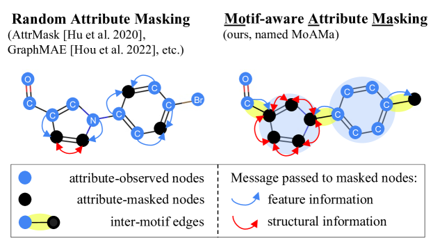
Figure 1: Our MoAMa masks every node in a motif to pre-train GNNs. The full masking of a motif forces the GNNs to learn to (1) pass feature information across motifs and (2) pass local structural information within the motif. Compared to the traditional random attribute masking strategies, the motif-aware masking captures the most essential information to learn graph embeddings. Random masking would put most of the pre-training effort on passing the feature information within a motif, e.g., predicting two carbon nodes in a benzene ring based on the other four.

Because a random masking strategy is not guaranteed to transfer inter-motif structural knowledge into downstream, we propose a novel masking strategy that forces the transfer of inter-motif knowledge. In Figure 1, we visually demonstrate our method for motif-aware attribute masking, where for each molecular graph, we decompose it into disjoint motifs. Then the node features for each node within the motif will be masked by a mask token. A graph decoder will predict the masked features of each node within the motif as the reconstruction task. The benefits of this strategy are twofold. First, because all features of the nodes within the motif are masked, our strategy reduces the amount of feature information being passed within the motif and relieves the propagation bottleneck, allowing for the greater transfer of inter-motif feature and structural information. Second, the masking of all intra-motif node features explicitly forces the decoder to transfer intra-motif structural information. A novel graph pre-training solution based on the Motif-aware Attribute Masking strategy, called MoAMa , is able to utilize the intra-motif structural information while being able to utilize the inter-motif features. We evaluate our strategy on eight molecular property prediction datasets and demonstrate its strength against previous strategies.

The main contributions of this work are summarized as follows:

• We propose a novel effective motif-aware graph pre-training strategy for molecular property prediction tasks to overcome the limitations of existing random attribute masking methods.

• We design, develop, and evaluate a graph pre-training solution MoAMa based on the new strategy. We investigate the effect of various configurations of the strategy and solution.

• Experiments demonstrate MoAMa’s competitive performance with state-of-the-art methods, improving predictive accuracy on average by 1.3%, as compared to the best baseline.

2 Related Work

Molecular graph pre-training

The prediction of molecular properties based on graphs is important [1]. Molecules are scientific data that are time- and computation-intensive to collect and annotate for different property prediction tasks [17]. Many self-supervised learning methods [4, 14, 18, 19, 20] were proposed to capture the transferable knowledge from another large scale of molecules without annotations. For example, AttrMask [4] randomly masked atom attributes for prediction. GraphMAE [14] pre-trained the prediction model with generative tasks to reconstruct node and edge attributes. D-SLA [19] used contrastive learning based on graph edit distance. These pre-training tasks could not well capture useful knowledge for various domain-specific tasks since they fail to incorporate important domain knowledge in pre-training. A great line of prior work [18, 21, 22] used graph motifs which are the recurrent and statistically significant subgraphs to characterize the domain knowledge contained in molecular graph structures, e.g., functional groups. However, their solutions were tailored to specific frameworks for either generation-based or contrast-based molecular pre-training. Additionally, explicit motif type generation/prediction inherently does not transfer intra-motif structural information and is computationally expensive due to the large number of prediction classes. In this work, we study on the strategies of attribute masking with the awareness of domain knowledge (i.e., motifs), which plays an essential role in self-supervised learning frameworks [20].

Masking strategies on molecules

Attribute masking of atom nodes is a popular method in graph pre-training given its broad usage in predictive, generative, and contrastive self-supervised tasks [4, 12, 14, 23, 24]. For example, predictive and generative pre-training tasks [4, 14, 20] mask atom attributes for prediction and reconstruction. Contrastive pre-training tasks [23, 24] mask nodes to create another data view for alignment. Despite the widespread use of attribute masking in molecular pre-training, there is a notable absence of comprehensive research on its strategy and effectiveness. Previous studies have largely adopted strategies from the vision and language domains [7, 8], where atom attributes are randomly masked with a predetermined ratio. Since molecules are atoms held together by strict chemical rules, the data modality of molecular graphs is essentially different from natural images and languages. For molecular graphs, random attribute masking results in either over-reliance on intra-motif neighbors or breaking the inter-motif connections. In this work, we introduce a novel strategy of attribute masking, which turns out to capture and transfer useful knowledge from intra-motif structures and inter-motif node features.

3 Preliminaries

Graph property prediction

Given a graph $G=(\mathcal{V},\mathcal{E})\in\mathcal{G}$ with the node set $\mathcal{V}$ for atoms and the edge set $\mathcal{E}\subset\mathcal{V}\times\mathcal{V}$ for bonds, we have a $d$-dimensional node attribute matrix $\mathbf{X}\in\mathbb{R}^{|\mathcal{V}|\times d}$ that represents atom features such as atom type and chirality. We use $y\in\mathcal{Y}$ as the graph-level property label for $G$, where $\mathcal{Y}$ represents the label space. For graph property prediction, a predictor with the encoder-decoder architecture is trained to encode $G$ into a representation vector in the latent space and decode the representation to predict $\hat{y}$. The training process optimizes the parameters to make $\hat{y}$ to be the same as the true label value $y$. Usually, we use a GNN as the encoder. It generates $k$-dimensional node representation vectors, denoted as $\mathbf{h}_{v}\in\mathbb{R}^{k}$, for any node $v\in\mathcal{V}$:

$$\mathbf{H}=\{\mathbf{h}_{v}:v\in\mathcal{V}\}=\operatorname{GNN}(G)\in\mathbb{R}^{|\mathcal{V}|\times k}.$$ (1)

Here $\mathbf{H}$ is the node representation matrix for the graph $G$. Without loss of generality, we follow previous work [4] to implement the GNN with Graph Isomorphism Networks (GIN) [25]. Once we have the set of node representations, we use a $\operatorname{READOUT}(\cdot$) function (such as max, mean, or sum) to summarize the node-level representation into graph-level representation $\mathbf{h}_{G}$ for any $G$:

$$\mathbf{h}_{G}=\operatorname{READOUT}(\mathbf{H})\in\mathbb{R}^{k}.$$ (2)

We pass the node representation matrix $\mathbf{H}$ into the $\operatorname{READOUT}(\cdot$) function to create the graph-level representation vector $\mathbf{h}_{G}$. Then, $\mathbf{h}_{G}$ is passed through a multi-layer perceptron (MLP) to generate the label prediction $\hat{y}$ which exists in the label space $\mathcal{Y}$:

$$\hat{y}=\operatorname{MLP}(\mathbf{h}_{G})\in\mathcal{Y}.$$ (3)

GNN pre-training

Random initialization of the predictor’s parameters would easily result in suboptimal solutions for graph property prediction. This is because the number of labeled graphs is usually small. It prevents a proper coverage of task-specific graph and label space [4, 17]. To improve generalization, GNN pre-training is often used to warm-up the model parameters based on a much larger set of molecules without labels. In this work, we focus on the attribute masking strategy for GNN pre-training that aims to predict the masked values of node attributes given the unlabeled graphs.

4 Proposed Solution

In this section, we present our novel solution named MoAMa for effectively pre-training graph neural networks on molecular data. We will give details about the strategy of motif-aware attribute masking and reconstruction. Each molecule $G$ will have some portion of their node masked according to domain knowledge based motifs. We replace the node attributes of all masked nodes with a special mask token. Then, the $\operatorname{GNN}$ in Eq. (1) encodes the masked graph to the node representation space, and an $\operatorname{MLP}$ reconstructs the atom types for the attribute masked molecule.

4.1 Knowledge-based Motif Extraction

To leverage the expertise from the chemistry domain, we first extract motifs for molecules. We achieve this using the BRICS (Breaking of Retrosynthetically Interesting Chemical Substructures) algorithm [26]. This algorithm leverages chemical domain knowledge by creating 16 rules for decomposition, the rules of which define the bonds that should be cleaved from the molecule in order to create a multi-set of disjoint subgraphs. Two key strengths of the BRICS algorithm over a motif-mining strategy [27] is that no training is required and important structural features, such as rings, are inherently preserved.

For each graph $G$, we use the BRICS algorithm to decompose it into separate motifs. We denote the decomposition result as $\mathcal{M}_{G}=\{M_{1},M_{2},...,M_{n}\}$, which is a set of $n$ motifs. Each motif $M_{i}=(\mathcal{V}_{i},\mathcal{E}_{i})$, for $i\in\{1,2,...,n\}$, is a disjoint subgraph of $G$ such that $\mathcal{V}_{i}\subset\mathcal{V}$ and $\mathcal{E}_{i}\subset\mathcal{E}$. For each motif multi-set $\mathcal{M}_{G}$, the union of all motifs $M_{i}\in\mathcal{M}_{G}$ should equal $G$. Formally, this means $\mathcal{V}=\bigcup_{i}V_{i}$ and $\mathcal{E}=\left(\bigcup_{i}E_{i}\right)\bigcup E_{x}$, where $E_{x}$ represents all the edges removed between motifs during the BRICS decomposition. Within the ZINC15 dataset [28], each molecule has an average of 9.8 motifs, each of which have an average of 2.4 atoms.

4.2 Motif-aware Attribute Masking and Reconstruction

To perform motif-aware attribute masking, we first sample $m$ motifs to form the multi-set $\mathcal{M}_{G}^{\prime}\subset\mathcal{M}_{G}$ such that $(\sum_{(\mathcal{V}_{i},\mathcal{E}_{i})\in\mathcal{M}_{G}^{\prime}}|\mathcal{V}_{i}|)/|\mathcal{V}|=\alpha$. The motifs sampled for $\mathcal{M}_{G}^{\prime}$ must adhere to two criteria: (1) each node within the motif must be within a $k$-hop neighborhood ($k$ equals number of GNN layers) of an inter-motif node, and (2) sampled motifs may not be adjacent. These two criteria guarantee inter-motif knowledge access for each masked node. To adhere to the above criteria and account for variable motif sizes, we allow for some flexibility in the value for $\alpha$. We choose the bounds $0.15<\alpha<0.25$ in accordance to those used in previous works ($\alpha=0.15$ [4] and $\alpha=0.25$ [14]).

Given a selected motif $M\in\mathcal{M}^{\prime}_{G}$, nodes within $M$ have their attributes masked by replacing them with a mask token [MASK], which is a vector $\mathbf{m}\in\mathbb{R}^{d}$. Each element in $\mathbf{m}$ is a special value that is not present within the attribute space for that particular dimension. For example, we may set the attribute for the atom type dimension in $\mathbf{m}$ to the value $119$, as we totally have $118$ atom types [4]. We use $\mathcal{V}_{\text{[MASK]}}=\{v\in\mathcal{V}_{i}:M_{i}=(\mathcal{V}_{i},\mathcal{E}_{i})\in\mathcal{M}_{G}^{\prime}\}$ to denote the set of all the masked nodes. Then we could define the input node features as the masked attribute matrix $\mathbf{X}_{\text{[MASK]}}\in\mathbb{R}^{|\mathcal{V}|\times d}$ by defining any $v\in\mathcal{V}$ in it as follows:

$${(\mathbf{X}_{\text{[MASK]}})}_{v}=\begin{cases}\mathbf{X}_{v},&v\notin\mathcal{V}_{\text{[MASK]}},\\ \mathbf{m},&v\in\mathcal{V}_{\text{[MASK]}},\end{cases}$$ (4)

where ${(\mathbf{X}_{\text{[MASK]}})}_{v}$ and $\mathbf{X}_{v}$ denote the row of the node $v$ in $\mathbf{X}_{\text{[MASK]}}$ and $\mathbf{X}$, respectively. With a $\operatorname{GNN}$ encoder, all nodes with attributes $\mathbf{X}_{\text{[MASK]}}$ for the masked graph $G_{\text{[MASK]}}$ are encoded to the latent representation space according to Eq.(1): $\mathbf{H}=\operatorname{GNN}(G_{\text{[MASK]}})$. Then we define the reconstruction loss of the node attributes as:

$$\mathcal{L}_{\text{rec}}=\mathbb{E}_{v\in\mathcal{V}_{\text{[MASK]}}}[\log p(\mathbf{X}|\mathbf{H})],$$ (5)

where $p(\mathbf{X}|\mathbf{H})$ for the reconstruction attribute value is inferred by a decoder.

We use scale cosine error (SCE) [14] to measure the difference between the probability distribution for the reconstruction attributes and the one-hot encoded target label vector.

4.3 Design Space of the Attribute Masking Strategy

The design space of the motif-aware node attribute masking includes four parts as follows.

Masking distribution

We first investigate the influence of masking distribution to the masking strategy. We use two factors to control the distribution of masked attributes:

• Percentage of nodes within a motif selected for masking: we propose to mask nodes from the selected motifs at different percentages. The percentage indicates the strength of the masked domain knowledge, which affects the hardness of the pre-training task of the attribute reconstruction.

• Dimension of the attributes: We propose to conduct either node-wise or element-wise (dimension-wise) masking. Element-wise masking selects different nodes for masking in different dimensions according to the percentage, while node-wise masking selects different nodes for all-dimensional attribute masking in different motifs.

Reconstruction target

Existing molecular graph pre-training methods heavily rely on two atom attributes: atom type and chirality. Therefore, we could reconstruct one of them or both of them with one or two different decoders. Experiments will find the most effective task definition.

Reconstruction loss

We study different implementations of reconstruction loss functions for $\mathcal{L}_{\text{rec}}$. They include cross entropy (CE), scaled cosine error (SCE) [14], and mean square error (MSE). GraphMAE [14] suggested that SCE was the best loss function, however, it is worth investigating the effect of the loss function choices in the motif-based study.

Additionally, attribute masking focuses on local graph structures and suffers from representation collapse [4, 14]. To address this issue, we use a knowledge-enhanced auxiliary loss $\mathcal{L}_{\text{aux}}$ to complement $\mathcal{L}_{\text{rec}}$. Given any two graphs $G_{i}$ and $G_{j}$ from the graph-based chemical space $\mathcal{G}$, $\mathcal{L}_{\text{aux}}$ first calculates the Tanimoto similarity [29] between $G_{i}$ and $G_{j}$ as $\operatorname{Tanimoto}(G_{i},G_{j})$ based on the bit-wise fingerprints, which characterizes frequent fragments in the molecular graphs. Then $\mathcal{L}_{\text{aux}}$ aligns the latent representations with the Tanimoto similarity using the $\operatorname{cosine}$ similarity. Formally, we define:

$$\mathcal{L}_{\text{aux}}=\sum_{i,j}\left(\operatorname{Tanimoto}(G_{i},G_{j})-\operatorname{cosine}(\mathbf{h}_{G_{i}},\mathbf{h}_{G_{j}})\right),1\leq i,j\leq|\mathcal{G}|,i\not=j,$$ (6)

where $\mathbf{h}_{G_{i}}$ and $\mathbf{h}_{G_{j}}$ are the graph representation of $G_{i}$ and $G_{j}$, respectively.

The full pre-training loss is $\mathcal{L}=\beta\mathcal{L}_{\text{rec}}+(1-\beta)\mathcal{L}_{\text{aux}}$, where $\beta$ is a hyperparameter to balance these two loss terms.

Decoder model

Finally, we research the effect of the decoder models. The decoder trained via Eq. (5) could be a $\operatorname{GNN}$ or a $\operatorname{MLP}$. Although the $\operatorname{GNN}$ decoder might be powerful [14], we are curious if the $\operatorname{MLP}$ delivers a comparable or better performance with higher efficiency.

5 Experiments

5.1 Experimental Settings

Table 1: Test AUC (%) performance on eight molecular datasets comparing our method with baselines. The best AUC-ROC values for each dataset are in bold.

	MUV	ClinTox	SIDER	HIV	Tox21	BACE	ToxCast	BBBP	Avg
No Pretrain	70.7$\pm$1.8	58.4$\pm$6.4	58.2$\pm$1.7	75.5$\pm$0.8	74.6$\pm$0.4	72.4$\pm$3.8	61.7$\pm$0.5	65.7$\pm$3.3	67.2
MCM [30]	74.4$\pm$0.6	64.7$\pm$0.5	62.3$\pm$0.9	72.7$\pm$0.3	74.4$\pm$0.1	79.5$\pm$1.3	61.0$\pm$0.4	71.6$\pm$0.6	69.7
MGSSL [18]	77.6$\pm$0.4	77.1$\pm$4.5	61.6$\pm$1.0	75.8$\pm$0.4	75.2$\pm$0.6	78.8$\pm$0.9	63.3$\pm$0.5	68.8$\pm$0.9	72.3
Grover [21]	50.6$\pm$0.4	75.4$\pm$8.6	57.1$\pm$1.6	67.1$\pm$0.3	76.3$\pm$0.6	79.5$\pm$1.1	63.4$\pm$0.6	68.0$\pm$1.5	67.2
AttrMask [4]	75.8 $\pm$1.0	73.5$\pm$4.3	60.5$\pm$0.9	75.3$\pm$1.5	75.1$\pm$0.9	77.8$\pm$1.8	63.3$\pm$0.6	65.2$\pm$1.4	70.8
ContextPred [4]	72.5$\pm$1.5	74.0$\pm$3.4	59.7$\pm$1.8	75.6$\pm$1.0	73.6$\pm$0.3	78.8$\pm$1.2	62.6$\pm$0.6	70.6$\pm$1.5	70.9
GraphMAE [14]	76.3$\pm$2.4	82.3$\pm$1.2	60.3$\pm$1.1	77.2$\pm$1.0	75.5$\pm$0.6	83.1$\pm$0.9	64.1$\pm$0.3	72.0$\pm$0.6	73.9
Mole-BERT [20]	78.6$\pm$1.8	78.9$\pm$3.0	62.8$\pm$1.1	78.2$\pm$0.8	76.8$\pm$0.5	80.8$\pm$1.4	64.3$\pm$0.2	71.9$\pm$1.6	74.0
JOAO [24]	76.9$\pm$0.7	66.6$\pm$3.1	60.4$\pm$1.5	76.9$\pm$0.7	74.8$\pm$0.6	73.2$\pm$1.6	62.8$\pm$0.7	66.4$\pm$1.0	71.1
GraphLoG [31]	76.0$\pm$1.1	76.7$\pm$3.3	61.2$\pm$1.1	77.8$\pm$0.8	75.7$\pm$0.5	83.5$\pm$1.2	63.5$\pm$0.7	72.5$\pm$0.8	73.4
D-SLA [19]	76.6$\pm$0.9	80.2$\pm$1.5	60.2$\pm$1.1	78.6$\pm$0.4	76.8$\pm$0.5	83.8$\pm$1.0	64.2$\pm$0.5	72.6$\pm$0.8	73.9
MoAMa w/o $\mathcal{L}_{\text{aux}}$	78.5$\pm$0.4	84.2$\pm$0.8	61.2$\pm$0.2	79.5$\pm$0.5	76.2$\pm$0.3	84.1$\pm$0.2	64.6$\pm$0.1	71.8$\pm$0.7	75.0
MoAMa	80.0$\pm$0.8	85.3$\pm$2.2	64.6$\pm$0.5	79.3$\pm$0.6	76.5$\pm$0.1	80.1$\pm$0.5	63.0$\pm$0.4	72.8$\pm$0.9	75.3

Datasets

To pre-train GNN models, we use 2 million unlabeled molecules from the ZINC15 dataset [28] following the setting of previous studies [14, 19, 20]. To evaluate the performance on downstream tasks, we conduct experiments across eight binary classification benchmark datasets from MoleculeNet [1].

Validation methods and evaluation metrics

In accordance with previous work, we adopt a scaffold splitting approach [4, 18]. Random splitting may not reflect the actual use case, so molecules are divided according to structures into train, validation, and test sets [1], using a 80:10:10 split for the three sets. We use the area under the ROC curve (AUC) to evaluate the performance of the classification models during 10 independent runs.

Model configurations

For fair comparison with previous work, we utilize a five-layer Graph Isomorphism Network (GIN) as our GNN encoder. The embedding dimension for the GIN is 300. The $\operatorname{READOUT}$ strategy for the graph representation is mean pooling. During pre-training and finetuning, we train our models for 100 epochs using a learning rate of 0.001 using the Adam optimizer. The batch size for pre-training and finetuning is 256 and 32 respectively.

5.2 Baselines

There are two general types of baseline graph pre-training strategies that we evaluate our work against, those involving contrastive learning tasks, such as D-SLA [19], GraphLoG [31], and JOAO [24], and those involving attribute reconstruction, including Grover [21], AttrMask [4], ContextPred [4], GraphMAE [14], and Mole-BERT [20]. Additionally, we evaluate on motif-based pre-training strategies, MGSSL [18], which recurrently generates the motif tree for any molecule, and MCM [30], which uses a motif-based convolution module to generate embeddings.

5.3 Results

We report AUC-ROC of different graph pre-training methods in Table 1. MoAMa outperforms all previous methods on five out of eight datasets. On average, MoAMa outperforms the best baseline method Mole-BERT [20] by $1.3\%$ and the best contrastive learning methods D-SLA [19] by $1.4\%$. Even without the auxiliary loss $\mathcal{L}_{\text{aux}}$, our motif-aware masking strategy still maintains a performance improvement of $1.0\%$, which is still competitive with previous methods.

5.4 Ablation Studies

To verify motif-aware masking parameters, we conduct ablation studies on the selection of masking distributions, reconstruction target attribute(s), reconstruction loss function, and decoder model.

Table 2: Strategy design for motif-aware attribute masking: (1) masking distribution, (2) reconstruction target, (3) reconstruction loss, and (4) decoder model. The chosen design is highlighted.

Design Space		MUV	ClinTox	SIDER	HIV	Tox21	BACE	ToxCast	BBBP	Avg
(1)	100% Motif Coverage	80.0$\pm$0.8	85.3$\pm$2.2	64.6$\pm$0.5	79.3$\pm$0.6	76.5$\pm$0.1	80.1$\pm$0.5	63.0$\pm$0.4	72.8$\pm$0.9	75.3
	75% Node-wise	74.9$\pm$1.1	82.3$\pm$0.4	60.1$\pm$0.3	78.8$\pm$0.9	76.1$\pm$0.1	82.3$\pm$0.4	63.4$\pm$0.1	72.1$\pm$1.0	73.7
	75% Element-wise	74.8$\pm$0.7	84.9$\pm$1.0	58.7$\pm$0.1	79.7$\pm$0.7	75.6$\pm$0.1	85.7$\pm$0.4	63.4$\pm$0.2	72.6$\pm$0.4	74.4
	50% Node-wise	76.6$\pm$1.2	86.4$\pm$0.6	58.3$\pm$0.1	78.1$\pm$0.3	75.1$\pm$0.2	81.9$\pm$0.3	64.6$\pm$0.1	72.7$\pm$0.1	74.2
	50% Element-wise	73.9$\pm$0.2	71.2$\pm$4.0	61.2$\pm$0.4	77.5$\pm$0.8	74.9$\pm$0.4	81.1$\pm$0.7	62.5$\pm$0.1	70.6$\pm$1.8	71.6
	25% Node-wise	76.6$\pm$1.5	86.3$\pm$0.7	62.4$\pm$0.2	78.4$\pm$0.2	75.9$\pm$0.2	81.8$\pm$0.1	65.1$\pm$0.1	74.7$\pm$0.2	75.1
	25% Element-wise	75.2$\pm$1.5	82.1$\pm$0.4	58.3$\pm$0.1	77.8$\pm$1.5	75.5$\pm$0.2	81.5$\pm$0.2	63.1$\pm$0.1	71.6$\pm$0.3	73.1
(2)	Atom Type	80.0$\pm$0.8	85.3$\pm$2.2	64.6$\pm$0.5	79.3$\pm$0.6	76.5$\pm$0.1	80.1$\pm$0.5	63.0$\pm$0.4	72.8$\pm$0.9	75.3
	Chirality	76.3$\pm$1.8	75.1$\pm$0.9	59.8$\pm$0.5	77.9$\pm$0.1	76.6$\pm$0.1	79.8$\pm$0.5	63.8$\pm$0.2	73.8$\pm$0.7	72.9
	Both w/ one decoder	76.2$\pm$1.4	74.4$\pm$1.1	62.4$\pm$0.9	78.2$\pm$1.1	75.5$\pm$0.6	82.1$\pm$0.4	64.3$\pm$0.2	72.9$\pm$0.2	73.3
	Both w/ two decoders	75.9$\pm$0.9	81.5$\pm$0.1	60.5$\pm$0.1	78.5$\pm$0.9	75.8$\pm$0.2	82.0$\pm$1.0	63.7$\pm$0.3	73.4$\pm$0.3	73.9
(3)	Scaled Cosine Error	80.0$\pm$0.8	85.3$\pm$2.2	64.6$\pm$0.5	79.3$\pm$0.6	76.5$\pm$0.1	80.1$\pm$0.5	63.0$\pm$0.4	72.8$\pm$0.9	75.3
	Cross Entropy	78.8$\pm$1.1	84.5$\pm$0.7	65.4$\pm$0.2	78.6$\pm$0.4	76.3$\pm$0.1	82.4$\pm$0.2	62.9$\pm$0.5	72.3$\pm$0.2	75.1
	Mean Squared Error	80.0$\pm$0.5	84.1$\pm$1.4	64.6$\pm$0.5	78.3$\pm$0.4	76.8$\pm$0.2	80.5$\pm$0.6	62.8$\pm$0.3	71.8$\pm$0.6	74.9
(4)	GNN decoder	80.0$\pm$0.8	85.3$\pm$2.2	64.6$\pm$0.5	79.3$\pm$0.6	76.5$\pm$0.1	80.1$\pm$0.5	63.0$\pm$0.4	72.8$\pm$0.9	75.3
	MLP decoder	78.8$\pm$0.5	85.2$\pm$0.1	65.5$\pm$0.3	78.1$\pm$0.6	76.2$\pm$0.2	82.1$\pm$0.6	62.8$\pm$0.8	71.7$\pm$0.4	75.1

5.4.1 Study on Masking Distributions

For motif-aware masking, we have the choice of masking the features of all nodes within the motif or choosing to only mask the features of a percentage of nodes within each sampled motif. For our study, we choose a motif coverage parameter to decide what percentage of nodes within each motif to mask, ranging from $25\%$, $50\%$, $75\%$, or $100\%$.

Furthermore, the masking strategy utilized by previous work performs node-wise masking [4, 14], where all features of a node are masked. An alternative strategy may be element-wise masking, where masked elements are chosen over all feature dimensions. This means that not all features of a node may necessarily be masked. The mask percentage parameter controls how many total features will be masked. For example, if the mask percentage parameter is 25%, then 25% of nodes within a sampled motif will have their atom types masked and 25% of nodes will have their chirality masked. The nodes within each mask set may be disjoint or completely overlap. Note that 100% masking will behave the exact same as node-wise masking, as 100% of nodes within a motif will have each feature masked.

We provide the predictive performance within Table 2. The predictive performance for the node-wise masking outperforms the element-wise masking for both 25% and 50% node coverage. At 75% coverage, element-wise masking outperforms node-wise. However, the full coverage masking strategy outperforms all other masking strategies.

5.4.2 Study on Reconstruction Targets

The choice of attributes to reconstruct for GNNs towards molecular property prediction has traditionally been atom type [4, 14]. However, there are other choices for reconstruction that could be explored. We verify the choice of reconstruction attrbutes by comparing the performance of the baseline model against models trained by reconstructing only chirality, both atom type and chirality using one unified decoder, or both atom type and chirality using two separate decoders. From Table 2, we note that predicting solely atom type yields the best pre-training results. The second best strategy was to predict both atom type and chirality using two decoders. In this case, the loss of the two decoders are independent, leading to the conclusion that the chirality prediction task is ill-suited to be the pre-training task. Because choice of chirality is limited to four extremely imbalanced outputs, the transferable knowledge may be significantly lesser than that of atom prediction which, for the ZINC15 dataset, has nine types.

5.4.3 Study on Reconstruction Loss Functions

For the pretraining task, we have three choices of error functions to calculate training loss. A standard error function used for masked autoencoders within computer vision [7, 32, 33] is the cross-entropy loss, whereas previous GNN solutions utilize mean squared error (MSE) [12, 34, 35, 36]. GraphMAE [14] proposed that cosine error could mitigate sensitivity and selectivity issues:

$$\mathcal{L}_{\text{rec}}=\frac{1}{|\mathcal{V}_{\text{[MASK]}}|}\sum_{v\in\mathcal{V}_{\text{[MASK]}}}(1-\frac{\mathbf{X}_{v}^{T}\mathbf{H}_{v}}{||\mathbf{X}_{v}||\cdot||\mathbf{H}_{v}||})^{\gamma},\gamma\geq 1.$$ (7)

This equation is called the scaled cosine error (SCE). $\mathbf{H}$ are the reconstructed features, $\mathbf{X}$ are the ground-truth node features, and $\gamma$ is a scaling factor. For our tests, we kept this value at $1$, following the setting of the previous work.

We investigate the effect these different error functions have on downstream predictive performance in Table 2. In accordance with previous work, we find SCE outperforms CE and MSE.

5.4.4 Study on Decoder Model Choices

We follow the GNN decoder settings from previous work [14] to conduct our study to determine which decoder leads to better downstream predictive performance. In Table 2, we show that our method outperforms the MLP-decoder strategy, which support previous work that show MLP-based decoders lead to reduced model expressiveness of the inability of MLPs to utilize the high number of embedded features [14].

5.5 Inter-motif Influence Analysis

A traditional assumption was that a node would receive stronger influence from intra-motif nodes than from inter-motif nodes, due to shorter distance on the graph. While we have observed the accuracy advantages of motif-aware masking, we are curious about whether the assumption was broken by this novel strategy – the inter-motif influence may play a significant role in predicting node attributes and molecular graph pre-training.

To measure the influence generally from (either intra-motif or inter-motif) source nodes on a target node $v$, we must design a measure that quantifies the influence from any source node $u$ in the same graph $G$, denoted by $s(u,v)$. $\mathbf{h}_{v}$ was learned by Eq. (1) and was influenced by node $u$. If we eliminated the embedding of $u$ since GNN initialization, i.e., set $\mathbf{h}_{u}^{(0)}=\vec{0}$, Eq. (1) would give us a new representation vector of node $v$, denoted by $\mathbf{h}_{v,\text{w/o}~{}u}$. We use the $L^{2}$-norm to define the influence:

$$s(u,v)={\|\mathbf{h}_{v}-\mathbf{h}_{v,\text{w/o}~{}u}\|}_{2}.$$ (8)

Then we measure the influence from a group of nodes in one motif $M=(\mathcal{V}_{M},\mathcal{E}_{M})$ as follows:

$$s_{\text{motif}}(v,M)=\frac{1}{|{\mathcal{V}_{M}}\setminus{\{v\}}|}\sum_{u\in{\mathcal{V}_{M}}\setminus{\{v\}}}s(u,v).$$ (9)

Suppose the target node $v$ is in the motif $M_{v}=(\mathcal{V}_{M_{v}},\mathcal{E}_{M_{v}})$. We measure the average influences from intra-motif and inter-motif nodes as follows:

$$s_{\text{intra}}(v)=s_{\text{motif}}(v,M_{v});~{}s_{\text{inter}}(v)=\frac{\sum_{M\in\mathcal{M}\setminus{\{M_{v}\}}}|\mathcal{V}_{M}|\times s_{\text{motif}}(v,M)}{|\mathcal{V}\setminus\mathcal{V}_{M_{v}}|}.$$ (10)

Usually the number of inter-motif nodes is significantly bigger than the number of intra-motif nodes, i.e., $|\mathcal{V}|\gg|\mathcal{V}_{M_{v}}|$, which reveals two issues in the influence measurements. First, when the target motif is too small (e.g., has only one or two nodes), the intra-motif influence cannot be defined or is defined on the interaction with only one neighbor node. Second, most inter-motif nodes are not expected to have any influence, so the average function in Eq. (9) would lead comparison biased to intra-motif influence. To address the two issues, we constrain the influence summation to be on the same number of nodes (i.e., top-$k$) from the intra-motif and inter-motif node groups. Explicitly, this means $u\in{\mathcal{V}_{M}}/\{v\}$ in Eq. (9) is sampled from the top-$k$ most influencial nodes. Then the ratio of inter-motif influence over intra-motif influence over the graph dataset $\mathcal{G}$ is defined as ($k=3$):

$${\text{InfRatio}_{\text{node}}} = \frac{1}{\sum_{(\mathcal{V},\mathcal{E})\in\mathcal{G}}|\mathcal{V}|}\sum_{(\mathcal{V},\mathcal{E})\in\mathcal{G}}\sum_{v\in\mathcal{V}}\frac{s_{\text{inter}}(v)}{s_{\text{intra}}(v)},$$ (11)

$${\text{InfRatio}_{\text{graph}}} = \frac{1}{|\mathcal{G}|}\sum_{G=(\mathcal{V},\mathcal{E})\in\mathcal{G}}\frac{1}{|\mathcal{V}|}\sum_{v\in\mathcal{V}}\frac{s_{\text{inter}}(v)}{s_{\text{intra}}(v)},$$ (12)

where the average function is performed at the node level and graph level, respectively. Eq. (11) directly measures the influence ratios of all nodes $v$ within the dataset $\mathcal{G}$. However, this measure may include bias due to the distribution of nodes within each graph. We alleviate this bias in Eq. (12) by averaging influence ratios across each graph first.

While the InfRatio measurements are able to compare general inter- and intra-motif influences, these measures combine all inter-motif nodes into one set and do not consider the number of motifs within each graph. We define rank-based measures that consider the distribution of motif counts across $\mathcal{G}$.

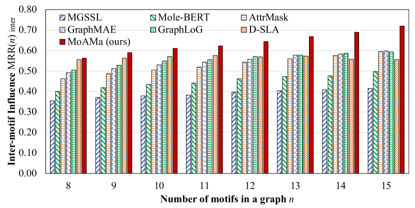
Figure 2: Inter-motif knowledge transfer score by motif count. A higher $\text{MRR}_{\text{inter}}^{(n)}$ score denotes greater inter-motif knowledge transfer.

Let $\{M_{1},...,M_{i},...,M_{n}\}$ be an ordered set, where $M_{i}\in\mathcal{M}$ and $s_{\text{motif}}(v,M_{i})\geq s_{\text{motif}}(v,M_{j})$ if $i<j$. Then we define $\text{rank}_{v}=i$ if $M_{i}=M_{v}$. Note that graphs with only $1$ motif are excluded as the distinction between inter and intra-motif nodes loses meaning. From this ranking, we define our score for inter-motif node influence averaged at the node, motif, and graph levels, derived from a similar score measurement used in information retrieval, Mean Reciprocal Rank (MRR) [37]:

$$\text{MRR}_{\text{node}} = \frac{1}{\sum_{(\mathcal{V},\mathcal{E})\in\mathcal{G}}|\mathcal{V}|}\sum_{(\mathcal{V},\mathcal{E})\in\mathcal{G}}\sum_{v\in\mathcal{V}}\frac{1}{\text{rank}_{v}},$$ (13)

$$\text{MRR}_{\text{graph}} = \frac{1}{|\mathcal{G}|}\sum_{(\mathcal{V},\mathcal{E})\in\mathcal{G}}\frac{1}{|\mathcal{V}|}\sum_{v\in\mathcal{V}}\frac{1}{\text{rank}_{v}}$$ (14)

$$\text{MRR}_{\text{motif}} = \sum_{n=2}^{N}\frac{|\mathcal{G}^{(n)}|}{|\mathcal{G}|\sum_{(\mathcal{V},\mathcal{E})\in\mathcal{G}^{(n)}}|\mathcal{V}|}\sum_{(\mathcal{V},\mathcal{E})\in\mathcal{G}^{(n)}}\sum_{v\in\mathcal{V}}\frac{1}{\text{rank}_{v}},$$ (15)

where $\mathcal{G}^{(n)}\subset\mathcal{G}$ is the set of graphs that contain $n\in[2,...,N]$ motifs.

Similar to the InfRatio measurements, $\text{MRR}_{\text{node}}$ directly captures the impact of the influence ranks for each node within the full graph set, whereas $\text{MRR}_{\text{graph}}$ alleviates bias on the number of nodes within a graph by averaging across individual graphs first. Because these rank-based measurements are intrinsically dependent on the number of motifs within each graph, we additionally define $\text{MRR}_{\text{motif}}$ which weights the measurement towards popular motif counts within the data distribution.

In information retrieval, MRR scores are used to quantify how well a system can return the most relevant item for a given query. Higher MRR scores indicate that relevant items were returned at higher ranks for each query. However, for our measurement, lower scores are preferred as lower intra-motif influence rank indicate greater inter-motif node influence. As opposed to traditional MRR measurements, where a higher rank for the most relevant item indicates better performance, we wish for the rank of the intra-motif influence, $s_{\text{inter}}(v)$, to be lower.

For the sake of clear visualization, we define an inter-motif score which indicates inter-motif knowledge transfer according to the number of motifs $n$ within a graph:

$$\text{MRR}^{(n)}_{\text{inter}}=1-\frac{1}{\sum_{(\mathcal{V},\mathcal{E})\in\mathcal{G}^{(n)}}|\mathcal{V}|}\sum_{(\mathcal{V},\mathcal{E})\in\mathcal{G}^{(n)}}\sum_{v\in\mathcal{V}}\frac{1}{\text{rank}_{v}}.$$ (16)

Figure 2 shows that our method outperforms all other models in terms of inter-motif knowledge transfer as shown by the higher $\text{MRR}_{\text{inter}}^{(n)}$ scores across different motif counts. Additionally, the inter-motif knowledge transfer using our method becomes more pronounced on graphs with higher numbers of motifs.

Table 3: Measurements of inter-motif knowledge transfer using different pre-trained models. A higher ratio is preferred for the InfRatio measurements, and a lower score is preferred for the MRR measurements.

Model	Avg Test AUC	$\text{InfRatio}_{\text{node}}$ $\uparrow$	$\text{InfRatio}_{\text{graph}}$ $\uparrow$	$\text{MRR}_{\text{node}}$ $\downarrow$	$\text{MRR}_{\text{graph}}$ $\downarrow$	$\text{MRR}_{\text{motif}}$ $\downarrow$
AttrMask	70.8	0.70	0.44	0.66	0.64	0.51
MGSSL	72.3	0.60	0.38	0.77	0.75	0.64
GraphLoG	73.4	0.79	0.50	0.61	0.59	0.48
D-SLA	73.8	0.76	0.49	0.67	0.66	0.44
GraphMAE	73.9	0.76	0.48	0.64	0.61	0.49
Mole-BERT	74.0	0.66	0.42	0.72	0.70	0.59
MoAMa	75.3	0.80	0.51	0.59	0.55	0.41

Additionally, in Table 3 we report the two InfRatio and three MRR measurements for our model and several baselines. A higher influence ratio indicates that inter-motif nodes have a greater effect on the target node. The relatively low values indicate that the intra-motif node influence is still highly important for the pre-training task, but our method demostrates the highest inter-motif knowledge transfer amongst the baselines. We see that there is a small positive correlation between the average test AUC for each model and the InfRatio measurements, with a Pearson correlation coefficient of 0.52 and 0.55 for the node and graph measurements, respectively, which supports our claim that greater inter-motif knowledge transfer leads to higher predictive performance. For the MRR measurements, our method boasts the lowest scores, which indicates less intra-motif knowledge dependence and greater inter-motif knowledge transfer. Again, the strength of inter-motif knowledge is supported by the observation of a small negative correlation between the average test AUC and the three MRR scores, with correlation coefficients of -0.39, -0.42, and -0.44 for the node, graph, and motif MRR measurements, respectively.

6 Conclusions

In this work, we introduced a novel motif-aware attribute masking strategy for attribute reconstruction during graph model pre-training. This motif-aware masking strategy outperformed existing methods that used random attribute masking, and achieved competitive results with the state-of-the-art methods because of the explicit transfer of inter-motif knowledge and intra-motif structural information. Our strategy also verified the methods of previous works to address limitations of previous graph pre-training methods, being training collapse and a lack of model expressivity.

For future work, it would be compelling to be able to encode global structure information using a motif-level message propagation method or gated attention units to capture long-distance motif dependencies, without relying on Tanimoto similarity.

Additionally, our method relies on specific domain knowledge when creating the chemical motif vocabulary. A more general graph decomposition method will be necessary to expand this strategy to other graph applications, such as networks. At the cost of computational resources, a strategy using a learned motif vocabulary may be able to generate motifs that are semantically meaningful but not yet utilized by domain experts.

References

- [1] Zhenqin Wu, Bharath Ramsundar, Evan Feinberg, Joseph Gomes, Caleb Geniesse, Aneesh Pappu, Karl Leswing, and Vijay Pande. Moleculenet: A benchmark for molecular machine learning. Chemical Science, 9, 03 2017.
- [2] Rees Chang, Yu-Xiong Wang, and Elif Ertekin. Towards overcoming data scarcity in materials science: unifying models and datasets with a mixture of experts framework, 2022.
- [3] Yanqiao Zhu, Yichen Xu, Qiang Liu, and Shu Wu. An empirical study of graph contrastive learning. arXiv preprint arXiv:2109.01116, 2021.
- [4] Weihua Hu, Bowen Liu, Joseph Gomes, Marinka Zitnik, Percy Liang, Vijay Pande, and Jure Leskovec. Strategies for pre-training graph neural networks, 2020.
- [5] Thomas N. Kipf and Max Welling. Variational graph auto-encoders, 2016.
- [6] Jun Xia, Yanqiao Zhu, Yuanqi Du, and Stan Z. Li. A survey of pretraining on graphs: Taxonomy, methods, and applications, 2022.
- [7] Kaiming He, Xinlei Chen, Saining Xie, Yanghao Li, Piotr Dollár, and Ross Girshick. Masked autoencoders are scalable vision learners. In Proceedings of the IEEE/CVF Conference on Computer Vision and Pattern Recognition, pages 16000–16009, 2022.
- [8] Jacob Devlin, Ming-Wei Chang, Kenton Lee, and Kristina Toutanova. Bert: Pre-training of deep bidirectional transformers for language understanding. arXiv preprint arXiv:1810.04805, 2018.
- [9] Phillip Pope, Soheil Kolouri, Mohammad Rostrami, Charles Martin, and Heiko Hoffmann. Discovering molecular functional groups using graph convolutional neural networks, 2019.
- [10] Jean MJ Frechet. Functional polymers and dendrimers: reactivity, molecular architecture, and interfacial energy. Science, 263(5154):1710–1715, 1994.
- [11] Merichel Plaza, Tania Pozzo, Jiayin Liu, Kazi Zubaida Gulshan Ara, Charlotta Turner, and Eva Nordberg Karlsson. Substituent effects on in vitro antioxidizing properties, stability, and solubility in flavonoids. Journal of agricultural and food chemistry, 62(15):3321–3333, 2014.
- [12] Ziniu Hu, Yuxiao Dong, Kuansan Wang, Kai-Wei Chang, and Yizhou Sun. Gpt-gnn: Generative pre-training of graph neural networks, 2020.
- [13] Shirui Pan, Ruiqi Hu, Guodong Long, Jing Jiang, Lina Yao, and Chengqi Zhang. Adversarially regularized graph autoencoder for graph embedding, 2019.
- [14] Zhenyu Hou, Xiao Liu, Yukuo Cen, Yuxiao Dong, Hongxia Yang, C. Wang, and Jie Tang. Graphmae: Self-supervised masked graph autoencoders. Proceedings of the 28th ACM SIGKDD Conference on Knowledge Discovery and Data Mining, 2022.
- [15] Seongjun Yun, Seoyoon Kim, Junhyun Lee, Jaewoo Kang, and Hyunwoo J Kim. Neo-gnns: Neighborhood overlap-aware graph neural networks for link prediction. In M. Ranzato, A. Beygelzimer, Y. Dauphin, P.S. Liang, and J. Wortman Vaughan, editors, Advances in Neural Information Processing Systems, volume 34, pages 13683–13694. Curran Associates, Inc., 2021.
- [16] Uri Alon and Eran Yahav. On the bottleneck of graph neural networks and its practical implications, 2021.
- [17] Gang Liu, Eric Inae, Tong Zhao, Jiaxin Xu, Tengfei Luo, and Meng Jiang. Data-centric learning from unlabeled graphs with diffusion model. arXiv preprint arXiv:2303.10108, 2023.
- [18] Zaixin Zhang, Qi Liu, Hao Wang, Chengqiang Lu, and Chee-Kong Lee. Motif-based graph self-supervised learning for molecular property prediction. In Neural Information Processing Systems, 2021.
- [19] Dongki Kim, Jinheon Baek, and Sung Ju Hwang. Graph self-supervised learning with accurate discrepancy learning. ArXiv, abs/2202.02989, 2022.
- [20] Jun Xia, Chengshuai Zhao, Bozhen Hu, Zhangyang Gao, Cheng Tan, Yue Liu, Siyuan Li, and Stan Z. Li. Mole-BERT: Rethinking pre-training graph neural networks for molecules. In The Eleventh International Conference on Learning Representations, 2023.
- [21] Yu Rong, Yatao Bian, Tingyang Xu, Weiyang Xie, Ying Wei, Wenbing Huang, and Junzhou Huang. Self-supervised graph transformer on large-scale molecular data. In Proceedings of the 34th International Conference on Neural Information Processing Systems, NIPS’20, Red Hook, NY, USA, 2020. Curran Associates Inc.
- [22] Mengying Sun, Jing Xing, Huijun Wang, Bin Chen, and Jiayu Zhou. Mocl: Data-driven molecular fingerprint via knowledge-aware contrastive learning from molecular graph. In Proceedings of the 27th ACM SIGKDD Conference on Knowledge Discovery & Data Mining, KDD ’21, page 3585–3594, New York, NY, USA, 2021. Association for Computing Machinery.
- [23] Yuning You, Tianlong Chen, Yongduo Sui, Ting Chen, Zhangyang Wang, and Yang Shen. Graph contrastive learning with augmentations. Advances in neural information processing systems, 33:5812–5823, 2020.
- [24] Yuning You, Tianlong Chen, Yang Shen, and Zhangyang Wang. Graph contrastive learning automated. In International Conference on Machine Learning, pages 12121–12132. PMLR, 2021.
- [25] Keyulu Xu, Weihua Hu, Jure Leskovec, and Stefanie Jegelka. How powerful are graph neural networks? In 7th International Conference on Learning Representations, ICLR 2019, New Orleans, LA, USA, May 6-9, 2019. OpenReview.net, 2019.
- [26] Jörg Degen, Christof Wegscheid-Gerlach, Andrea Zaliani, and Matthias Rarey. On the art of compiling and using ’drug-like’ chemical fragment spaces. ChemMedChem, 3, 2008.
- [27] Zijie Geng, Shufang Xie, Yingce Xia, Lijun Wu, Tao Qin, Jie Wang, Yongdong Zhang, Feng Wu, and Tie-Yan Liu. De novo molecular generation via connection-aware motif mining. arXiv preprint arXiv:2302.01129, 2023.
- [28] T. Sterling and John J. Irwin. Zinc 15 – ligand discovery for everyone. Journal of Chemical Information and Modeling, 55:2324 – 2337, 2015.
- [29] Dávid Bajusz, Anita Rácz, and Károly Héberger. Why is tanimoto index an appropriate choice for fingerprint-based similarity calculations? Journal of Cheminformatics, 7, 2015.
- [30] Yifei Wang, Shiyang Chen, Guobin Chen, Ethan Shurberg, Hang Liu, and Pengyu Hong. Motif-based graph representation learning with application to chemical molecules, 2022.
- [31] Minghao Xu, Hang Wang, Bingbing Ni, Hongyu Guo, and Jian Tang. Self-supervised graph-level representation learning with local and global structure. In Marina Meila and Tong Zhang, editors, Proceedings of the 38th International Conference on Machine Learning, volume 139 of Proceedings of Machine Learning Research, pages 11548–11558. PMLR, 18–24 Jul 2021.
- [32] Chaoning Zhang, Chenshuang Zhang, Junha Song, John Seon Keun Yi, Kang Zhang, and In So Kweon. A survey on masked autoencoder for self-supervised learning in vision and beyond, 2022.
- [33] Mathieu Germain, Karol Gregor, Iain Murray, and Hugo Larochelle. Made: Masked autoencoder for distribution estimation, 2015.
- [34] Jiwoong Park, Minsik Lee, Hyung Jin Chang, Kyuewang Lee, and Jin Young Choi. Symmetric graph convolutional autoencoder for unsupervised graph representation learning. In Proceedings of the IEEE International Conference on Computer Vision, pages 6519–6528, 2019.
- [35] Amin Salehi and Hasan Davulcu. Graph attention auto-encoders, 2019.
- [36] Chun Wang, Shirui Pan, Guodong Long, Xingquan Zhu, and Jing Jiang. Mgae: Marginalized graph autoencoder for graph clustering. In Proceedings of the 2017 ACM on Conference on Information and Knowledge Management, CIKM ’17, page 889–898, New York, NY, USA, 2017. Association for Computing Machinery.
- [37] Nick Craswell. Mean Reciprocal Rank, pages 1703–1703. Springer US, Boston, MA, 2009.