Quantum Quenches of Conformal Field Theory with Open Boundary

Abstract

We develop a method to derive the exact formula of entanglement entropy for generic inhomogeneous conformal field theory (CFT) quantum quenches with open boundary condition (OBC), which characterizes the generic boundary effect unresolved by analytical methods in the past. We identify the generic OBC quenches with Euclidean path integrals in complicated spacetime geometries, and we show that a special class of OBC quenches, including the Möbius and sine-square-deformation quenches, have simple boundary effects calculable from Euclidean path integrals in a simple strip spacetime geometry. We verify that our generic CFT formula matches well with free fermion tight-binding model numerical calculations for various quench problems with OBC. Our method can be easily generalized to calculate any local quantities expressible as one-point functions in such quantum quench problems.

Recent developments in quantum devices and simulators enable us to explore far-from-equilibrium quantum dynamics of many-body systems, which is of both fundamental and practical importance. A paradigm is quantum quenches which have been studied extensively both theoretically and experimentally [1, 2, 3, 4, 5, 6, 7, 8, 9, 10, 11, 12, 13, 14, 15, 16, 17, 18] where a system initially in a stationary state of some Hamiltonian is time-evolved by another Hamiltonian. The post-quench evolution of entanglement entropy and other quantities can reflect intrinsic dynamical properties of many-body systems such as ergodicity/non-ergodicity. Particularly, quantum quenches with inhomogeneity from disorder or intentional modulation yield intriguing dynamics rather than a nuisance. For instance, square-root deformation (SRD) quench allows perfect distant quantum communication [19], while Möbius and sine-square deformation (SSD) quenches can lead to heating/non-heating dynamics and create a black-hole like excitation [20, 21].

Previous studies demonstrate that, a class of inhomogeneous quantum quench and Floquet problems in $(1+1)$d conformal field theory (CFT) are amendable to exact solutions – see, for example, [22, 23, 6, 24, 25, 26, 27, 28, 29, 30, 31, 32, 33, 34, 21, 35, 36]. For finite systems with periodic boundary condition (PBC) [21, 33, 34, 25], analytical formulas for generic smooth inhomogeneous quenches are derived, which reveal rich physics of inhomogeneous CFTs. However, for finite systems with open boundary condition (OBC), analytical solutions are only found for Möbius and SSD quenches [34, 25], while the generic inhomogeneous quench problems suffer from boundary effects and have not been solved.

In this letter, we study the entanglement entropy of generic inhomogeneous CFT quenches with OBC. We first show that they correspond to Euclidean path integrals in complicated spactime geometries difficult to calculate. We then develop a method circumventing this difficulty, and derive the exact formula characterizing the generic boundary effect. We also show that a special class of OBC quench problems, including Möbius and SSD quenches studied previously [34, 25], reduce to Euclidean path integrals in a simple strip spacetime geometry, which we say have simple boundary effect. We verify that our generic formula matches well with free fermion tight-binding calculations for various quench problems in Tab. 1. Our method permits straightforward generalizations to other physical quantities.

Setup. We consider a (1+1)d CFT with central charge $c$. The class of conformal quench problems of our interest is defined on a spatial interval $x\in[0,L]$ with OBC. The case of (semi)infinite interval can be derived by taking the limit $L\to\infty$. Initially, the system is in the ground state $|\psi_{0}\rangle$ of the uniform CFT Hamiltonian

$$H_{0}=\int_{0}^{L}h(x)dx\ ,$$ (1)

where $h(x)$ is the energy density. Starting from time $t=0$, the Hamiltonian is suddenly changed to

$$H=\int_{0}^{L}f(x)h(x)dx\ ,$$ (2)

where $f(x)$ is an arbitrary smooth real non-negative function for $x\in[0,L]$. The deformed Hamiltonians of this type have been studied for various choices of $f(x)$ [37, 38, 39, 40, 41, 42, 43, 44, 45, 46, 47, 48, 49, 50, 51, 52]. Our goal is to calculate the entanglement entropy $S_{A}(x,t)=-\text{tr}\left[\rho_{A}(t)\ln\rho_{A}(t)\right]$ of a subsystem $A$ defined as the interval $[0,x]$ (where $0<x<L$) at post-quench time $t\geq 0$. Here, $\rho_{A}(t)$ is the reduced density matrix of subsystem $A$ at time $t$.

Let us start by observing that, since the Hamiltonian generates time translation, the quench from $H_{0}$ to $H$ can be viewed as a sudden change of the metric from $ds_{0}^{2}$ to $ds^{2}$ at time $t=0$:

$$ds_{0}^{2}=-d\tilde{t}^{2}+d\tilde{x}^{2}\quad\rightarrow\quad ds^{2}=-f(x)^{2}dt^{2}+dx^{2}\ .$$ (3)

Here we use $(\tilde{x},\tilde{t})$ and $(x,t)$ to denote the spacetime coordinates before and after time $t=0$, respectively, with $\tilde{x}=x$ at $t=0$. This amounts to a change in the speed of light from $1$ to $f(x)$ at $t=0$.

To simplify this metric-changing quench problem, we first redefine the post-quench spatial coordinate $x$ into a coordinate $y$:

$$\frac{dy}{dx}=\frac{1}{f(x)},\quad y=\int^{x}\frac{dx^{\prime}}{f\left(x^{\prime}\right)}=g(x)\ ,$$ (4)

in which the post-quench speed of light is normalized back to $1$. To extend the coordinate $y$ into pre-quench times, we switch to Euclidean time $\tilde{t}=-i\tilde{\tau}$ and $t=-i\tau$, and assume $f(x)$ and thus $g(x)$ can be analytically continued into the complex plane. For the pre-quench spacetime, we perform a conformal transformation from complex coordinate $z=\tilde{x}+i\tilde{\tau}$ to $w=y+i\tau=g(z)$ (thus $dw/dz=f(z)^{-1}$). The metric $ds_{0}^{2}$ ($ds^{2}$) before (after) quench in Eq. 3 can then be rewritten in coordinates $(y,-i\tau)$ as

$$ds_{0}^{2}=|f(z)|^{2}\left(d\tau^{2}+dy^{2}\right)\ \rightarrow\ ds^{2}=f(x)^{2}\left(d\tau^{2}+dy^{2}\right)$$ (5)

Thus, coordinate $w=y+i\tau$ glues together the metrics $ds_{0}^{2}$ and $ds^{2}$ at $t=0$ without changing the speed of light.

For OBC, the post-quench entanglement entropy can be calculated using the replica trick from the twist operator one-point function [53]:

$$S_{A}(x,-i\tau)=-\lim_{n\rightarrow 1}\frac{\partial\,\text{tr}\left(\rho_{A}^{n}\right)}{\partial n}=-\lim_{n\rightarrow 1}\frac{\partial}{\partial n}\left\langle\mathcal{T}_{n}^{\prime}(w)\right\rangle\ \\$$ (6)

Here $\mathcal{T}_{n}^{\prime}(w)$ is the twist operator at the post-quench coordinate $w=y+i\tau=g(x)+i\tau$, and

$$\left\langle\mathcal{T}_{n}^{\prime}(w)\right\rangle=\mathrm{tr}\left[|\psi_{0}\rangle\langle\psi_{0}|e^{H\tau}\mathcal{T}_{n}^{\prime}(y)e^{-H\tau}\right]\ .$$ (7)

By writing the initial state $|\psi_{0}\rangle=\lim_{\beta\rightarrow\infty}e^{-\beta H_{0}}|\alpha\rangle$ with arbitrary state $|\alpha\rangle$, we can rewrite it in the pre-quench coordinate $z=\tilde{x}+i\tilde{\tau}$ as a path integral in a half-infinite strip $\mathcal{M}_{\text{gs}}^{<}$, defined as the $\widetilde{\tau}<0$ region of strip $\mathcal{M}_{\text{gs}}$ (manifold $\text{Re}(z)\in[0,L]$) in Fig. 1(a) with straight ($\tilde{\tau}$ independent) boundaries $\partial\mathcal{M}_{\text{gs}}$ at $\tilde{x}=0$ and $L$:

$$\langle\phi_{F}|\psi_{0}\rangle=\int_{\phi_{\tilde{\tau}=0}=\phi_{F}}D\phi e^{-\int_{-\infty}^{0}d\tilde{\tau}\int_{0}^{L}d\tilde{x}\mathcal{L}_{0}(\phi)}$$ (8)

Here $\mathcal{L}_{0}(\phi)$ is the uniform Lagrangian density corresponding to energy density $h(\tilde{x})$. If the conformal transformation $z\rightarrow w=g(z)$ maps the strip $\mathcal{M}_{\text{gs}}$ into a manifold $\mathcal{M}_{\text{gs}}^{\prime}$ in coordinate $w$ (grey region in Fig. 2(b)), the path integral in Eq. 8 becomes (SI [54] Sec. I):

$$\begin{split}\langle\phi_{F}^{\prime}|\psi_{0}\rangle=\int_{\phi_{\tau=0}^{\prime}=\phi_{F}^{\prime}}D\phi^{\prime}e^{-\int_{\mathcal{M}_{\text{gs}}^{\prime<}}d\tau dy\mathcal{L}_{0}^{\prime}\left(\phi^{\prime}\right)}\ ,\end{split}$$ (9)

where $\mathcal{M}_{\text{gs}}^{\prime<}$ denotes the $\tau<0$ region of manifold $\mathcal{M}_{\text{gs}}^{\prime}$, and the Lagrangian density $\mathcal{L}_{0}^{\prime}\left(\phi^{\prime}\right)=|f(z)|^{2}\mathcal{L}_{0}(\phi)$ remains uniform by conformal symmetry. In contrast, the time evolution operator $e^{-H\tau}=e^{-\tau\int_{0}^{L}f(x)h(x)dx}$ in Eq. 7 is equivalent to a path integral in coordinate $w$ in the blue rectangle in Fig. 1(b) (SI [54] Sec. I)

$$\begin{split}\langle\phi_{F}^{\prime}|e^{-H\tau}|\phi_{I}^{\prime}\rangle&=\int_{\phi_{\tau=0}^{\prime}=\phi_{I}^{\prime}}^{\phi_{\tau}^{\prime}=\phi_{F}^{\prime}}D\phi^{\prime}e^{-\int_{0}^{\tau}d\tau^{\prime}\int_{y_{L}}^{y_{R}}dy\mathcal{L}_{0}^{\prime}\left(\phi^{\prime}\right)}\end{split}$$ (10)

where $y_{L}=g(0)$ and $y_{R}=g(L)$ are the straight ($\tau$ independent) physical boundary in coordinate $y$ after quench, denoted by $\partial\mathcal{M}_{\text{phy}}^{\prime}$ in Fig. 1(b). By Eqs. 9 and 10, we can rewrite Eq. 7 as a path integral in a manifold of $\mathcal{M}_{\text{gs}}^{\prime}$ glued with two rectangles in the order $1\rightarrow 2\rightarrow 3\rightarrow 4$ as shown in Fig. 1(b), with the twist operator inserted between rectangles $1$ and $2$, which has a complicated spacetime geometry.

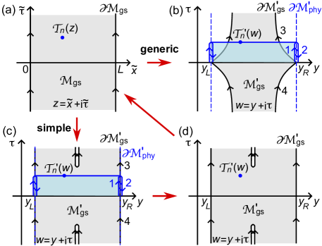
Figure 1: (a) The initial state path integral manifold $\mathcal{M}_{\text{gs}}$ in $z$ coordinate. (b) Path integral representation ($1\rightarrow 2\rightarrow 3\rightarrow 4$) for Eq. 7 in $w=y+i\tau$ coordinate. (c) Panel (b) for the Möbius quench, which can be reduced to (d).

Simple boundary effect. For a simple class of functions $f(x)$, the two boundaries $\partial\mathcal{M}_{\text{phy}}^{\prime}$ and $\partial\mathcal{M}_{\text{gs}}^{\prime}$ exactly match within a finite Euclidean time interval $(-\tau_{0},\tau_{0})$. This includes the case $y_{L}=-\infty$ ($y_{R}=\infty$), where $\partial\mathcal{M}_{\text{phy}}^{\prime}$ and $\partial\mathcal{M}_{\text{gs}}^{\prime}$ around $y_{L}$ ($y_{R}$) are infinitely away and effectively match. An example is the previously studied Möbius quench (Tab. 1) shown in Fig. 1(c). In this case, for $\tau\in(-\tau_{0},\tau_{0})$, the path integral in rectangle $2$ cancels with part of $3$, thus Eq. 7 reduces to a path integral simply in the manifold $\mathcal{M}_{\text{gs}}^{\prime}$ in Fig. 1(d). By an inverse conformal mapping $z=g^{-1}(w)$, one can map $\mathcal{M}_{\text{gs}}^{\prime}$ back to the simple strip geometry $\mathcal{M}_{\text{gs}}$ in Fig. 1(a), in which the twist operator one-point function $\left\langle\mathcal{T}_{n}(z)\right\rangle_{\mathcal{M}_{\text{gs}}}$ can be easily calculated and is translationally invariant in $\tilde{\tau}$. We thus have

$$\langle\mathcal{T}_{n}^{\prime}(w)\rangle=\left|\frac{dw}{dz}\right|^{-\Delta_{n}}\left\langle\mathcal{T}_{n}(z)\right\rangle_{\mathcal{M}_{\text{gs}}}\ ,$$ (11)

where $\Delta_{n}=\frac{c}{12}(n-\frac{1}{n})$ is the twist operator scaling dimension. The entanglement entropy can then be derived from Eq. 6 as (See SI [54] Sec. II)

$$\begin{split}S_{A}(x,-i\tau)&=\frac{c}{6}\ln\left[\frac{|dw/dz|_{\tau}}{|dw/dz|_{\tau=0}}\frac{2L}{\pi\epsilon}\sin\frac{\pi\tilde{x}\left(y,\tau\right)}{L}\right]\end{split}$$ (12)

where $\tilde{x}(y,\tau)=\text{Re}(z)=\text{Re}\left[g^{-1}(w)\right]$, and $y=g(x)$. The formula has an ultraviolet (UV) cutoff $\epsilon|dw/dz|_{\tau=0}$, which is fixed by the constraint that $S_{A}$ at time $t=-i\tau=0$ matches with the entanglement entropy of the initial state $|\psi_{0}\rangle$.

The analyticity of Eq. 12 in $\tau\in(-\tau_{0},\tau_{0})$ ensures its analytical continuation to real time $t\geq 0$:

$$\begin{split}S_{A}=\frac{c}{6}\ln\left[\left(\frac{\partial x_{+}}{\partial x}\frac{\partial x_{-}}{\partial x}\right)^{-\frac{1}{2}}\frac{2L}{\pi\epsilon}\sin\frac{\pi\left(x_{+}+x_{-}\right)}{2L}\right]\end{split}$$ (13)

where $x_{\pm}=g^{-1}(y_{\pm})=g^{-1}(g(x)\mp t)$ are the light cone coordinates, which can be viewed as the initial positions of a quasiparticle moving at velocities $\pm f(x)$ reaching position $x$ at time $t$. As shown in SI [54] Sec. IV, $g^{-1}(y)$ in this case has analytical continuation on the entire real axis $y\in\mathbb{R}$, thus Eq. 13 holds for all $t\geq 0$.

We say this class of OBC quenches obeying Eq. 13 have simple boundary effect, which reduce to simple calculations in a strip in Fig. 1(a). Particularly, if $\partial\mathcal{M}_{\text{phy}}^{\prime}$ and $\partial\mathcal{M}_{\text{gs}}^{\prime}$ match entirely (only true for half Möbius quench, see SI [54] Sec. VI), quench dynamics will be absent due to the $\tau$ translation symmetry.

Generic boundary effect. For generic functions $f(x)$, boundaries $\partial\mathcal{M}_{\text{phy}}^{\prime}$ and $\partial\mathcal{M}_{\text{gs}}^{\prime}$ may mismatch almost everywhere as shown in Fig. 1(b), invalidating the derivation of Eq. 13. Accordingly, we numerically find that the analytical continuation of Eq. 13 fails when $x_{\pm}=g^{-1}(g(x)\mp t)$ lies beyond the physical boundary of space $[0,L]$. The above observations in both Euclidean and real times imply that such OBC quenches no longer have simple boundary effect given by Eq. 13, and we say they have generic boundary effect.

We now show how to remediate Eq. 13 to derive the generic boundary effect. We first define the light cone coordinates $x_{\pm}\in[0,L]$ as initial positions of a quasiparticle reaching point $(x,t)$ from the left/right. By rewriting $g(x)\mp t-y_{L}=\mp n_{\pm}(y_{R}-y_{L})+q_{\pm}$ with $n_{\pm}\in\mathbb{Z}$ and $q_{\pm}\in[0,y_{R}-y_{L})$, we explicitly have

$$x_{\pm}=g^{-1}(y_{\pm})\ ,\quad y_{\pm}=\begin{cases}&y_{L}+q_{\pm}\ \left(n_{\pm}\text{ even}\right)\\ &y_{R}-q_{\pm}\ \left(n_{\pm}\text{ odd}\right)\end{cases},$$ (14)

where $n_{\pm}$ is the number of reflections by physical boundary the quasiparticle experienced, as shown in Fig. 2(a)-(b).

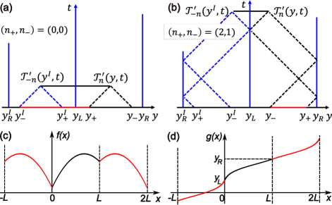
Figure 2: (a)-(b): The ancillary mirror PBC system for the OBC system in $y$ coordinates for the examples of $(n_{+},n_{-})=(0,0)$ and $(2,1)$. Index $I$ stands for mirror image. (c)-(d) The equivalent mirror extensions of $f(x)$ and $g(x)$ to $x\in\mathbb{R}$.

Secondly, we define an ancillary mirror PBC quench system with period $2L$ in $x$, where intervals $[0,L]$ and $[-L,0]$ are our OBC quench system and its mirror copy, respectively. In $y$ coordinate, the OBC one-point function Eq. 7 can be expressed as $\langle\mathcal{T}_{n}^{\prime}(y,t)\rangle=\sqrt{\langle\mathcal{T}_{n}^{\prime}(y,t)\mathcal{T}_{-n}^{\prime}(y^{I},t)\rangle_{\text{mp}}}$ using the two-point function between $\mathcal{T}_{n}^{\prime}$ at $(y,t)$ and its image $\mathcal{T}_{-n}^{\prime}$ at $(y^{I},t)$ in the mirror PBC system (Fig. 2(a)-(b)). Accordingly, entanglement entropy $S_{A}$ of the OBC system is half of that in interval $[y^{I},y]$ of its mirror PBC system at time $t$.

For the boundaryless mirror PBC system, the interval $[y^{I},y]$ at time $t$ are right-propagated from the red interval in Fig. 2(a)-(b) at time $t=0$, and left-propagated from its image. In the $x$ coordinate, $y_{\pm}^{I}$ as images of $y_{\pm}$ map to $-x_{\pm}=-g^{-1}(y_{\pm})$, and one can prove the red interval, or its complement in the period $2L$ space, has a length $\left|x_{+}+(-1)^{n_{-}-n_{+}}x_{-}\right|$ (see examples of Fig. 2(a)-(b)). This gives the OBC $S_{A}$ from the two-point function across the red interval of initial PBC ground state and the Jacobians $\frac{\partial x_{\pm}}{\partial x}$ as (See SI [54] Sec. III):

$$\begin{split}&S_{A}=\frac{c}{6}\ln\left[\left|\frac{\partial x_{+}}{\partial x}\frac{\partial x_{-}}{\partial x}\right|^{-\frac{1}{2}}\frac{2L}{\pi\epsilon}\sin\frac{\pi\left|x_{+}+(-1)^{n_{-}-n_{+}}x_{-}\right|}{2L}\right]\end{split}$$ (15)

Eq. 15 gives the exact generic boundary effect, with $x_{\pm}$ defined in Eq. 14.

The ancillary mirror PBC extension for deriving Eq. 15 is equivalent to the mirror extension of $f(x)$ from $x\in[0,L]$ into $x\in\mathbb{R}$ as an even function with period $2L$, and accordingly $g(x)$ into $x\in\mathbb{R}$ by Eq. 4, as illustrated in Fig. 2(c)-(d). Such an extension of $f(x)$ and $g(x)$ is clearly not an analytical continuation, thus the analytical continuation of Eq. 13 generically fails.

Meanwhile, this indicates the condition for Eq. 15 to reduce to the simple boundary effect in Eq. 13 is that, the analytical continuation of $f(x)$ in $x\in\mathbb{R}$ is even and $2L$ periodic. Earlier, we derived Eq. 13 from a different condition that, the two boundaries $\partial\mathcal{M}_{\text{phy}}^{\prime}$ and $\partial\mathcal{M}_{\text{gs}}^{\prime}$ match within a finite Euclidean time interval $(-\tau_{0},\tau_{0})$. In fact, these two conditions are equivalent, which is proved in SI [54] Sec. IV. This fully clarifies the simple boundary effect from both Euclidean and real time perspectives.

Numerical verification. To check against Eq. 15, we numerically calculate the entanglement entropy of an OBC free fermion tight-binding model with quench function $f(x)$ [55]. It has Hamiltonian $H_{0}=-\frac{1}{2}\sum_{j=1}^{L-1}\left(c_{j+1}^{\dagger}c_{j}+h.c.\right)$ before quench, and $H=-\frac{1}{2}\sum_{j=1}^{L-1}\left[f(j)c_{j+1}^{\dagger}c_{j}+h.c.\right]$ after quench, where $c_{j},c_{j}^{\dagger}$ are the site-$j$ fermion annihilation/creation operators. We fix the filling at $\nu=\frac{1}{2}$, such that its low energy theory is a CFT with the speed of light $1$ before quench, and central charge $c=1$.

Quench	$f(x)$ for $x\in[0,L]$	$g(x)$ for $x\in[0,L]$
tEH	$\frac{\left(x+L_{1}\right)\left(L+L_{2}-x\right)}{L+L_{1}+L_{2}}$	$\ln\left(\frac{x+L_{1}}{L+L_{2}-x}\right)$
tSRD	$\sqrt{\left(x+L_{1}\right)\left(L+L_{2}-x\right)}$	$\cos^{-1}{\left(\frac{L+L_{2}-L_{1}-2x}{L+L_{1}+L_{2}}\right)}$
Rainbow	$e^{-kx}$, $x\in[0,L]$	$\frac{e^{kx}}{k}$
Möbius	$1-\lambda\cos(\frac{2\pi x}{L})$	$-\frac{L_{\text{eff }}}{\pi}\tan^{-1}\left(\frac{a}{\tan\frac{\pi x}{L}}\right)$

Table 1: Quench functions calculated. For Möbius quench, $L_{\text{eff}}=\frac{L}{\sqrt{1-\lambda^{2}}}$, $a=\frac{\sqrt{1-\lambda^{2}}}{1+\lambda}$, and taking $\lambda\rightarrow 1$ gives the SSD quench.

We calculate the truncated entanglement Hamiltonian (tEH), truncated SRD (tSRD), rainbow and Möbius (which includes SSD as a limit) quenches [40, 51, 52, 39], for which $f(x)$ and $g(x)$ are listed in Tab. 1 (See SI [54] Sec. VI). When $L_{1}=L_{2}=0$, tEH and tSRD reduce to the entanglement Hamiltonian (EH) and SRD quenches in literature [51]. As shown in Fig. 3 and SI [54] Fig. S2, $S_{A}(x,t)$ with respect to $x$ or $t$ from the CFT formula Eq. 15 (blue lines) and from the tight-binding calculations (red circles) match well, except that the tight-binding data show an additional filling $\nu$ dependent period $\frac{1}{\nu}=2$ oscillation in $x$ (which is UV physics).

The EH quench shown in Fig. 3(a) has simple boundary effect since $y_{L}=-\infty$ and $y_{R}=\infty$. Its $S_{A}(x,t)$ from the CFT Eq. 15 is in a heating phase with perpetual linear growth in $t$, because there exist hot spots $x=0$ and $x=L$ [25, 34, 56]. A hot spot $x_{h}\in[0,L]$ is where $f(x)\propto|x-x_{h}|^{\eta}$ with $\eta\geq 1$, thus the time $\int^{x_{h}}\frac{dx}{f(x)}$ for particles to reach $x_{h}$ diverges, and heat (entropy) is trapped at $x_{h}$. $S_{A}(x,t)$ from tight-binding calculations is eventually upper bounded at large $t$, as the spatial UV cutoff (lattice constant) around the hot spots prevents the time divergence.

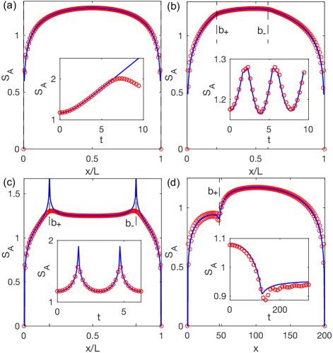
Figure 3: Numerical comparison between the CFT Eq. 15 with a fixed fitted $\epsilon$ (blue lines) and free-fermion tight-binding calculation (red circles), all for system size $L=200$. Each panel shows $S_{A}(x,t_{0})$ at a fixed time $t=t_{0}$, and the inset shows $S_{A}(x_{0},t)$ at a fixed position $x=x_{0}$. The quenches and parameters are: (a) EH (tEH with $L_{1}=L_{2}=0$), $t_{0}=\frac{9\pi}{20}$, $x_{0}=0.5L$. (b) tEH with $L_{1}=0.1L$, $L_{2}=0.3L$, $t_{0}=\frac{9\pi}{20}$, $x_{0}=0.5L$. (c) SRD (tSRD with $L_{1}=L_{2}=0$), $t_{0}=\frac{3\pi}{10}$, $x_{0}=0.5L$. (d) Rainbow (finite $L$) with $k=0.05$, $t_{0}=60\pi$, $x_{0}=40$. More examples (including Möbius and SSD) are shown in SI [54] Fig. S2.

Fig. 3(b)-(d) shows the tEH ($L_{1},L_{2}>0$), SRD and rainbow quenches which have generic boundary effect. They have $\partial_{x}S_{A}(x,t)$ discontinuities (from the Jacobian $\frac{\partial x_{\pm}}{\partial x}$ in Eq. 15) at the vertical dashed line positions $b_{+}=g^{-1}(y_{L}+t)$ and $b_{-}=g^{-1}(y_{R}-t)$. This is because $x=b_{\pm}$ is where $x_{\pm}$ hits the physical boundary, and $n_{\pm}$ changes by $1$. Therefore, the discontinuities at $b_{\pm}$ can be viewed as the shock fronts from boundary reflections. For SRD (Fig. 3(c)), the CFT formula shows divergent discontinuities. While tight-binding results cannot diverge due to spatial UV cutoff, they approach the CFT formula as $L\rightarrow\infty$. For simple boundary effect (EH in Fig. 3(a), Möbius and SSD in SI [54] Fig. S2), $S_{A}(x,t)$ is analytical without discontinuities at any $x\in(0,L)$.

Discussion. Our method solves both simple and generic boundary effects of CFT quenches with OBC, which correspond to simple and complicated Euclidean path-integral spacetime geometries, respectively. The ancillary mirror PBC picture we developed implies that, the previous solution for CFT quenches with PBC [33] also corresponds to simple Euclidean path-integral spacetime geometries, which we prove in SI [54] Sec. V. Although we only derived entanglement entropy (Eq. 15) for generic OBC quenches, our method easily generalizes to any local quantities calculable as one-point functions. Our method allows studies of generic quench problems in quantum simulators such as Rydberg atom arrays [57, 58, 59, 60, 61, 62], which can be tuned to conformal critical points. Moreover, an intriguing future question is to extend our method to generic time-dependent problems, such as moving mirror and Floquet dynamics problems [31, 32, 34, 25, 63, 24, 64].

Supplementary Material

.1 I. The twist operator one-point function in the Euclidean path integral picture

By expressing the initial state as $|\psi_{0}\rangle=\lim_{\beta\rightarrow\infty}e^{-\beta H_{0}}|\alpha\rangle$ with arbitrary state $|\alpha\rangle$, we can rewrite it in the pre-quench coordinate $z=\tilde{x}+i\tilde{\tau}$ as a path integral in a half-infinite strip $\mathcal{M}_{\text{gs}}^{<}$, defined as the $\widetilde{\tau}<0$ region of strip $\mathcal{M}_{\text{gs}}$ in the main text Fig. 1(a) with straight boundaries $\partial\mathcal{M}_{\text{gs}}$ at $\tilde{x}=0$ and $L$:

$$\langle\phi_{F}|\psi_{0}\rangle=\int_{\phi_{\tilde{\tau}=0}=\phi_{F}}D\phi e^{-\int_{-\infty}^{0}d\tilde{\tau}\int_{0}^{L}d\tilde{x}\mathcal{L}_{0}(\phi)}\ ,$$ (S1)

where $\phi(\tilde{x},\tilde{\tau})$ represents all the quantum fields in the CFT. The uniform Lagrangian $\mathcal{L}_{0}(\phi(\tilde{x},\tilde{\tau}))$ lives in the strip $\tilde{x}\in[0,L]$, and is the Legendre transformation of the uniform energy density $h(\tilde{x})$.

Since the theory we consider is CFT, the Lagrangian density $\mathcal{L}_{0}(\phi)$ has scaling dimension 2. Therefore, under conformal mapping $z\rightarrow w=g(z)$, with $dw/dz=dg(z)/dz=1/f(z)$:

$$\begin{split}\mathcal{L}_{0}(\phi(z))\longrightarrow\frac{1}{|f(z)|^{2}}\mathcal{L}_{0}^{\prime}\left(\phi^{\prime}(w)\right)\ ,\qquad d\tilde{\tau}d\tilde{x}=|dz|^{2}=|f(z)|^{2}|dw|^{2}=|f(z)|^{2}d\tau dy\ ,\end{split}$$ (S2)

so the action of the path integral Eq. S1 transforms as

$$\begin{split}&\int_{-\infty}^{0}d\tilde{\tau}\int_{0}^{L}d\tilde{x}\mathcal{L}_{0}(\phi)=\int_{\mathcal{M}_{\text{gs}}^{\prime<}}d\tau dy|f(z)|^{2}\frac{1}{|f(z)|^{2}}\mathcal{L}_{0}^{\prime}\left(\phi^{\prime}\right)=\int_{\mathcal{M}_{\text{gs}}^{\prime<}}d\tau dy\mathcal{L}_{0}^{\prime}\left(\phi^{\prime}\right)\end{split}$$ (S3)

where the new Lagrangian $\mathcal{L}_{0}^{\prime}\left(\phi^{\prime}\right)$ is still uniform in spacetime due to conformal symmetry, and $\phi^{\prime}(w)$ represents quantum fields in the $w$ coordinate. Here $\mathcal{M}_{\text{gs}}^{\prime<}$ denotes the $\tau<0$ region of the manifold $\mathcal{M}_{\text{gs}}^{\prime}$ in main text Fig. 1(b), and it has curved boundaries $\partial\mathcal{M}_{\text{gs}}^{\prime}$ mapped from the straight boundaries $\partial\mathcal{M}_{\text{gs}}$ in main text Fig. 1(a). The path integral for the initial state now becomes

$$\begin{split}\langle\phi_{F}^{\prime}|\psi_{0}\rangle=\int_{\phi_{\tau=0}^{\prime}=\phi_{F}^{\prime}}D\phi^{\prime}e^{-\int_{\mathcal{M}_{\text{gs}}^{\prime<}}d\tau dy\mathcal{L}_{0}^{\prime}\left(\phi^{\prime}\right)}\ ,\end{split}$$ (S4)

Meanwhile, the conformal mapping $z\rightarrow w=g(z)$ also maps the energy density (which has scaling dimension $2$) as

$$h(z)=\frac{1}{|f(z)|^{2}}h^{\prime}(w)\ ,$$ (S5)

where $h^{\prime}(w)$ is the uniform energy density in the $w=y+i\tau$ coordinates. In particular, at time $\tau=it=0$, one has $w=y$, and the corresponding $z=\tilde{x}=x$ (recall that coordinates $\tilde{x}$ and $x$ match at time $t=0$), so Eq. S5 implies

$$h(x)=\frac{1}{|f(x)|^{2}}h^{\prime}(y)\ .$$ (S6)

Therefore, the post-quench time evolution operator $e^{-H\tau}$ of $|\psi_{0}\rangle$ can be transformed into the $(\tau,y)$ coordinates as

$$\begin{split}e^{-H\tau}&=e^{-\tau\int_{0}^{L}f(x)h(x)dx}=e^{-\tau\int_{y_{L}}^{y_{R}}h^{\prime}(y)dy}\ ,\end{split}$$ (S7)

where we have used Eq. S6 and the fact that $dx=f(x)dy$. This is equivalent to a path integral in coordinate $w=y+i\tau$ with straight boundaries

$$\begin{split}\langle\phi_{F}^{\prime}|e^{-H\tau}|\phi_{I}^{\prime}\rangle&=\int_{\phi_{\tau=0}^{\prime}=\phi_{I}^{\prime}}^{\phi_{\tau}^{\prime}=\phi_{F}^{\prime}}D\phi^{\prime}e^{-\int_{0}^{\tau}d\tau^{\prime}\int_{y_{L}}^{y_{R}}dy\mathcal{L}_{0}^{\prime}\left(\phi^{\prime}\right)}\end{split}$$ (S8)

Therefore, the state at time $t=-i\tau$ is equivalent to time evolution path integral in the $w=(\tau,y)$ coordinates with uniform Lagrangian $\mathcal{L}_{0}^{\prime}$ and straight boundary $\partial\mathcal{M}^{\prime}_{\text{phy}}$, from a ground state $|\psi_{0}\rangle$ represented by a path integral with curved boundary $\partial\mathcal{M}^{\prime}_{\text{gs}}$. This yields a path integral representation of the one-point function $\left\langle\mathcal{T}_{n}^{\prime}(w)\right\rangle$ in the main text Eq. (7):

$$\left\langle\mathcal{T}_{n}^{\prime}(w)\right\rangle=\int D\phi^{\prime}e^{-\int_{\mathcal{M}_{\text{gs}}^{\prime<}}d\tau dy\mathcal{L}_{0}^{\prime}\left(\phi^{\prime}\right)}e^{-\int_{\mathcal{M}_{\text{gs}}^{\prime>}}d\tau dy\mathcal{L}_{0}^{\prime}\left(\phi^{\prime}\right)}e^{\int_{0}^{\tau}d\tau^{\prime}\int_{y_{L}}^{y_{R}}dy\mathcal{L}_{0}^{\prime}\left(\phi^{\prime}\right)}\mathcal{T}_{n}^{\prime}(y)e^{-\int_{0}^{\tau}d\tau^{\prime}\int_{y_{L}}^{y_{R}}dy\mathcal{L}_{0}^{\prime}\left(\phi^{\prime}\right)}$$ (S9)

where $\mathcal{M}_{\text{gs}}^{\prime>}$ denotes the $\tau>0$ region of the manifold $\mathcal{M}_{\text{gs}}^{\prime}$ (the manifold for path integral representation of the bra state $\langle\psi_{0}|$). This is as represented in the main text Fig. 1(b) in the path integral order of $1\rightarrow 2\rightarrow 3\rightarrow 4$.

.2 II. Derivation of entanglement entropy with the simple boundary effect

For simple boundary effect (the case the two boundaries $\partial\mathcal{M}_{\text{phy}}^{\prime}$ and $\partial\mathcal{M}_{\text{gs}}^{\prime}$ match within a finite Euclidean time interval $(-\tau_{0},\tau_{0})$), we showed in the main text Eq. (11) that, the twist operator one-point function $\left\langle\mathcal{T}_{n}^{\prime}(w)\right\rangle$ is calculable from the one-point function $\left\langle\mathcal{T}_{n}(z)\right\rangle_{\mathcal{M}_{\text{gs}}}$ of Euclidean path integral in the strip $\mathcal{M}_{\text{gs}}$ (defined as the manifold $\text{Re}(z)\in[0,L]$) in main text Fig. 1. From [53], this one-point function can be derived by a further conformal mapping from the strip into the half plane, which gives

$$\left\langle\mathcal{T}_{n}(z)\right\rangle_{\mathcal{M}_{\text{gs}}}=\left[\frac{\pi\tilde{\epsilon}(z)}{2L\sin(\pi\tilde{x}/L)}\right]^{\Delta_{n}}\ ,\qquad\Delta_{n}=\frac{c}{12}\left(n-\frac{1}{n}\right)\ ,\qquad\tilde{x}=\text{Re}(z)\ ,$$ (S10)

where $\Delta_{n}$ is the twist operator scaling dimension, and $\tilde{\epsilon}(z)$ is the UV cutoff which could be $z$-dependent in our inhomogeneous CFT problem. We will determine $\tilde{\epsilon}(z)$ later. The one point function in the $w=g(z)$ coordinate is then given by

$$\left\langle\mathcal{T}_{n}^{\prime}(w)\right\rangle=\left|\frac{dw}{dz}\right|^{-\Delta_{n}}\left\langle\mathcal{T}_{n}(z)\right\rangle_{\mathcal{M}_{\text{gs}}}=\left[\left|\frac{dw}{dz}\right|^{-1}\frac{\pi\tilde{\epsilon}(z)}{2L\sin(\pi\tilde{x}/L)}\right]^{\Delta_{n}}\ .$$ (S11)

Explicitly, by taking the $n\rightarrow 1$ limit, we find the entanglement entropy given as follows:

$$S_{A}(x,-i\tau) =-\lim_{n\rightarrow 1}\frac{\partial}{\partial n}\left\langle\mathcal{T}_{n}^{\prime}(w)\right\rangle=\frac{c}{6}\ln\left[\left|\frac{dw}{dz}\right|\frac{2L}{\pi\tilde{\epsilon}(z)}\sin\frac{\pi\tilde{x}\left(y,\tau\right)}{L}\right]\ .$$ (S12)

Here we have

$$y=g(x)\ ,\qquad w=y+i\tau\ ,\qquad\tilde{x}(y,\tau)=\text{Re}(z)=\text{Re}\left[g^{-1}(y+i\tau)\right]\ ,\qquad\frac{dw}{dz}=\frac{1}{f(z)}=\frac{1}{f(g^{-1}(y+i\tau))}\ .$$ (S13)

Note that both $\tilde{x}$ and the Jacobian $dw/dz$ can be time $\tau$ dependent. The UV cutoff $\tilde{\epsilon}(z)$ in Eq. S12 is fixed by requiring that at $\tau=t=0$, the entanglement entropy $S_{A}$ should match with the entanglement entropy of the ground state of $H_{0}$ on the OBC spatial interval $[0,L]$, which is a known result from literature [53]. This fixes the UV cutoff as

$$\tilde{\epsilon}(z)=\epsilon|dw/dz|_{\tau=0}\ ,$$ (S14)

where $\epsilon$ is a fixed constant. The final expression entanglement entropy is now given by

$$\begin{split}S_{A}(x,-i\tau)&=\frac{c}{6}\ln\left[\frac{|dw/dz|_{\tau}}{|dw/dz|_{\tau=0}}\frac{2L}{\pi\epsilon}\sin\frac{\pi\tilde{x}\left(y,\tau\right)}{L}\right]\ .\end{split}$$ (S15)

We can analytical continue the above result into the real coordinates [34]. For this purpose, we assume $g^{-1}(w)$ is analytical on the real axis, which can be proved in Sec. .4 under the condition for simple boundary effect. In this case, $w=y+i\tau$ and $\bar{w}=y-i\tau$ become light cone coordinates $y_{\pm}=y\mp t$, while $z=g^{-1}(w)$ and $\bar{z}=g^{-1}(\bar{w})$ becomes light cone coordinates $x_{\pm}=g^{-1}(y_{\pm})=g^{-1}(y\mp t)=g^{-1}(g(x)\mp t)$. Now we have for fixed $\tau=it$,

$$\left|\frac{dw}{dz}\right|_{\tau}=\sqrt{\frac{dw}{dz}\frac{d\bar{w}}{d\bar{z}}}\Big{|}_{t}=\sqrt{\frac{dy_{+}}{dx_{+}}\frac{dy_{-}}{dx_{-}}}\Big{|}_{t}\ ,\qquad\left|\frac{dw}{dz}\right|_{\tau=0}=\frac{dy}{dx}\ .$$ (S16)

Since $dy_{+}=dy=dy_{-}$ for fixed $t=-i\tau$, we have

$$\frac{|dw/dz|_{\tau}}{|dw/dz|_{\tau=0}}=\left(\frac{\partial x_{+}}{\partial x}\frac{\partial x_{-}}{\partial x}\right)^{-\frac{1}{2}}\ ,\qquad\tilde{x}=\frac{z+\bar{z}}{2}=\frac{x_{+}+x_{-}}{2}\ ,$$ (S17)

and thus Eq. S15 becomes

$$\begin{split}S_{A}(x,t)=\frac{c}{6}\ln\left[\left(\frac{\partial x_{+}}{\partial x}\frac{\partial x_{-}}{\partial x}\right)^{-\frac{1}{2}}\frac{2L}{\pi\epsilon}\sin\frac{\pi\left(x_{+}+x_{-}\right)}{2L}\right]\ .\end{split}$$ (S18)

.3 III. Derivation of entanglement entropy with the generic boundary effect

In the generic boundary effect case, we have defined the lightcone coordinates taking into account the boundary reflections in main text Eq. (14), which we rewrite here for convenience: By rewriting $g(x)\mp t-y_{L}=\mp n_{\pm}(y_{R}-y_{L})+q_{\pm}$ with $n_{\pm}\in\mathbb{Z}$ and $q_{\pm}\in[0,y_{R}-y_{L})$, we explicitly have

$$\begin{split}x_{\pm}&=g^{-1}(y_{\pm})\ ,\quad y_{\pm}=\begin{cases}&y_{L}+q_{\pm}\ \left(n_{\pm}\text{ even}\right)\\ &y_{R}-q_{\pm}\ \left(n_{\pm}\text{ odd}\right)\end{cases},\\ y\pm t-y_{L}&=g(x)\mp t-y_{L}=\mp n_{\pm}(y_{R}-y_{L})+q_{\pm}\ ,\quad n_{\pm}\in\mathbb{Z}\ ,\quad q_{\pm}\in[0,y_{R}-y_{L})\ .\end{split}$$ (S19)

For generic boundary effect, we showed in the main text (Fig. 2) that the entanglement entropy at time $t$ can be calculated in an ancillary mirror PBC quench problem which has no boundary. Accordingly, in real time $t$, the OBC twist operator one-point function (in $y$ coordinate) can be rewritten as

$$\langle\mathcal{T}_{n}^{\prime}(y,t)\rangle=\sqrt{\langle\mathcal{T}_{n}^{\prime}(y,t)\mathcal{T}_{-n}^{\prime}(y^{I},t)\rangle_{\text{mp}}}$$ (S20)

in terms of the two-point function $\langle\mathcal{T}_{n}^{\prime}(y,t)\mathcal{T}_{-n}^{\prime}(y^{I},t)\rangle_{\text{mp}}$ in the mirror PBC quench problem. Here $y^{I}=2y_{L}-y$ $(\text{mod }2(y_{R}-y_{L}))$ always stands for the mirror position of $y$. Compared to the previously studied PBC quench problems [33, 34] which have smooth deformation functions, our mirror PBC problem by definition has a deformation function $f(x)$ from mirror extension which is not analytical at $x=0$ and $x=L$, as shown in main text Fig. 2(c). However, this does not affect anything as long as $x$ and $x_{\pm}$ are not at the non-analytical points.

In the $(y,t)$ coordinate, the post-quench energy density is uniform, and the speed of light $1$ is everywhere, so the two-point function is simple. If we identify $y$ with $y+2(y_{R}-y_{L})$ imposing the $2(y_{R}-y_{L})$ spatial period in $y$, the original non-chiral twist operator can be decomposed as $\mathcal{T}_{n}^{\prime}(y,t)=\mathcal{T}_{n,r}^{\prime}(y-t)\overline{\mathcal{T}}_{n,l}^{\prime}(y+t)$, where $\mathcal{T}_{n,r}^{\prime}(y)$ and $\overline{\mathcal{T}}_{n,l}^{\prime}(y)$ stands for the right-moving and left-moving chiral twist operators at position $y$ at time $t=0$. This is because the operator originates from the right-moving and left-moving parts at $y-t$ and $y+t$ at the initial time $t=0$, respectively. In Euclidean time, this is equivalent to decomposition of the two-point function into holomorphic and anti-holomorphic parts. Accordingly, the two-point function can be decomposed as

$$\langle\mathcal{T}_{n}^{\prime}(y,t)\mathcal{T}_{-n}^{\prime}(y^{I},t)\rangle_{\text{mp}}=\langle\mathcal{T}_{n,r}^{\prime}(y-t)\mathcal{T}_{-n,r}^{\prime}(y^{I}-t)\rangle_{\text{mp}}\langle\overline{\mathcal{T}}_{n,l}^{\prime}(y+t)\overline{\mathcal{T}}_{-n,l}^{\prime}(y^{I}+t)\rangle_{\text{mp}}\ ,$$ (S21)

where the left-moving part $\langle\mathcal{T}_{n,r}^{\prime}(y-t)\mathcal{T}_{-n,r}^{\prime}(y^{I}-t)\rangle_{\text{mp}}$ and right-moving part $\langle\overline{\mathcal{T}}_{n,l}^{\prime}(y+t)\overline{\mathcal{T}}_{-n,l}^{\prime}(y^{I}+t)\rangle_{\text{mp}}$ are expectation values from the initial state. By mirror symmetry of the ancillary mirror PBC system, $\langle\mathcal{T}_{n,r}^{\prime}(y-t)\mathcal{T}_{-n,r}^{\prime}(y^{I}-t)\rangle_{\text{mp}}=\langle\overline{\mathcal{T}}_{n,l}^{\prime}(y+t)\overline{\mathcal{T}}_{-n,l}^{\prime}(y^{I}+t)\rangle_{\text{mp}}$, and thus Eq. S20 becomes

$$\langle\mathcal{T}_{n}^{\prime}(y,t)\rangle=\sqrt{\langle\mathcal{T}_{n}^{\prime}(y,t)\mathcal{T}_{-n}^{\prime}(y^{I},t)\rangle_{\text{mp}}}=\langle\mathcal{T}_{n,r}^{\prime}(y-t)\mathcal{T}_{-n,r}^{\prime}(y^{I}-t)\rangle_{\text{mp}}\ .$$ (S22)

At time $t=0$, the two points $y_{1}=y^{I}-t$ $(\text{mod }2(y_{R}-y_{L}))$ and $y_{2}=y-t$ $(\text{mod }2(y_{R}-y_{L}))$ are the two end-points of the red interval shown in main text. Depending on the number of reflections $n_{\pm}$ in Eq. S19, the two points can be $y_{\pm}$ or $y_{\pm}^{I}=2y_{L}-y_{\pm}$. In the mirror-extended $x$ coordinate, the mapped corresponding two points $x_{1}$ and $x_{2}$ can be $x_{\pm}$ or $-x_{\pm}$ accordingly. More explicitly, one has

$$y_{1}=y+t=\begin{cases}&y_{-}\ (\text{mod }2(y_{R}-y_{L}))\ ,\quad(n_{-}\text{ odd})\\ &y_{-}^{I}\ (\text{mod }2(y_{R}-y_{L}))\ ,\quad(n_{-}\text{ even})\end{cases},\quad y_{2}=y-t=\begin{cases}&y_{+}\ (\text{mod }2(y_{R}-y_{L}))\ ,\quad(n_{+}\text{ even})\\ &y_{+}^{I}\ (\text{mod }2(y_{R}-y_{L}))\ ,\quad(n_{+}\text{ odd})\end{cases},$$ (S23)

and accordingly, their mappings in the mirror-extended $x$ coordinate are

$$x_{1}=-(-1)^{n_{-}}x_{-}\ (\text{mod }2L)\ ,\qquad x_{2}=(-1)^{n_{+}}x_{+}\ (\text{mod }2L)\ .$$ (S24)

The red interval between $y_{1}$ and $y_{2}$ in main text Fig. 2(a)-(b), when mapped back to the $x$ coordinates, is the interval between $x_{1}$ and $x_{2}$ $(\text{mod }2L)$. Since

$$x_{2}-x_{1}=(-1)^{n_{+}}x_{+}+(-1)^{n_{-}}x_{-}\ (\text{mod }2L)\ ,$$ (S25)

with $x_{\pm}\in[0,L]$, we find the red interval has a length in the $x$ coordinate

$$\Delta x_{12}=\begin{cases}&\left|x_{+}+(-1)^{n_{-}-n_{+}}x_{-}\right|\ ,\qquad\qquad\ (\text{if\ }n_{-}-n_{+}=1\text{ or }n_{-}=n_{+}\in 2\mathbb{Z})\\ &2L-\left|x_{+}+(-1)^{n_{-}-n_{+}}x_{-}\right|\ ,\qquad(\text{if\ }n_{-}-n_{+}=-1\text{ or }n_{-}=n_{+}\in 2\mathbb{Z}+1)\end{cases}\ .$$ (S26)

The initial state $|\psi_{0}\rangle$ of the original OBC system is the uniform ground state of uniform Hamiltonian $H_{0}$ in the $x$ coordinate. Correspondingly, the initial state (mirror extension of $|\psi_{0}\rangle$) of the ancillary mirror PBC problem will be the ground state of uniform Hamiltonian (mirror extension of $H_{0}$) with PBC and spatial period $2L$ in the $x$ coordinate. Therefore, the chiral twist operator (which has scaling dimension $\Delta_{n}/2$) two-point function of the initial state is easy to calculate in the $x$ coordinate (via a further mapping into two-point function in the whole plane in the Euclidean formalism), which results [53]

$$\langle\mathcal{T}_{n,r}(x_{2})\mathcal{T}_{-n,r}(x_{1})\rangle_{\text{mp}}=\left[\frac{\pi\tilde{\epsilon}(x)}{2L\sin(\pi\Delta x_{12}/2L)}\right]^{\Delta_{n}}\ ,\qquad\Delta_{n}=\frac{c}{12}\left(n-\frac{1}{n}\right)\ ,$$ (S27)

where $\tilde{\epsilon}(x)=\tilde{\epsilon}(-x)$ is the effective (mirror symmetric) UV cutoff which can be position $x$ dependent (similar to the case of simple boundary effect), since we are considering an inhomogeneous CFT quench. As a result, the two-point function in the $y$ coordinate is related by conformal transformation:

$$\langle\mathcal{T}_{n,r}^{\prime}(y_{2})\mathcal{T}_{-n,r}^{\prime}(y_{1})\rangle_{\text{mp}}=\left(\frac{\partial y_{1}}{\partial x_{1}}\frac{\partial y_{2}}{\partial x_{2}}\right)^{-\frac{\Delta_{n}}{2}}\langle\mathcal{T}_{n,r}(x_{2})\mathcal{T}_{-n,r}(x_{1})\rangle_{\text{mp}}=\left[\left(\frac{\partial y_{+}}{\partial x_{+}}\frac{\partial y_{-}}{\partial x_{-}}\right)^{-\frac{1}{2}}\frac{\pi\tilde{\epsilon}(x)}{2L\sin(\pi\Delta x_{12}/2L)}\right]^{\Delta_{n}},$$ (S28)

where we have used the fact that $\partial y_{1}/\partial x_{1}=\partial y_{-}/\partial x_{-}$ and $\partial y_{2}/\partial x_{2}=\partial y_{+}/\partial x_{+}$, understood as the derivatives at fixed time $t$. This yields an expression for the entanglement entropy:

$$S_{A}(x,t) =-\lim_{n\rightarrow 1}\frac{\partial}{\partial n}\left\langle\mathcal{T}_{n}^{\prime}(y,t)\right\rangle=\frac{c}{6}\ln\left[\left(\frac{\partial x_{+}}{\partial y_{+}}\frac{\partial x_{-}}{\partial y_{-}}\right)^{-\frac{1}{2}}\frac{2L}{\pi\tilde{\epsilon}(x)}\sin\frac{\pi\Delta x_{12}}{2L}\right]\ .$$ (S29)

The cutoff $\tilde{\epsilon}(x)$ can again be determined by the requirement that at $t=0$, the entanglement entropy should be equal to that of the initial state, which gives

$$\tilde{\epsilon}(x)=\epsilon\frac{\partial y}{\partial x}=\epsilon\left|\frac{\partial y_{+}}{\partial x}\frac{\partial y_{-}}{\partial x}\right|^{\frac{1}{2}}\ ,\qquad\rightarrow\qquad\left(\frac{\partial x_{+}}{\partial y_{+}}\frac{\partial x_{-}}{\partial y_{-}}\right)^{-\frac{1}{2}}\frac{1}{\tilde{\epsilon}(x)}=\left|\frac{\partial x_{+}}{\partial x}\frac{\partial x_{-}}{\partial x}\right|^{-\frac{1}{2}}\frac{1}{\epsilon}\ ,$$ (S30)

where $\epsilon$ is a constant cutoff, and we have used the fact that $|\partial y_{\pm}/\partial y|=1$. Together with the expression of $\Delta x_{12}$ in Eq. S26, we arrive at the final expression for entanglement entropy of OBC generic boundary effect:

$$\begin{split}&S_{A}=\frac{c}{6}\ln\left[\left|\frac{\partial x_{+}}{\partial x}\frac{\partial x_{-}}{\partial x}\right|^{-\frac{1}{2}}\frac{2L}{\pi\epsilon}\sin\frac{\pi\left|x_{+}+(-1)^{n_{-}-n_{+}}x_{-}\right|}{2L}\right]\ ,\end{split}$$ (S31)

which is the result we showed in the main text.

The above derivation, which used analyticity of $x_{\pm}$ as a function of $x$ and $t$, is valid as long as $x_{\pm}$ do not hit the boundaries $x=0$ or $x=L$ (where the the function is not necessarily analytical). However, the derived entanglement entropy $S_{A}$ in Eq. S31 is continuous when $x_{\pm}$ hit the boundaries. $\partial_{x}S_{A}$ and $\partial_{t}S_{A}$ are often discontinuous when $x_{\pm}$ hit the boundaries, due to discontinuity of the second derivatives of $x_{\pm}$ as a function of $x$ and $t$.

.4 IV. Two equivalent conditions for the simple boundary effect

Given $f(x)$ real and analytic on $[0,L]$ (which is the assumption for our OBC quench problem to have simple boundary effect), we here prove the equivalence of the two following conditions for simple boundary effect we used in the main text:

(1) the two boundaries $\partial\mathcal{M}_{gs}^{\prime}$ and $\partial\mathcal{M}_{phy}^{\prime}$ in the $w=y+i\tau$ (mapped from $w=g(z)$) coordinate match for a finite Eucliean time interval $\tau\in(-\tau_{0},\tau_{0})$;

(2) The analytic continuation of $f(x)$ on the real axis $x\in\mathbb{R}$ is an even function with a period $2L$, namely, $f(x)=f(-x)=f(x+2L)$.

— We first prove that condition (2) leads to condition (1). If $f(x)$ is even and have a period of $2L$, then the conformal transformation function $y=g(x)=\int^{x}\frac{dx^{\prime}}{f\left(x^{\prime}\right)}$ would satisfy

$$g(x)-y_{L}=-[g(-x)-y_{L}]\ ,\quad g(x+2L)-g(x)=g(2L)-g(0)=2(y_{R}-y_{L})\ ,$$ (S32)

where $y_{L}=g(0)$ and $y_{R}=g(L)$.

Since $f(x)$ is analytical in $x\in\mathbb{R}$ (due to analyticity in $x\in[0,L]$ and the fact it is even and periodic), the complex function $w=g(z)=\int^{z}\frac{dz^{\prime}}{f(z^{\prime})}$ is holomorphic, and thus $w=g(z)$ has a Talor series expansion around the real axis $\text{Im}z=0$. Around $z=0$, we have

$$w=g(z)=y_{L}+\sum_{n=1}^{\infty}a_{n}z^{n}$$ (S33)

where $g(0)=y_{L}$, and the coefficients $a_{n}$ are real because $g(x)$ maps the real axis to the real axis. Meanwhile, Eq. S32 tells us $g(x)-y_{L}=-[g(-x)-y_{L}]$, which implies that $a_{n}=0$ if $n$ is even. Therefore, the left boundary of $\partial\mathcal{M}_{gs}$ in the $z$ coordinate, which is the imaginary axis $z=i\tilde{\tau}$ (with $\tilde{\tau}\in\mathbb{R}$), maps to a purely imaginary $w-y_{L}=g(z)-y_{L}$, indicating that a left boundary $w=y_{L}+i\tau$ ($\tau\in\mathbb{R}$) of $\partial\mathcal{M}_{gs}^{\prime}$, for small $\tau$ around $0$ where the Taylor expansion Eq. S33 converges. This is exactly the same as the left boundary of $\partial\mathcal{M}_{phy}^{\prime}$.

Similarly, around $z=L$, $g(z)$ has the Taylor expansion

$$w=g(z)=y_{R}+\sum_{n=1}^{\infty}b_{n}(z-L)^{n}$$ (S34)

where $g(L)=y_{R}$ and $b_{n}$ are real. Since $g(x)-y_{L}=-[g(-x)-y_{R}]$ and $g(x+2L)-g(x)=2(y_{R}-y_{L})$ as given in Eq. S32, one has $g(L+x)-y_{R}=-[g(L-x)-y_{R}]$, and thus $b_{n}=0$ if $n$ is even. Therefore, $g(z)-y_{R}$ is purely imaginary for $z=L+i\tilde{\tau}$ ($\tilde{\tau}\in\mathbb{R}$). By the same argument around $z=0$ above, we conclude that the right boundaries of $\partial\mathcal{M}_{gs}^{\prime}$ and $\partial\mathcal{M}_{phy}^{\prime}$ match at small $\tau$ where the Taylor expansion Eq. S34 converges.

Moreover, since $f(z)$ (and thus $g(z)$) is analytical on the real axis, the boundary $\partial\mathcal{M}_{gs}$ in the $z$ coordinate cannot be mapped onto any point on the real axis interval $w=y\in(y_{L},y_{R})$ in the $w$ coordinates. Otherwise, there are at least two distinct points in the $z$ coordinates mapping to a single point on the real axis in the $w$ coordinates, contradicting with the analyticity of $g(z)$ on the real axis. Therefore, the mapped boundary $\partial\mathcal{M}_{phy}^{\prime}$ will not touch the real axis $w=y\in(y_{L},y_{R})$ inside the boundary $y=y_{L}$ and $y=y_{R}$.

All together, the above reasoning shows that there is a finite Euclidean time interval $(-\tau_{0},\tau_{0})$ in which $\partial\mathcal{M}_{gs}^{\prime}$ and $\partial\mathcal{M}_{phy}^{\prime}$ match.

— Conversely, we can show that condition (1) leads to condition (2). First, $f(x)$ being real and analytic (our assumption) implies Taylor expansions of the same form as Eqs. S33 and S34, with real coefficients $a_{n}$ and $b_{n}$. If the two boundaries $\partial\mathcal{M}_{gs}^{\prime}$ and $\partial\mathcal{M}_{phy}^{\prime}$ match within a finite $\partial\mathcal{M}_{gs}^{\prime}$ and $\partial\mathcal{M}_{phy}^{\prime}$ match, it indicates that $z=i\tilde{\tau}$ and $z=L+i\tilde{\tau}$ ($\tilde{\tau}\in\mathbb{R}$) map to $w=y_{L}+i\tau$ and $z=L+i\tau$ ($\tau\in\mathbb{R}$) for small $\tilde{\tau}$, respectively. Therefore, $a_{n}=0$ and $b_{n}=0$ if $n$ is even. This then implies the property of $g(x)$ in Eq. S32 for real $x$. In particular, because $g(x)$ is well-defined in $x\in[0,L]$, the property of Eq. S32 near $x=0$ and $x=L$ implies an analytical continuation into the entire real axis $x\in\mathbb{R}$. Accordingly, we conclude that $f(x)$, as the inverse derivative of $g(x)$, has an analytical continuation on the entire real axis as an even function with a period $2L$.

We have thus proved the equivalence of conditions $(1)$ and $(2)$.

Simple examples of this class of even analytical functions with a period of $2L$ in $x\in\mathbb{R}$ are:

$$f(x)=\sum_{n=0}^{N}\lambda_{n}\cos\left(\frac{n\pi x}{L}\right)\ ,$$ (S35)

where $\lambda_{n}$ are real coefficients, and $N$ is a positive integer. Both the Möbius function $f(x)=1-\lambda\cos\left(\frac{2\pi x}{L}\right)$ and the half-Möbius function $f(x)=1-\lambda\cos\left(\frac{\pi x}{L}\right)$ belong to this class of functions.

.5 V. Euclidean path-integral spacetime geometry for smooth inhomogeneous CFT quenches with PBC

As another note, we show here that for inhomogeneous CFT quenches with PBC of period $L$ which have a non-negative smooth deformation function $f(x)$ in $x\in[0,L]$ (which have been studied before [33]), their Euclidean spacetime geometry for calculating path integrals is a simple geometry in a finite imaginary time $\tau$ interval $[-\tau_{0},\tau_{0}]$. In this sense, the PBC quench problems with smooth deformations are similar to the OBC quench problems with simple boundary effect we identified in this paper.

For the PBC quench problem, we can similarly define the conformal mapping from coordinate $z=\tilde{x}+i\tilde{\tau}$ to $w=y+i\tau=g(z)$, where $g(z)$ is the analytical continuation of $g(x)=\int^{x}\frac{dx^{\prime}}{f(x^{\prime})}$. The initial state, which is the ground state of the uniform CFT Hamiltonian with PBC, can be written as a Euclidean path integral in the cylinder $\mathcal{M}_{\text{gs}}$ with constant circumference $L$ in the $z$ coordinate. Assume it maps into a manifold $\mathcal{M}_{\text{gs}}^{\prime}$ in the $w$ coordinate. We define $y_{L}=g(0)$ and $y_{R}=g(L)$, and $y_{L}$ and $y_{R}$ are identical due to the PBC. In contrast, the after-quench Euclidean time evolution happens in a cylinder $\mathcal{M}_{\text{phy}}^{\prime}$ with constant circumference $y_{R}-y_{L}$ in the $w$ coordinate. Therefore, if $\mathcal{M}_{\text{gs}}^{\prime}$ and $\mathcal{M}_{\text{phy}}^{\prime}$ match within a finite Euclidean time interval $(-\tau_{0},\tau_{0})$, the time-evolution in $\mathcal{M}_{\text{phy}}^{\prime}$ can be canceled by part of the path integral in $\mathcal{M}_{\text{gs}}^{\prime}$ (similar to the OBC case with simple boundary effect shown in main text Fig. 1(c)-(d)). This would allow one to calculate the entanglement entropy with path integral in spacetime manifold $\mathcal{M}_{\text{gs}}^{\prime}$ in $w$ coordinate, which maps back to the simple cylinder $\mathcal{M}_{\text{gs}}$ in the $z$ coordinate.

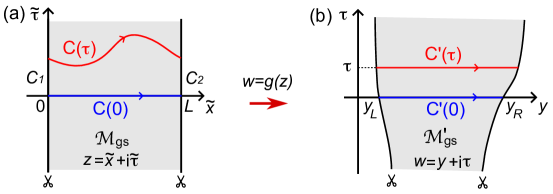
Figure S1: Illustration of the PBC Euclidean manifold $\mathcal{M}_{\text{gs}}^{\prime}$ circumference calculation in the $z$ and $w$ coordinates, respectively.

We now show that for PBC quenches with a smooth $f(x)$, the two manifolds $\mathcal{M}_{\text{gs}}^{\prime}$ and $\mathcal{M}_{\text{phy}}^{\prime}$ always match within a finite Euclidean time interval $(-\tau_{0},\tau_{0})$. This will be true if and only if $\mathcal{M}_{\text{gs}}^{\prime}$ to be a cylinder with constant circumference $y_{R}-y_{L}$ within a Euclidean time interval $(-\tau_{0},\tau_{0})$. We denote the circumference of manifold $\mathcal{M}_{\text{gs}}^{\prime}$ at a given time $\tau$ as $y_{C}(\tau)$. It can be rewritten as

$$y_{C}(\tau)=\int dy\Big{|}_{\tau}=\oint_{C^{\prime}(\tau)}dw$$ (S36)

where $C^{\prime}(\tau)$ is the closed constant $\tau$ contour shown in Fig. S1(b). Note that in Fig. S1(b), the two boundaries of the manifold $\mathcal{M}_{\text{gs}}^{\prime}$ (grey region) are images of the vertical straight lines $\tilde{x}=0$ and $\tilde{x}=L$ in $z$ coordinate (Fig. S1(a)), and the two boundaries should be understood as identified due to PBC. Assume the constant $\tau$ contour $C^{\prime}(\tau)$ in Fig. S1(b) maps back to closed contour $C(\tau)$ in Fig. S1(a) under the inverse mapping $z=g^{-1}(w)$. With $dw=\frac{dz}{f(z)}$, Eq. S36 is transformed into a contour integral in the $z$ coordinates

$$y_{C}(\tau)=\oint_{C(\tau)}\frac{dz}{f(z)}\ .$$ (S37)

Because $f(x)$ is analytical and non-negative on the real axis $x\in[0,L]$, $1/f(z)$ at least has no poles and thus zero residue within a finite range of imaginary time interval $(-\tau_{0},\tau_{0})$. Therefore, $\tau\in(-\tau_{0},\tau_{0})$, the contour integral of $1/f(z)$ along closed loop $C(0)+C_{2}-C(\tau)-C_{1}$ in Fig. S1(a) is zero, where $C(0)$ is the contour $C(\tau)$ at $\tau=0$. Note that $C_{2}$ and $C_{1}$ are identical due to PBC and cancel, and $z=x$ at time $\tau=0$, we find

$$y_{C}(\tau)=\oint_{C(\tau)}\frac{dz}{f(z)}=\oint_{C(0)}\frac{dz}{f(z)}=\int_{0}^{L}\frac{dx}{f(x)}=y_{R}-y_{L}\ .$$ (S38)

We have thus proved that PBC guarantees that $\mathcal{M}_{\text{gs}}^{\prime}$ and $\mathcal{M}_{\text{phy}}^{\prime}$ have the same constant circumference $y_{R}-y_{L}$ for all the $\tau$ within a finite Euclidean time interval $[-\tau_{0},\tau_{0}]$. In this case, the path integral reduces to a Euclidean path integral in the simple cylinder geometry $\mathcal{M}_{\text{gs}}$ in $z$ coordinate. This is similar to the simple boundary effect case of OBC quenches, which reduces to a path integral in a simple strip geometry in $z$ coordinate and leads to Eq. 13. We have thus showed that the previous solution for CFT quenches with PBC [33] always corresponds to simple Euclidean path-integral spacetime geometries, in a sense similar to the simple boundary effect for CFT quenches with OBC we identified in this paper.

.6 VI. Examples of inhomogeneous OBC quenches and a special discussion of the Möbius quench

In this section, we give calculation details and additional discussions on the quench examples we considered in main text Tab. I, and show more plots of comparison between the CFT formula and the tight-binding numerical calculations in Fig. S2.

In the main text, we have defined the light cone coordinates $x_{\pm}\in[0,L]$ as initial positions of a quasiparticle reaching point $(x,t)$ from the left/right, which we have rewritten in Eq. S19.

Once we have $y=g(x)$ for $x\in[0,L]$, for a given time $t$, we can calculate $y_{\pm}$ and $x_{\pm}$ from Eq. S19, and calculate

$$\frac{\partial x_{\pm}}{\partial x}=\frac{\partial x_{\pm}}{\partial y_{\pm}}\frac{\partial y_{\pm}}{\partial x}=\frac{f(x_{\pm})}{f(x)}\ .$$ (S39)

Then we have all the ingredients to calculate the entanglement entropy in equation Eq. 15. So we will only specify $y=g(x)$ for $x\in[0,L]$ for our quench examples shown in the main text Tab. I. The expression for $S_{A}$ comes from substituting $\frac{\partial x_{\pm}}{\partial x}$ and $x_{\pm}=g^{-1}(y_{\pm})$ in the main text Eq. 15.

1. Truncated entanglement Hamiltonian (tEH) quench. The entanglement quench is the quench associated with the deformation:

$$\begin{split}f(x)=\frac{\left(x+L_{1}\right)\left(L+L_{2}-x\right)}{L+L_{1}+L_{2}}\ ,\end{split}$$ (S40)

which yields

$$\begin{split}g(x)=\int\frac{dx}{f(x)}=\ln\left(\frac{x+L_{1}}{L+L_{2}-x}\right)\end{split}$$ (S41)

Unless $L_{1}=L_{2}=0$, the tEH quench has generic boundary effect.

Additional to the main text, Fig. S2 $(a)$ shows the free fermion numerics of tEH quench with $L_{1}=0.3L$ and $L_{2}=0$: Compared with the main text Fig. 1 $(a)$, there is only one hot spot $x_{h}=L$ in this case, and $S_{A}(x,t)$ from the CFT formula saturates at large $t$. $S_{A}(x,t)$ from tight-binding calculations deviates from the CFT formula at large $t$, as the spatial UV cutoff (lattice constant) around the hot spot prevents the saturation.

2. Truncated SRD (tSRD) quench. The tSRD quench is the quench associated with the truncated square root deformation with

$$f(x)=\sqrt{\left(x+L_{1}\right)\left(L+L_{2}-x\right)}\ .$$ (S42)

This gives

$$g(x)=\int\frac{dx}{f(x)}\quad\rightarrow\quad\frac{x+L_{1}}{L_{0}}=\frac{1-\cos g(x)}{2}\quad\rightarrow\quad g(x)=\cos^{-1}{\left(\frac{L+L_{2}-L_{1}-2x}{L+L_{1}+L_{2}}\right)}\ .$$ (S43)

The tSRD quench always has generic boundary effect.

3. The rainbow quench. The rainbow quench we consider here is the quench associated with the deformation

$$f(x)=e^{-kx}\ ,\qquad x\in[0,L]\ .$$ (S44)

Here we take $L$ finite for the purpose of comparison with the tight-binding numerical results (which can only be done for finite $L$). Taking the $L\rightarrow\infty$ limit yields the rainbow quench with $x\in[0,+\infty)$. This corresponds to

$$g(x)=\int\frac{dx}{f(x)}=\frac{e^{kx}}{k}\ .$$ (S45)

It has generic boundary effect. In thel limit $L\rightarrow\infty$, the rainbow quench always has $n_{-}=0$, and $n_{+}\leq 1$.

4. The Möbius quench. The Möbius quench is the quench associated with the deformation

$$f(x)=1-\lambda\cos\left(\frac{2\pi x}{L}\right)\ .$$ (S46)

By defining $L_{\text{eff}}=\frac{L}{\sqrt{1-\lambda^{2}}}$ and $a=\frac{\sqrt{1-\lambda^{2}}}{1+\lambda}$, one derives the relation between $x$ and $y=g(x)$:

$$y=g(x)=\int\frac{dx}{f(x)}\ ,\quad\rightarrow\quad e^{i\frac{2\pi x}{L}}=\frac{(1+a)e^{i\frac{2\pi y}{L_{\text{eff}}}}-(1-a)}{(1-a)e^{i\frac{2\pi y}{L_{\text{eff}}}}-(1+a)}\ ,$$ (S47)

From which we have

$$g(x)=\frac{L_{\text{eff }}}{\pi}\tan^{-1}\left(-\frac{a}{\tan\frac{\pi x}{L}}\right)\ .$$ (S48)

The range of $y=g(x)$ is $y\in\left[-\frac{L_{\text{eff}}}{2},\frac{L_{\text{eff}}}{2}\right]$.

The Möbius quench has simple boundary effect, which can be seen from the matching Euclidean spacetime boundaries $\partial\mathcal{M}_{\text{phy}}^{\prime}$ and $\partial\mathcal{M}_{\text{gs}}^{\prime}$ at small Euclidean time $\tau$. The boundary $\partial\mathcal{M}_{\text{phy}}^{\prime}$ is always $y=\pm L_{\text{eff}}/2$ and $\tau\in\mathbb{R}$. The boundary $\partial\mathcal{M}_{\text{gs}}^{\prime}$ is mapped via $w=g(z)$ from the straight boundaries $z=i\tilde{\tau}$ and $z=L+i\tilde{\tau}$. From Eq. S50, and using the fact that $e^{i\frac{2\pi z}{L}}=e^{-\frac{2\pi\tilde{\tau}}{L}}>0$ with $\tilde{\tau}\in\mathbb{R}$, one finds that the boundary $\partial\mathcal{M}_{\text{gs}}^{\prime}$ in coordinate $w=y+i\tau$ is located at three $y$ positions:

(1) $y=-L_{\text{eff}}/2$, $\tau\in\mathbb{R}$ .

(2) $y=L_{\text{eff}}/2$, $\tau\in\mathbb{R}$ .

(3) $y=0$, $|\tau|\geq\tau_{0}$ with $\tau_{0}=\frac{L_{\text{eff}}}{2\pi}\ln{(\frac{1+a}{1-a})}$ .

The SSD quench case is given by taking the limit $\lambda\rightarrow 1$, in which case $\tau_{0}\rightarrow\frac{L}{2\pi}$.

Therefore, the boundaries in $w$ for the Móbius quench is as shown the main text Fig. 1 $(c)$, and the two boundaries $\partial\mathcal{M}_{\text{phy}}^{\prime}$ and $\partial\mathcal{M}_{\text{gs}}^{\prime}$ match within the Euclidean time interval $\tau\in(-\tau_{0},\tau_{0})$, and simple boundary effect applies. Thus, the previous results [21, 34, 25] relying on analytical continuations agree with ours. Comparison of the entanglement entropy $S_{A}$ with the numerical tight-binding calculation for Möbius and SSD quenches are shown in Fig. S2(c)-(d), which shows analyticity at all $x\in(0,L)$. In the SSD case, $S_{A}(x,t)$ from the CFT formula is in a heating phase with perpetual linear growth in $t$, because of the two hot spots $x=0$ and $x=L$, as explained in the main text.

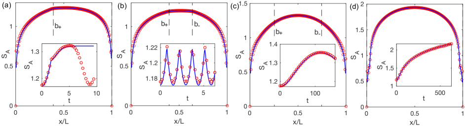
Figure S2: More numerical comparison examples between the CFT formula in main text Eq. (15) (blue lines) and the free-fermion tight-binding calculation (red circles), for system size $L=200$. Each panel shows $S_{A}(x,t_{0})$ at a fixed time $t=t_{0}$, and the inset shows $S_{A}(x_{0},t)$ at a fixed position $x=x_{0}$. The quenches and parameters are: (a) tEH with $L_{1}=0.3L$, $L_{2}=0$, $t_{0}=\frac{9\pi}{20}$, $x_{0}=0.5L$. (b) tSRD with $L_{1}=0.3L$, $L_{2}=0.2L$, $t_{0}=\frac{9\pi}{20}$, $x_{0}=0.5L$. (c) Möbius with $\lambda=0.5$, $t_{0}=25\pi$, $x_{0}=0.5L$. (d) SSD (Möbius with $\lambda=1$), $t_{0}=100\pi$, $x_{0}=0.5L$.

5. The half Möbius quench. Only in the case of half Móbius quench, which has

$$f(x)=1-\lambda\cos\left(\frac{\pi x}{L}\right),$$ (S49)

the boundaries $\partial\mathcal{M}_{\text{gs}}^{\prime}$ and $\partial\mathcal{M}_{\text{phy}}^{\prime}$ match entirely in the whole spacetime region. In this case,

$$y=g(x)=\int\frac{dx}{f(x)}\ ,\quad\rightarrow\quad e^{i\frac{\pi x}{L}}=\frac{(1+a)e^{i\frac{\pi y}{L_{\text{eff}}}}-(1-a)}{(1-a)e^{i\frac{\pi y}{L_{\text{eff}}}}-(1+a)}\ ,$$ (S50)

where $L_{\text{eff}}=\frac{L}{\sqrt{1-\lambda^{2}}}$ and $a=\frac{\sqrt{1-\lambda^{2}}}{1+\lambda}$. The boundary $\partial\mathcal{M}_{\text{phy}}^{\prime}$ is always $y=0$ and $y=L_{\text{eff}}$ with $\tau\in\mathbb{R}$. The boundary $\partial\mathcal{M}_{\text{gs}}^{\prime}$ is given by $w=g(z)$ from $z=i\tilde{\tau}$ or $z=L+i\tilde{\tau}$ with $\tilde{\tau}\in\mathbb{R}$, which correspond to $e^{i\frac{\pi z}{L}}=\pm e^{-\frac{\pi\tilde{\tau}}{L}}\in\mathbb{R}$. Therefore, $e^{i\frac{\pi w}{L_{\text{eff}}}}$ can be any real number, corresponding to the boundaries $w=i\tau$ or $L_{\text{eff}}+i\tau$ for any $\tau\in\mathbb{R}$. In this case, the boundaries match entirely, and there is no quench dynamics.

The simple boundary effect for the OBC Möbius quench and half-Möbius quench can also be understood in our ancillary mirror PBC quench problem picture as follows. The OBC Möbius quench corresponds to an ancillary mirror PBC problem with double spatial frequency Möbius quench, which can be viewed as generated by the Virasoro generators $L_{0}$ and $L_{\pm 2}$, which has nontrivial quantum dynamics. In contrast, the OBC half-Möbius quench corresponds to ancillary PBC problem of the usual Möbius quench, which can be generated by the Virasoso generators $L_{0}$ and $L_{\pm 1}$. Since $L_{0}$ and $L_{\pm 1}$ are global conformal generators and do not change the PBC ground state, quantum dynamics in this case is absent.

References

Calabrese and Cardy [2006]P. Calabrese and J. Cardy, Time dependence of
correlation functions following a quantum quench, Physical Review Letters 96, 10.1103/physrevlett.96.136801 (2006).
Kaufman et al. [2016]A. M. Kaufman, M. E. Tai,
A. Lukin, M. Rispoli, R. Schittko, P. M. Preiss, and M. Greiner, Quantum thermalization through entanglement in an isolated many-body
system, Science 353, 794 (2016).
Wen and Wu [2018a]X. Wen and J.-Q. Wu, Quantum dynamics in sine-square
deformed conformal field theory: Quench from uniform to nonuniform conformal
field theory, Physical Review
B 97, 10.1103/physrevb.97.184309
(2018a).
Goto et al. [2021]K. Goto, M. Nozaki,
K. Tamaoka, M. T. Tan, and S. Ryu, Non-equilibrating a black hole with inhomogeneous quantum quench (2021), arXiv:2112.14388
[hep-th] .
Lukin et al. [2019]A. Lukin, M. Rispoli,
R. Schittko, M. E. Tai, A. M. Kaufman, S. Choi, V. Khemani, J. Léonard, and M. Greiner, Probing entanglement in a many-body-localized system, Science 364, 256 (2019), arXiv:1805.09819 [cond-mat.quant-gas] .
Brydges et al. [2019]T. Brydges, A. Elben,
P. Jurcevic, B. Vermersch, C. Maier, B. P. Lanyon, P. Zoller, R. Blatt, and C. F. Roos, Probing
Rényi entanglement entropy via randomized measurements, Science 364, 260 (2019), arXiv:1806.05747 [quant-ph] .
Abanin and Demler [2012]D. A. Abanin and E. Demler, Measuring entanglement
entropy of a generic many-body system with a quantum switch, Phys. Rev. Lett. 109, 020504 (2012).
Alcaraz et al. [2011]F. C. Alcaraz, M. I. Berganza, and G. Sierra, Entanglement of low-energy
excitations in conformal field theory, Physical Review Letters 106, 10.1103/physrevlett.106.201601 (2011).
Islam et al. [2015]R. Islam, R. Ma, P. M. Preiss, M. E. Tai, A. Lukin, M. Rispoli, and M. Greiner, Measuring entanglement entropy in a quantum many-body system, Nature 528, 77 (2015).
Nozaki et al. [2014]M. Nozaki, T. Numasawa, and T. Takayanagi, Quantum entanglement of local
operators in conformal field theories, Physical Review Letters 112, 10.1103/physrevlett.112.111602 (2014).
Horvath et al. [2022]D. Horvath, S. Sotiriadis,
M. Kormos, and G. Takacs, Inhomogeneous quantum quenches in the sine-gordon
theory, SciPost Physics 12, 10.21468/scipostphys.12.5.144 (2022).
Capizzi and Eisler [2023]L. Capizzi and V. Eisler, Entanglement evolution
after a global quench across a conformal defect, SciPost Physics 14, 10.21468/scipostphys.14.4.070 (2023).
Christandl et al. [2004]M. Christandl, N. Datta,
A. Ekert, and A. J. Landahl, Perfect state transfer in quantum spin networks, Phys. Rev. Lett. 92, 187902 (2004).
[20]Jonah Kudler-Flam, Masahiro Nozaki, Tokiro
Numasawa, Shinsei Ryu and Mao Tian Tan, Bridging two quantum quench problems
– local joining quantum quench and Möbius quench – and their
holographic dual descriptions, to be published.
Goto et al. [2023]K. Goto, M. Nozaki,
S. Ryu, K. Tamaoka, and M. T. Tan, Scrambling and recovery of quantum information in inhomogeneous
quenches in two-dimensional conformal field theories (2023), arXiv:2302.08009
[hep-th] .
Fan et al. [2020]R. Fan, Y. Gu, A. Vishwanath, and X. Wen, Emergent spatial structure and entanglement localization
in floquet conformal field theory, Physical Review X 10, 10.1103/physrevx.10.031036
(2020).
Wen et al. [2021]X. Wen, R. Fan, A. Vishwanath, and Y. Gu, Periodically, quasiperiodically, and randomly driven
conformal field theories, Physical Review Research 3, 10.1103/physrevresearch.3.023044 (2021).
Fan et al. [2021]R. Fan, Y. Gu, A. Vishwanath, and X. Wen, Floquet conformal field theories with generally deformed
hamiltonians, SciPost
Physics 10, 10.21468/scipostphys.10.2.049 (2021).
Wen et al. [2022]X. Wen, Y. Gu, A. Vishwanath, and R. Fan, Periodically, quasi-periodically, and randomly driven
conformal field theories (II): Furstenberg's theorem and
exceptions to heating phases, SciPost Physics 13, 10.21468/scipostphys.13.4.082 (2022).
Han and Wen [2020]B. Han and X. Wen, Classification of S L2 deformed
Floquet conformal field theories, Physical Review B 102, 10.1103/physrevb.102.205125
(2020).
Lapierre et al. [2020a]B. Lapierre, K. Choo,
A. Tiwari, C. Tauber, T. Neupert, and R. Chitra, Fine structure of heating in a quasiperiodically driven critical
quantum system, Physical Review
Research 2, 10.1103/physrevresearch.2.033461 (2020a).
Lapierre et al. [2020b]B. Lapierre, K. Choo,
C. Tauber, A. Tiwari, T. Neupert, and R. Chitra, Emergent black hole dynamics in critical floquet systems, Physical Review Research 2, 10.1103/physrevresearch.2.023085 (2020b).
Moosavi [2021]P. Moosavi, Inhomogeneous conformal
field theory out of equilibrium, Annales Henri Poincaré 10.1007/s00023-021-01118-0
(2021).
Lapierre and Moosavi [2021]B. Lapierre and P. Moosavi, Geometric approach to
inhomogeneous floquet systems, Physical Review B 103, 10.1103/physrevb.103.224303
(2021).
Vitagliano et al. [2010]G. Vitagliano, A. Riera, and J. I. Latorre, Volume-law scaling for the
entanglement entropy in spin-1/2 chains, New Journal of Physics 12, 113049 (2010).
Hikihara and Nishino [2011]T. Hikihara and T. Nishino, Connecting distant ends
of one-dimensional critical systems by a sine-square deformation, Phys. Rev. B 83, 060414 (2011).
Dubail et al. [2017]J. Dubail, J.-M. Stéphan, J. Viti, and P. Calabrese, Conformal field theory
for inhomogeneous one-dimensional quantum systems: the example of
non-interacting fermi gases, SciPost Physics 2, 10.21468/scipostphys.2.1.002
(2017).
Wen et al. [2016]X. Wen, S. Ryu, and A. W. W. Ludwig, Evolution operators in conformal field
theories and conformal mappings: Entanglement hamiltonian, the sine-square
deformation, and others, Physical Review B 93, 10.1103/physrevb.93.235119
(2016).
Casini et al. [2016]H. Casini, H. Liu, and M. Mezei, Spread of entanglement and causality, Journal of High Energy Physics 2016, 10.1007/jhep07(2016)077 (2016).
Fendley et al. [2004]P. Fendley, K. Sengupta, and S. Sachdev, Competing density-wave orders in a
one-dimensional hard-boson model, Physical Review B 69, 10.1103/physrevb.69.075106
(2004).
Lesanovsky and Katsura [2012]I. Lesanovsky and H. Katsura, Interacting fibonacci
anyons in a rydberg gas, Phys. Rev. A 86, 041601 (2012).
Bernien et al. [2017]H. Bernien, S. Schwartz,
A. Keesling, H. Levine, A. Omran, H. Pichler, S. Choi, A. S. Zibrov, M. Endres, M. Greiner,
V. Vuletić, and M. D. Lukin, Probing many-body dynamics on a 51-atom quantum
simulator, Nature 551, 579 (2017).
Keesling et al. [2019]A. Keesling, A. Omran,
H. Levine, H. Bernien, H. Pichler, S. Choi, R. Samajdar, S. Schwartz,
P. Silvi, S. Sachdev, P. Zoller, M. Endres, M. Greiner, V. Vuletić, and M. D. Lukin, Quantum kibble–zurek mechanism and critical dynamics on a
programmable rydberg simulator, Nature 568, 207 (2019).
Rader and Läuchli [2019]M. Rader and A. M. Läuchli, Floating phases in
one-dimensional rydberg ising chains (2019), arXiv:1908.02068 [cond-mat.quant-gas]
.
Slagle et al. [2021]K. Slagle, D. Aasen,
H. Pichler, R. S. K. Mong, P. Fendley, X. Chen, M. Endres, and J. Alicea, Microscopic
characterization of ising conformal field theory in rydberg chains, Physical Review B 104, 10.1103/physrevb.104.235109
(2021).
Akal et al. [2022]I. Akal, T. Kawamoto,
S.-M. Ruan, T. Takayanagi, and Z. Wei, Zoo of holographic moving mirrors, Journal of High Energy Physics 2022, 10.1007/jhep08(2022)296 (2022).