Connecting NTK and NNGP: A unified theoretical framework for neural network learning dynamics in the kernel regime

Connecting NTK and NNGP:
A Unified Theoretical Framework for Neural Network Learning Dynamics in the Kernel Regime

Abstract

Artificial neural networks (ANNs) have revolutionized machine learning in recent years, but a complete theoretical framework for their learning process is still lacking. Substantial theoretical advances have been achieved for infinitely wide networks. In this regime, two disparate theoretical frameworks have been used, in which the network’s output is described using kernels: one framework is based on the Neural Tangent Kernel (NTK) which assumes linearized gradient descent dynamics, while the Neural Network Gaussian Process (NNGP) kernel assumes a Bayesian framework. However, the relation between these two frameworks and between their underlying sets of assumptions has remained elusive. This work unifies these two distinct theories using a Markov proximal learning model for learning dynamics in an ensemble of randomly initialized infinitely wide deep networks. We derive an exact analytical expression for the network input-output function during and after learning, and introduce a new time-dependent Neural Dynamical Kernel (NDK) from which both NTK and NNGP kernels can be derived. We identify two important learning phases characterized by different time scales: gradient-driven and diffusive learning. In the initial gradient-driven learning phase, the dynamics is dominated by deterministic gradient descent, and is adequately described by the NTK theory. This phase is followed by the slow diffusive learning stage, during which the network parameters sample the solution space, ultimately approaching the equilibrium posterior distribution corresponding to NNGP. Combined with numerical evaluations on synthetic and benchmark datasets, we provide novel insights into the different roles of initialization, regularization, and network depth, as well as phenomena such as early stopping and representational drift. This work closes the gap between the NTK and NNGP theories, providing a comprehensive framework for understanding the learning process of deep neural networks in the infinite width limit.

1 Introduction

Despite the empirical success of artificial neural networks (ANNs), theoretical understanding of their underlying learning process is still limited. One promising theoretical approach focuses on deep wide networks, in which the number of parameters in each layer goes to infinity whereas the number of training examples remains finite [1, 2, 3, 4, 5, 6, 7, 8, 9, 10, 11]. In this regime, the neural network (NN) is highly over-parameterized, and there is a degenerate space of solutions achieving zero training error. Investigating the properties of the solution space offers an opportunity for understanding learning in over-parametrized NNs [12, 13, 14]. The two well-studied theoretical frameworks in the infinite width limit focus on two different scenarios for exploring the solution space during learning. One considers randomly initialized NNs trained with gradient descent dynamics, and the learned NN parameters are largely dependent on their value at initialization. In this case, the infinitely wide NN’s input-output relation is captured by the neural tangent kernel (NTK) [2, 4]. The other scenario considers Bayesian neural networks (BNNs) with an i.i.d. Gaussian prior over their parameters, and a learning-induced posterior distribution. In this case, the statistics of the NN’s input-output relation in the infinite width limit are given by the neural network Gaussian process (NNGP) kernel [3, 15]. These two scenarios make different assumptions regarding the learning process and regularization. Furthermore, for some datasets the generalization performance of the two kernels differs significantly [16]. It is therefore important to generate a unified framework with a single set of priors and regularizations describing a dynamical process that captures both cases. Such a theory may also provide insight into salient dynamical phenomena such as early stopping [17, 18, 19, 20, 21]. From a neuroscience perspective, a better understanding of the exploratory process leading to Bayesian equilibrium may shed light on the empirical and hotly debated phenomenon of representational drift [22, 23, 24, 25, 26, 27, 28]. To this end, we derive a new analytical theory of the learning dynamics in infinitely wide ANNs. Our main contributions are:

1. We propose a novel Markov proximal learning framework, which generalizes Langevin gradient descent dynamics [29, 30]. The framework provides a novel application of statistical physics for analysis of the noisy gradient-based learning dynamics. We derive an analytical expression for the time evolution of the mean input-output relation (i.e. the mean predictor) of the network in the form of an integral equation, and demonstrate its remarkable agreement with computer simulations.

2. A new time-dependent kernel, the Neural Dynamical Kernel (NDK), naturally emerges from our theory and we derive explicit relations between the NDK and both the NTK and the NNGP kernels.

3. Our theory reveals two important learning phases characterized by different time scales: gradient-driven and diffusive learning. In the initial gradient-driven learning phase, the dynamics are primarily governed by deterministic gradient descent, and can be described by the NTK theory. This phase is followed by the slow diffusive stage, during which the network parameters sample the solution space, ultimately approaching the equilibrium posterior distribution corresponding to NNGP. (Another perspective on the two phases was offered [31]).

4. We apply our theory to both synthetic and benchmark datasets and present several predictions. Firstly, the generalization error may exhibit diverse behaviors during the diffusive learning phase depending on network depth and the ratio between initialization and regularization strengths. Our theory provides insights into the roles of these hyper-parameters in early stopping. Secondly, through analysis of the temporal correlation between network weights during diffusive learning, we show that despite the random diffusion of hidden layer weights, the training error remains stable at a very low value due to a continuous realignment of readout weights and network hidden layer weights. Conversely, a time delay in this alignment degrades the network performance due to decorrelation in the representation, ultimately leading to degraded performance. We derive conditions under which the performance upon completely decorrelated readout and hidden weights remain well above chance. This provides insight into the representational drift and its consequences observed in biological neuronal circuits.

2 Markov Proximal Learning (MPL) framework for learning dynamics

In this section, we first introduce our Markov proximal learning framework for learning dynamics in fully connected deep neural networks (DNNs). We formally write down the moment generating function (MGF) of the predictor. We then use the well-known replica method in statistical physics [32, 33], which has also been shown to be a powerful tool for deriving analytical results for learning in NNs [34, 35, 36, 37, 38]. We analytically calculate the MGF after averaging over the posterior distribution of the network weights in the infinite width limit, which enables us to compute statistics of the predictor.

2.1 Definition of MPL

We consider a fully connected DNN with $L$ hidden layers and a single output, with the following time-dependent input-output function:

$$f\left({\bf x},\Theta_{t}\right) =\frac{1}{\sqrt{N_{L}}}{\bf a}_{t}\cdot{\bf x}_{t}^{L},\ \ \ \ {\bf a}_{t}\in\mathbb{R}^{N}$$ (1)

$${\bf x}_{t}^{l}\left({\bf x},{\bf W}_{t}^{1},\cdots,{\bf W}_{t}^{l}\right) =\phi\left(N_{l-1}^{-1/2}{\bf W}_{t}^{l}\cdot{\bf x}_{t}^{l-1}\right),\ \ \ \ \mathbf{x}_{t}^{l}\in\mathbb{R}^{N_{l}}\ \ \ \ ,l=1,\cdots,L$$ (2)

Here $N_{l}$ denotes the number of nodes in hidden layer $l$, and $N_{0}$ is the input dimension. The set of network weights at a training time $t$ is denoted collectively as $\Theta_{t}=\left\{\mathcal{W}_{t},{\bf a}_{t}\right\}$, where ${\bf a}_{t}\in\mathbb{R}^{N}$ denotes the linear readout weights and $\mathcal{W}_{t}=\left\{{\bf W}_{t}^{1},\cdots,{\bf W}_{t}^{L}\right\}$ stands for all the hidden layer weights at time $t$, with ${\bf W}_{t}^{l}\in\mathbb{R}^{N_{l}\times N_{l-1}}$ as the hidden layer weights between layer $l-1$ and $l$. $\phi\left(N_{l-1}^{-1/2}{\bf W}_{t}^{l}\cdot{\bf x}_{t}^{l-1}\right)$ is an element-wise nonlinear function of the weighted sum of its input vector. ${\bf x}\in\mathbb{R}^{N_{0}}$ denotes the input vector to the first layer of the network (${\bf x}^{l=0}={\bf x}$). The training data is a set of $P$ labeled examples $\mathcal{D}:\left\{{\bf x}^{\mu},y^{\mu}\right\}_{\mu=1,\cdots,P}$ where ${\bf x}^{\mu}\in\mathbb{R}^{N_{0}}$ is the input vector, and $y^{\mu}$ is a scalar denoting the target label of ${\bf x}^{\mu}$. We consider the supervised learning cost function:

$$E\left(\Theta_{t}|\mathcal{D}\right)=\frac{1}{2}\sum_{\mu=1}^{P}\left(f\left({\bf x}^{\mu},\Theta_{t}\right)-y^{\mu}\right)^{2}+\frac{T}{2\sigma^{2}}\left|\Theta_{t}\right|^{2}$$ (3)

The first term is the square error empirical loss (SE loss), and the second term is a regularization term that favors weights with small $L_{2}$ norm, where $\left|\Theta_{t}\right|^{2}$ is the sum of the squares of all weights. It is convenient to introduce the temperature parameter $T$ as controlling the relative strength of the regularization, and $\sigma^{2}$ is the variance of the equilibrium distribution of the Gaussian prior.

We consider the network learning dynamics as a Markov proximal process, which is a generalized version of the deterministic proximal algorithm [39, 40]. Deterministic proximal algorithm with $L_{2}$ regularization is a sequential update rule defined as $\Theta_{t}\left(\Theta_{t-1},\mathcal{D}\right)=\arg\min_{\Theta}\left(E\left(\Theta|\mathcal{D}\right)+\frac{\lambda}{2}\left|\Theta-\Theta_{t-1}\right|^{2}\right)$ where $\lambda$ is a parameter determining the strength of the proximity constraint. This algorithm has been proven to converge to the global minimum for convex cost functions [41, 42], and many optimization algorithms widely used in machine learning can be seen as its approximations[43, 44, 45, 46]. We define a stochastic extension of proximal learning, the Markov proximal learning, through the following transition density

$$\mathcal{T}\left(\Theta_{t}|\Theta_{t-1}\right)=\frac{1}{Z\left(\Theta_{t-1}\right)}\exp\left(-\frac{1}{2}\beta\left(E\left(\Theta_{t}\right)+\frac{\lambda}{2}\left|\Theta_{t}-\Theta_{t-1}\right|^{2}\right)\right)$$ (4)

where $Z\left(\Theta_{t-1}\right)$ is the single time partition function, $Z\left(\Theta_{t-1}\right)=\intop d\Theta^{\prime}\mathcal{T}\left(\Theta^{\prime}|\Theta_{t-1}\right)$. $\beta=T^{-1}$ is an inverse temperature parameter characterizing the level of ’uncertainty’ and $\beta\rightarrow\infty$ limit recovers the deterministic proximal algorithm. We further assume that the initial distribution of $\Theta$ is an i.i.d. Gaussian with variance $\sigma_{0}^{2}$ and zero mean. Finally, we note that in the large $\lambda$ limit, the difference between $\Theta_{t}$ and $\Theta_{t-1}$ is infinitesimal, and $\Theta_{t}$ becomes a smooth function of continuous time, where the time variable is the discrete time divided by $\lambda$.

Formally, we prove that there is a complete equivalence between Markov proximal learning in the large $\lambda$ limit and a continuous time Langevin dynamics (see SI Sec.A for detailed proof).

$$\frac{d}{dt}\Theta_{t}=-\nabla_{\Theta}E\left(\Theta_{t}\right)+\eta\left(t\right)$$ (5)

where $\eta$ is a white noise $\left\langle\eta\left(t\right)\eta\left(t^{\prime}\right)^{\top}\right\rangle=2IT\delta\left(t-t^{\prime}\right),\left\langle\eta\left(t\right)\right\rangle=0$.

2.2 Moment generating function (MGF) of the predictor

The MPL defines a joint probability density on trajectories of $\Theta_{t}$, and the single time marginal probability $P\left(\Theta_{t}\right)=\prod_{\tau=0}^{t}\left[\int d\Theta_{\tau}\mathcal{T}\left(\Theta_{\tau}|\Theta_{\tau-1}\right)\right]P\left(\Theta_{0}\right)$ . Of particular interest is the statistics of the predictor $f\left({\bf x},\Theta_{t}\right)$ on an arbitrary input point ${\bf x}$. These statistics can be calculated by introducing a source $\ell$ , i.e., $\mathcal{M}_{t}\left(\ell\right)\equiv\int d\Theta_{t}P\left(\Theta_{t}\right)\exp\left(\ell f\left({\bf x},\Theta_{t}\right)\right)$.

Here we focus on the limit of large $\lambda$, which corresponds to Langevin weight dynamics, namely gradient descent w.r.t. the cost function $E$ (Eq.3) with additional white noise. In this limit, the MGF can be written in terms of two fields, $u\left(t\right)\in\mathbb{R}^{P}$ and $v\left(t\right)\in\mathbb{R}^{P}$, where $v\left(t\right)$ is a measure of the loss on the training data $\left\langle iv\left(t\right)\right\rangle=\left\langle f_{\text{train}}\left(t\right)\right\rangle-Y$ where $f_{\text{train}}\left(t\right)\equiv\left[f\left({\bf x}^{1},\Theta_{t}\right),\cdots,f\left({\bf x}^{\mu},\Theta_{t}\right)\right]^{T}\in\mathbb{R}^{P}$ is the predictor on the $P$ training examples. $u\left(t\right)$ is related to the fluctuations of the predictor. The result is

$$\mathcal{M}\left[\ell\left(t\right)\right]=\intop Dv\left(t\right)\intop Du\left(t\right)\exp\left(-S\left[v\left(t\right),u\left(t\right)\right]-Q\left[\ell\left(t\right),v\left(t\right),u\left(t\right)\right]\right)$$ (6)

$$S\left[v\left(t\right),u\left(t\right)\right] =\frac{1}{2}\intop_{0}^{\infty}dt\intop_{0}^{\infty}dt^{\prime}m\left(t,t^{\prime}\right)u^{\top}\left(t\right)K^{L}\left(t,t^{\prime}\right)u\left(t^{\prime}\right)$$ (7)

$$+\intop_{0}^{\infty}dt\left(\intop_{0}^{t}dt^{\prime}K^{d,L}\left(t,t^{\prime}\right)v\left(t^{\prime}\right)+v\left(t\right)-iY\right)^{\top}u\left(t\right)$$

$$Q\left[\ell\left(t\right),v\left(t\right),u\left(t\right)\right]= i\intop_{0}^{\infty}dt\intop_{0}^{t}dt^{\prime}\left(k^{d,L}\left(t,t^{\prime}\right)\right)^{\top}v\left(t^{\prime}\right)\ell\left(t\right)$$ (8)

$$+i\intop_{0}^{\infty}dt\intop_{0}^{\infty}dt^{\prime}m\left(t,t^{\prime}\right)\left(k^{L}\left(t,t^{\prime}\right)\right)^{\top}u\left(t^{\prime}\right)\ell\left(t\right)$$

$$-\frac{1}{2}\intop_{0}^{\infty}dt\intop_{0}^{\infty}dt^{\prime}m\left(t,t^{\prime}\right)k^{L}\left(t,t^{\prime},{\bf x},{\bf x}\right)\ell\left(t\right)\ell\left(t^{\prime}\right)$$

Thus the MGF defines a Gaussian measure on the $P$ dimensional time-dependent variables $v\left(t\right)$ and $u\left(t\right)$. $S\left[v\left(t\right),u\left(t\right)\right]$ represents the source-independent part and is related to the dynamics of the predictor on the training data, while $Q\left[\ell\left(t\right),v\left(t\right),u\left(t\right)\right]$ contains the source-dependent part and determine the dynamics of the predictor on a test point. The scalar coefficient $m\left(t,t^{\prime}\right)$ is the time-dependent auto-correlations of all the weights w.r.t. the Gaussian prior (see SI Sec.B, Eq.15). The statistics of the weights w.r.t. the Gaussian prior (denoted as $S_{0}$) are given by:

$$\left\langle\Theta_{t}\Theta_{t^{\prime}}^{\top}\right\rangle_{S_{0}}=m\left(t,t^{\prime}\right)I,\left\langle\Theta_{t}\right\rangle_{S_{0}}=0$$ (9)

$$m\left(t,t^{\prime}\right)=\sigma^{2}e^{-T\sigma^{-2}\left|t-t^{\prime}\right|}+\left(\sigma_{0}^{2}-\sigma^{2}\right)e^{-T\sigma^{-2}\left(t+t^{\prime}\right)}$$ (10)

Here $T$ is the level of noise in the Langevin dynamics, $\sigma^{2}$ and $\sigma_{0}^{2}$ are the variances of the $L_{2}$ regularizer and initial weight distribution, respectively. Note that all times (here and in Eq.6) are in units of $\lambda$. As expected, $m\left(0,0\right)=\sigma_{0}^{2}$. At long times, the last (transient) term vanishes and the dominant term is the $\sigma^{2}e^{-T\sigma^{-2}\left|t-t^{\prime}\right|}$. The remaining coefficients of the MGF are various two-time kernels defined in the next section.

3 The Neural Dynamical Kernel (NDK)

In Eq.6, we introduce a new kernel, the Neural Dynamical Kernel (NDK), which can be considered as a time-dependent generalization of the NTK [2]. The kernel can be expressed in terms of the derivatives of the predictor w.r.t. the time-dependent network parameters

$$K^{d,L}\left(t,t^{\prime},{\bf x},{\bf x}^{\prime}\right)=e^{-T\sigma^{-2}\left|t-t^{\prime}\right|}\left\langle\nabla_{\Theta_{t}}f\left({\bf x},\Theta_{t}\right)\cdot\nabla_{\Theta_{t^{\prime}}}f\left({\bf x}^{\prime},\Theta_{t^{\prime}}\right)\right\rangle_{S_{0}}$$ (11)

From Eq.11 follows that at initialization $K^{d,L}\left(0,0,{\bf x},{\bf x}^{\prime}\right)=\left\langle\nabla_{\Theta_{0}}f\left({\bf x},\Theta_{0}\right)\cdot\nabla_{\Theta}f\left({\bf x^{\prime}},\Theta_{0}\right)\right\rangle_{\Theta_{0}}=K_{NTK}^{L}$ equals the NTK as the average is only over the i.i.d. Gaussian initialization. Furthermore, as we will see below, the NNGP kernel can also be evaluated from the NDK (see Sec.4.2).

The NDK can also be obtained recursively, in terms of two-time extensions of the usual NNGP kernel $K^{L}\left(t,t^{\prime},{\bf x},{\bf x}^{\prime}\right)$ and the derivative kernel $\dot{K}^{L}\left(t,t^{\prime},{\bf x},{\bf x}^{\prime}\right)$ (see SI 3 for a detailed proof of the equivalence).

$$K^{d,L}\left(t,t^{\prime},{\bf x},{\bf x}^{\prime}\right)= m\left(t,t^{\prime}\right)\dot{K}^{L}\left(t,t^{\prime},{\bf x},{\bf x}^{\prime}\right)K^{d,L-1}\left(t,t^{\prime},{\bf x},{\bf x}^{\prime}\right)$$ (12)

$$+e^{-T\sigma^{-2}\left|t-t^{\prime}\right|}K^{L}\left(t,t^{\prime},{\bf x},{\bf x}^{\prime}\right)$$

$$K^{d,L=0}\left(t,t^{\prime},{\bf x},{\bf x}^{\prime}\right)=e^{-T\sigma^{-2}\left|t-t^{\prime}\right|}\left(\frac{1}{N_{0}}{\bf x}\cdot{\bf x}^{\prime}\right)$$ (13)

The kernel $K^{L}\left(t,t^{\prime},{\bf x},{\bf x}^{\prime}\right)$ in Eqs.7,8,12 is defined as

$$K^{L}\left(t,t^{\prime},{\bf x},{\bf x}^{\prime}\right)=\frac{1}{N_{L}}\left\langle{\bf x}_{t}^{L}\left({\bf x},\mathcal{W}_{t}\right)\cdot{\bf x}_{t^{\prime}}^{L}\left({\bf x}^{\prime},\mathcal{W}_{t^{\prime}}\right)\right\rangle_{S_{0}}$$ (14)

where $N_{L}$ is the width of the $L-$ th layer and the average is w.r.t. to the prior statistics (Eq.9). The derivative kernel, $\dot{K}^{L}\left(t,t^{\prime},{\bf x},{\bf x}^{\prime}\right)$ is the kernel evaluated w.r.t. the derivative of the activation function

$$\dot{K}^{L}\left(t,t^{\prime},{\bf x},{\bf x}^{\prime}\right)=\frac{1}{N_{L}}\left\langle\dot{{\bf x}}_{t}^{L}\left({\bf x},\mathcal{W}_{t}\right)\cdot\dot{{\bf x}}_{t^{\prime}}^{L}\left({\bf x}^{\prime},\mathcal{W}_{t^{\prime}}\right)\right\rangle_{S_{0}}$$ (15)

Where $\dot{{\bf x}}^{L}\left({\bf x},\mathcal{W}_{t}\right)=\phi^{\prime}\left(N_{L-1}^{-\frac{1}{2}}{\bf W}_{t}^{L}\cdot{\bf x}_{t}^{L-1}\right)$, is the neurons activity evaluated w.r.t. the derivative of the activation function. In Eqs.7,8, $k^{d,L}\left(t,t^{\prime},{\bf x}\right)\in\mathbb{R}^{P}$ and $K^{d,L}\left(t,t^{\prime}\right)\in\mathbb{R}^{P\times P}$ are defined as applying the kernel function on the test and the training data, respectively, with $k_{\mu}^{d,L}\left(t,t^{\prime},{\bf x}\right)=K^{d,L}\left(t,t^{\prime},{\bf x},{\bf x}^{\mu}\right)$ and $K_{\mu\nu}^{d,L}\left(t,t^{\prime}\right)=K^{d,L}\left(t,t^{\prime},{\bf x}^{\mu},{\bf x}^{\nu}\right)$ and similarly for $K^{L}$. All the kernel functions above including the NDK have a closed-form expression for some nonlinearities such as ReLU and error function, as well as linear activation (see SI Sec.C,[15, 10]).

The mean predictor:The above explicit expression for the MGF allows for the evaluation of the statistics of the predictor by differentiating the MGF w.r.t. to the source $\ell$. Here we focus on its mean. The mean predictor on the training inputs obeys the following integral equation

$$\left\langle f_{\text{train}}\left(t\right)\right\rangle=\intop_{0}^{t}dt^{\prime}K^{d,L}\left(t,t^{\prime}\right)\left(Y-\left\langle f_{\text{train}}\left(t^{\prime}\right)\right\rangle\right)$$ (16)

and the mean predictor on any test point ${\bf x}$ is given by an integral over the training predictor with the NDK of the test

$$\left\langle f\left({\bf x},\Theta_{t}\right)\right\rangle=\intop_{0}^{t}dt^{\prime}\left(k^{d,L}\left(t,t^{\prime},{\bf x}\right)\right)^{\top}\left(Y-\left\langle f_{\text{train}}\left(t^{\prime}\right)\right\rangle\right)$$ (17)

4 Dynamics of the mean predictor at low $T$

We study the above equations for the mean predictor dynamics in the important limit of low $T$. As we show below, in that limit the network dynamics exhibits two distinct regimes. First, the network converges to weights with almost zero training error (error of $\mathcal{O}\left(T\right)$ ). Subsequently, the network executes slow explorations (on a time scale of $\mathcal{O}\left(T^{-1}\right)$) of the solution space. We investigate how the different parameters such as initialization, regularization and the level of noise affect the learning behavior by evaluating numerically Eqs. 16, 17.

4.1 Gradient-driven phase corresponds to NTK dynamics

The time dependence of the NDK (Eq.12) comes from exponents that scale as $T\cdot t$ (Eqs.10,12), and thus at low $T$ and $t\sim\mathcal{O}\left(1\right)$ we can substitute $K^{d,L}\left(t,t^{\prime},{\bf x},{\bf x}^{\prime}\right)=K^{d,L}\left(0,0,{\bf x}\text{,}{\bf x}^{\prime}\right)$. With Eq.11, we obtain an exact equivalence between the NDK at time zero and the NTK. In this regime, the integral equation can be transformed into a linear ODE, and solved analytically, leading to $f_{\text{train}}\left(t\right)=\left(I-\exp\left(-K_{NTK}^{L}t\right)\right)Y$, and to the well-known mean predictor in the NTK theory:

$$\left\langle f\left({\bf x},\Theta_{t}\right)\right\rangle\approx\left(k_{NTK}^{L}\left({\bf x}\right)\right)^{\top}\left[K_{NTK}^{L}\right]^{-1}\left(I-\exp\left(-K_{NTK}^{L}t\right)\right)Y,t\sim\mathcal{O}\left(1\right)$$ (18)

where we define $k_{NTK}^{L}\left({\bf x}\right)\in\mathbb{R}^{P}$ and $K_{NTK}^{L}\in\mathbb{R}^{P\times P}$ as the NTK applied on test and training data, respectively, similar to Sec.3. Thus the role of the NTK solution is made clear - it describes the dynamics of the system when the time is short compared to the level of noise in the system, such that the dynamics is approximately deterministic. Taking the large $t$ limit of the NTK dynamics (Eq.18) results in the “NTK equilibrium”, where $\left\langle f\left({\bf x},\Theta\right)\right\rangle=k_{NTK}^{L}\left({\bf x}\right)\left[K_{NTK}^{L}\right]^{-1}Y$. This short time equilibrium marks the crossover between the gradient driven phase and the diffusive learning phase. After the NTK equilibrium point, the gradient of the loss is $\mathcal{O}\left(T\right)$, and thus the two parts of the cost function Eq.3 (the SE loss and the regularization) are on equal footing, and give rise to the diffusive dynamics in time scales of $t\sim\mathcal{O}\left(T^{-1}\right)$.

4.2 Long time equilibrium corresponds to NNGP

Now we investigate the behavior at long time scales defined by $t,t^{\prime}\gg T^{-1}$ but $t-t^{\prime}=\mathcal{O}\left(T^{-1}\right)$. In this regime, $K^{d,L}\left(t,t^{\prime},{\bf x},{\bf x}^{\prime}\right)=K^{d,L}\left(t-t^{\prime},{\bf x},{\bf x}^{\prime}\right)$ is a function of the time difference through $e^{-T\sigma^{-2}\left|t-t^{\prime}\right|}$ and the transient dependence on the initialization parameter $\sigma_{0}$ vanishes. Furthermore, in this regime the NDK satisfies the following relation (see SI Sec.C.4 for detailed proof):

$$\intop_{0}^{t}K^{d,L}\left(t-t^{\prime},{\bf x},{\bf x}^{\prime}\right)dt^{\prime}=\frac{\sigma^{2}}{T}K_{GP}^{L}\left({\bf x},{\bf x}^{\prime}\right)$$ (19)

where $K_{GP}^{L}\left(\text{{\bf x}},{\bf x}^{\prime}\right)=N_{L}^{-1}\left\langle{\bf x}^{L}\left({\bf x},W\right)\cdot{\bf x}^{L}\left({\bf x}^{\prime},W\right)\right\rangle{}_{W\sim\mathcal{N}(0,\sigma^{2}I)}$ is the well-known NNGP kernel. In the long time regime defined above, $f_{\text{train}}\left(t\right)$ reaches an equilibrium state,
$f_{\text{train}}=K_{GP}^{L}\left(IT\sigma^{-2}+K_{GP}^{L}\right)^{-1}Y$ (where we define again $K_{GP}^{L}\in\mathbb{R}^{P\times P}$ as the NNGP kernel function applied to the training data). This is consistent with our assumption that the training error at long times is $\mathcal{O}\left(T\right)$. For the predictor on a test point we get

$$\lim_{t\rightarrow\infty}\left\langle f\left({\bf x},\Theta_{t}\right)\right\rangle=\left(k_{GP}^{L}\left({\bf x}\right)\right)^{\top}\left(IT\sigma^{-2}+K_{GP}^{L}\right)^{-1}Y$$ (20)

where $k_{GP}^{L}\in\mathbb{R}^{P}$ is the NNGP kernel function applied to the test data. This is the well-known equilibrium NNGP result [3]. We emphasize that this result is true for any temperature, while the NTK solution in Sec.4.1 is relevant at low $T$ only.

Our theory thus establishes the connection between the NTK and NNGP equilibria.

4.3 Time scales of the dynamics

In this section, we further examine how the time scales of the dynamics in the two phases are affected by the different hyper-parameters by numerically evaluating Eq.$\text{\ref{eq:meanftrain}},\ref{eq:meanf}$. We focus on the level of stochasticity $T$, the initialization ($\sigma_{0}^{2}$), and regularization $(\sigma^{2})$. As can be seen in Eqs.$\text{\ref{eq:mtt'}},\ref{eq:kD}$, the dynamics depend on $t$ through exponents $\exp\left(T\sigma^{-2}t\right)$ and a scalar factor that depends on $\sigma_{0}^{2}/\sigma^{2}$. To determine the time scales of the dynamics, we fix the scalar factor $\sigma_{0}^{2}/\sigma^{2}$ as a constant as we vary $\sigma_{0}^{2},\sigma^{2}$ and $T$ respectively. We consider $\sigma_{0}^{2},\sigma^{2}\sim\mathcal{O}\left(1\right)$.

First, we evaluate how the dynamics depend on the level of stochasticity determined by a small but nonzero $T$. As we see in Fig.1 (a), while the initial learning phase is not affected by $T$ since the dynamics are mainly driven by deterministic gradient descent, the diffusive phase is slower for smaller $T$ since it is driven by noise. We then investigate how the dynamics depends on $\sigma^{2}$ and $\sigma_{0}^{2}$ while fixing the ratio between them. Fig.1 (b) shows that as we increase $\sigma^{2}$ and $\sigma_{0}^{2}$ simultaneously, the gradient dynamics becomes faster since the initialization weights determined by $\sigma_{0}^{2}$ are closer to the typical solution space (with the $L_{2}$ regularization), while the dynamics of the diffusive phase becomes slower since the regularization determined by $\sigma^{2}$ imposes less constraint on the solution space, hence exploration time increases.

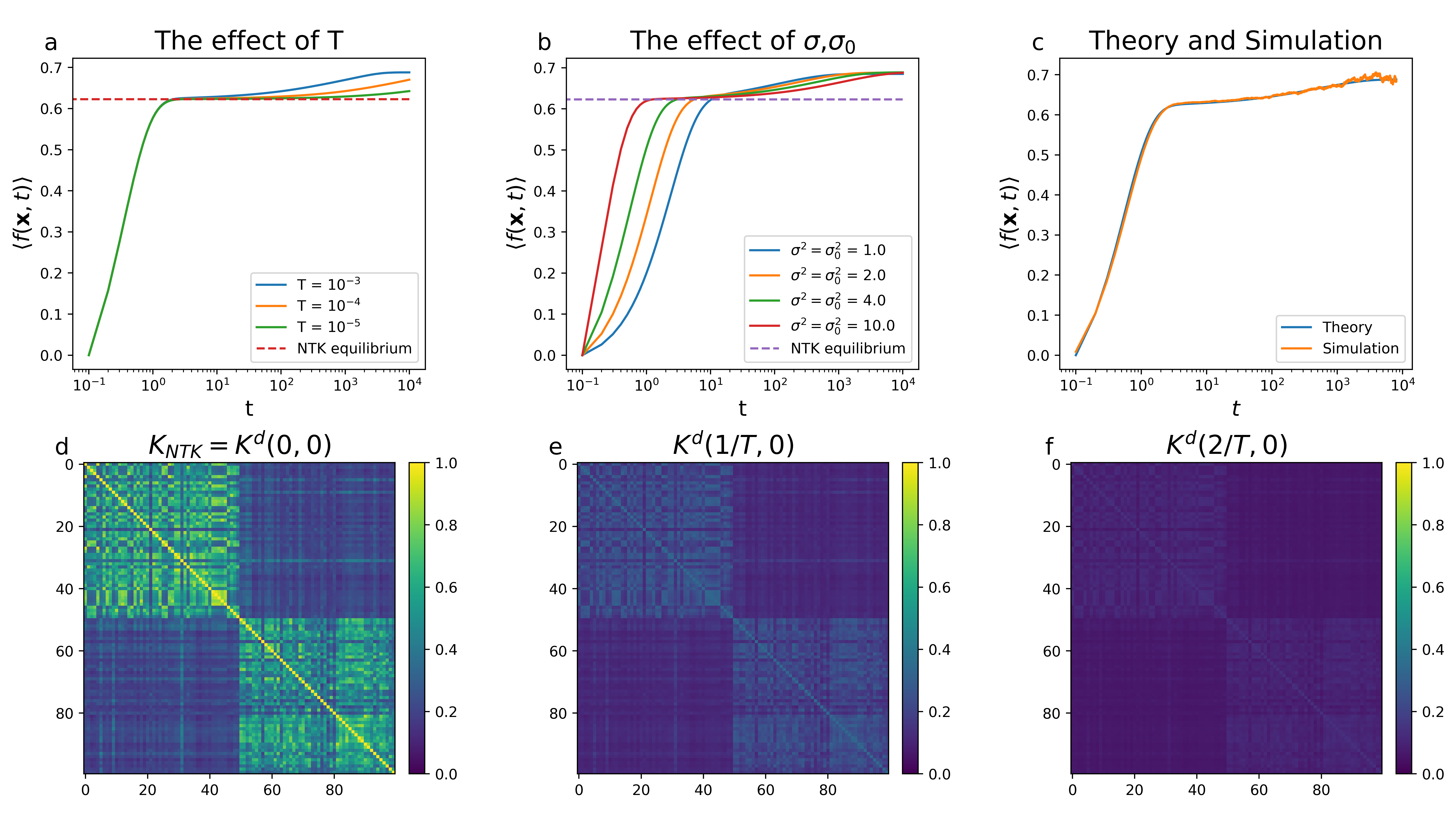
Figure 1: Time scales of the dynamics. Example using a synthetic dataset where the training inputs are orthogonal to each other with random binary labels $Y^{\mu}\in\left\{\pm 1\right\}$. Each test point has partial overlap with one input point and is orthogonal to all the others. The desired test label is the same as the label on the training input with which it has nonzero overlap. For (a-b) we plot the network mean predictor on a test point with the desired label $+1$ (see details in SI Sec.E). (a) $T$ does not affect the initial gradient-driven phase, but decreasing $T$ slows the dynamics of the diffusive learning phase. The diverging point between different T is the NTK equilibrium (b) Increasing $\sigma^{2}$ and $\sigma_{0}^{2}$ simultaneously (keeping $\sigma^{2}=\sigma_{0}^{2}$) affects the time scales of the two phases differently. The time scale of the gradient-driven phase decreases as $\sigma_{0}^{2}$ increases and vice versa in the diffusive dynamics. (c) The mean predictor calculated by Langevin simulations of neural networks for the synthetic dataset agrees well with the theory prediction. (d-f) The NDK for MNIST binary classification of the digits 0,1 [47]. The kernel vanishes as $\left(t-t^{\prime}\right)\cdot T$ increases, due to the random drift of the weights.

4.4 Diffusive learning dynamics exhibit diverse behaviors

In this section, we focus on the diffusive phase, where $t\sim\mathcal{O}\left(1/T\right)$. Unlike the simple exponential relaxation of the gradient descent regime, in the diffusive phase, the predictor dynamics exhibit complex behavior dependent on depth, regularization, initialization and the data. We systematically explore these behaviors by solving the integral equations (Eqs.$\text{\ref{eq:meanftrain}},\ref{eq:meanf}$) numerically for benchmark data sets as well as a simplified synthetic task (see details of the tasks in Fig.1,2 captions and SI Sec.E). We verify the theoretical predictions with simulations of the gradient-based Langevin dynamics of finite width neural networks, as shown in Fig.1(c) and SI Sec.F . Even though in the diffusive phase, the dominant dynamics is driven by noise and the regularization, the learning signal (both on the readout weights and the hidden layers) from the gradient of the loss is what restricts the exploration to the subspace of zero ($\mathcal{O}(T)$) training error, and without it the performance will deteriorate back to chance.

The role of initialization and regularization and early stopping phenomena: We investigate how the diffusive dynamics is affected by the $\sigma_{0}^{2}$ for fixed values of $\sigma^{2}$ and $T$ (thus fixing the time scale of the diffusive learning phase). As expected, the training predictor converges fast to the desired value and exhibits little deviation afterward (see Fig.2 (a)). In the previous section, we kept the ratio $\sigma_{0}^{2}/\sigma^{2}$ fixed, resulting in the same qualitative behavior with different time scales. In Fig.2(b-d) , we show that changing the ratio $\sigma_{0}^{2}/\sigma^{2}$ results in qualitatively different behaviors of the trajectory, shown across network depth and nonlinearities. (In the following, unless otherwise stated, we will refer to the test-predictor simply as the predictor). Interestingly, in most examples, when $\sigma_{0}^{2}/\sigma^{2}$ is small, the predictor dynamics is non-monotoinc, overshooting above its equilibrium value. The optimal early stopping point, defined as the time the network reaches the optimum generalization error occurs in some cases in the diffusive learning phase, as shown in Fig.2(b,c). In these cases, the performance in the diffusive phase is better than both equilibria. We study the effect of $\sigma_{0}^{2}/\sigma^{2}$ on the early stopping point systematically in the synthetic dataset in Fig.3.

The role of depth: The effect of different $\sigma_{0}^{2}/\sigma^{2}$ ratios on the dynamics increases with depth, resulting in distinctively different behavior for different ratios. Depth also changes the NTK and NNGP equilibrium, typically in favor of the NNGP solution as the network grows deeper (see SI Sec.D.1). Furthermore, as shown in Fig.3, depth also has an effect on the occurrence of the optimal early stopping time. In the synthetic dataset, the early stopping time occurs earlier in shallower networks for small $\sigma_{0}^{2}/\sigma^{2}$, and does not occur when $L>3$.

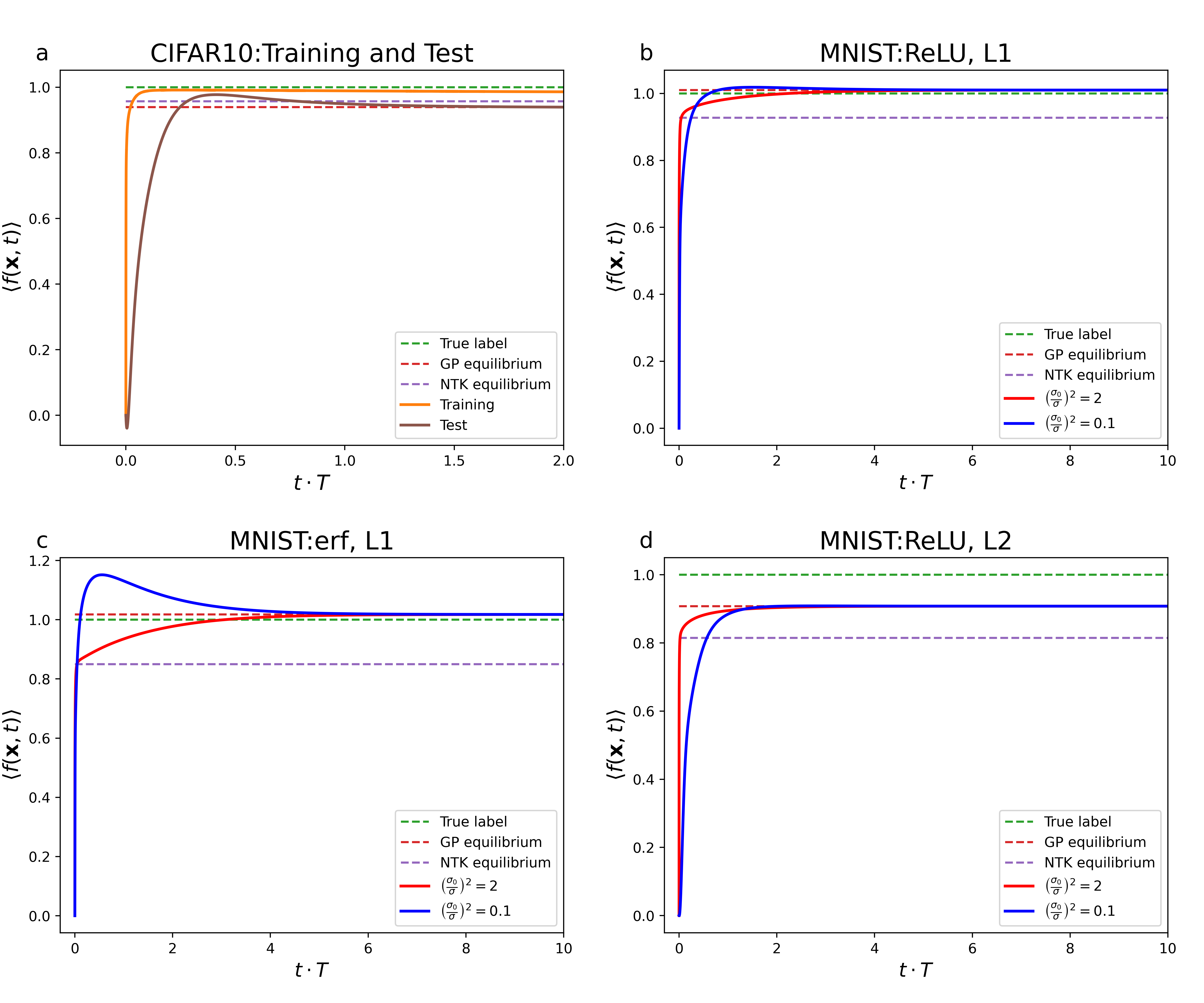
Figure 2: Dynamics of the mean predictor on a given test point in benchmark datasets. All test points shown have a target label $+1$. (a) Result on CIFAR10 dataset [48] with binary classification of cats vs dogs, for $\sigma_{0}^{2}/\sigma^{2}=2$. We see a fast convergence of the mean predictor on the training point while the test point exhibits diffusive learning phase on time scales $t\sim\mathcal{O}\left(1/T\right)$. (b-d) Results on MNIST dataset with binary classification of 0 vs 1 digits, for $L=1,2$. In $L=2$ the effect of $\sigma_{0}^{2}/\sigma^{2}$ is larger. (d) Results on MNIST dataset in a network with an error function (erf) nonlinearity with a single hidden layer. The effect $\sigma_{0}^{2}/\sigma^{2}$ is significantly larger than in (b,c).

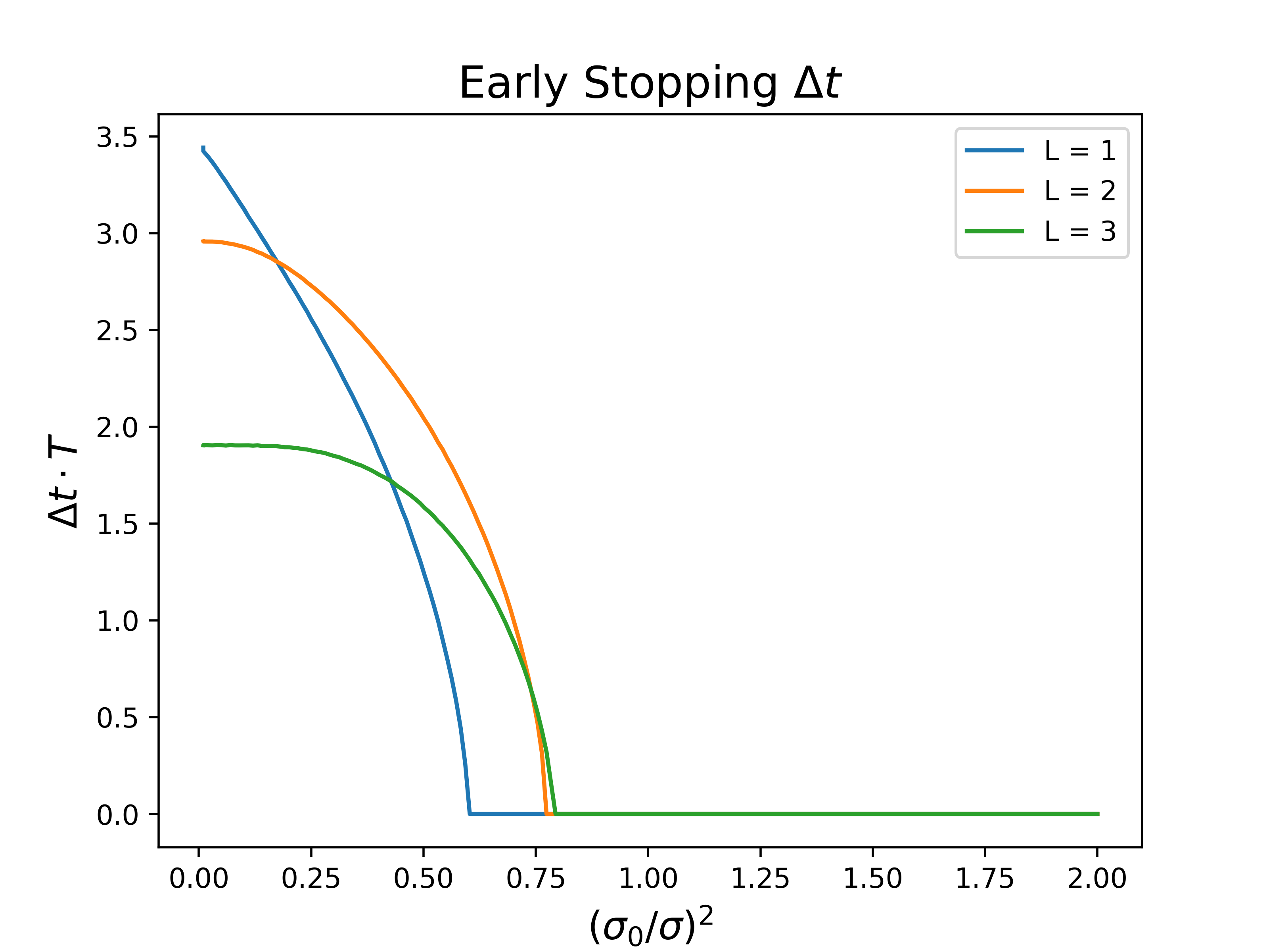
Figure 3: The optimal early stopping time for the synthetic orthogonal dataset in networks with hidden layers $L=1,2,3$. We present the time difference between the optimal stopping time and the long-time equilibrium time scaled by $T$ (denoted by $\Delta t\cdot T$). We see that for small $\sigma_{0}^{2}/\sigma^{2}$ the optimal stopping time occurs during the diffusive learning phase, while for large $\sigma_{0}^{2}/\sigma^{2}$ the optimal stopping time is only at the long time equilibrium corresponds to NNGP. Interestingly, in this dataset for $L>3$ there is no early stopping point.

The role of nonlinearity: We compare the behaviors of networks with ReLU and error function, with both having closed-form expression for their NDK (see SI C). As shown in Fig.2(c) with error function nonlinearity, the difference between NTK and NNGP is larger and the effect of $\sigma_{0}^{2}/\sigma^{2}$ on the network dynamics is more significant.

5 Representational drift during diffusive synaptic dynamics

We now explore the implications of the diffusive learning dynamics on the phenomenon of representational drift. Representational drift refers to neuroscience observations of neuronal activity patterns accumulating random changes over time without noticeable consequences on the relevant animal behavior. These observations raise fundamental questions about the causal relation between neuronal representations and the underlying computation. Some of these observations were in the context of learned behaviors and learning-induced changes in neuronal activity. One suggestion has been that the representational drifts are compensated by changes in the readout of the circuit, leaving intact its input-output relation [49, 50, 28]. We provide a general theoretical framework for studying such dynamics. In our model, the stability of the (low) training error during the diffusion phase, is due to the continuous realignment of readout weights ${\bf a}_{t}$ to changes in the network hidden layer weights $\mathcal{W}_{t}$ as they drift simultaneously exploring the space of solutions.

The above alignment scenario requires an ongoing learning signal acting on the weights. To highlight the importance of this signal, we consider an alternative scenario where the readout weights are frozen at some time (denoted as $t_{0}$) after achieving low training error while the weights of the hidden layers $\mathcal{W}_{t}$ continue to drift randomly without an external learning signal. We will denote the output of the network in this scenario as $f_{\text{drift}}\left({\bf x},t,t_{0}\right)$. Our formalism allows for computation of the mean of $f_{\text{drift}}\left({\bf x},t,t_{0}\right)$ (see SI Sec.D for details). We present here the results for large $t_{0}$, i.e. after the learning has finished.

$$\left\langle f_{\text{drift}}\left({\bf x},t-t_{0}\right)\right\rangle=\left(k^{L}\left({\bf x},t-t_{0}\right)\right)^{\top}\left(IT\sigma^{-2}+K_{GP}^{L}\right)^{-1}Y$$ (21)

The kernel $k^{L}({\bf x},t-t_{0})$ represents the overlap between the representations of the training inputs at time $t_{0}$ and that of a test point at time $t$ . When $t-t_{0}$ is large, the two representations completely decorrelate and the predictor is determined by a new kernel $K_{mean}^{L}\left({\bf x},{\bf x}^{\prime}\right)$defined as

$$K_{mean}^{L}\left({\bf x},{\bf x}^{\prime}\right)=\frac{1}{N_{L}}\left\langle{\bf x}^{L}\left({\bf x},\mathcal{W}\right)\right\rangle_{\mathcal{W}\sim\mathcal{N}\left(0,I\sigma^{2}\right)}\cdot\left\langle{\bf x}^{L}\left({\bf x}^{\prime},\mathcal{W}\right)\right\rangle_{\mathcal{W}\sim\mathcal{N}\left(0,I\sigma^{2}\right)}$$ (22)

which is a modified version of the NNGP kernel where the Gaussian averages are performed separately for each data point.

$$\lim_{t-t_{0}\rightarrow\infty}\left\langle f_{\text{drift}}\left({\bf x},t-t_{0}\right)\right\rangle\rightarrow\left(k_{mean}^{L}\left({\bf x}\right)\right)^{\top}\left(IT\sigma^{-2}+K_{GP}^{L}\right)^{-1}Y$$ (23)

where $k_{mean}^{L}\left({\bf x}\right)$ is defined as applying the mean kernel function to the test data.

For some nonlinearities (e.g. linear and error function activation) $K_{mean}^{L}\left({\bf x},{\bf x}^{\prime}\right)$ is identically zero. This however, is not the case for other nonlinearities (e.g. ReLU). In these cases its value depends on the input vectors’ norms $\left\|{\bf x}\right\|,\left\|{\bf x}^{\prime}\right\|$. Thus, if the distribution of the norms is informative of the given task, the predictor can still be useful despite the drift process. In this case, we can say that the norms are drift-invariant information. In other cases, the norms may not be relevant to the task, in which case the decorrelated output will yield a chance-level performance.

We present examples for both scenarios in Fig.4. We consider two MNIST binary classification tasks, after reaching the long time equilibrium. For each one we show the evolution of the histograms of the predictor on the training examples at times $t$, after freezing readout weights at an earlier time $t_{0}$. We train a linear classifier on top of the training predictors to evaluate the classification accuracy (see SI Sec.D for details). In the case of the classification task of the digit pair 4,9, the two histograms eventually overlap each other, resulting in a long time chance level accuracy and a complete loss of the learned information. In contrast, in the classification of the digit pair 0,1 (Fig.4(f-j)), the histogram of the two classes are partially separated, leading to a long time accuracy of 90%, reflecting the residual information in the input norms. Interestingly during the dynamics from the original state to the long time state the distributions cross each other, resulting in a short period of chance performance.

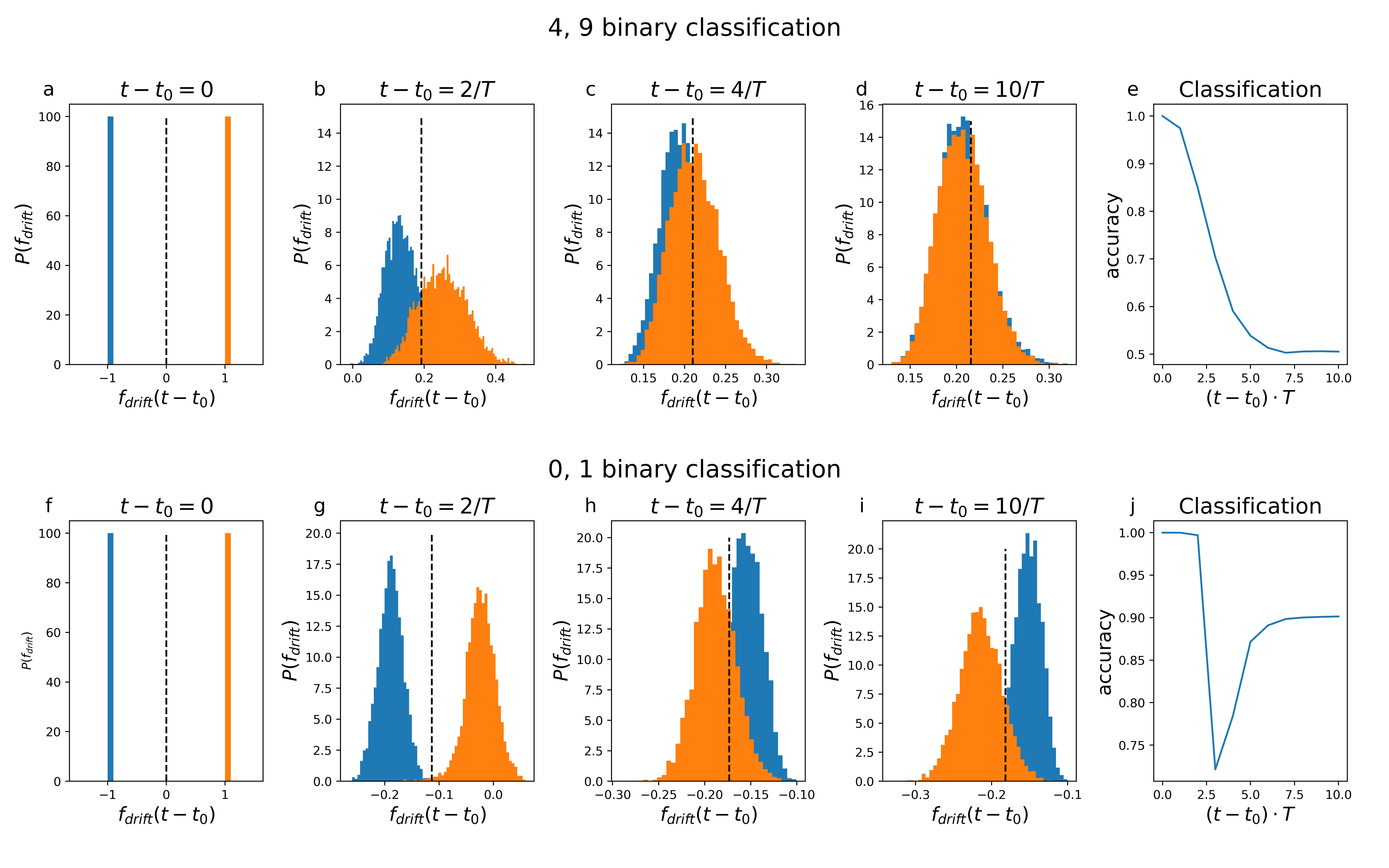
Figure 4: Representational drift with ${\bf a}_{t_{0}}$ fixed at a long time equilibrium $t_{0}$. (a-d,f-i) The dynamics of the probability distribution of $f_{\text{drift}}\left({\bf x},t-t_{0}\right)$ on the training data, starting with two delta functions at $\pm 1$, and gradually decays in performance when ${\bf a}_{t_{0}}$ and $\mathcal{W}_{t}$ lose alignment. On classification between the digits 0, 1, the norm of the images has enough information to classify them with reasonable success even after complete decorrelation, while on classification between the digits 4,9 the performance is reduced to chance. (e,j) The performance as a function of the time difference from the freezing point $t_{0}$.

6 Discussion

Our work provides the first theoretical understanding of the complete trajectory of gradient descent learning dynamics of wide DNNs in the presence of small noise, unifying the NTK theory and the NNGP theory as two limits of the same underlying process. While the noise is externally injected in our setup, stochasticity in the machine learning context may arise from randomness in the data in stochastic gradient descent, making noisy gradient descent a relevant setting in reality [51, 52, 53, 54]. We derive a new kernel, the time-dependent NDK , and show that it can be interpreted as a dynamic generalization of the NTK, and provide new insights into learning dynamics in the diffusive learning phase as the learning process explores the solution space. We focus on two particularly interesting phenomena of early stopping and representational drift. We identify an important parameter $\sigma_{0}^{2}/\sigma^{2}$ characterizing the relative weight amplitude induced by initialization and Bayesian prior regularization, which plays an important role in shaping the trajectories of the predictor.

In most of our examples, the best performance is achieved after the gradient-driven learning phase, indicating that exploring the solution space improves the network’s performance, consistent with empirical findings [16]. For some examples, the optimal stopping point occurs during the diffusive phase, before the long-time equilibrium. We stress that our ‘early stopping’ is ‘early’ compared to the NNGP equilibrium, and is different from the usual notion of early stopping, which happens in the gradient-driven learning phase [20, 2, 21]. Our theory provides insights into how and when an early stopping point can happen after the network reaches an essentially zero training error.

Our Bayesian framework provides a model of representational drift where the hidden layer weights undergo random drifts, while the readout weights is continuously realigning to keep performance unchanged, as previously suggested [49, 50]. In our framework, this realignment is due to the presence of a loss-gradient signal. The source of the putative realignment signals in brain circuits is unclear. An alternative hypothesis is that computations in the neuronal circuits are based on features that are invariant to the representational drift [22, 26, 23, 55, 56, 57]. We provide an example of such features and show that performance can be maintained after drift.

We provide a general framework of Markov proximal learning, enabling the application of tools from statistical physics for the analysis of the learning dynamics. The framework bears similarities to the Franz-Parisi potential in spin glasses [58]. A similar approach has also been used by [59] for curriculum sequential learning of two tasks in single-layer perceptrons for a teacher-student task. Our framework is more general as it goes beyond two steps and considers learning in DNNs on arbitrary datasets. Another common treatment of learning dynamics analysis in statistical mechanics is the dynamical mean field theory (DMFT) [60, 61, 53]. Importantly, our framework is more general than continuous time gradient dynamics and can be readily extended to discrete dynamics with finite and time-dependent $\lambda$ (corresponding to large step size and adaptive learning rate) and non-smooth optimization problems (potentially due to non-smooth activation functions or regularizers) [39, 62, 41] which can not be captured by DMFT. These possibilities are being explored as part of our ongoing research.

So far we have focused on learning in infinitely wide networks in the lazy regime, where the time dependence of the NDK results from random drift in the solution space. Empirical time-dependent NTK is more complex due to feature learning exist in finite width NNs [63, 64, 65] or in infinite width network with non-lazy regularization [60]. Future work on the Markov proximal learning framework aims to extend the theory to the regime where data size is proportional to network width where we expect dynamic kernel renormalization [66, 67] and to the dynamics of feature learning in non-lazy regularization [68, 69, 70].

Acknowledgments: We thank the anonymous reviewers for their helpful comments. This research is supported by the Gatsby Charitable Foundation, the Swartz Foundation, and ONR grant No.N0014-23-1-2051.

Supplemental Information

Appendix A Markov proximal learning and the Langevin dynamics

In this chapter, we prove the equivalence between Markov proximal learning and Langevin dynamics in the large $\lambda$ (continuous time) limit.

Markov proximal learning:

A deterministic proximal learning algorithm is defined as:

$$\Theta_{t}\left(\Theta_{t-1},\mathcal{D}\right)=\arg\min_{\Theta}\left(E\left(\Theta|\mathcal{D}\right)+\frac{\lambda}{2}\left|\Theta-\Theta_{t-1}\right|^{2}\right)$$ (1)

As introduced in section 2.1 in the main text, we generalize this algorithm by defining a Markov proximal learning through the transition density

$$P\left(\Theta_{t}\right)=\intop d\Theta_{t-1}\mathcal{T}\left(\Theta_{t}|\Theta_{t-1}\right)P\left(\Theta_{t-1}\right)$$ (2)

$$\mathcal{T}\left(\Theta_{t}|\Theta_{t-1}\right)=\frac{1}{Z\left(\Theta_{t-1}\right)}\exp\left(-\frac{1}{2}\beta\left(E\left(\Theta_{t}\right)+\frac{\lambda}{2}\left|\Theta_{t}-\Theta_{t-1}\right|^{2}\right)\right)$$ (3)

where $Z\left(\Theta_{t-1}\right)=\intop d\Theta^{\prime}\mathcal{T}\left(\Theta^{\prime}|\Theta_{t-1}\right)$ ensures proper normalization of $\mathcal{T}$. With this transition density we can compute the probability of a sequence $(\Theta_{0},\Theta_{1},...,\Theta_{t}).$

$$P\left(\Theta_{0},\Theta_{1},...,\Theta_{t}\right)=\left[\prod_{\tau=1}^{t}\mathcal{T}\left(\Theta_{\tau}|\Theta_{\tau-1}\right)\right]P\left(\Theta_{0}\right)$$ (4)

where $P\left(\Theta_{0}\right)$ is the density distribution of the initial $\Theta$ .

Large $\lambda$ limit and Langevin dynamics:

We show that in the limit of large $\lambda$ and differentiable cost function this algorithm is equivalent to gradient descent with white noise (Langevin dynamics). We define $\delta\Theta_{t}=\Theta_{t}-\Theta_{t-1}$ . In the limit of large $\lambda$, we can expand the transition matrix around $\delta\Theta_{t}=0$:

$$\mathcal{T}\left(\delta\Theta_{t}|\Theta_{t-1}\right) \approx\left(\frac{\lambda\beta}{4\pi}\right)^{\frac{d}{2}}\exp\left[-\frac{\lambda\beta}{4}\left|\delta\Theta_{t}+\frac{1}{\lambda}\nabla E\left(\Theta_{t-1}\right)\right|^{2}\right]$$ (5)

$\delta\Theta_{t}|\Theta_{t-1}$ is Gaussian with statistics:

$$\left\langle\delta\Theta_{t}|\Theta_{t-1}\right\rangle=-\frac{1}{\lambda}\nabla E\left(\Theta_{t-1}\right)$$ (6)

$$var\left(\delta\Theta_{t}^{i}\delta\Theta_{t^{\prime}}^{j}|\Theta_{t-1}\right)=\frac{2}{\lambda\beta}\delta_{ij}\delta_{t,t^{\prime}}$$ (7)

which is equivalent to Langevin dynamics in Itô discretization:

$$\delta\Theta_{t}=\left(-\nabla E\left(\Theta_{t-1}\right)+\eta_{t-1}\right)dt$$ (8)

with

$$\left\langle\eta_{t}^{i}\eta_{t^{\prime}}^{j}\right\rangle=\frac{2T\delta_{ij}\delta_{t,t^{\prime}}}{dt},\left\langle\eta_{t}^{t}\right\rangle=0$$ (9)

where $\frac{1}{\lambda}=dt$,$\beta=\frac{1}{T}$.

Appendix B Calculation of the MGF and mean predictor

B.1 Replica calculation of the moment-generating function (MGF) for the predictor

The transition density can be written using the replica method, where $Z^{-1}\left(\Theta_{t-1}\right)=\lim_{n\rightarrow 0}Z^{n-1}\left(\Theta_{t-1}\right)$,:

$$\mathcal{T}\left(\Theta_{t}|\Theta_{t-1}\right) =\lim_{n\rightarrow 0}Z^{n-1}\left(\Theta_{t-1}\right)\exp\left(-\frac{1}{2}\beta\left(E\left(\Theta_{t}\right)+\frac{\lambda}{2}\left|\Theta_{t}-\Theta_{t-1}\right|^{2}\right)\right)$$

$$=\lim_{n\rightarrow 0}\intop\prod_{\alpha=1}^{n-1}d\Theta_{t}^{\alpha}\exp\left(-\frac{\beta}{2}\left(\sum_{\alpha=1}^{n}E\left(\Theta_{t}^{\alpha}\right)+\frac{\lambda}{2}\sum_{\alpha=1}^{n}\left|\Theta_{t}^{\alpha}-\Theta_{t-1}^{n}\right|^{2}\right)\right)$$ (10)

Here $\alpha=1,\cdots,n-1$ are the ’replicated copies’ of the physical variable $\left\{\Theta_{\tau}^{n}\right\}_{\tau=1,\cdots,t}$. To calculate the statistics of the dynamical process, we consider the MGF for arbitrary functions of the trajectory $g(\left\{\Theta_{\tau}^{n}\right\}_{\tau=0,\cdots t})$

$$\mathcal{M}\left[\ell_{t}\right] =\prod_{\tau=0}^{\infty}\intop d\Theta_{\tau}\left[\prod_{\tau=1}^{\infty}\mathcal{T}\left(\Theta_{\tau}|\Theta_{\tau-1}\right)\right]P\left(\Theta_{0}\right)\exp\left(\sum_{t=1}^{\infty}\ell_{t}g\left(\left\{\Theta_{\tau}^{n}\right\}_{\tau=0,...t}\right)\right)$$ (11)

$$=\lim_{n\rightarrow 0}\prod_{\alpha=1}^{n}\prod_{\tau=1}^{\infty}\intop d\Theta_{t}^{\alpha}\intop d\Theta_{0}^{n}P\left(\Theta_{0}^{n}\right)$$

$$\exp\left(-\frac{\beta}{2}\sum_{\tau=1}^{\infty}\left(\sum_{\alpha=1}^{n}E\left(\Theta_{\tau}^{\alpha}\right)+\frac{\lambda}{2}\sum_{\alpha=1}^{n}\left|\Theta_{\tau}^{\alpha}-\Theta_{\tau-1}^{n}\right|^{2}\right)+\sum_{t=1}^{\infty}\ell_{t}g\left(\left\{\Theta_{\tau}^{n}\right\}_{\tau=0,\cdots t}\right)\right)$$ (12)

We now apply this formalism to the cost function in Section 2.1

$$E\left(\Theta_{t}|\mathcal{D}\right)=\frac{1}{2}\sum_{\mu=1}^{P}\left(f\left({\bf x}^{\mu},\Theta_{t}\right)-y^{\mu}\right)^{2}+\frac{T}{2\sigma^{2}}\left|\Theta_{t}\right|^{2}$$ (13)

and the predictor statistics at time $t$, $g(\left\{\Theta_{\tau}^{n}\right\}_{\tau=0,\cdots t})=f\left({\bf x},\Theta_{t}^{n}\right),$yielding

$$\mathcal{M}\left[\ell_{t}\right] =\lim_{n\rightarrow 0}\prod_{\alpha=1}^{n}\prod_{\tau=1}^{\infty}\intop d\Theta_{\tau}^{\alpha}\int d\Theta_{0}\exp\left(-\frac{\beta}{4}\sum_{\tau=1}^{t}\sum_{\alpha=1}^{n}\left(f_{\text{train}}\left(\Theta_{t}^{\alpha}\right)-Y\right)^{2}-i\ell_{t}f\left({\bf x},\Theta_{t}^{n}\right)-S_{0}\left[\Theta\right]\right)$$ (14)

$$S_{0}\left[\Theta\right]=\frac{1}{4}\sum_{\tau=1}^{\infty}\sum_{\alpha=1}^{n}\left(\sigma^{-2}\left|\Theta{}_{\tau}^{\alpha}\right|^{2}+\lambda\beta\left|\Theta_{\tau}^{\alpha}-\Theta_{\tau-1}^{n}\right|^{2}\right)+\frac{1}{2}\sigma_{0}^{-2}\left|\Theta_{0}^{n}\right|^{2}$$ (15)

where we define $f_{\text{train}}\left(t\right)\equiv\left[f\left({\bf x}^{1},\Theta_{t}\right),\cdots,f\left({\bf x}^{\mu},\Theta_{t}\right)\right]^{T}\in\mathbb{R}^{P}$ a vector contains the predictor on the training dataset, and $Y\in\mathbb{R}^{P}$ such that $Y^{\mu}=y^{\mu}$.$S_{0}\left(\Theta\right)$ denote the Gaussian prior on the parameters including the hidden layer weights and the readout weights.

To perform the integration over $\left\{{\bf a}_{\tau}^{\alpha}\right\}$, we use Hubbard-Stratonovich (H.S.) transformation and introduce a new vector field $v_{\tau}^{\alpha}\in\mathbb{R}^{P}$

$$\mathcal{M}\left[\ell_{t}\right] =\lim_{n\rightarrow 0}\prod_{\alpha=1}^{n}\prod_{\tau=1}^{\infty}\intop d\Theta_{\tau}^{\alpha}\intop dv_{\tau}^{\alpha}\int d\Theta_{0}$$ (16)

$$\exp\left(-\frac{i\beta}{2}\sum_{\tau=1}^{\infty}\sum_{\alpha=1}^{n}\left(\frac{1}{\sqrt{N_{L}}}f_{\text{train}}\left(t\right)-Y\right)^{\top}v_{\tau}^{\alpha}\right.$$

$$\left.-\frac{\beta}{4}\sum_{\tau=1}^{\infty}\sum_{\alpha=1}^{n}\left|v_{\tau}^{\alpha}\right|^{2}+\ell_{t}f\left({\bf x},\Theta_{t}^{n}\right)-S_{0}\left(\Theta_{\tau}^{\alpha}\right)\right)$$

Averaging over the readout weights a:

We integrate over ${\bf a}_{\tau}^{\alpha}$

$$\mathcal{M}\left[\ell_{\tau}\right]= \lim_{n\rightarrow 0}\prod_{\tau=1}^{\infty}\prod_{\alpha=1}^{n}\intop dv_{t}^{\alpha}\intop d\mathcal{W}_{t}^{\alpha}$$ (17)

$$\exp\left(-S\left[v_{\tau}^{\alpha},\mathcal{W}_{\tau}^{\alpha}\right]-Q\left[\ell_{t},v_{\tau}^{\alpha},\mathcal{W}_{\tau}^{\alpha}\right]-S_{0}\left[\mathcal{W}_{\tau}^{\alpha}\right]\right)$$

$$S\left[v_{\tau}^{\alpha},\mathcal{W}_{\tau}^{\alpha}\right] =\frac{\beta}{4}\left(\sum_{\alpha,\beta=1}^{n}\sum_{\tau=1}^{\infty}\frac{\beta}{2}v_{\tau}^{\alpha\top}m_{\tau,\tau^{\prime}}^{\alpha\beta}K_{\tau,\tau^{\prime}}^{L,\alpha\beta}\left(\mathcal{W}_{\tau}^{\alpha}\right)v_{\tau^{\prime}}^{\beta}+\sum_{\alpha=1}^{n}\sum_{\tau=1}^{\infty}\left(v_{\tau}^{\alpha}-2iY\right)^{\top}v_{\tau}^{\alpha}\right)$$ (18)

and the source term action

$$Q\left[\ell_{t},v_{\tau}^{\alpha},\mathcal{W}_{\tau}^{\alpha}\right]= i\frac{\beta}{2}\sum_{\alpha=1}^{n}\sum_{t,\tau=1}^{\infty}v_{\tau}^{\alpha\top}m_{t,\tau}^{\alpha n}k_{t,\tau}^{L,\alpha n}\left(\mathcal{W}_{\tau}^{\alpha},{\bf x}\right)\ell_{t}$$ (19)

$$-\frac{1}{2}\sum_{t,t^{\prime}=1}^{\infty}m_{t,t^{\prime}}^{nn}K_{t,t^{\prime}}^{L,nn}\left(\mathcal{W}_{\tau}^{n},{\bf x},{\bf x}\right)\ell_{t}\ell_{t^{\prime}}$$

Where $m_{\tau,\tau^{\prime}}^{\alpha\beta}$ is a scalar function independent of the data, and represents the averaging w.r.t. to the replica dependent prior $S_{0}\left[\Theta_{\tau}^{\alpha}\right]$, such that
$\left\langle\left(\Theta_{\tau}^{\alpha}\right)_{i}\left(\Theta_{\tau^{\prime}}^{\beta}\right)_{j}\right\rangle_{S_{0}}=\delta_{ij}m_{\tau,\tau^{\prime}}^{\alpha\beta}$

$$m_{\tau,\tau^{\prime}}^{\alpha\beta}=\begin{cases}m_{\tau,\tau^{\prime}}^{1}=\tilde{\sigma}^{2}\left(\tilde{\lambda}^{\left|\tau-\tau^{\prime}\right|}+\gamma\tilde{\lambda}^{\tau+\tau^{\prime}}\right)&\left\{\alpha=\beta,\tau=\tau^{\prime}\right\}\cup\left\{\alpha=n,\tau<\tau^{\prime}\right\}\cup\left\{\beta=n,\tau>\tau^{\prime}\right\}\\ m_{\tau,\tau^{\prime}}^{0}=\tilde{\sigma}^{2}\left(\tilde{\lambda}^{2}\tilde{\lambda}^{\left|\tau-\tau^{\prime}\right|}+\gamma\tilde{\lambda}^{\tau+\tau^{\prime}}\right)&otherwise\end{cases}$$ (20)

where we have defined new functions of the parameters for convenience,

$$\tilde{\lambda}=\frac{\lambda}{\lambda+T\sigma^{-2}},\tilde{\sigma}^{2}=\sigma^{2}\frac{\lambda+T\sigma^{-2}}{\lambda+\frac{1}{2}T\sigma^{-2}},\gamma=\frac{\sigma_{0}^{2}}{\tilde{\sigma}^{2}}-1$$ (21)

The time-dependent and replica-dependent kernels $K_{\tau,\tau^{\prime}}^{L,\alpha\beta}\in\mathbb{R}^{P\times P},k_{\tau,\tau^{\prime}}^{L,\alpha\beta}\left({\bf x}\right)\in\mathbb{R}^{P},K_{\tau,\tau^{\prime}}^{L,\alpha\beta}\left({\bf x},{\bf x}\right)$ are replica-dependent and time-dependent kernels defined as:

$$K_{\tau,\tau^{\prime}}^{L,\alpha\beta}\left({\bf x},{\bf x}^{\prime}\right)=\frac{1}{N_{L}}\left({\bf x}_{\tau}^{L}\left({\bf x},\mathcal{W}_{\tau}^{\alpha}\right)\cdot{\bf x}_{\tau^{\prime}}^{L}\left({\bf x}^{\prime},\mathcal{W}_{\tau^{\prime}}^{\beta}\right)\right)$$ (22)

And $K_{\tau,\tau^{\prime}}^{L,\alpha\beta}\in\mathbb{R}^{P\times P},k_{\tau,\tau^{\prime}}^{L,\alpha\beta}\left({\bf x}\right)\in\mathbb{R}^{P}$ are given by applying the kernel function on the training data and test data, respectively.

Averaging over the hidden layer weights $\mathcal{W}:$

In the infinite width limit, the statistics of $\mathcal{W}$ is dominated by its Gaussian prior (Eq.15) with zero mean and covariance $\langle\mathcal{W}_{\tau}^{\alpha}\mathcal{W}_{\tau^{\prime}}^{\beta\top}\rangle=m_{\tau,\tau^{\prime}}^{\alpha\beta}I$ .Thus the averaged kernel function $K_{\tau,\tau^{\prime}}^{\alpha\beta}$ (Eq.22) over the prior yields two kinds of statistics for a given pair of time $\left\{\tau,\tau^{\prime}\right\}$ as for $m_{\tau,\tau^{\prime}}^{\alpha\beta}$, which we denote as $K_{\tau,\tau^{\prime}}^{1,L}\left({\bf x},{\bf x}^{\prime}\right)$, and $K_{\tau,\tau^{\prime}}^{0,L}\left({\bf x},{\bf x}^{\prime}\right)$ :

$$K_{\tau,\tau^{\prime}}^{\alpha\beta}=\begin{cases}K_{\tau,\tau^{\prime}}^{1}&\left\{\alpha=\beta,\tau=\tau^{\prime}\right\}\cup\left\{\alpha=n,\tau<\tau^{\prime}\right\}\cup\left\{\beta=n,\tau>\tau^{\prime}\right\}\\ K_{\tau,\tau^{\prime}}^{0}&otherwise\end{cases}$$ (23)

And they obey the iterative relations:

$$K_{\tau,\tau^{\prime}}^{1,L}\left({\bf x},{\bf x}^{\prime}\right) =F\left(m_{\tau,\tau}^{1}K_{\tau,\tau}^{1,L-1}\left({\bf x},{\bf x}\right),m_{\tau^{\prime},\tau^{\prime}}^{1}K_{\tau^{\prime},\tau^{\prime}}^{1,L-1}\left({\bf x}^{\prime},{\bf x}^{\prime}\right),m_{\tau,\tau^{\prime}}^{1}K_{\tau,\tau^{\prime}}^{1,L-1}\left({\bf x},{\bf x}^{\prime}\right)\right)$$ (24)

$$K_{\tau,\tau^{\prime}}^{0,L}\left({\bf x},{\bf x}^{\prime}\right) =F\left(m_{\tau,\tau}^{1}K_{\tau,\tau}^{1,L-1}\left({\bf x},{\bf x}\right),m_{\tau^{\prime},\tau^{\prime}}^{1}K_{\tau^{\prime},\tau^{\prime}}^{1,L-1}\left({\bf x}^{\prime},{\bf x}^{\prime}\right),m_{\tau,\tau^{\prime}}^{0}K_{\tau,\tau^{\prime}}^{0,L-1}\left({\bf x},{\bf x}^{\prime}\right)\right)$$ (25)

$$K^{1,L=0}\left({\bf x},{\bf x}^{\prime}\right)=K^{0,L=0}\left({\bf x},{\bf x}^{\prime}\right)=K^{in}\left({\bf x},{\bf x}^{\prime}\right)$$ (26)

$$K^{in}\left({\bf x},{\bf x}^{\prime}\right)=\frac{1}{N_{0}}\sum_{i=1}^{N}{\bf x}_{i}{\bf x}_{i}^{\prime}$$ (27)

where $F\left(\left\langle z^{2}\right\rangle,\left\langle z^{\prime 2}\right\rangle,\left\langle zz^{\prime}\right\rangle\right)$ is a nonlinear function of the variances of two Gaussian variables $z$ and $z^{\prime}$ and their covariance, whose form depends on the nonlinearity of the network [15]. As we see in Eqs.24,25 these variances and covariances depend on the kernel functions of the previous layer and on the prior replica-dependent statistics represented by $m_{\tau,\tau^{\prime}}^{1,0}$.

The MGF can be written as a function of the statistics of one of these kernels, and their difference, which we will denote as $\Delta_{\tau,\tau^{\prime}}^{L}\left({\bf x},{\bf x^{\prime}}\right)=\frac{\lambda\beta}{2}\left(K_{\tau,\tau^{\prime}}^{1,L}\left({\bf x},{\bf x^{\prime}}\right)-K_{\tau,\tau^{\prime}}^{0,L}\left({\bf x},{\bf x^{\prime}}\right)\right)$. It is useful to define a new kernel, the discrete neural dynamical kernel $K_{\tau,\tau^{\prime}}^{d,L}=\lim_{n\rightarrow 0}\frac{\lambda\beta}{2}\sum_{\alpha=1}^{n}m_{\tau,\tau^{\prime}}^{n\beta}K_{\tau,\tau^{\prime}}^{n\beta,L}$, which controls the dynamics of the mean predictor. It has a simple expression in terms of the kernel $K_{\tau,\tau^{\prime}}^{0,L}({\bf x},{\bf x}^{\prime})$ and the kernel difference $\Delta_{\tau,\tau^{\prime}}^{L}$.

$$K_{\tau,\tau^{\prime}}^{d,L}\left({\bf x},{\bf x^{\prime}}\right)=\begin{cases}0&\tau\leq\tau^{\prime}\\ m_{\tau,\tau^{\prime}}^{1}\Delta_{\tau,\tau^{\prime}}^{L}\left({\bf x},{\bf x^{\prime}}\right)+\tilde{\lambda}^{\left|\tau-\tau^{\prime}\right|+1}K_{\tau,\tau^{\prime}}^{0,L}\left({\bf x},{\bf x^{\prime}}\right)&\tau>\tau^{\prime}\end{cases}$$ (28)

We integrate over the replicated hidden layers variables $\mathcal{W}_{\tau}^{\alpha}$, which replaces the $\mathcal{W}$ dependent kernels with the averaged kernels. We get an MGF that depends only of the $v_{\tau}^{\alpha}$ variables

$$\mathcal{M}\left[\ell_{t}\right] =\lim_{n\rightarrow 0}\prod_{\alpha=1}^{n}\prod_{\tau=1}^{\infty}\intop dv_{\tau}^{\alpha}\exp\left(-S\left(v_{\tau}^{\alpha}\right)-Q\left(\ell_{t},v_{\tau}^{\alpha}\right)\right)$$ (29)

$$S\left[v_{\tau}^{\alpha}\right] =\frac{\beta}{4}\sum_{\tau=1}^{\infty}\left(\frac{\beta}{2}\sum_{\alpha,\beta=1}^{n}\sum_{\tau^{\prime}=1}^{\infty}v_{\tau}^{\alpha\top}m_{\tau,\tau^{\prime}}^{0}K_{\tau,\tau^{\prime}}^{0}v_{\tau^{\prime}}^{\beta}+\frac{2}{\lambda}\sum_{\alpha=1}^{n}\sum_{\tau^{\prime}=1}^{t-1}v_{\tau}^{\alpha\top}K_{\tau,\tau^{\prime}}^{d}v_{\tau^{\prime}}^{n}\right.$$ (30)

$$\left.+\frac{1}{\lambda}\sum_{\alpha=1}^{n}v_{\tau}^{\alpha\top}K_{\tau,\tau}^{d}v_{\tau}^{\alpha}+\sum_{\alpha=1}^{n}v_{\tau}^{\alpha\top}\left(v_{\tau}^{\alpha}-2iY\right)\right)$$

$$Q\left[\ell_{t},v_{\tau}^{\alpha}\right]= \frac{i\beta}{2}\sum_{\beta=1}^{n}\sum_{t,\tau^{\prime}=1}^{\infty}\ell_{t}m_{t,\tau^{\prime}}^{0}k_{t,\tau^{\prime}}^{0\top}\left(\mathbf{x}\right)v_{\tau^{\prime}}^{\beta}+\frac{i}{\lambda}\sum_{t,\tau^{\prime}=1}^{t}\ell_{t}k_{t,\tau^{\prime}}^{d\top}\left(\mathbf{x}\right)v_{\tau^{\prime}}^{n}$$

$$+\frac{i}{\lambda}\sum_{\beta=1}^{n}\sum_{t=1}^{\infty}\sum_{\tau^{\prime}=t+1}^{\infty}\ell_{t}k_{t,\tau^{\prime}}^{d\top}\left(\mathbf{x}\right)v_{\tau^{\prime}}^{\beta}-\sum_{t=1}^{\infty}\frac{1}{2}m_{t,t}^{1}\ell_{t}^{2}k_{t,t}^{1}\left(\mathbf{x},\mathbf{x}\right)$$ (31)

$k^{d,L}\left(t,t^{\prime},{\bf x}\right)$ in Eq.31 is a $P$-dimensional vector given by applying the kernel function on the test data.

B.2 Integrate out replicated variables $v_{\tau}^{\alpha}$

We define a new variable $u_{\tau}=\frac{\lambda\beta}{2}\sum_{\alpha=1}^{n}v_{\tau}^{\alpha}$, and integrate out $v_{\tau}^{\alpha\neq n}$, we obtain a simpler expression of the MGF (after taking the limit $n\rightarrow 0$).

$$\mathcal{M}\left[\ell_{t}\right] =\prod_{\tau=1}^{\infty}\intop dv_{\tau}\intop du_{\tau}\exp\left(-S\left[v_{\tau},u_{\tau}\right]-Q\left[\ell_{\tau},v_{\tau},u_{\tau}\right]\right)$$ (32)

$$S\left[v_{\tau},u_{\tau}\right] =\frac{1}{2\lambda^{2}}\sum_{\alpha=1}^{n}\sum_{\beta=1}^{n}\sum_{\tau,\tau^{\prime}=1}^{\infty}u_{\tau}^{\top}\left(m_{\tau,\tau^{\prime}}^{0}K_{\tau,\tau^{\prime}}^{0}-\frac{2}{\beta}\delta_{\tau,\tau^{\prime}}\left(I+\frac{1}{\lambda}K_{\tau,\tau}^{d}\right)\right)u_{\tau^{\prime}}$$ (33)

$$+\frac{1}{\lambda}\sum_{\tau=1}^{\infty}\left(\frac{1}{\lambda}\sum_{\tau^{\prime}=1}^{\tau-1}K_{\tau,\tau^{\prime}}^{d}v_{\tau^{\prime}}+\left(I+\frac{1}{\lambda}K_{\tau,\tau}^{d}\right)v_{\tau}-iY\right)^{\top}u_{\tau}$$

$$Q\left[\ell_{\tau},v_{\tau},u_{\tau}\right]= \frac{i}{\lambda}\sum_{t=1}^{\infty}\ell_{t}\left(\sum_{\tau^{\prime}=1}^{\infty}m_{t,\tau^{\prime}}^{0}k_{t,\tau^{\prime}}^{0\top}u_{\tau^{\prime}}+\sum_{\tau^{\prime}=1}^{t}k_{t,\tau^{\prime}}^{d\top}v_{\tau^{\prime}}+\frac{2}{\lambda\beta}\sum_{\tau^{\prime}=t+1}^{\infty}k_{t,\tau^{\prime}}^{d\top}u_{\tau^{\prime}}\right)$$ (34)

$$-\sum_{t=1}^{\infty}\frac{1}{2}\left(\ell_{t}\right)^{2}m_{t,t}^{1}k_{t,t}^{1}\left({\bf x},{\bf x}\right)$$

B.3 Detailed calculation of the mean predictor

To derive the mean predictor we take the derivative of the MGF w.r.t. $\ell_{t}$:

$$\left\langle f\left({\bf x},t\right)\right\rangle=\left.\frac{\partial\mathcal{M}\left(\ell_{t}\right)}{\partial\ell_{t}}\right|_{\ell_{t}=0}$$ (35)

which yields

$$\left\langle f\left({\bf x},t\right)\right\rangle=\frac{1}{\lambda}\sum_{t^{\prime}=1}^{t}k_{t,t^{\prime}}^{d,L\top}\left({\bf x}\right)\left\langle-iv_{t^{\prime}}\right\rangle$$ (36)

Furthermore, from the H.S. transformation in Eq.16, we can relate $\left\langle v_{\tau}\right\rangle$ to the mean predictor on the training data, denoted as $f_{\text{train}}\left(t\right)\equiv\left[f\left({\bf X}^{1},\Theta_{t}\right),\cdots,f\left({\bf X}^{\mu},\Theta_{t}\right)\right]\in\mathbb{R}^{P}$ :

$$\left\langle iv_{t}\right\rangle=\left\langle f_{\text{train}}\left(t\right)\right\rangle-Y$$ (37)

On the other hand we can get the statistics of $iv_{t}$ from the MGF in Eq.32.

$$\left\langle\left(f_{\text{train}}\right)_{t}\right\rangle=\left(I\lambda+K_{t,t}^{d,L}\right)^{-1}\sum_{t^{\prime}=1}^{t-1}K_{t,t^{\prime}}^{d,L}\left(Y-\left\langle\left(f_{\text{train}}\right)_{t^{\prime}}\right\rangle\right)$$ (38)

$$\left\langle f\left({\bf x},t\right)\right\rangle=\frac{1}{\lambda}\sum_{t^{\prime}=1}^{t}k_{t,t^{\prime}}^{d,L\top}\left({\bf x}\right)\left(Y-\left\langle\left(f_{\text{train}}\right)_{t^{\prime}}\right\rangle\right)$$ (39)

where $K^{d,L}\left(t,t^{\prime}\right)$ is a $P\times P$ dimensional kernel matrix defined as $K_{\mu\nu,t,t^{\prime}}^{d,L}=K_{t,t^{\prime}}^{d,L}\left({\bf x}^{\mu},{\bf x}^{\nu}\right)$. Now we can compute $\left\langle f\left({\bf x},\Theta_{t}\right)\right\rangle$ iteratively by combining Eqs.38,39.

B.4 Large $\lambda$ limit

All the results so far hold for any $T$ and $\lambda$. Now, we consider the limit where the Markov proximal learning algorithm is equivalent to Langevin dynamics in order to get expressions that are relevant to a gradient descent scenario. We consider large $\lambda$ and $t_{discrete}\sim O\left(\lambda\right)$, and thus define a new continues time $t=t_{discrete}/\lambda\sim O\left(1\right).$ In this limit, The parameters defined in Eq.21 becomes

$$\tilde{\lambda}^{t_{discrete}}=e^{-T\sigma^{-2}t},\tilde{\sigma}^{2}=\sigma^{2}$$ (40)

Taking the limit of large $\lambda$ limit of Eq.32 is straightforward, and yields

$$\mathcal{M}\left[\ell\left(t\right)\right]=\intop Dv\left(t\right)\intop Du\left(t\right)\exp\left(-S\left[v\left(t\right),u\left(t\right)\right]-Q\left[\ell\left(t\right),v\left(t\right),u\left(t\right)\right]\right)$$ (41)

where

$$S\left[v\left(t\right),u\left(t\right)\right] =\frac{1}{2}\intop_{0}^{\infty}dt\intop_{0}^{\infty}dt^{\prime}m\left(t,t^{\prime}\right)u^{\top}\left(t\right)K^{L}\left(t,t^{\prime}\right)u\left(t^{\prime}\right)$$ (42)

$$+\intop_{0}^{\infty}dt\left(\intop_{0}^{t}dt^{\prime}K^{d,L}\left(t,t^{\prime}\right)v\left(t^{\prime}\right)+v\left(t\right)-iY\right)^{\top}u\left(t\right)$$

and the source term action is

$$Q\left[\ell\left(t\right),v\left(t\right),u\left(t\right)\right]= i\intop_{0}^{\infty}dt\intop_{0}^{t}dt^{\prime}\left(k^{d,L}\left(t,t^{\prime}\right)\right)^{\top}v\left(t^{\prime}\right)\ell\left(t\right)$$ (43)

$$+i\intop_{0}^{\infty}dt\intop_{0}^{\infty}dt^{\prime}m\left(t,t^{\prime}\right)\left(k^{L}\left(t,t^{\prime}\right)\right)^{\top}u\left(t^{\prime}\right)\ell\left(t\right)$$

$$-\frac{1}{2}\intop_{0}^{\infty}dt\intop_{0}^{\infty}dt^{\prime}m\left(t,t^{\prime}\right)k^{L}\left(t,t^{\prime},{\bf x},{\bf x}\right)\ell\left(t\right)\ell\left(t^{\prime}\right)$$

The NDK in Eq.28 can be rewritten as

$$K^{d,L}\left(t,t^{\prime},{\bf x},{\bf x}^{\prime}\right)=m\left(t,t^{\prime}\right)\Delta^{L}\left(t,t^{\prime},{\bf x},{\bf x}^{\prime}\right)+e^{-T\sigma^{-2}\left|t-t^{\prime}\right|}K^{L}\left(t,t^{\prime},{\bf x},{\bf x}^{\prime}\right)$$ (44)

with

$$\Delta^{L}\left(t,t^{\prime},{\bf x},{\bf x}^{\prime}\right) =\frac{\lambda}{2T}\left(K^{L,1}\left(t,t^{\prime},{\bf x},{\bf x}^{\prime}\right)-K^{L,0}\left(t,t^{\prime},{\bf x},{\bf x}^{\prime}\right)\right)$$ (45)

$$=K^{d,L-1}\left(t,t^{\prime},{\bf x},{\bf x}^{\prime}\right)\dot{K}^{L}\left(t,t^{\prime},{\bf x},{\bf x}^{\prime}\right)$$

$$m\left(t,t^{\prime}\right)=\sigma^{2}e^{-T\sigma^{-2}\left|t-t^{\prime}\right|}+\left(\sigma_{0}^{2}-\sigma^{2}\right)e^{-T\sigma^{-2}\left(t+t^{\prime}\right)}$$ (46)

with the kernels defined in Sec.3 in the main text. Here the quantity $m\left(t,t^{\prime}\right)$ is the continuous time limit of $m_{t,t^{\prime}}^{1}$. As defined in Eq.20, it represents the covariance of the prior

$$\left\langle\Theta_{t}^{i}\Theta_{t^{\prime}}^{j}\right\rangle_{S_{0}}=\delta_{ij}m\left(t,t^{\prime}\right),\left\langle\Theta_{t}^{i}\right\rangle_{S_{0}}=0$$ (47)

.

The above calculation leads to the recursion relation of $K^{d,L}\left(t,t^{\prime},{\bf x},{\bf x}^{\prime}\right)$ given in Eq.12 in the main text:

$$K^{d,L}\left(t,t^{\prime},{\bf x},{\bf x}^{\prime}\right)= m\left(t,t^{\prime}\right)K^{d,L-1}\left(t,t^{\prime},{\bf x},{\bf x}^{\prime}\right)\dot{K}^{L}\left(t,t^{\prime},{\bf x},{\bf x}^{\prime}\right)$$ (48)

$$+e^{-T\sigma^{-2}\left|t-t^{\prime}\right|}K^{L}\left(t,t^{\prime},{\bf x},{\bf x}^{\prime}\right)$$

with initial condition

$$K^{d,L=0}\left(t,t^{\prime},{\bf x},{\bf x}^{\prime}\right)=e^{-T\sigma^{-2}\left|t-t^{\prime}\right|}K^{in}\left({\bf x},{\bf x}^{\prime}\right)$$ (49)

Where $K^{in}\left({\bf x},{\bf x}^{\prime}\right)$ was defined in Eq.27. We refer to this continuous time $K^{d,L}\left(t,t^{\prime},{\bf x},{\bf x}^{\prime}\right)$ as the neural dynamical kernel (NDK). Note that it follows directly from Eq.48 that

$$K^{d,L}\left(0,0,{\bf x},{\bf x}^{\prime}\right)=K_{NTK}^{L}\left({\bf x},{\bf x}^{\prime}\right).$$ (50)

For the mean predictor we use the results from the previous section Eqs.37,38,39, take the large $\lambda$ limit and turn the sums into integrals, we obtain

$$\left\langle f_{\text{train}}\left(t\right)\right\rangle=\intop_{0}^{t}dt^{\prime}K^{d,L}\left(t,t^{\prime}\right)\left(Y-\left\langle f_{\text{train}}\left(t^{\prime}\right)\right\rangle\right)$$ (51)

$$\left\langle f\left({\bf x},t\right)\right\rangle=\intop_{0}^{t}dt^{\prime}\left(k^{d,L}\left(t,t^{\prime},{\bf x}\right)\right)^{\top}\left(Y-\left\langle f_{\text{train}}\left(t^{\prime}\right)\right\rangle\right)$$ (52)

as given in Eqs.$\text{\ref{eq:meanftrain}},\ref{eq:meanf}$ in the main text.

B.5 Temporal Correlations

Previously we considered the predictor with readout weights ${\bf a}_{t}$ and hidden layer weights $\mathcal{W}_{t}$ at the same time $t$. To reveal the effects of learning on $\mathcal{W}$ and ${\bf a}$ separately, we can consider the temporal correlation between $\mathcal{W}$ and ${\bf a\ }$ at different times:

$$c\left({\bf x},t_{0},t\right)\equiv\left\langle f\left({\bf x},{\bf a}_{t_{0}},\mathcal{W}_{t}\right)\right\rangle=\left\langle\frac{1}{\sqrt{N_{L}}}{\bf a}_{t_{0}}\cdot{\bf x}_{t}^{L}\left({\bf x},\mathcal{W}_{t}\right)\right\rangle$$ (53)

We can derive the MGF of this quantity by replacing $\ell g\left(\left\{\Theta_{\tau}^{n}\right\}_{\tau=1,\cdots,t}\right)$ in Eq.12 by $\ell\left(t_{0},t\right)c\left(t_{0},t\right)$ . For convenience, we split the action into three parts, one that previously appeared in the equal time calculation in Eq.7, and a new parts involving the new source $\ell\left(t_{0},t\right)$.

$$\mathcal{M}\left[\ell\left(t_{0},t\right)\right]= \intop Dv\left(t\right)\intop Du\left(t\right)\exp\left(-S\left[v\left(t\right),u\left(t\right)\right]\right.$$ (54)

$$\left.-Q_{1}\left[\ell\left(t_{0},t\right),u\left(t\right)\right]-Q_{2}\left[\ell\left(t_{0},t\right),v\left(t\right)\right]\right)$$

$$Q_{1}\left[\ell\left(t_{0},t\right),u\left(t\right)\right]= \intop_{0}^{\infty}dt_{0}\intop_{0}^{\infty}dt\intop_{0}^{\infty}dt^{\prime}m\left(t_{0},t^{\prime}\right)\left(k^{L}\left(t,t^{\prime}\right)\right)^{\top}u\left(t^{\prime}\right)\ell\left(t_{0},t\right)$$ (55)

$$+\frac{1}{2}\intop_{0}^{\infty}dt\intop_{0}^{\infty}dt^{\prime}\intop_{0}^{\infty}dt_{0}\intop_{0}^{\infty}dt_{0}^{\prime}m\left(t_{0},t_{0}^{\prime}\right)k^{L}\left(t,t^{\prime},{\bf x},{\bf x}\right)\ell\left(t_{0},t\right)\ell\left(t_{0}^{\prime},t^{\prime}\right)$$

$$Q_{2}\left[\ell\left(t_{0},t\right),v\left(t\right)\right]= \intop_{0}^{\infty}dt\intop_{0}^{\infty}dt_{0}\intop_{0}^{\max\left(t_{0},t\right)}dt^{\prime}\ell\left(t_{0},t\right)v^{\top}\left(t^{\prime}\right)$$ (56)

$$\left(\Theta\left(t-t^{\prime}\right)m\left(t_{0},t^{\prime}\right)k^{d,L-1}\left(t,t^{\prime},{\bf x}\right)\dot{k}^{L}\left(t,t^{\prime},{\bf x}\right)\right.$$

$$\left.+\Theta\left(t_{0}-t^{\prime}\right)e^{-T\sigma^{-2}\left|t_{0}-t^{\prime}\right|}k^{L}\left(t,t^{\prime}\right)\right)$$

Using the same approach as in Sec.B.3, we get the statistics of $c\left({\bf x},t_{0},t\right)$, which depends on whether $t>t_{0}$ or vice versa:

$$c\left({\bf x},t_{0}<t\right)= \ e^{T\sigma^{-2}\left(t-t_{0}\right)}\intop_{0}^{t_{0}}dt^{\prime}\left(k^{d,L}\left(t,t^{\prime},{\bf x}\right)\right)^{\top}\left(Y-\left\langle f_{\text{train}}\left(t^{\prime}\right)\right\rangle\right)$$ (57)

$$+\intop_{t_{0}}^{t}dt^{\prime}m\left(t^{\prime},t_{0}\right)\left(k^{d,L-1}\left(t,t^{\prime},{\bf x}\right)\dot{k}^{L}\left(t,t^{\prime},{\bf x}\right)\right)^{\top}\left(Y-\left\langle f_{\text{train}}\left(t^{\prime}\right)\right\rangle\right)$$

$$c\left({\bf x},t_{0}>t\right)= \ e^{-T\sigma^{-2}\left(t_{0}-t\right)}\left\langle f\left({\bf x},t\right)\right\rangle$$ (58)

$$+\intop_{t}^{t_{0}}dt^{\prime}e^{-T\sigma^{-2}\left(t_{0}-t\right)}\left(k^{L}\left(t,t^{\prime}\right)\right)^{\top}\left(Y-\left\langle f_{\text{train}}\left(t^{\prime}\right)\right\rangle\right)$$

Where the kernels are defined in Sec.3, and $\left\langle f_{\text{train}}\left(t\right)\right\rangle$ is calculated via the integral equation in Eq.16 in the main text. By definition $c\left({\bf x},t=t_{0}\right)=\left\langle f\left({\bf x},t\right)\right\rangle$.

Solving the integrals numerically, we find the the ratio $\sigma_{0}^{2}/\sigma^{2}$ plays an important role in the dynamics again. As can be seen in Fig.1 (a), when $\sigma_{0}^{2}/\sigma^{2}$ is large, the temporal correlations follow the predictor for a significant amount time even though ${\bf a}_{t_{0}}$ is frozen, meaning that the effect of learning on the hidden layer weights $\mathcal{W}_{t}$ is dominant. Eventually, the decorrelation between ${\bf a}_{t_{0}}$ and $\mathcal{W}_{t}$ causes a decrease in performance. When $\sigma_{0}^{2}/\sigma^{2}$ is small (Fig.1 (b)), the temporal correlations decrease almost exponentially, hinting that in this regime the effect of learning on the readout weights is dominant. In this case Fig.1 (b) is similar to Fig.7, where there is no external learning signal affecting the hidden layer weights at all.

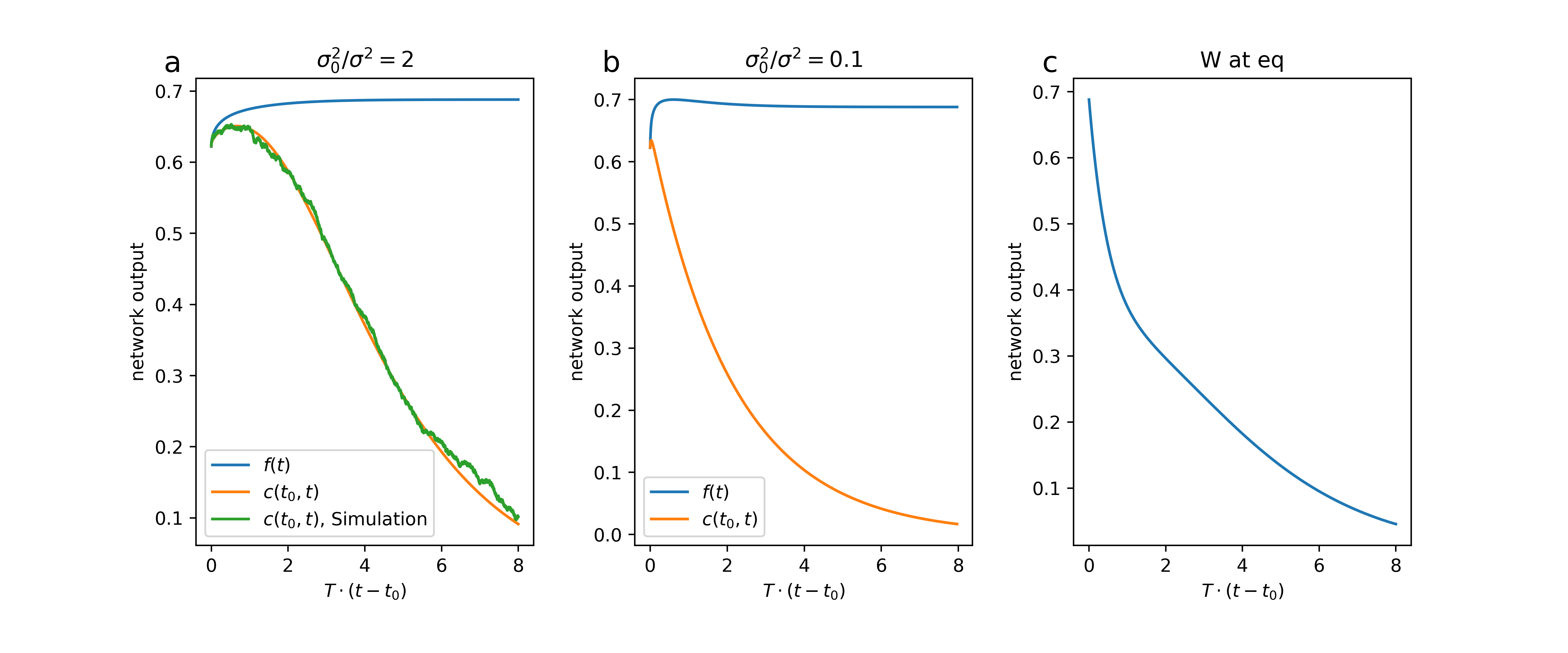
Figure 1: Temporal correlation dynamics for the synthetic dataset. (a-b) Temporal correlations between ${\bf a}_{t_{0}}$ fixed at NTK equilibrium with changing $\mathcal{W}_{t}$, for different $\sigma_{0}^{2}/\sigma^{2}$ values. In (a), we show remarkable agreement between the theory and network simulations. Interestingly, for larger $\sigma_{0}^{2}/\sigma^{2}$, the temporal correlations closely follow the mean predictor dynamics, meaning the learning of $\mathcal{W}_{t}$ is dominant in this regime. (b) There is almost exponential decay of the temporal correlations, similar to Fig.7, meaning the effect of learning on $\mathcal{W}_{t}$ is weak (almost like the representational drift case). (c) $\mathcal{W}_{t}$ fixed at NNGP equilibrium, while ${\bf a}_{t_{0}}$ changing.

Appendix C The Neural Dynamical Kernel

We focus on the large $\lambda$ limit derived above, and present several examples where the NDK has explicit expressions, and provide proofs of properties of the NDK presented in the main text.

C.1 Linear activation:

For linear activation:

$$K^{L}\left(t,t^{\prime},{\bf x},{\bf x}^{\prime}\right)=\left(m\left(t,t^{\prime}\right)\right)^{L}K^{in}\left({\bf x},{\bf x}^{\prime}\right)$$ (59)

$$\dot{K}^{L}\left(t,t^{\prime},{\bf x},{\bf x}^{\prime}\right)=I$$ (60)

The recursion relation for the NDK can be solved explicitly, yielding

$$K^{d,L}\left(t,t^{\prime},{\bf x},{\bf x}^{\prime}\right)=\left(m\left(t,t^{\prime}\right)\right)^{L}\left(L+1\right)e^{-T\sigma^{-2}\left|t-t^{\prime}\right|}K^{in}\left({\bf x},{\bf x}^{\prime}\right)$$ (61)

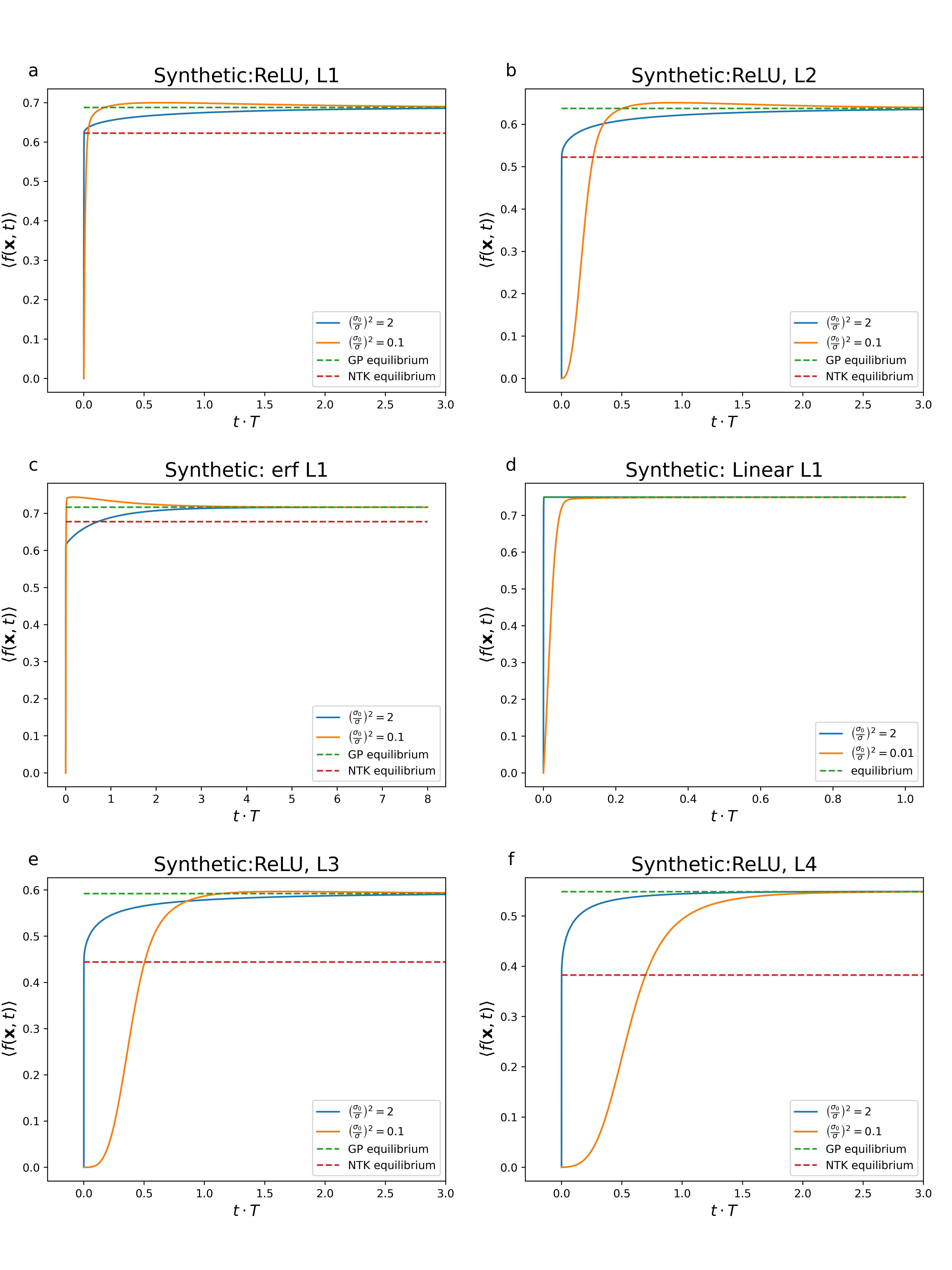
Figure 6: Examples of dynamics for different nonlinearities and depth in the synthetic dataset. (a,b,e,f) ReLU activation function for $L=1,2,3,4$, with different $\left(\sigma_{0}/\sigma\right)^{2}$ values. (c) erf activation function with different $\left(\sigma_{0}/\sigma\right)^{2}$ values. (d) Linear activation function, with different $\left(\sigma_{0}/\sigma\right)^{2}$ values. We see that with linear activation the system reaches equilibrium in a time shorter than 1/T, during the gradient-driven phase.

The NDK of linear activation is proportional to the input kernel $K^{in}\left({\bf x},{\bf x}^{\prime}\right)$ regardless of the data. The effect of network depth only changes the magnitude but not the shape of the NDK. As a result, the NNGP and NTK kernels also only differ by their magnitude, and thus the mean predictor at the NNGP and NTK equilibria only differ by $\mathcal{O}\left(T\right)$. This suggests that the diffusive phase has very little effect on the mean predictor in the low $T$ regime, as shown in Fig.6.

C.2 ReLU activation:

For ReLU activation, we define the function $J\left(\theta\right)$ [15]:

$$J\left(\theta^{L}\left(t,t^{\prime},{\bf x},{\bf x}^{\prime}\right)\right)=\left(\pi-\theta^{L}\left(t,t^{\prime},{\bf x},{\bf x}^{\prime}\right)\right)\cos\left(\theta^{L}\left(t,t^{\prime},{\bf x},{\bf x}^{\prime}\right)\right)+\sin\left(\theta^{L}\left(t,t^{\prime},{\bf x},{\bf x}^{\prime}\right)\right)$$ (62)

where the angle between ${\bf x}$ and ${\bf x}^{\prime}$ is given by :

$$\theta^{L}\left(t,t^{\prime},{\bf x},{\bf x}^{\prime}\right)=\cos^{-1}\left(\frac{m\left(t,t^{\prime}\right)}{\sqrt{m\left(t,t\right)m\left(t^{\prime},t^{\prime}\right)}}\frac{1}{\pi}J\left(\theta^{L-1}\left(t,t^{\prime},{\bf x},{\bf x}^{\prime}\right)\right)\right)$$ (63)

$\theta^{L}\left(t,t^{\prime},{\bf x},{\bf x}^{\prime}\right)$ is defined through a recursion equation, and

$$\theta^{L=0}\left(t,t^{\prime},{\bf x},{\bf x}^{\prime}\right)=\cos^{-1}\left(\frac{m\left(t,t^{\prime}\right)}{\sqrt{m\left(t,t\right)m\left(t^{\prime},t^{\prime}\right)}}\frac{K^{in}\left({\bf x},{\bf x}^{\prime}\right)}{\sqrt{K^{in}({\bf x},{\bf x})K^{in}({\bf x}^{\prime},{\bf x}^{\prime})}}\right)$$ (64)

the kernel functions are then given by

$$\dot{K}^{L}\left(t,t^{\prime},{\bf x},{\bf x}^{\prime}\right)=\frac{1}{2\pi}\left(\pi-\theta^{L}\left(t,t^{\prime},{\bf x},{\bf x}^{\prime}\right)\right)$$ (65)

$$K^{L}\left(t,t^{\prime},{\bf x},{\bf x}^{\prime}\right)=\frac{\sqrt{K^{in}\left({\bf x},{\bf x}\right)K^{in}\left({\bf x}^{\prime},{\bf x}^{\prime}\right)}}{\pi 2^{L}}\left(m\left(t,t\right)m\left(t^{\prime},t^{\prime}\right)\right)^{L/2}J\left(\theta^{L-1}\left(t,t^{\prime},{\bf x},{\bf x}^{\prime}\right)\right)$$ (66)

We obtain an explicit expression for the NDK by plugging these kernels into Eqs.$\text{\ref{eq:kd},\ref{eq:initialcond1}}.$

C.3 Error function activation

For error function activation [10]:

$$K^{L}\left(t,t^{\prime},{\bf x},{\bf x}^{\prime}\right)=\frac{2}{\pi}\sin^{-1}\left(\frac{2m\left(t,t^{\prime}\right)K^{L-1}\left(t,t^{\prime},{\bf x},{\bf x}^{\prime}\right)}{\sqrt{\left(1+2m\left(t,t\right)K^{L-1}\left(t,t,{\bf x},{\bf x}\right)\right)\left(1+2m\left(t^{\prime},t^{\prime}\right)K^{L-1}\left(t^{\prime},t^{\prime},{\bf x}^{\prime},{\bf x}^{\prime}\right)\right)}}\right)$$ (67)

$$\dot{K}_{\mu\nu}^{L}\left(t,t^{\prime},{\bf x},{\bf x}^{\prime}\right)= \frac{4}{\pi}\left(\left(1+2m\left(t,t\right)K^{L-1}\left(t,t,{\bf x},{\bf x}\right)\right)\left(1+2m\left(t^{\prime},t^{\prime}\right)K^{L-1}\left(t^{\prime},t^{\prime},{\bf x}^{\prime},{\bf x}^{\prime}\right)\right)\right.$$

$$\left.-4\left(m\left(t,t^{\prime}\right)K^{L-1}\left(t,t^{\prime},{\bf x},{\bf x}^{\prime}\right)\right)^{2}\right)^{-1/2}$$ (68)

Again we can obtain an explicit expression for the NDK by plugging these kernels into Eqs.$\text{\ref{eq:kd},\ref{eq:initialcond1}}.$

C.4 Long time behavior of the NDK

We define the long time limit as $t,t^{\prime}\rightarrow\infty,t-t^{\prime}\sim\mathcal{O}\left(T^{-1}\right)$. At a long time the statistics of $\mathcal{W}$ w.r.t. the prior becomes only a function of the time difference:

$$\left\langle\mathcal{W}_{t}\mathcal{W}_{t^{\prime}}^{\top}\right\rangle=\sigma^{2}e^{-T\sigma^{-2}\left|t-t^{\prime}\right|}=m\left(\left|t-t^{\prime}\right|\right)$$ (69)

And thus, the kernels defined above also will be only functions of the time difference. We look at the time derivative of the kernel (w.l.o.g. we assume $t>t^{\prime}$), which can be obtained with a chain rule:

$$\frac{d}{dt^{\prime}}K^{L}\left(t-t^{\prime},{\bf x},{\bf x}^{\prime}\right)=\dot{K}^{L}\left(t-t^{\prime},{\bf x},{\bf x}^{\prime}\right)\frac{d}{dt^{\prime}}\left(K^{L-1}\left(t-t^{\prime},{\bf x},{\bf x}^{\prime}\right)m\left(t-t^{\prime}\right)\right)$$ (70)

We prove by induction:

$$\frac{1}{T}\frac{d}{dt^{\prime}}\left(m\left(t-t^{\prime}\right)K^{L}\left(t-t^{\prime},{\bf x},{\bf x}^{\prime}\right)\right)=K^{d,L}\left(t-t^{\prime},{\bf x},{\bf x}^{\prime}\right)$$ (71)

The induction basis for $L=0$ is trivial. For arbitrary $L+1$:

$$\frac{1}{T}\frac{d}{dt^{\prime}}\left(m\left(t-t^{\prime}\right)K^{L+1}\left(t-t^{\prime},{\bf x},{\bf x}^{\prime}\right)\right) =m\left(t-t^{\prime}\right)\dot{K}^{L+1}\left(t-t^{\prime},{\bf x},{\bf x}^{\prime}\right)\frac{1}{T}\frac{d}{dt^{\prime}}\left(K^{L}\left(t-t^{\prime},{\bf x},{\bf x}^{\prime}\right)m\left(t-t^{\prime}\right)\right)$$

$$+e^{-T\sigma^{-2}\left(t-t^{\prime}\right)}K^{L+1}\left(t-t^{\prime},{\bf x},{\bf x}^{\prime}\right)$$ (72)

And using the induction assumption we get:

$$\frac{1}{T}\frac{d}{dt^{\prime}}\left(m\left(t-t^{\prime}\right)K^{L+1}\left(t-t^{\prime},{\bf x},{\bf x}^{\prime}\right)\right) =m\left(t-t^{\prime}\right)\dot{K}^{L+1}\left(t-t^{\prime},{\bf x},{\bf x}^{\prime}\right)K^{d,L}\left(t-t^{\prime},{\bf x},{\bf x}^{\prime}\right)$$

$$+e^{-T\sigma^{-2}\left(t-t^{\prime}\right)}K^{L+1}\left(t-t^{\prime},{\bf x},{\bf x}^{\prime}\right)$$ (73)

Which is the expression for $K^{d,L+1}\left(t-t^{\prime}\right)$. Using this identity, we can get a simple expression for the integral over $K^{d,L}\left(t-t^{\prime}\right)$ at long times:

$$\intop_{0}^{t}dt^{\prime}K^{d,L}\left(t-t^{\prime},{\bf x},{\bf x}^{\prime}\right)=\frac{\sigma^{2}}{T}K_{GP}\left({\bf x},{\bf x}^{\prime}\right)$$ (74)

C.5 NDK as a generalized two-time NTK

In Eq.11 in the main text, we claimed that the NDK has the following interpretation as a generalized two-time NTK

$$K^{d,L}\left(t,t^{\prime},{\bf x},{\bf x}^{\prime}\right)=e^{-T\sigma^{-2}\left|t-t^{\prime}\right|}\left\langle\nabla_{\Theta_{t}}f\left({\bf x},\Theta_{t}\right)\cdot\nabla_{\Theta_{t^{\prime}}}f\left({\bf x^{\prime}},\Theta_{t^{\prime}}\right)\right\rangle_{S_{0}}t\geq t^{\prime}$$ (75)

where $\langle\cdot\rangle_{S_{0}}$ denotes averaging w.r.t. the prior distribution of the parameters $\Theta$, with the statistics defined in Eq.10.

Now we provide a formal proof.

We separate $\nabla_{\Theta_{t}}f\left({\bf x},\Theta_{t}\right)$ into two parts including the derivative w.r.t. the readout weights $a_{t}$ and the hidden layer weights $\mathcal{W}_{t}$

Derivative w.r.t. the readout weights:

$$\left\langle\partial_{{\bf a}_{t}}f\left({\bf x},\Theta_{t}\right)\cdot\partial_{{\bf a}_{t^{\prime}}}f\left({\bf x},\Theta_{t^{\prime}}\right)\right\rangle_{S_{0}}=K^{L}\left(t,t^{\prime},{\bf x},{\bf x}^{\prime}\right)$$ (76)

Derivative w.r.t. the hidden layer weights:

We have

$$\partial_{{\bf W}_{t}^{l}}{\bf x}_{t}^{L}\left({\bf x},\mathcal{W}_{t}\right)=\frac{1}{\sqrt{N_{L-1}\cdots N_{l-1}}}\Pi_{k=l+1}^{L}\left[\phi^{\prime}\left(z_{t}^{k}\right){\bf W}_{t}^{k}\right]\phi^{\prime}\left(z_{t}^{l}\right){\bf x}_{t}^{l-1}$$ (77)

and

$$\left\langle\partial_{{\bf{\bf W}}_{t}^{l}}f\left({\bf x},\Theta_{t}\right)\cdot\partial_{{\bf W}_{t^{\prime}}^{l}}f\left({\bf x},\Theta_{t^{\prime}}\right)\right\rangle_{S_{0}}$$

$$=\left\langle N_{L}^{-1}{\bf a}_{t}\cdot{\bf a}_{t^{\prime}}\right\rangle\left(\Pi_{k=l+1}^{L}\left\langle N_{k}^{-1}N_{k-1}^{-1}{\bf W}_{t}^{k}\cdot{\bf W}_{t^{\prime}}^{k}\right\rangle\right)\left(\Pi_{k=l}^{L}\dot{K}^{k}\left(t,t^{\prime},{\bf x},{\bf x}^{\prime}\right)\right)K^{l-1}\left(t,t^{\prime},{\bf x},{\bf x}^{\prime}\right)$$

$$=m\left(t,t^{\prime}\right)^{L-l+1}\left(\Pi_{k=l}^{L}\dot{K}^{k}\left(t,t^{\prime},{\bf x},{\bf x}^{\prime}\right)\right)K^{l-1}\left(t,t^{\prime},{\bf x},{\bf x}^{\prime}\right)$$ (78)

To leading order in $N_{l}$ the averages over ${\bf a}$ and $\mathcal{W}$ can be performed separately for each layer, and are dominated by their prior, where each element of the weights is an independent Gaussian given by Eq.15. The term $m\left(t,t^{\prime}\right)$ comes from the covariance of the priors in $\mathcal{W}$ and ${\bf a}$, since there are a total of $L-l$ layers of $\mathcal{W}$ and one layer of ${\bf a}$, we have $m\left(t,t^{\prime}\right)^{L-l+1}$. The kernel $\dot{K}^{k}\left(t,t^{\prime},{\bf x},{\bf x}^{\prime}\right)$ comes from the inner product between $\phi^{\prime}\left(z_{t}^{k}\right)$ and $\phi^{\prime}\left(z_{t^{\prime}}^{k}\right)$, and the kernel $K^{l-1}\left(t,t^{\prime},{\bf x},{\bf x}^{\prime}\right)$ comes from the inner product between ${\bf x}_{t}^{l-1}$ and ${\bf x}_{t^{\prime}}^{l-1}$.

Using proof by induction as for the NTK [2], we obtain

$$\left\langle\partial_{\mathcal{W}_{t}}f\left({\bf x},\Theta_{t}\right)\cdot\partial_{\mathcal{W}_{t^{\prime}}}f\left({\bf x},\Theta_{t^{\prime}}\right)\right\rangle_{S_{0}}=e^{T\sigma^{-2}\left|t-t^{\prime}\right|}m\left(t,t^{\prime}\right)\dot{K}^{L}\left(t,t^{\prime},{\bf x},{\bf x}^{\prime}\right)K^{d,L-1}\left(t,t^{\prime},{\bf x},{\bf x}^{\prime}\right)$$ (79)

Combine Eq.79 with Eq.76 and with the definition of $K^{d,L}\left(t,t^{\prime},{\bf x},{\bf x}^{\prime}\right)$ in Eq.48, we have

$$e^{-T\sigma^{-2}\left|t-t^{\prime}\right|}\left\langle\nabla_{\Theta_{t}}f\left({\bf x},\Theta_{t}\right)\cdot\nabla_{\Theta_{t^{\prime}}}f\left({\bf x^{\prime}},\Theta_{t^{\prime}}\right)\right\rangle_{S_{0}}=K^{d,L}\left(t,t^{\prime},{\bf x},{\bf x}^{\prime}\right)$$ (80)

Appendix D Representational drift

To capture the phenomenon of representational drift, we consider the case where the learning signal stops at some time $t_{0}$, while the hidden layers continue to drift according to the dynamics of the prior. If all the weights of the system are allowed to drift, the performance of the mean predictor will deteriorate to chance, thus we consider stable readout weights fixed at the end time of learning $t_{0}$. This scenario can be theoretically evaluated using similar techniques to Sec.B.1 , leading to the following equation for the network output:

$$\left\langle f_{\text{drift}}\left({\bf x},t,t_{0}\right)\right\rangle=\intop_{0}^{t_{0}}\left(k^{d,L}\left({\bf x},t,t^{\prime}\right)\right)^{\top}\left(Y-\left\langle f_{\text{train}}\left(t^{\prime}\right)\right\rangle\right)$$ (81)

We see here that if $t_{0}=t$ it naturally recovers the full mean predictor. It is interesting to look at the limit where the freeze time $t_{0}$ is at NNGP equilibrium, where the network has finished its dynamics completely. In this case, the expression can be simplified due to the long time identity of the NDK (Eq.19 in the main text).

$$\left\langle f_{\text{drift}}\left({\bf x},t-t_{0}\right)\right\rangle=\left(k^{L}\left({\bf x},t-t_{0}\right)\right)^{\top}\left(IT\sigma^{-2}+K_{GP}^{L}\right)^{-1}Y$$ (82)

which has a simple meaning of two samples of hidden layer weights from different times at equilibrium. Even at long time differences, the network performance does not decrease to chance, but reaches a new static state.

$$\lim_{t-t_{0}\rightarrow\infty}\left\langle f_{\text{drift}}\left({\bf x},t-t_{0}\right)\right\rangle\rightarrow\left(k_{mean}^{L}\left({\bf x}\right)\right)^{\top}\left(IT\sigma^{-2}+K_{GP}^{L}\right)^{-1}Y$$ (83)

We can assess the network’s ability to separate classes in a binary classification task by using a linear classifier between the two distributions of outputs [71].

D.1 NTK and NNGP equilibria

The NTK and NNGP equilibria mark the initial and final points for the dynamics of the diffusive phase. An interesting question is how different these two equilibria are. In general, the answer depends on the data and the network architecture [16]. In Fig.2 we show that in these tasks deeper networks tend to favor the NNGP equilibrium compared with NTK. On the other hand, increasing the size of the training set has a similar effect on both equilibria.

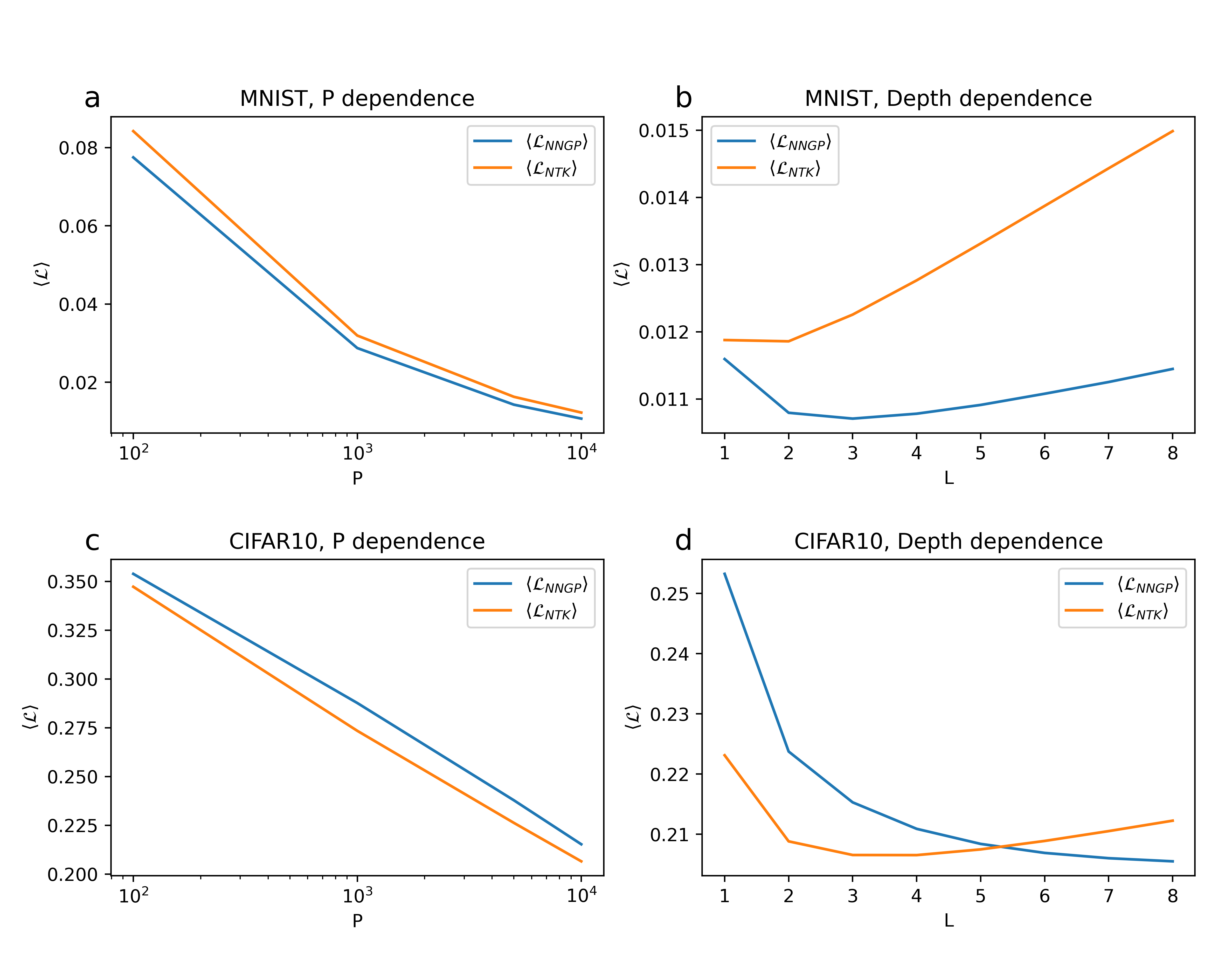
Figure 2: Comparison between NTK and NNGP equilibria, in fully connected DNNs with ReLU activation function.(a-d) The average MSE loss per test example in binary classification tasks of (a,b) MNIST dataset and (c,d) CIFAR10 dataset averaged over all class pairs. We present the results as a function of the number of training examples P (at a constant depth $L=3$) (a,c), and as a function of depth (at constant $P=10^{4}$) (b,d)

Appendix E Details of the simulations

E.1 Synthetic data

We consider $P$ normalized and orthogonal input data vectors ${\bf x}\in\mathbb{R}^{N_{0}}$, such that $K_{\mu\nu}^{in}=\frac{1}{N_{0}}{\bf x}^{\mu}\cdot{\bf x}^{\nu}=\delta_{\mu\nu}$. The labels of the data point are $\pm 1$ with equal probability. We consider a test point, which has partial overlap with one of the input vectors, and is orthogonal to all others, w.l.o.g. we assume that the test point is overlapping with the first input vector with label $+1$, such that $\frac{1}{N_{0}}{\bf x}^{test}\cdot{\bf x^{\mu}}=O_{test}\delta_{\mu,1},\frac{1}{N_{0}}{\bf x}^{test}\cdot{\bf x}^{test}=1$, and $y^{1}=+1$. In our simulations we set $O_{test}=\frac{3}{4}$, which maximizes the difference between NNGP and NTK equilibria. For this setup, we can represent the kernels by a few scalar functions:

$$K_{\mu\nu}^{d,L}\left(t,t^{\prime}\right)=k_{\text{offdiag}}^{d,L}\left(t,t^{\prime}\right)\left(1-\delta_{\mu\nu}\right)+\delta_{\mu\nu}k_{\text{diag}}^{d,L}\left(t,t^{\prime}\right)$$ (84)

$$k_{\mu}^{d,L}\left({\bf x},t,t^{\prime}\right)=k_{\text{offdiag}}^{d,L}\left(t,t^{\prime}\right)\left(1-\delta_{\mu,1}\right)+\delta_{\mu,1}k_{\text{test}}^{d,L}\left(O_{test},t,t^{\prime}\right)$$ (85)

Here $k_{{\rm offdiag}}^{d,L}(t,t^{\prime})$ and $k_{{\rm diag}}^{d,L}(t,t^{\prime})$ are off-diagonal and diagonal elements of the kernel matrix $K^{d,L}(t,t^{\prime})$, they are scalar functions of time, $k_{{\rm test}}^{d,L}(O_{test},t,t^{\prime})$ denotes the first element of the vector $k({\bf x},t,t^{\prime}),$and is also a scalar function of both time and the parameter $O_{test}$. $K_{\mu\nu}^{L}\left(t,t^{\prime}\right)$ and $\dot{K}_{\mu\nu}^{L}\left(t,t^{\prime}\right)$ have the same structure.

Because of the symmetry of this toy model, $f_{\text{train}}\left(t\right)$ takes the same value across all training points with the same label and takes the negative value for training points with the opposite label, and thus can be reduced to a scalar. We consider $f_{\text{train}}\left(t\right)$ on training points with label $+1$. We can transform the vector integral equation into a scalar one, depending only on known scalar functions:

$$f_{\text{train}}\left(t\right)=\intop_{0}^{t}dt^{\prime}\left[\left(k_{\text{diag}}^{d,L}\left(t,t^{\prime}\right)-k_{\text{diag}}^{d,L}\left(t,t^{\prime}\right)\right)\left(1-f_{train}\left(t^{\prime}\right)\right)\right]$$ (86)

$$\left\langle f\left({\bf x},\Theta_{t}\right)\right\rangle=\intop_{0}^{t}dt^{\prime}\left(k_{\text{test}}^{d,L}\left(O_{test},t,t^{\prime}\right)-k_{\text{offdiag}}^{d,L}\left(t,t^{\prime}\right)\right)\left(1-f_{train}\left(t^{\prime}\right)\right)$$ (87)

In this model the theoretical results do not depend on $P$,$N_{0}.$ For Fig.1, we vary $T$ and $\sigma,\sigma_{0}$ according to the legend, while keeping $dt=0.1$.For all other simulations presented, we use $T=0.001,$$dt=0.1$, with total time $t=10000=10/T$, $\sigma=1$, while $\sigma_{0}$ varies depending on $\left(\frac{\sigma_{0}}{\sigma}\right)^{2}$ that is presented in the plot.

E.2 MNIST

We consider a digit binary classification task [47], where one type of input is with label $+1$ and the other $-1$. In our simulations we take digits 1 and 0 as the two classes We take 50 examples from each class, flatten the image into a vector and normalize the data. The test was a held off example from the class $+1$ to make the comparison with other data sets easy (same with the synthetic data and CIFAR10).The examples in the figures are chosen for a large difference between NTK and NNGP equilibria while the error is relatively small. In Fig.2(e-g) example 25910 from MNIST data set is presented, while in Fig.4 examples 50396 (example 2) and 30508 (example 3) are presented. We used $T=0.01,$$dt=0.01$, with total time $t=1000=10/T$. In the simulations presented $\sigma=1$, while $\sigma_{0}$ varies depending on $\left(\frac{\sigma_{0}}{\sigma}\right)^{2}$ that is presented in the plot.

E.3 CIFAR10

We consider an image binary classification task [48], where one class of input is with label $+1$ and the other $-1$. In our simulations we take images of cats and dogs as the two classes. We take 50 examples from each class, flatten the image (including channels) into a vector and normalize the data. The test was a held off example from the class $+1$. The examples in the figures are chosen for a large difference between NTK and NNGP equilibria while the error compared to the true label is relatively small. In Fig.2(h) and in Fig.5 example 4484 from CIFAR10 data set is presented (example 1), while in Fig.5 examples 3287 (example 2), 5430 (example 3) and 6433 (example 4) are presented. We used $T=0.01,$$dt=0.01$, with total time $t=1000=10/T$, and $\sigma=1$, $\sigma_{0}$ varies depending on $\left(\frac{\sigma_{0}}{\sigma}\right)^{2}$ that is presented in the plot.

E.4 Langevin Dynamics

To check the validity of the theory we performed simulations with Langevin dynamics in a network with $L=1$, the network is trained under the dynamics given by Eq.8 with $lr=dt=0.01$, $T=0.001$, with total time $t=10000=10/T$ on the synthetic data introduced in SI E.1. Simulations shown in Figs.2(a) and Fig.3 are done with $P=2,N_{0}=100$, and hidden layer width $N=1000$, $\sigma_{0}^{2}/\sigma^{2}=1,2$ as indicated in the figure captions. Results are averaged over 5000 different initializations and realizations of noise. In the representational drift predictor simulations, at time $t_{0}$ the loss changes to contain only the prior part, as presented in Eq.15. The network output was calculated with the hidden layer weights at time $t$ with the readout weights at time $t_{0}$.

Appendix F Additional numerical results

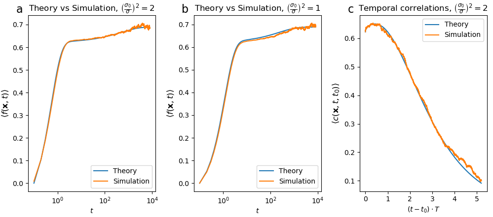
Figure 3: Theory and network simulations of the synthetic data set.(a-b) Theory and simulation of the mean predictor, for different values of $\left(\sigma_{0}/\sigma\right)^{2}$, with time in log scale due to the large difference in time scales of the two learning phases. (c) Theory and simulation of the temporal correlations of ${\bf a}_{t_{0}}$ at NTK equilibrium with $\mathcal{W}_{t}$.

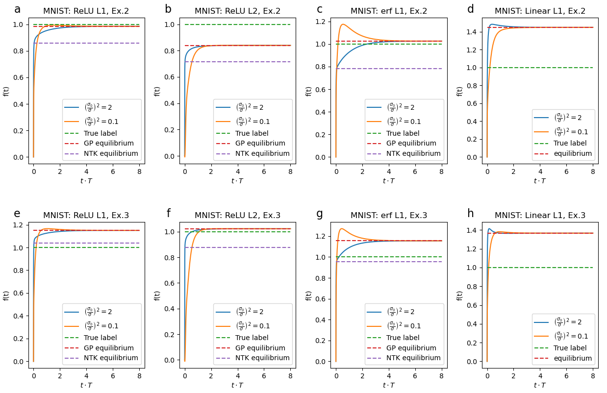
Figure 4: More test examples from MNIST dataset, for ReLU ($L=1,L=2$), erf and linear activation functions, with different $\left(\sigma_{0}/\sigma\right)^{2}$ values (a-d) Example 2, with NNGP performance better than NTK. (e-h) Example 3. Interestingly, NTK performance is better than NNGP for ReLU and erf $L=1$, but is worse for ReLU $L=2$.

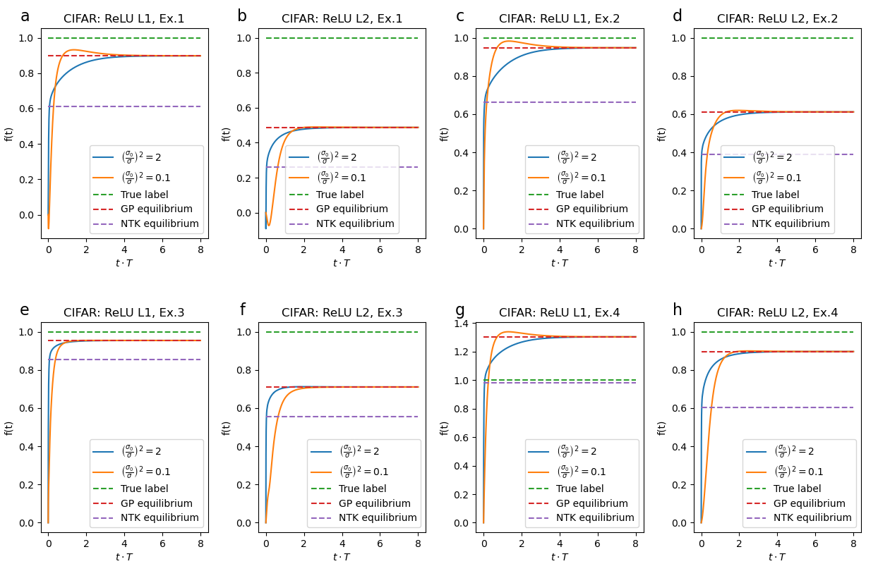
Figure 5: More test examples from CIFAR10 dataset, for ReLU activation function ($L=1,L=2$), with different $\left(\sigma_{0}/\sigma\right)^{2}$ values (a-f) Examples 1,2,3, with NNGP performance better than NTK . (g-h) Example 4. Interestingly, NTK performance is better than NNGP for ReLU $L=1$, but is worse for ReLU $L=2$.

Figure 7: The dynamics of the predictor with no external learning signal and readouts weights frozen at NTK equilibrium ($t_{0}$), for the synthetic dataset. We see an approximately exponential decay to chance level performance with time scale of $t\sim 1/T$.

References

- [1] Tamir Hazan and Tommi Jaakkola “Steps toward deep kernel methods from infinite neural networks” In arXiv preprint arXiv:1508.05133, 2015
- [2] Arthur Jacot, Franck Gabriel and Clément Hongler “Neural tangent kernel: Convergence and generalization in neural networks” In Advances in neural information processing systems 31, 2018
- [3] Jaehoon Lee et al. “Deep neural networks as gaussian processes” In arXiv preprint arXiv:1711.00165, 2017
- [4] Jaehoon Lee et al. “Wide neural networks of any depth evolve as linear models under gradient descent” In Advances in neural information processing systems 32, 2019
- [5] Alexander G de G Matthews et al. “Gaussian process behaviour in wide deep neural networks” In arXiv preprint arXiv:1804.11271, 2018
- [6] Radford M Neal “Priors for infinite networks (tech. rep. no. crg-tr-94-1)” In University of Toronto 415, 1994
- [7] Roman Novak et al. “Bayesian deep convolutional networks with many channels are gaussian processes” In arXiv preprint arXiv:1810.05148, 2018
- [8] Roman Novak et al. “Neural tangents: Fast and easy infinite neural networks in python” In arXiv preprint arXiv:1912.02803, 2019
- [9] Jascha Sohl-Dickstein, Roman Novak, Samuel S Schoenholz and Jaehoon Lee “On the infinite width limit of neural networks with a standard parameterization” In arXiv preprint arXiv:2001.07301, 2020
- [10] Christopher Williams “Computing with infinite networks” In Advances in neural information processing systems 9, 1996
- [11] Greg Yang “Wide feedforward or recurrent neural networks of any architecture are gaussian processes” In Advances in Neural Information Processing Systems 32, 2019
- [12] Lenaic Chizat and Francis Bach “Implicit bias of gradient descent for wide two-layer neural networks trained with the logistic loss” In Conference on Learning Theory, 2020, pp. 1305–1338 PMLR
- [13] Hui Jin and Guido Montúfar “Implicit bias of gradient descent for mean squared error regression with wide neural networks” In arXiv preprint arXiv:2006.07356, 2020
- [14] Hancheng Min, Salma Tarmoun, René Vidal and Enrique Mallada “On the explicit role of initialization on the convergence and implicit bias of overparametrized linear networks” In International Conference on Machine Learning, 2021, pp. 7760–7768 PMLR
- [15] Youngmin Cho and Lawrence Saul “Kernel methods for deep learning” In Advances in neural information processing systems 22, 2009
- [16] Jaehoon Lee et al. “Finite versus infinite neural networks: an empirical study” In Advances in Neural Information Processing Systems 33, 2020, pp. 15156–15172
- [17] Ziwei Ji, Justin Li and Matus Telgarsky “Early-stopped neural networks are consistent” In Advances in Neural Information Processing Systems 34, 2021, pp. 1805–1817
- [18] Mingchen Li, Mahdi Soltanolkotabi and Samet Oymak “Gradient descent with early stopping is provably robust to label noise for overparameterized neural networks” In International conference on artificial intelligence and statistics, 2020, pp. 4313–4324 PMLR
- [19] Lutz Prechelt “Early stopping-but when?” In Neural Networks: Tricks of the trade Springer, 2002, pp. 55–69
- [20] Madhu S Advani, Andrew M Saxe and Haim Sompolinsky “High-dimensional dynamics of generalization error in neural networks” In Neural Networks 132 Elsevier, 2020, pp. 428–446
- [21] Rich Caruana, Steve Lawrence and C Giles “Overfitting in neural nets: Backpropagation, conjugate gradient, and early stopping” In Advances in neural information processing systems 13, 2000
- [22] Daniel Deitch, Alon Rubin and Yaniv Ziv “Representational drift in the mouse visual cortex” In Current biology 31.19 Elsevier, 2021, pp. 4327–4339
- [23] Tyler D Marks and Michael J Goard “Stimulus-dependent representational drift in primary visual cortex” In Nature communications 12.1 Nature Publishing Group UK London, 2021, pp. 5169
- [24] Uri Rokni, Andrew G Richardson, Emilio Bizzi and H Sebastian Seung “Motor learning with unstable neural representations” In Neuron 54.4 Elsevier, 2007, pp. 653–666
- [25] Carl E Schoonover, Sarah N Ohashi, Richard Axel and Andrew JP Fink “Representational drift in primary olfactory cortex” In Nature 594.7864 Nature Publishing Group UK London, 2021, pp. 541–546
- [26] Michael E Rule, Timothy O’Leary and Christopher D Harvey “Causes and consequences of representational drift” In Current opinion in neurobiology 58 Elsevier, 2019, pp. 141–147
- [27] Shanshan Qin et al. “Coordinated drift of receptive fields in Hebbian/anti-Hebbian network models during noisy representation learning” In Nature Neuroscience Nature Publishing Group, 2023, pp. 1–11
- [28] Paul Masset, Shanshan Qin and Jacob A Zavatone-Veth “Drifting neuronal representations: Bug or feature?” In Biological Cybernetics 116.3 Springer, 2022, pp. 253–266
- [29] William Coffey and Yu P Kalmykov “The Langevin equation: with applications to stochastic problems in physics, chemistry and electrical engineering” World Scientific, 2012
- [30] Max Welling and Yee W Teh “Bayesian learning via stochastic gradient Langevin dynamics” In Proceedings of the 28th international conference on machine learning (ICML-11), 2011, pp. 681–688
- [31] Ravid Shwartz-Ziv and Naftali Tishby “Opening the black box of deep neural networks via information” In arXiv preprint arXiv:1703.00810, 2017
- [32] Marc Mézard, Giorgio Parisi and Miguel Angel Virasoro “Spin glass theory and beyond: An Introduction to the Replica Method and Its Applications” World Scientific Publishing Company, 1987
- [33] Silvio Franz, Giorgio Parisi and Miguel Angel Virasoro “The replica method on and off equilibrium” In Journal de Physique I 2.10 EDP Sciences, 1992, pp. 1869–1880
- [34] Yasaman Bahri et al. “Statistical mechanics of deep learning” In Annual Review of Condensed Matter Physics 11 Annual Reviews, 2020, pp. 501–528
- [35] Elizabeth Gardner “The space of interactions in neural network models” In Journal of physics A: Mathematical and general 21.1 IOP Publishing, 1988, pp. 257
- [36] Giuseppe Carleo et al. “Machine learning and the physical sciences” In Reviews of Modern Physics 91.4 APS, 2019, pp. 045002
- [37] Marylou Gabrié et al. “Entropy and mutual information in models of deep neural networks” In Advances in Neural Information Processing Systems 31, 2018
- [38] Luca Saglietti and Lenka Zdeborová “Solvable model for inheriting the regularization through knowledge distillation” In Mathematical and Scientific Machine Learning, 2022, pp. 809–846 PMLR
- [39] Neal Parikh and Stephen Boyd “Proximal algorithms” In Foundations and trends® in Optimization 1.3 Now Publishers, Inc., 2014, pp. 127–239
- [40] Nicholas G Polson, James G Scott and Brandon T Willard “Proximal algorithms in statistics and machine learning”, 2015
- [41] Dmitriy Drusvyatskiy and Adrian S Lewis “Error bounds, quadratic growth, and linear convergence of proximal methods” In Mathematics of Operations Research 43.3 INFORMS, 2018, pp. 919–948
- [42] Marc Teboulle “Convergence of proximal-like algorithms” In SIAM Journal on Optimization 7.4 SIAM, 1997, pp. 1069–1083
- [43] Juhan Bae, Paul Vicol, Jeff Z HaoChen and Roger B Grosse “Amortized proximal optimization” In Advances in Neural Information Processing Systems 35, 2022, pp. 8982–8997
- [44] Shun-Ichi Amari “Natural gradient works efficiently in learning” In Neural computation 10.2 MIT Press, 1998, pp. 251–276
- [45] Amir Beck and Marc Teboulle “Mirror descent and nonlinear projected subgradient methods for convex optimization” In Operations Research Letters 31.3 Elsevier, 2003, pp. 167–175
- [46] Herbert Robbins and Sutton Monro “A stochastic approximation method” In The annals of mathematical statistics JSTOR, 1951, pp. 400–407
- [47] Li Deng “The mnist database of handwritten digit images for machine learning research” In IEEE Signal Processing Magazine 29.6 IEEE, 2012, pp. 141–142
- [48] Alex Krizhevsky, Vinod Nair and Geoffrey Hinton “The CIFAR-10 dataset” In online: http://www. cs. toronto. edu/kriz/cifar. html 55.5, 2014
- [49] Michael E Rule et al. “Stable task information from an unstable neural population” In Elife 9 eLife Sciences Publications, Ltd, 2020, pp. e51121
- [50] Michael E Rule and Timothy O’Leary “Self-healing codes: How stable neural populations can track continually reconfiguring neural representations” In Proceedings of the National Academy of Sciences 119.7 National Acad Sciences, 2022, pp. e2106692119
- [51] Jingfeng Wu et al. “On the noisy gradient descent that generalizes as sgd” In International Conference on Machine Learning, 2020, pp. 10367–10376 PMLR
- [52] Hyeonwoo Noh, Tackgeun You, Jonghwan Mun and Bohyung Han “Regularizing deep neural networks by noise: Its interpretation and optimization” In Advances in Neural Information Processing Systems 30, 2017
- [53] Francesca Mignacco and Pierfrancesco Urbani “The effective noise of stochastic gradient descent” In Journal of Statistical Mechanics: Theory and Experiment 2022.8 IOP Publishing, 2022, pp. 083405
- [54] Arnak Dalalyan “Further and stronger analogy between sampling and optimization: Langevin Monte Carlo and gradient descent” In Conference on Learning Theory, 2017, pp. 678–689 PMLR
- [55] Alon Rubin et al. “Revealing neural correlates of behavior without behavioral measurements” In Nature communications 10.1 Nature Publishing Group UK London, 2019, pp. 4745
- [56] Shaul Druckmann and Dmitri B Chklovskii “Neuronal circuits underlying persistent representations despite time varying activity” In Current Biology 22.22 Elsevier, 2012, pp. 2095–2103
- [57] Matthew T Kaufman, Mark M Churchland, Stephen I Ryu and Krishna V Shenoy “Cortical activity in the null space: permitting preparation without movement” In Nature neuroscience 17.3 Nature Publishing Group US New York, 2014, pp. 440–448
- [58] Silvio Franz and Giorgio Parisi “Effective potential in glassy systems: theory and simulations” In Physica A: Statistical Mechanics and its Applications 261.3-4 Elsevier, 1998, pp. 317–339
- [59] Luca Saglietti, Stefano Sarao Mannelli and Andrew Saxe “An analytical theory of curriculum learning in teacher–student networks” In Journal of Statistical Mechanics: Theory and Experiment 2022.11 IOP Publishing, 2022, pp. 114014
- [60] Blake Bordelon and Cengiz Pehlevan “Self-consistent dynamical field theory of kernel evolution in wide neural networks” In arXiv preprint arXiv:2205.09653, 2022
- [61] Francesca Mignacco, Florent Krzakala, Pierfrancesco Urbani and Lenka Zdeborová “Dynamical mean-field theory for stochastic gradient descent in Gaussian mixture classification” In Advances in Neural Information Processing Systems 33, 2020, pp. 9540–9550
- [62] Hedy Attouch and Jérôme Bolte “On the convergence of the proximal algorithm for nonsmooth functions involving analytic features” In Mathematical Programming 116 Springer, 2009, pp. 5–16
- [63] Haozhe Shan and Blake Bordelon “A Theory of Neural Tangent Kernel Alignment and Its Influence on Training” In arXiv preprint arXiv:2105.14301, 2021
- [64] Nikhil Vyas, Yamini Bansal and Preetum Nakkiran “Limitations of the ntk for understanding generalization in deep learning” In arXiv preprint arXiv:2206.10012, 2022
- [65] Abdulkadir Canatar and Cengiz Pehlevan “A Kernel Analysis of Feature Learning in Deep Neural Networks” In 2022 58th Annual Allerton Conference on Communication, Control, and Computing (Allerton), 2022, pp. 1–8 IEEE
- [66] Qianyi Li and Haim Sompolinsky “Globally Gated Deep Linear Networks” In arXiv preprint arXiv:2210.17449, 2022
- [67] Qianyi Li and Haim Sompolinsky “Statistical mechanics of deep linear neural networks: The backpropagating kernel renormalization” In Physical Review X 11.3 APS, 2021, pp. 031059
- [68] Blake Woodworth et al. “Kernel and rich regimes in overparametrized models” In Conference on Learning Theory, 2020, pp. 3635–3673 PMLR
- [69] Shahar Azulay et al. “On the implicit bias of initialization shape: Beyond infinitesimal mirror descent” In International Conference on Machine Learning, 2021, pp. 468–477 PMLR
- [70] Timo Flesch et al. “Orthogonal representations for robust context-dependent task performance in brains and neural networks” In Neuron 110.7 Elsevier, 2022, pp. 1258–1270
- [71] Richard O. Duda, Peter E. Hart and David G. Stork “Pattern Classification” New York, NY: Wiley-Interscience, 2000