Domain walls and distances in discrete landscapes

Abstract

We explore a notion of distance between vacua of a discrete landscape that takes into account scalar potentials and fluxes via transitions mediated by domain walls. Such settings commonly arise in supergravity and string compactifications with stabilized moduli. We derive general bounds and simple estimates in supergravity which constrain deviations from the ordinary swampland distance conjecture based on moduli space geodesics, and we connect this picture to renormalization group flows via holography.

1 Introduction

Among various ideas that have emerged in the context of the swampland program [1] (see [2, 3, 4, 5, 6] for reviews), the ones related to dualities and infinite-distance limits [7, 8, 9, 10, 11, 12, 13, 14, 15, 16, 17, 18, 19] stand out for a number of reasons. To begin with, they pinpoint a specific way in which an effective field theory (EFT) breaks down due to quantum gravity effects, namely due to a tower of infinitely many species that becomes light with respect to the relevant Planck scale. Constraints for and due to this behavior can be quantified more precisely relative to more kinematical aspects of quantum gravity, such as the absence of global symmetries. Furthermore, the emergence of infinite towers at low energies can drastically modify the physics, constraining phenomenology (see e.g. [20, 21, 22, 23]) and typically leading to a new duality frame controlled by different light degrees of freedom expected to be higher-dimensional quantum fields or weakly coupled strings [24, 25, 26, 27, 28, 29]. To be more precise, the existence of light towers and the specific asymptotics of their mass scales can be considered separately, and the more quantitative statement concerns the second. A generalized version of the conjecture can be summarized by the following statement: along a divergent sequence $\{p_{n}\}$ of points in the set of vacua of some EFT consistently coupled to quantum gravity in $d$ spacetime dimensions, the mass scale of the (lighest) tower scales according to

$$\frac{m(p_{n})}{m(p_{0})}\overset{n\to\infty}{\sim}k\,e^{-\lambda\,\Delta(p_{n},p_{0})/M_{\text{pl}}^{\frac{d-2}{2}}}\,,$$ (1.1)

where $\Delta$ is a suitable distance. The positive $\mathcal{O}(1)$ constants $k\,,\,\lambda$ may be bounded in some settings [13, 15, 18], but it is important to emphasize that the peculiar exponential falloff seems to be the feature that is most closely related to string theory [30].

The aim of this paper is to explore this idea in settings where there is no exact moduli space, where $\Delta$ can be taken as the geodesic distance according to the canonical Riemannian metric. This is relevant when scalar potentials or fluxes are present, for instance in string compactifications with stabilized moduli, and establishing a generalized distance conjecture may shed light on the status of debated proposals for parametrically scale-separated stabilized vacua (see e.g. [31] on the DGKT vacuum [32], and also [33]). While this idea has been considered in various contexts [34, 35, 36, 37, 38, 39, 40, 41, 30, 31, 42], there seems to be no systematic agreed-upon way to approach the issue. Since a moduli space is a space of vacua parametrized by the expectation values of certain fields or operators, when the set of vacua is discrete our approach is to take it seriously and attempt to define a suitable notion of distance between the vacua, taking into account any ingredient that lifts the moduli space into such a discrete landscape. In order to do this, we base our construction on domain walls. If the EFT at stake contains light scalar fields $\{\phi^{i}\}$ whose moduli space with metric $G$ is lifted to a discrete set of vacua $\{\phi^{i}_{0}(\mathbf{n})\}_{\mathbf{n}\in\Gamma}$ indexed by a lattice $\Gamma$, domain walls are finite-energy solutions that interpolate between two isolated vacua. The important point is that the trajectory in field space induced by the domain wall takes into account scalar potentials and/or fluxes, so that the length of this (non-geodesic) trajectory (as defined by the metric $G$) may be interpreted as a discrete distance between two vacua in a discrete landscape. This notion has a natural holographic counterpart in the form of renormalization group (RG) flows, whose length can be computed using the (quantum) information metric [43, 39, 40, 41, 30]. Before outlining the remainder of this paper, let us emphasize that the existence of domain walls (or vacuum bubbles) is expected to be generic on the grounds of cobordism triviality [44], which means that this theoretical basis for discrete distances can extend beyond the controlled settings of Bogomol’nyi-Prasad-Sommerfield (BPS) domain walls in supergravity and holography.

With this construction at hand, we are naturally led to a discrete version of the distance conjecture. Starting with a theory that satisfies the ordinary incarnation on its moduli space, after lifting it to a discrete set of isolated vacua one can ask whether the towers of species still become light exponentially fast in the discrete distance induced by domain wall transitions. Intriguingly, this criterion can be verified entirely within the landscape of the EFT, without reference to any tower of species or ultraviolet (UV) completion. We shall see how this proposal is realized in string compactifications and how it may fail in other cases.

The contents of this paper are organized as follows. In section 2 we present the precise proposal on how to define distances between isolated vacua in a discrete landscape. In section 3 we derive some bounds and some more qualitative estimates that constrain the behavior of light towers with respect to the discrete distance for BPS domain walls in supergravity. In section 4 we discuss some simple examples, before moving to the holographic counterpart of this construction in section 5. We conclude in section 6 with some final remarks.

2 Distances in discrete vacua from domain walls

For the majority of this paper, the general setting we consider is an EFT with some light scalar fields $\{\phi^{i}\}$ described by the kinetic term

$$\mathcal{L}_{\text{kin}}=-\,\frac{1}{2}\,G_{ij}(\phi)\,\partial\phi^{i}\cdot\partial\phi^{j}\,.$$ (2.1)

The Riemannian metric $G$ is defined on the space of field values, but we consider cases in which the latter is not a moduli space. Rather, the set of vacua is discrete, lifted by a scalar potential and/or fluxes which we do not need specify yet. We assume that the set of field values takes the form $\{\phi^{i}_{0}(\mathbf{n})\}_{\mathbf{n}\in\Gamma}$, a set indexed by a lattice $\Gamma$. We denote the corresponding vacua by $|\mathbf{n}\rangle$, even though most of our discussion until section 5 is going to be (semi)classical.

In specific examples, most notably in the controlled context of minimal supergravity in four dimensions [45, 46, 47, 48, 49, 50, 51, 52], domain walls can be found as codimension-one solitons interpolating between two vacua

$$\phi^{i}_{0}(\mathbf{n}_{1})\quad\overset{\text{DW}_{\mathbf{n}_{1}\to\mathbf{n}_{2}}}{\longrightarrow}\quad\phi^{i}_{0}(\mathbf{n}_{2})$$ (2.2)

along a transverse coordinate $r$, defining a profile $\phi_{\text{DW}}(r)$ for the scalars (we suppress the index whenever possible). Singling this coordinate out, the spacetime line element induced by the backreaction of the domain wall, written in terms of $r$ and longitudinal coordinates $x$, takes the form

$$ds^{2}_{\text{DW}}=dr^{2}+e^{2A(r)}\,dx^{2}\,,$$ (2.3)

where $dx^{2}$ denotes the flat line element. Here we consider domain walls in the strict sense, flat and stationary. However, similar considerations can be made on vacuum bubbles [40] which typically arise in metastable non-supersymmetric settings.

At this point, one may be tempted to simply define the distance between the vacua $|\mathbf{n}_{1}\rangle$ and $|\mathbf{n}_{2}\rangle$ as

$$\Delta_{\text{ss}}(\mathbf{n}_{1},\mathbf{n}_{2})\equiv\int dr\,\sqrt{G_{ij}(\phi_{\text{DW}}(r))\,\frac{d\phi^{i}_{\text{DW}}}{dr}\,\frac{d\phi^{j}_{\text{DW}}}{dr}}\,,$$ (2.4)

where the subscript stands for “single step”, but this expression has a few drawbacks. To begin with, there may exist multiple domain walls interpolating between the same vacua. Borrowing terminology from flux compactifications for concreteness, $\mathbf{n}$ represents quantized charges or fluxes, and a domain wall may carry all of the net charge in a single transition or split it into several transitions. It would therefore seem ambiguous whether one should compute the distance with a single transition or summing smaller steps. In the case of exact moduli spaces, this ambiguity in the trajectory is fixed naturally by choosing geodesics. Therefore it seems reasonable to keep our definition in the discrete as close as possible, at least in spirit, to the continuous case. The second drawback actually points to a resolution: in top-down examples of flux compactifications, the Planck scale of the EFT changes as fluxes are varied because the (stabilized) volume of the internal space depends on $\mathbf{n}$. Since the expression in eq. 1.1 contains the Planck scale, it seems that the most reasonable course of action to address both issues, at least partially, is to define the distance summing along elementary domain walls, which modify the charges by a basis vector of the lattice $\mathbf{n}\to\mathbf{n}+\mathbf{e}$. If there are multiple such paths, one can minimize over them. As result, we arrive at the definition

$$\frac{\Delta(\mathbf{n}_{1},\mathbf{n}_{2})}{M_{\text{pl}}(\mathbf{n}_{2})^{\frac{d-2}{2}}}\equiv\min_{\sum_{j}\mathbf{e}_{j}=\mathbf{n}_{2}-\mathbf{n}_{1}}\sum_{k}\frac{\Delta_{\text{ss}}(\mathbf{n}_{1}+\sum_{l<k}\mathbf{e}_{l},\mathbf{n}_{1}+\sum_{l\leq k}\mathbf{e}_{l})}{M_{\text{pl}}(\mathbf{n}_{1}+\sum_{l\leq k}\mathbf{e}_{l})^{\frac{d-2}{2}}}\,,$$ (2.5)

which is meant to gradually “adjust” the Planck scale as the path moves in field space. The sum is over all steps in the chain of domain wall transitions, with the $k$-th step adding $\mathbf{e}_{k}$ to the preceding “flux”, as depicted in figure 1. This point of view was emphasized in [30] attempting to define a suitable distance beyond exact moduli spaces.

While in spirit eq. 2.5 is meant to adhere as closely as possible to the standard framework of geodesics distances in exact moduli spaces, at first glance computing such an expression in concrete examples seems daunting. However, with the aid of some inequalities and estimates, one can obtain rather general bounds that avoid explicit computations. This is the focus of the next section.

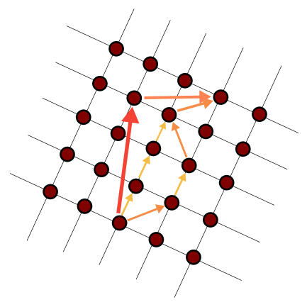
Figure 1: A sketch of multiple possible trajectories along domain wall transitions in a discrete landscape of isolated vacua. The redness of each arrow indicates the increasing charge carried by the corresponding domain wall.

3 Bounds on BPS domain walls in supergravity

As we discussed, the general expression in eq. 2.5 is quite difficult to compute in practice, and requires a numerical approach. Even if the field profiles of any domain wall solution were known in closed form, the minimization procedure would require some form of automation in general. However, we are ultimately interested in infinite-distance limits, specifically testing whether the exponential falloff of tower mass scales persists when moduli spaces are lifted to isolated vacua. Hence, it may prove useful to avoid explicit computations and provide bounds for eq. 2.5 instead. A convenient setting to attempt such task is minimal supergravity in four dimensions, where BPS domain walls are stable and characterized by simpler differential equations of the first order. In the notation of the preceding section, the BPS equations read [45, 46, 47, 48, 49, 50, 51, 52]

$$\frac{dA}{dr} =\absolutevalue{Z}\,,$$ (3.1)

$$\frac{d\phi^{i}}{dr} =-\,2\,K^{i\bar{j}}\,\partial_{\bar{j}}\absolutevalue{Z}\,,$$

where the “central charge” $Z\equiv e^{\frac{K}{2}}W$ is defined by the Kähler potential $K$ and the superpotential $W$, and attains the values $Z_{1}\,,\,Z_{2}$ at the two vacua. The cosmological constant of the resulting supersymmetric anti-de Sitter (AdS) vacua is $\Lambda=-3\absolutevalue{Z}^{2}$. Up to irrelevant proportionality factors, which we shall not consider, the “single step” distance then simplifies to

$$\Delta_{\text{ss}}(\mathbf{n}_{1},\mathbf{n}_{2})=\int dr\,\absolutevalue{\partial\absolutevalue{Z}}\,,$$ (3.2)

and involves the modulus of the gradient in field space defined by the metric $G$ induced by $K$. Here and in the following, symbols such as $\absolutevalue{\partial\absolutevalue{Z}}$ involve derivatives with respect to $\phi^{i}$. The expression in eq. 3.2 springs an intriguing observation: if the square root in the integrand were removed, the result would simply be the tension $T_{\text{DW}}$ of the domain wall, since $\absolutevalue{\partial\absolutevalue{Z}}^{2}$ is proportional to $\frac{d\absolutevalue{Z}}{dr}$ [50] (we take $\absolutevalue{Z}$ to be monotonically increasing for definiteness). On the other hand, as we will discuss in section 5, a natural holographic counterpart of the domain wall distance is the length of its dual RG flow [55, 56, 57, 58, 59]. The analog of the quantum information distance [43, 39, 41] (see also [60] for a related notion) with the square root removed was investigated in [61], where it was shown that the corresponding “length” yields the difference in $a$-central charges of the conformal field theories (CFTs) at the endpoints of the flow. This matches nicely with the known holographic dictionary, since $\absolutevalue{Z}$ in supersymmetric AdS vacua is in fact dual to the central charge [50]. While this perspective is simple, independent of the specific field profiles $\phi_{\text{DW}}(r)$ and avoids essentially all of the computational difficulties of eq. 2.5, we stick to the approach that, in our view, is closest in spirit to the established geometry of exact moduli spaces.

In order to find useful bounds from BPS domain walls, let us focus on the “single step” distance $\Delta_{\text{ss}}$ first. In the following, all arbitrary functions of $r$ are chosen to be sufficiently “nice” in the sense that all integrals converge.

3.1 Upper bounds

Let us consider the Cauchy-Schwarz inequality

$$\norm{fg}_{1}\leq\norm{f}_{2}\,\norm{g}_{2}\,,$$ (3.3)

applied to the functions

$$f=\sqrt{\varphi}\,,\qquad g=\frac{\absolutevalue{\partial\absolutevalue{Z}}}{\sqrt{\varphi}}$$ (3.4)

for some positive function of the form $\varphi(\absolutevalue{Z(r)})$. Therefore, up to the prefactor in eq. 3.2, the left-hand side of eq. 3.4 is $\Delta_{\text{ss}}$, and one obtains

$$\Delta_{\text{ss}}^{2}\leq\left(\int\varphi\,dr\right)\left(\int\absolutevalue{\partial\absolutevalue{Z}}^{2}\,\varphi^{-1}\,dr\right)\,.$$ (3.5)

This expression is useful, because the last integral can be rewritten (again up to an irrelevant prefactor) as

$$\int\absolutevalue{\partial\absolutevalue{Z}}^{2}\,\varphi(\absolutevalue{Z})^{-1}\,dr\propto\int_{\absolutevalue{Z_{1}}}^{\absolutevalue{Z_{2}}}\varphi(\absolutevalue{Z})^{-1}\,d\absolutevalue{Z}\,,$$ (3.6)

which is independent of the field profile $\phi_{\text{DW}}(r)$ induced by the domain wall. Unfortunately we did not find a simple inequality that only involves such integrals, but the other one can be estimated as we shall now argue. Firstly, $\varphi$ must be chosen so that both integrals (which involve two different integration variables) converge. Linearizing the BPS equations around the AdS vacua, one finds that the approach to the fixed points $Z_{1}\,,\,Z_{2}$ is exponential in $r$. Thus, one may pick

$$\varphi(\absolutevalue{Z})=\frac{1}{1+\log^{2}\left(\frac{\absolutevalue{Z}-\absolutevalue{Z_{1}}}{\absolutevalue{Z_{2}}-\absolutevalue{Z}}\right)}\,,$$ (3.7)

which decays as $r^{-2}$ as a function of $r$ and whose reciprocal $\varphi^{-1}$ has integrable singularities as a function of $\absolutevalue{Z}$. As a result, the last integral in eq. 3.5 gives

$$\int_{\absolutevalue{Z_{1}}}^{\absolutevalue{Z_{2}}}\varphi^{-1}(\absolutevalue{Z})\,d\absolutevalue{Z}=\left(1+\frac{\pi^{2}}{3}\right)\Delta\absolutevalue{Z}\propto T_{\text{DW}}\,.$$ (3.8)

All in all, we arrive at

$$\Delta_{\text{ss}}\leq k\,\sqrt{T_{\text{DW}}}\left(\int\frac{dr}{1+\log^{2}\left(\frac{\absolutevalue{Z}-\absolutevalue{Z_{1}}}{\absolutevalue{Z_{2}}-\absolutevalue{Z}}\right)}\right)^{\frac{1}{2}}\,,$$ (3.9)

where $k$ subsumes all numerical (and calculable) prefactors. In this derivation we have assumed that $\absolutevalue{Z}$ is regular, but in the case of flux vacua membranes can carry the missing charge along a transition and induce a discontinuity [51]. In this case $\frac{d\absolutevalue{Z}}{dr}=4\,\absolutevalue{\partial\absolutevalue{Z}}^{2}+\frac{1}{2}\,T_{\text{M}}$, where $T_{\text{M}}\leq T_{\text{DW}}$ is the membrane tension. As a result eq. 3.6 has an additional negative term proportional to $T_{\text{M}}$, which can be removed at the price of replacing the equal sign with $\leq$. Therefore, the final bound in eq. 3.9 still holds.

3.1.1 Upper bound estimates

So far, the inequalities we derived hold up to numerical constants which do not depend on any parameters. These factors may be easily reinstated in the above expressions, but they are irrelevant since we are ultimately interested in large-distance scalings. In order to massage the above expressions into more useful bounds, we now estimate the integral in eq. 3.9 using the rough behavior of $\absolutevalue{Z(r)}$. Since the approach to the fixed points is exponentially fast,

$$\absolutevalue{Z} \overset{r\,\to\,+\infty}{\sim}\absolutevalue{Z}_{+}\equiv\absolutevalue{Z_{2}}-A_{2}\,e^{-\alpha_{2}r}\,,$$ (3.10)

$$\absolutevalue{Z} \overset{r\,\to\,-\infty}{\sim}\absolutevalue{Z}_{-}\equiv\absolutevalue{Z_{1}}+A_{1}\,e^{\alpha_{1}r}\,,$$

we approximate $\absolutevalue{Z}\approx\frac{\absolutevalue{Z_{1}}+\absolutevalue{Z_{2}}}{2}$ in a central region $r_{-}<r<r_{+}$ and $\absolutevalue{Z}\approx\absolutevalue{Z_{\pm}}$ outside, where $r_{+}\equiv\max(0\,,-\frac{1}{\alpha_{2}}\log\frac{\Delta\absolutevalue{Z}}{A_{2}})$ and $r_{-}\equiv\min(0\,,\frac{1}{\alpha_{1}}\log\frac{\Delta\absolutevalue{Z}}{A_{1}})$ are chosen to make $\varphi(\absolutevalue{Z_{\pm}})$ well-defined. Hence, the approximated integral with the choice of eq. 3.7 is

$$\int\varphi(\absolutevalue{Z})\,dr =\int_{0}^{+\infty}\varphi(\absolutevalue{Z})\,dr+\int_{-\infty}^{0}\varphi(\absolutevalue{Z})\,dr$$ (3.11)

$$\approx\int_{r_{+}}^{+\infty}\varphi(\absolutevalue{Z}_{+})\,dr+\int_{r_{-}}^{r_{+}}1\,dr+\int_{-\infty}^{r_{-}}\varphi(\absolutevalue{Z}_{-})\,dr\,.$$

After a change of variables, the first and last terms simplify to ($i=1\,,\,2)$

$$\frac{1}{\alpha_{i}}\int_{0}^{\min(1\,,\,x_{i})}\frac{1}{1+\log^{2}\left(\frac{u}{x_{i}-u}\right)}\frac{du}{u}\leq\frac{\pi}{2\alpha_{i}}\,,\qquad x_{i}\equiv\frac{\Delta\absolutevalue{Z}}{A_{i}}\,.$$ (3.12)

The remainder $r_{+}-r_{-}$ can be upper-bounded by $\frac{1}{\alpha_{2}}\absolutevalue{\log\frac{\Delta\absolutevalue{Z}}{A_{2}}}+\frac{1}{\alpha_{1}}\absolutevalue{\log\frac{\Delta\absolutevalue{Z}}{A_{1}}}$. All in all, a weaker and approximate version of the upper bound of eq. 3.9 takes the simple form

$$\Delta_{\text{ss}}\lesssim\sqrt{\frac{T_{\text{DW}}}{\alpha_{1}}\left(\frac{\pi}{2}+\absolutevalue{\log\frac{\Delta\absolutevalue{Z}}{A_{1}}}\right)+\frac{T_{\text{DW}}}{\alpha_{2}}\left(\frac{\pi}{2}+\absolutevalue{\log\frac{\Delta\absolutevalue{Z}}{A_{2}}}\right)}\,.$$ (3.13)

3.1.2 Scalings at large fluxes

Let us now further assume that the stabilization arises from fluxes, as usual in compactifications arising from string theory or string-inspired models. At large flux, say along a specific direction $\mathbf{n}=n\,\mathbf{e}$ with $n\gg 1$, at AdS vacua one typically has $\absolutevalue{Z}\propto n^{-\gamma}$ for some $\gamma<0$.

In order to estimate the scaling with $n$ of the approximate upper bound of eq. 3.13, we observe that for an elementary transition $\Delta\absolutevalue{Z}\sim\frac{d\absolutevalue{Z}}{dn}\propto n^{-\gamma-1}$, while $\alpha_{1}\sim\alpha_{2}$ arise linearizing the BPS equations for $\phi^{i}_{\text{DW}}\sim\phi_{0}^{i}+\delta\phi^{i}$ around the AdS vacua, which brings along the Hessian matrix of $\absolutevalue{Z}$ from eq. 3.1. Since $\frac{d}{dr}\absolutevalue{Z}\propto\absolutevalue{\partial\absolutevalue{Z}}^{2}\propto\absolutevalue{\frac{d}{dr}\delta\phi}^{2}$, the exponents $\alpha_{i}$ are twice the maximum or minimum eigenvalues of the Hessian matrix of $\absolutevalue{Z}$, depending on whether $r\to+\infty$ or $r\to-\infty$.

If $\phi^{i}$ represent (pseudo-)moduli for volumes of internal (holomorphic) cycles in an “electric” frame, one typically expects them to scale as the Kaluza-Klein (KK) scale $\ell_{\text{KK}}^{2}$. For instance, the Kähler moduli $t^{a}$ of a Calabi-Yau compactification from ten dimensions to four dimensions satisfy $D_{abc}t^{a}t^{b}t^{c}=\text{Vol}(\text{CY}_{3})\propto\ell_{\text{KK}}^{6}$, assuming no significant deviations from isotropy. The dual “magnetic” moduli $\tau_{a}=D_{abc}t^{b}t^{c}$ scale differently. Thus, if $m_{\text{KK}}\sim n^{-\beta}$ is the curvature scale of the internal space, with $\beta>0$, a schematic estimate for the exponents $\alpha$ is $\absolutevalue{Z}/\phi_{0}^{2}\propto n^{4\beta-\gamma}$. This leads to

$$\Delta_{\text{ss}}\lesssim n^{2\beta-\frac{1}{2}}\,\sqrt{\log n}\,.$$ (3.14)

To connect to the formula of eq. 2.5, we also need the relation $M_{\text{pl}}^{d-2}(\mathbf{n})\propto\ell_{\text{KK}}^{p}$, where $p$ denotes the internal dimensions. Since this relation holds at the level of the $(d+p)$-dimensional EFT, we expect the supersymmetric case with $d=4$ to have $p\leq 6$ and even. According to eq. 2.5, one needs to multiply by $\frac{1}{n^{\frac{\beta p}{2}}}$ and sum over $n$ from $n_{1}$ to $n_{2}$. The final result is the approximate upper bound

$$\frac{\Delta(n_{1},n_{2})}{M_{\text{pl}}(n_{2})} \lesssim\sum_{n=n_{1}}^{n_{2}}n^{(2-\frac{p}{2})\beta-\frac{1}{2}}\sqrt{\log n}$$ (3.15)

$$\underset{\beta\neq\frac{1}{p-4}}{\overset{n_{2}\gg n_{1}}{\sim}}n_{2}^{(2-\frac{p}{2})\beta+\frac{1}{2}}\sqrt{\log n_{2}}\,,$$

where the asymptotics is given up to a numerical prefactor. If $\beta=\frac{1}{p-4}$, the leading asymptotics is instead given by $\log^{\frac{3}{2}}n_{2}$. For definiteness, the interesting case $p=6$ gives $n_{2}^{-\beta+\frac{1}{2}}\sqrt{\log n_{2}}$ for $\beta\neq\frac{1}{2}$.

The scaling corresponding to a discrete version of the distance conjecture is logarithmic. To wit, since all masses are expected to scale with a power of $n$, the result would be an exponential decay in $\Delta/M_{\text{pl}}$. From eq. 3.15 we see that there is a window for such scaling, insofar as the exponent of $n_{2}$ is non-negative. This means that, within the assumptions that led to this estimate, assuming the distance conjecture for ordinary moduli spaces holds, a discrete distance conjecture for BPS domain walls can only hold if

$$(p-4)\beta<1\,,$$ (3.16)

which in the most interesting case $p=6$ of ten-dimensional $\mathcal{N}=1$ compactification entails $\beta<\frac{1}{2}$. As an example, the DGKT vacuum has $\beta=\frac{1}{4}$ [32], but the string coupling $g_{s}\propto n^{-\frac{3}{4}}$ also depends on $n$. Adjusting for this, the new bound on the discrete distance is $\Delta/M_{\text{pl}}\lesssim\sqrt{\frac{\log n_{2}}{n_{2}}}$, which would seem in tension with an exponential decay or even with the existence of an infinite-distance limit. However, before drawing conclusions from this result, let us emphasize that the DGKT construction contains other ingredients that should be taken into account, such as complex structure moduli (in the case of Calabi-Yau orientifolds) blow-up moduli (in the case of $T^{6}/\mathbb{Z}_{3}^{2})$, smearing and/or additional fields, and these additional elements may modify the results. For instance, the inclusion of open-string (pseudo-)moduli in the EFT arising from D4-branes [31] leads to geodesic distances that do scale logarithmically with $n$. Indeed, these moduli do not have the same geometrical interpretation, and the above estimates cannot be applied anymore. After the field redefinition that brings the field space metric of [31] to the canonical one on $\mathbb{H}^{2}\times\mathbb{R}$, the corresponding field scales has scaling exponent $\beta=1$, which modifies the upper bound for the “single step” distance $\Delta_{\text{ss}}$ to $\Delta_{\text{ss}}/M_{\text{pl}}\lesssim\sqrt{\log n}$. Hence, the total distance $\Delta/M_{\text{pl}}\lesssim n_{2}\,\sqrt{\log n_{2}}$, which is now compatible with the results of [31].

Another, more general, consideration is that by AdS/CFT holography one expects the central charge of the dual CFT to scale as $c\propto\ell_{\text{AdS}}^{2}\propto n^{2\gamma}$. If scale separation is absent $\gamma=\beta$ and the EFT would be replaced by a consistent truncation. As a result, the bound $\beta<\frac{1}{2}$ would entail that the central charge $c\ll n$. Generally speaking, it seems difficult to realize a holographic central charge with this property. The typical behaviors of central charges can only be compatible with our analysis if $\gamma>\beta$, that is $\ell_{\text{AdS}}\gg\ell_{\text{KK}}$.

3.2 Lower bounds

Let us now discuss lower bounds on the discrete distance, starting from the “single step” quantity $\Delta_{\text{ss}}$. This time we consider the reverse Hölder inequality,

$$\norm{f\,g}_{1}\geq\norm{f}_{\frac{1}{q}}\,\norm{g}_{-\frac{1}{q-1}}\,,\qquad q>1$$ (3.17)

applied to the functions

$$f=\absolutevalue{\partial\absolutevalue{Z}}^{q+1}\,\varphi\,,\qquad g=\absolutevalue{\partial\absolutevalue{Z}}^{1-q}\,.$$ (3.18)

Writing out the integrals explicitly, one obtains

$$\int\absolutevalue{\partial\absolutevalue{Z}}^{2}\,\varphi\,dr\geq\left(\int\absolutevalue{\partial\absolutevalue{Z}}^{1+\frac{1}{q}}\,\varphi^{\frac{1}{q}}\,dr\right)^{q}\left(\int\absolutevalue{\partial\absolutevalue{Z}}\,dr\right)^{1-q}\,,$$ (3.19)

which gives the (family of) lower bound(s)

$$\Delta_{\text{ss}}\geq\left(\frac{\int\absolutevalue{\partial\absolutevalue{Z}}^{1+\frac{1}{q}}\,\varphi^{\frac{1}{q}}\,dr}{\int\absolutevalue{\partial\absolutevalue{Z}}^{2}\,\varphi\,dr}\right)^{\frac{1}{q-1}}\int\absolutevalue{\partial\absolutevalue{Z}}^{1+\frac{1}{q}}\,\varphi^{\frac{1}{q}}\,dr\,.$$ (3.20)

Taking $q\to+\infty$, a straightforward expansion gives the simpler bound

$$\Delta_{\text{ss}}\geq e^{-\frac{\int\absolutevalue{\partial\absolutevalue{Z}}^{2}\,\varphi\,\log(\absolutevalue{\partial\absolutevalue{Z}}\,\varphi)\,dr}{\int\absolutevalue{\partial\absolutevalue{Z}}^{2}\,\varphi\,dr}}\int\absolutevalue{\partial\absolutevalue{Z}}^{2}\,\varphi\,dr\,,$$ (3.21)

where once again the last factor rearranges into an integral that does not depend on the profile $\phi_{\text{DW}}(r)$ choosing $\varphi=\varphi(\absolutevalue{Z})$. The exponent can be interpreted as the average $\langle\log(\absolutevalue{\partial\absolutevalue{Z}}\,\varphi)\rangle_{\rho}$ with respect to the probability distribution with (non-normalized) density $\rho=\absolutevalue{\partial\absolutevalue{Z}}^{2}\,\varphi$, and thus letting $M\equiv\sup_{r}\absolutevalue{\partial\absolutevalue{Z}}\,\varphi$, if $M$ is finite one has

$$e^{-\langle\log(\absolutevalue{\partial\absolutevalue{Z}}\,\varphi)\rangle_{\rho}}\geq e^{-\log M}=\frac{1}{M}\,.$$ (3.22)

Therefore, up to a numerical (and calculable) prefactor $k$, one arrives at the weaker bound

$$\Delta_{\text{ss}}\geq\frac{k}{M}\int_{\absolutevalue{Z_{1}}}^{\absolutevalue{Z_{2}}}\varphi(\absolutevalue{Z})\,d\absolutevalue{Z}\,.$$ (3.23)

Once again, this bound holds assuming $\absolutevalue{Z}$ is regular. In the presence of discontinuities induced by membranes, these steps are not well-defined due to the appearance of $\delta$-distributions in rational powers or logarithms.

3.2.1 Lower bound estimates and flux scalings

In order to estimate $M$ precisely one would need to know either the width or the peak slope of the kink profile of $\absolutevalue{Z}$. One expects $\absolutevalue{\partial\absolutevalue{Z}}$ to be sharply peaked and decay exponentially, and thus choosing a slowly-varying (or outright constant) $\varphi$ would allow estimating $M$ with the height of the peak. By contrast, choosing $\varphi$ to be a window function that vanishes around the peak would avoid the need to know its height, but this requires knowing its width.

To obtain some qualitative insights from eq. 3.23, we take the first approach and estimate the height of the peak in $\absolutevalue{\partial\absolutevalue{Z}}$ as the average slope $\frac{\absolutevalue{\Delta\absolutevalue{Z}}}{\absolutevalue{\Delta\phi}}\propto\frac{T_{\text{DW}}}{\absolutevalue{\Delta\phi}}$. Choosing a constant $\varphi$ then simplifies eq. 3.23 to $\Delta_{\text{ss}}\gtrsim\absolutevalue{\Delta\phi}$.

In terms of the flux scalings discussed in section 3.1.2, $\absolutevalue{\Delta\phi}\sim\absolutevalue{\frac{d\phi}{dn}}\sim n^{2\beta-1}$. Putting together the lower bound of eq. 3.23 and the upper bound of eq. 3.14, one arrives at the approximate inequalities

$$n^{2\beta-1}\lesssim\Delta_{\text{ss}}\lesssim n^{2\beta-\frac{1}{2}}\,\sqrt{\log\,n}\,,$$ (3.24)

which can then be turned into a bound for the bulk total distance according to eq. 2.5 as in eq. 3.15. Dividing by the Planck mass changes the exponents in the lower bound as in eq. 3.15, and since $\beta>0$ the resulting expression $n^{(2-\frac{p}{2})\beta-1}$ would suggest that, in order for a discrete distance conjecture to hold, the number of extra dimensions has to be at $p\geq 4$. Otherwise, the scaling of the lower bound would exclude a logarithmic behavior $\Delta_{\text{ss}}/M_{\text{pl}}\sim n^{-1}$, or equivalently $\Delta(n_{1},n_{2})\sim\log\frac{n_{2}}{n_{1}}$. Of course the validity of these considerations is somewhat shaky, since the estimates beyond the sharp bounds derived from Hölder’s inequalities are not under control quantitatively.

4 Examples on hyperbolic field spaces

As we have seen, the bounds that we were able to derive on general grounds are not very constraining, including the simpler estimates based on large-flux scalings. It is instructive to consider more concrete examples, in which one can derive more stringent bounds.

We will focus on hyperbolic field spaces, which are ubiquitous in supersymmetric compactifications due to the properties of nilpotent orbits [64]. The fields arrange into pairs of axions and saxions $(a,s)$ with line element

$$ds^{2}_{\mathbb{H}^{2}}=\frac{da^{2}+ds^{2}}{s^{2}}\,.$$ (4.1)

The “single step” distance $\Delta_{\text{ss}}$ can be now bounded in a much simpler manner, using the inequalities $\max(\absolutevalue{x}\,,\,\absolutevalue{y})\leq\sqrt{x^{2}+y^{2}}\leq\absolutevalue{x}+\absolutevalue{y}$. Taking the field profiles to be increasing for definiteness, one obtains

$$\max\left(\int\frac{da}{s}\,,\,\log\frac{s(\mathbf{n_{2}})}{s(\mathbf{n_{1}})}\right)\leq\Delta_{\text{ss}}\leq\int\frac{da}{s}+\log\frac{s(\mathbf{n_{2}})}{s(\mathbf{n_{1}})}\,.$$ (4.2)

This bound can be weakened and simplified by taking maximum and minimum values of $s$ in the integrals, which yields

$$\max\left(\frac{\Delta a}{s(\mathbf{n_{2}})}\,,\,\log\frac{s(\mathbf{n_{2}})}{s(\mathbf{n_{1}})}\right)\leq\Delta_{\text{ss}}(\mathbf{n_{1}},\mathbf{n_{2}})\leq\frac{\Delta a}{s(\mathbf{n_{1}})}+\log\frac{s(\mathbf{n_{2}})}{s(\mathbf{n_{1}})}\,.$$ (4.3)

For ordinary trajectories dominated by saxions, at large moduli space distances $s\to+\infty$ as a power $n^{\alpha}$ while $\Delta a\ll 1$. Thus, if $\alpha\geq 1$ the logarithmic terms dominate, since

$$\log\frac{s((n+1)\,\mathbf{e})}{s(n\,\mathbf{e})}\sim\frac{\alpha}{n}\,,$$ (4.4)

and the domain wall distance scales as the geodesic distance. Instead, if $\alpha<1$ the axionic terms can dominate if $\Delta a=\mathcal{O}(1)$, and the discrete distance conjecture would not follow from the ordinary one. This is actually an known result in a new guise: this kind of non-geodesicity for hyperbolic field spaces was explored in [36] and was referred to a the swampy case.

In the spirit of applying our considerations beyond string compactifications, let us also consider the toy model studied in [51]. The model contains a single complex modulus $\phi$ with $\imaginary\phi>0$, the bosonic component of a chiral superfield, with hyperbolic Kähler potential $K=-\,\log\imaginary\phi$, and a linear flux superpotential

$$W=(e_{0}+i\,m^{1})-i\,(e_{1}+i\,m^{0})\,\phi$$ (4.5)

containing two electric integer fluxes $e_{0}\,,\,e_{1}$ and two magnetic integer fluxes $m^{0}\,,m^{1}$. The model has a discrete landscape of vacua (depicted in figure 2), which is most conveniently parametrized by the complex fluxes $\alpha_{0}\equiv e_{0}-i\,m^{1}$ and $\alpha_{1}\equiv e_{1}-i\,m^{0}$. The field stabilizes at

$$\phi_{0}=i\,\frac{\alpha_{0}}{\alpha_{1}}\,,$$ (4.6)

with the constraint $\imaginary\phi_{0}=\frac{\real\alpha_{0}\overline{\alpha_{1}}}{\absolutevalue{\alpha_{1}}^{2}}>0$. It is possible to go to infinite distance in field space via elementary domain wall transitions if the fluxes in one of the two complex combinations $\alpha$ scales with $n$, which means that, up to $SL(2,\mathbb{Z})$ inversions, the exponent $\beta=1$. This model contains no explicit reference to a flux-dependent Planck scale, and in this case the bounds of eq. 3.24 would seem to exclude a logarithmic scaling, at least insofar as the estimates behind eq. 3.24 are reliable. However, in this model the domain walls carrying the missing charge feature a discontinuity, which is induced by a membrane of tension $T_{\text{M}}\leq T_{\text{DW}}$. As a result, as discussed in section 3.2, the lower bound eq. 3.23 does not apply. To understand more intuitively what is happening, the lower-bound estimate in eq. 3.24 relies on the finiteness of $M$ in eq. 3.23, but since $\absolutevalue{Z}$ is discontinuous at the origin one can think of a “divergent $M$” trivializing the bound. Indeed, as shown in [51], there are elementary domain walls between vacua that are “vertically aligned”, in the sense of figure 2. Along such transitions only the saxions flow between flux minima according to $s_{0}(n)\to s_{0}(n)+1$, implying that $\Delta_{\text{ss}}\sim\frac{1}{n}$ up to a factor. This recovers the geodesic logarithmic scaling of the full distance $\Delta(n_{1},n_{2})\sim\log\frac{n_{2}}{n_{1}}$. This should be the universal scaling at large distances in this model, because of the considerations on axion variations discussed above.

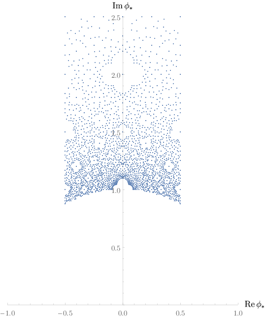
Figure 2: The discrete landscape of isolated vacua in the simple model above eq. 4.5. The plot is taken from the original reference [51].

4.1 Replacing hyperbolic space with flat space

In order to explore the relevance of hyperbolic field spaces in the above example, let us modify the model replacing it with a flat field space, with

$$ds^{2}_{\mathbb{H}^{2}}\quad\longrightarrow\quad da^{2}+ds^{2}\,.$$ (4.7)

The corresponding Kälher potential is $K=\absolutevalue{\phi}^{2}$. Thus, supersymmetric vacua obey

$$\partial W+\partial K\,W=-i\,\overline{\alpha_{1}}+\overline{\phi}\,W=0\,,$$ (4.8)

and for large fields (driven by some fluxes going to infinity) the first term is negligible. Hence, the solutions asymptote to $\phi\sim-i\,\frac{\overline{\alpha_{0}}}{\overline{\alpha_{1}}}$. To ensure that the field be self-consistently large, we take e.g. $\alpha_{1}=1$ and $\alpha_{0}=-i\,n$. We also need the first correction to compute the leading on-shell superpotential, and it reads

$$\phi\sim-i\,\frac{\overline{\alpha_{0}}}{\overline{\alpha_{1}}}+i\,\frac{\alpha_{1}}{\alpha_{0}}=n-\frac{1}{n}\,.$$ (4.9)

For this choice of fluxes, the other solution is not large for $n\gg 1$. The distance along increasing $n$ is now $\Delta\phi\sim n$, while the central charge

$$\absolutevalue{Z}=e^{K}\absolutevalue{W}\sim\frac{1}{n}\,e^{n^{2}-2}\,.$$ (4.10)

While for both flat and hyperbolic field spaces the cosmological constant grows in the large-$n$ limit, the exponential scaling with the distance is now replaced by $\exp\Delta^{2}$. This means that a modified model where the distance conjecture is satisfied would likely become inconsistent replacing the hyperbolic field space with a flat one, since it would bring along a factor $e^{\absolutevalue{\phi}^{2}}$ in the cosmological constant and dramatically change the distance scalings.

All in all, we see that EFTs with hyperbolic field spaces, at least insofar as the Planck scale does not strongly depend on $n$ (perhaps with stabilization induced by a potential), appear to be especially compatible with a discrete distance conjecture. It seems easy to violate the required scalings if the field spaces are not hyperbolic or the fields do not scale logarithmically with $n$. Typically, geometric moduli which appear in hyperbolic field spaces scale as powers of $n$ at stabilized points, while the dilaton is canonically normalized but typically stabilizes logarithmically in $n$. This phenomenon has been observed in non-supersymmetric compactifications as well [37, 40], where the discrete distance still scales logarithmically due to bounds very similar to eq. 4.3. If the discrete version of the distance conjecture will be put on a more solid footing, these hints may point to a universal structure of consistent (supersymmetric) EFTs which seems to nicely match the top-down understanding gathered in [64, 66, 67, 68, 69, 70].

5 Holographic RG flows

There is a natural holographic counterpart of the ideas that we have discussed. (BPS) domain walls between (supersymmetric) AdS vacua are typically associated with RG flows between the corresponding dual CFTs. The quantum information metric [71, 43, 72, 73, 74, 75, 41] is a natural extension of the Zamolodchikov metric [76] which allows, for example, to compute distances between theories along RG flows [40, 30]. There is also a slightly different approach in the same spirit, described in [60], where the renormalization group scale is taken into account explicitly in the metric.

A holographic test of the discrete distance conjecture involves computing this distance summing over “single step” RG flows, dividing by the $C_{T}$ central charge defined by the stress-tensor correlator in order to account for bulk Planck units [12, 30]. If the resulting distance turns out to scale as $\log\,N$, with $N\gg 1$ the number of colors in the dual gauge theory (more generally some power of the central charge related to $n$ in the bulk), the discrete distance conjecture also reproduces the “AdS distance conjecture” of [35] using a notion of distance that takes into account the isolation of vacua.

5.1 Test in $\mathcal{N}=4$ super Yang-Mills

The simplest setting to assess our proposal from a dual perspective is $U(N)$ $\mathcal{N}=4$ super Yang-Mills (SYM) and its dual bulk supergravity in AdS₅. The elementary domain walls interpolate between the vacuum with flux quanta $N$ and $N+1$. On the CFT side, this should correspond to an RG flow interpolating between $U(N)$ and $U(N+1)$. The microscopic picture consists of separating one out of $N+1$ coincident D3-branes from the remaining stack of $N$, Higgsing the gauge theory. The setup is depicted in figure 3.

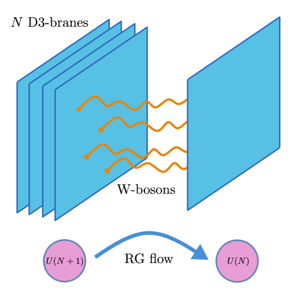
Figure 3: A sketch of the RG flow triggered by Higgsing the $U(N+1)$ gauge theory to $U(N)$, along with its bulk counterpart with separated D3-branes connected by W-bosons.

In [82, 83, 84, 85], the authors describe and conjecture various features of the putative deformation that implements the flow driven by Higgsing. Since the bare Lagrangian does not change, while the vacuum does, this deformation ought to arise integrating out the massive W-bosons corresponding to open strings stretching between the branes. In order to keep these modes in the theory, the correct decoupling limit is argued in [85] to be slightly different than usual. The dual operator $\mathcal{O}_{8}$ is argued to be the (supersymmetric completion of the) first Born-Infeld correction to the Yang-Mills Lagrangian (see [86] for more details),

$$\mathcal{O}_{8}=\mathcal{Q}^{4}\overline{\mathcal{Q}}^{4}\,\text{Tr}X^{4}\propto\text{Str}\left(F^{4}-\frac{1}{4}\,(F^{2})^{2}\right)+\dots{}$$ (5.1)

and it is argued that its dimension is exactly 8. Therefore, the corresponding coupling $h$ has dimension exactly -4 along the RG flow, which connects two superconformal fixed points breaking half of the supersymmetries (just like separating branes in the bulk does with respect to the near-horizon limit). The gauge-coupling beta function vanishes, and the anomalous dimension is therefore exact. The beta function of the $h$ coupling (defined by $\Delta\mathcal{L}=h\frac{\mathcal{O}_{8}}{\Lambda_{4}}$) is thus $\beta_{h}\sim 4h$, so that $h\sim h_{0}\,e^{-4t}$ as a function of the RG time $t\equiv\log\frac{\Lambda}{\mu}$ in the infrared (IR) part of the flow $t\gg 1$, where the deformation operator is irrelevant and described by eq. 5.2.

In order to evaluate the (asymptotic) distance along the RG flow, we need the two-point correlator of the deformation operators. In [87] it was argued that the properly normalized correlator, namely the one associated to the usual Lagrangian $\mathcal{L}_{\text{SYM}}=-\frac{1}{4g_{\text{YM}}^{2}}\text{Tr}F^{2}+\dots$, at the superconformal fixed point

$$\langle\mathcal{O}_{8}(x)\mathcal{O}_{8}(0)\rangle\propto\frac{N^{0}\,\lambda^{4}}{\absolutevalue{x}^{16}}$$ (5.2)

does not scale with $N$ in the ’t Hooft limit. The quantum information metric tensor is essentially a matrix of two-point correlators, for instance the prescription of [43] defines

$$g_{ab}=\int d^{4}x\,\langle\partial_{a}\mathcal{L}(x)\,\partial_{b}\mathcal{L}(0)\rangle$$ (5.3)

for Lagrangians linear in the couplings $\lambda^{a}$. When pulled back along the RG flow, the metric depends on the energy-momentum trace $\Theta(x)=\beta_{h}\,\mathcal{O}(x)$, and one thus finds

$$ds^{2}\overset{\text{IR}}{\sim}e^{-8t}\,dt^{2}$$ (5.4)

up to a prefactor of order $N^{0}$. The information distance is thus finite and of order $N^{0}$ across a single RG step $N\to N\pm 1$.

In order to build the correctly normalized bulk distance, one ought to divide by

$$(L_{\text{AdS}}M_{\text{Pl}})^{\frac{3}{2}}=\sqrt{C_{T}(N)}\propto N\,.$$ (5.5)

All in all, the distance across one step is proportional to $1/N$, and therefore the total bulk distance

$$\Delta(N_{1},N_{2})\sim\sum_{n=N_{1}}^{N_{2}}\frac{1}{\sqrt{C_{T}(n)}}\sim\log\frac{N_{2}}{N_{1}}\,.$$ (5.6)

This is precisely the scaling predicted by the AdS distance conjecture, since the light Kaluza-Klein modes associated to the internal $S^{5}$ have masses that scale with powers of $N$ and thus decay exponentially in the properly normalized distance. Let us stress that this computation has the limitation of only including the IR contribution to the RG length of each step in the chain, where one has computational control. However, nothing seems to depend on $N$ prior to the normalization in eq. 5.6. Hence, integrating along the whole flow should not change the asymptotics which we obtain.

Another observation along the lines of [40] is that $N=1$ does not seem to lie at infinite distance. This resonates with the idea that, since $U(1)$ SYM is a genuinely interacting CFT, it has no tower of conserved higher-spin currents. Had this not been the case, light higher-spin excitations would have had to replace the absent Kaluza-Klein modes in this regime [24, 26, 25], but since there are none the distance cannot be finite on account of the emergent string proposal.

5.1.1 Another large-$N$ limit

The above computation is carried out in the ’t Hooft limit, where $N\gg 1$ with $\lambda\equiv g_{\text{YM}}^{2}N=g_{s}N$ is kept fixed. However, one may object that we really should move along the values of $N$ without deforming any marginal couplings. Let us now analyze this case. Letting $k_{8}$ be the normalization of the correlator

$$\langle\mathcal{O}_{8}(x)\mathcal{O}_{8}(0)\rangle=\frac{k_{8}}{\absolutevalue{x}^{16}}$$ (5.7)

at the (IR) superconformal fixed point, the line element along the RG flow in the deep IR, where this expression is expected to be reliable, is proportional to $ds\overset{\text{IR}}{\sim}k_{8}\,h_{0}\,e^{-4t}\,dt$. In [88, 85, 89] it is argued that $k_{8}\propto\lambda^{4}$ which now scales as $N^{4}$ while the $\mathcal{O}(1)$ coefficient $h_{0}\propto\frac{R_{\text{sep}}^{4}}{\delta^{4}}$ depends on the AdS radius associated to the separated brane stack, something of order $N^{0}$ in our limit, and on the distance $\delta$ between the brane stacks.

In [88] the authors describes a special scale, called gravitational gap, given by $m_{g}\propto m_{\text{W}}/\sqrt{\lambda}$, where $m_{W}=g_{\text{YM}}\,\delta/\alpha^{\prime}$ is the W-boson mass. Analyzing the holographic matching to the low-energy bulk EFT, the authors of [88] conclude that $m_{g}$ is the physical UV cutoff of the EFT. If that is the case, the spacetime integral in eq. 5.3 is cut off at $m_{g}$ instead of $\Lambda$ (which may be taken to be $m_{\text{W}}$), bringing along a factor of $m_{g}^{4}/m_{\text{W}}^{4}=\lambda^{-2}$ that cancels the dependence on $N$. As a result, the total bulk distance is again logarithmic. This effect is somewhat reminiscent of how the quantum gravity cutoff in the presence of parametrically many light species scales differently, but it is not clear whether a deeper connection with this result exists, especially since the standard dictionary uses the ’t Hooft limit.

5.2 Bulk perspective: separated D3-branes

Let us now see what happens in the bulk dual of our $\mathcal{N}=4$ setup, namely the backreacted supergravity geometry produced by the D3-branes. This setting is particularly convenient, since the domain wall solutions we are interested in stem from ten-dimensional type IIB geometries that in the Einstein frame take the form

$$ds^{2}_{10}=H^{-1/2}\,dx_{3,1}^{2}+H^{1/2}\,dy_{6}^{2}\,,$$ (5.8)

where the transverse harmonic function (we omit the +1 in the near-horizon limit)

$$H(Y)=R^{4}\,\int d^{6}y\,\frac{\sigma(y)}{\absolutevalue{Y-y}^{4}}$$ (5.9)

describes the distribution of D3-branes, with $R^{4}\propto\lambda$ the near-horizon AdS radius, so that $\int d^{6}y\,\sigma(y)=1$. For general $\sigma$ the relation between the ten-dimensional solution and the 42 (gauged) supergravity scalars in five dimensions is very complicated, and appears to be only known for in a few special cases. However, for $SO(6)$-symmetric geometries only the radion $\rho$ is excited: writing

$$dy_{6}^{2}=dr^{2}+r^{2}\,d\Omega^{2}_{5}\,,$$ (5.10)

for $H=H(r)$ the only modulus that is excited is the overall volume of the sphere. Therefore, since also the dilaton does not vary along a domain wall transition, the only field that flows is the radion $\rho$, whose kinetic metric is $\frac{d\rho^{2}}{\rho^{2}}$ up to a prefactor.

Starting from $N_{1}$ D3-branes placed at the origin, $N_{1}\,\sigma_{\text{initial}}(y)=N_{1}\,\delta^{(6)}(y)$, separating $N_{1}-N_{2}$ of them by an amount $\Delta$ and smearing them on the sphere gives

$$N_{1}\,\sigma(y)=N_{2}\,\delta^{(6)}(y)+\frac{N_{1}-N_{2}}{\text{Vol}(S^{5})}\,\int_{S^{5}}d\Omega(\hat{\nu})\,\delta^{(6)}(y-\Delta\,\hat{\nu})\,,$$ (5.11)

where the integral is over unit vectors $\hat{\nu}$. This distribution produces a radially symmetric harmonic function $H(r)$ with a 5d geometry that interpolates between $\text{AdS}_{5}(N_{2})$ as $r\to 0$ and $\text{AdS}_{5}(N_{1})$ as $r\to+\infty$.

With this setup, the distance across the DW is simply (up to a pre-factor)

$$\int_{\rho(r=0)}^{\rho(r\to\infty)}\frac{d\rho}{\rho}=\log\frac{\rho(r\to\infty)}{\rho(r=0)}\propto\log\frac{H(r\to\infty)}{H(r\to 0)}=\log\frac{N_{1}}{N_{2}}\,.$$ (5.12)

In this case, one can compute the total distance directly, since in the ’t Hooft limit appropriate for holography the five-dimensional Planck mass does not depend on $N$.

The above computation seems to work for any $SO(6)$-symmetric distribution of branes. In particular, one can use a single domain wall carrying all of the charge or many elementary ones. This seems reasonable, since in this case there is only one flux and thus only one possible path. Perhaps in transitions where many scalars flow the specific distribution of branes will be more important, and there may be an optimal distribution that minimizes the total distance along the lines of eq. 2.5.

5.2.1 Separating without smearing

As we have mentioned, extending the above computation beyond isotropic brane distributions is considerably more difficult, since it involves exciting more of the 42 scalar fields of the underlying five-dimensional gauged supergravity. However, for simple cases such as two separated brane stacks one can still bound the distance and show the relevant logarithmic scaling. This is because many distributions of D3-branes, encoded in eq. 5.9, only excite the diagonal components $\{X_{i}\}_{i=1,\dots,6}$ of the unimodular $6\times 6$ matrix of scalar fields appearing in the ten-dimensional metric [90, 91, 92, 93]. These fields describe deviations from sphericity, while the radion $\rho$ describes the change in volume. Therefore, on account of the discussion in the preceding section, in order to show that the total distance scales logarithmically one only need show that the contribution from the $X_{i}$ is bounded above by a logarithm. The kinetic terms take the form

$$\sum_{i=1}^{6}\frac{(\partial X_{i})^{2}}{X_{i}^{2}}\,,$$ (5.13)

and thus the contribution to the (single-step) distance along the domain wall profile can be bounded above by

$$\Delta_{\text{ss}}^{X}\leq k\,\sum_{i=1}^{6}\log\frac{X_{i}^{\text{max}}}{X_{i}^{0}}\,,$$ (5.14)

where in the vacuum $X_{i}^{0}=1$ by unimodularity and isotropy, up to an irrelevant $\mathcal{O}(1)$ constant $k$.

In order to see that the maximum value $X_{i}^{\text{max}}$ attained by the anisotropy fields scales at most as a power of $N$, we consider the simple case of two parallel brane stacks, without smearing. The corresponding harmonic function in eq. 5.9 is given by

$$N_{1}\,\sigma(y)=N_{2}\,\delta^{(6)}(y)+(N_{1}-N_{2})\,\delta^{(6)}(y-\Delta\,\hat{\nu})\,,$$ (5.15)

where without loss of generality we choose the direction $y\cdot\hat{\nu}=y_{1}$. The corresponding expression for $H$ depends separately on $y_{1}$ and $Y^{2}\equiv y^{2}-y_{1}^{2}$. As a result of this choice of preferred direction, $X_{i}=X_{2}$ for $i>1$, so that enforcing unimodularity the $X_{i}$ are given by

$$X =\left(X_{1}\,,\,X_{2}\,,\,X_{2}\,,\,X_{2}\,,\,X_{2}\,,\,X_{2}\right)$$ (5.16)

$$=(h_{1}\,h_{2}^{5})^{\frac{1}{6}}\left(\frac{1}{h_{1}}\,,\,\frac{1}{h_{2}}\,,\,\frac{1}{h_{2}}\,,\,\frac{1}{h_{2}}\,,\,\frac{1}{h_{2}}\,,\,\frac{1}{h_{2}}\right)\,,$$

following primarily the notation of [93]. These fields appear in the harmonic function $H$ that defines the metric, to be matched to eq. 5.9. In order to match the two, one has to choose a coordinate system where the transverse space metric is the Euclidean $dy_{6}^{2}$ of eq. 5.8. This can be done as in [93], passing from the conventional coordinates $\mu^{i}$ of [90, 91, 92, 93] (subject to $\sum_{i}\mu^{i}\mu^{i}=1$) to the Cartesian coordinates $y^{i}=\sqrt{h_{i}}\,\mu^{i}$ in

$$\frac{1}{H}=(h_{1}h_{2}^{5})^{\frac{1}{2}}\sum_{i}\frac{(\mu^{i})^{2}}{h_{i}}$$ (5.17)

The resulting expression for $H$ is a rational function of $y_{1}^{2}\,,\,Y^{2}\,,\,h_{1}\,,\,h_{2}$, and the constraint

$$\frac{y_{1}^{2}}{h_{1}}+\frac{Y^{2}}{h_{2}}=1$$ (5.18)

can be solved to eliminate $h_{1}$ or $h_{2}$ and simplify it. In the isotropic case $h_{1}=h_{2}$ one recovers the familiar $H=(y_{1}^{2}+Y^{2})^{-2}$, in units of the radius $R$ of the $S^{5}$. In the anisotropic case it is difficult to obtain an explicit expression for $h_{1}$ and $h_{2}$, but in the large-$N$ limit we are interested in the harmonic function $H$ for the single-step flow of eq. 5.15 can be written in terms of $\epsilon\equiv\frac{N_{1}-N_{2}}{N_{1}}\ll 1$. For $\epsilon=0$ one recovers the isotropic result, and thus by analyticity matching the structure of eq. 5.17 to eq. 5.9 via eq. 5.15 shows that

$$h_{1}=h_{2}+\epsilon^{\gamma}\,\delta h_{1}+\dots{}$$ (5.19)

for some $\gamma\geq 1$. Generically $\gamma=1$, but it could be larger if the coefficient of the linear correction vanishes. Correspondingly, one also has $X_{i}^{\text{max}}\sim X_{i}^{0}+\epsilon^{\gamma}\,\delta X_{i}$ for some $\gamma\geq 1$. Thus, the contribution of anisotropy to the single-step distance in eq. 5.14 cannot be parametrically larger than the contribution from the radion in eq. 5.12, which also bounds the total single-step distance from below. All in all, the scaling of the discrete distance remains logarithmic, although computing the precise $\mathcal{O}(1)$ prefactor is more difficult in this less symmetric case. The above reasoning was kept quite general because it can be easily generalized to other distributions of branes, isolating the anisotropy contribution proportional to $\frac{N_{1}-N_{2}}{N_{1}}$.

6 Conclusions

We have introduced a notion of distance for discrete landscapes of vacua which takes into account their isolated nature. The idea is based on transitions between vacua mediated by domain walls (or vacuum bubbles in the metastable case).

While difficult to compute in general, it seems that many top-down settings arising from string compactifications afford simple bounds that are compatible with a logarithmic scaling. This pattern points to the idea of a discrete distance conjecture, whereby towers of species at large (discrete) distances become light exponentially fast with respect to this distance. On general grounds, obtaining bounds that are both sharp and useful is difficult due to how the distance is defined, but we have provided some estimates that may describe it qualitatively, at least in the context of BPS domain walls in supergravity.

Starting from a theory with a moduli space which satisfies the ordinary distance conjecture and lifting its moduli space to a discrete set of isolated vacua, one may wonder whether the persistence of exponential decay with respect to the discrete distance induced by domain walls is a swampland condition. If so, such a criterion would be verifiable entirely within the EFT landscape and applicable to EFTs with no moduli, both reasons which make this proposal attractive from a pragmatical perspective. It is conceivable that some EFTs satisfying the former distance conjecture but not the latter exist, but more exploration is needed to understand whether such theories, if any, are inconsistent, and why. Perhaps a first indication to an answer is that simple examples from string theory seem to satisfy this criterion due to hyperbolic field spaces with particular polynomial scalings, although one can construct toy models which also have this property.

To the extent that generalizing from conformal manifolds to RG flows is sensible, the holographic matching that we discussed in section 5 is compelling and seems to support this view, and if further developed it can provide another tool to test proposals for holographic dual CFTs to gravitational EFTs with no known string theoretical construction. Hopefully, the first steps laid out in this paper can be useful to investigate these issues further.

References

- [1] Cumrun Vafa “The String landscape and the swampland”, 2005 arXiv:hep-th/0509212
- [2] T. Daniel Brennan, Federico Carta and Cumrun Vafa “The String Landscape, the Swampland, and the Missing Corner” In Proceedings, Theoretical Advanced Study Institute in Elementary Particle Physics: Physics at the Fundamental Frontier (TASI 2017): Boulder, CO, USA, June 5-30, 2017 TASI2017, 2017, pp. 015 DOI: 10.22323/1.305.0015
- [3] Eran Palti “The Swampland: Introduction and Review” In Fortsch. Phys. 67.6, 2019, pp. 1900037 DOI: 10.1002/prop.201900037
- [4] Marieke Beest, José Calderón-Infante, Delaram Mirfendereski and Irene Valenzuela “Lectures on the Swampland Program in String Compactifications” In Phys. Rept. 989, 2022, pp. 1–50 DOI: 10.1016/j.physrep.2022.09.002
- [5] Mariana Graña and Alvaro Herráez “The Swampland Conjectures: A Bridge from Quantum Gravity to Particle Physics” In Universe 7.8, 2021, pp. 273 DOI: 10.3390/universe7080273
- [6] Nathan Benjamin Agmon, Alek Bedroya, Monica Jinwoo Kang and Cumrun Vafa “Lectures on the string landscape and the Swampland”, 2022 arXiv:2212.06187 [hep-th]
- [7] Hirosi Ooguri and Cumrun Vafa “On the Geometry of the String Landscape and the Swampland” In Nucl. Phys. B 766, 2007, pp. 21–33 DOI: 10.1016/j.nuclphysb.2006.10.033
- [8] Florent Baume and Eran Palti “Backreacted Axion Field Ranges in String Theory” In JHEP 08, 2016, pp. 043 DOI: 10.1007/JHEP08(2016)043
- [9] Daniel Klaewer and Eran Palti “Super-Planckian Spatial Field Variations and Quantum Gravity” In JHEP 01, 2017, pp. 088 DOI: 10.1007/JHEP01(2017)088
- [10] Ralph Blumenhagen, Daniel Kläwer, Lorenz Schlechter and Florian Wolf “The Refined Swampland Distance Conjecture in Calabi-Yau Moduli Spaces” In JHEP 06, 2018, pp. 052 DOI: 10.1007/JHEP06(2018)052
- [11] Ben Heidenreich, Matthew Reece and Tom Rudelius “Emergence of Weak Coupling at Large Distance in Quantum Gravity” In Phys. Rev. Lett. 121.5, 2018, pp. 051601 DOI: 10.1103/PhysRevLett.121.051601
- [12] Florent Baume and José Calderón Infante “Tackling the SDC in AdS with CFTs” In JHEP 08, 2021, pp. 057 DOI: 10.1007/JHEP08(2021)057
- [13] Eric Perlmutter, Leonardo Rastelli, Cumrun Vafa and Irene Valenzuela “A CFT distance conjecture” In JHEP 10, 2021, pp. 070 DOI: 10.1007/JHEP10(2021)070
- [14] Thomas W. Grimm, Stefano Lanza and Chongchuo Li “Tameness, Strings, and the Distance Conjecture” In JHEP 09, 2022, pp. 149 DOI: 10.1007/JHEP09(2022)149
- [15] Muldrow Etheredge et al. “Sharpening the Distance Conjecture in diverse dimensions” In JHEP 12, 2022, pp. 114 DOI: 10.1007/JHEP12(2022)114
- [16] Florent Baume and José Calderón-Infante “On Higher-Spin Points and Infinite Distances in Conformal Manifolds”, 2023 arXiv:2305.05693 [hep-th]
- [17] Muldrow Etheredge et al. “Running Decompactification, Sliding Towers, and the Distance Conjecture”, 2023 arXiv:2306.16440 [hep-th]
- [18] José Calderón-Infante, Alberto Castellano, Alvaro Herráez and Luis E. Ibáñez “Entropy Bounds and the Species Scale Distance Conjecture”, 2023 arXiv:2306.16450 [hep-th]
- [19] Niccolò Cribiori, Dieter Lust and Carmine Montella “Species Entropy and Thermodynamics”, 2023 arXiv:2305.10489 [hep-th]
- [20] Marco Scalisi and Irene Valenzuela “Swampland distance conjecture, inflation and -attractors” In JHEP 08, 2019, pp. 160 DOI: 10.1007/JHEP08(2019)160
- [21] Marco Scalisi “Inflation, Higher Spins and the Swampland” In Phys. Lett. B 808, 2020, pp. 135683 DOI: 10.1016/j.physletb.2020.135683
- [22] Miguel Montero, Cumrun Vafa and Irene Valenzuela “The dark dimension and the Swampland” In JHEP 02, 2023, pp. 022 DOI: 10.1007/JHEP02(2023)022
- [23] Luis A. Anchordoqui et al. “The Scale of Supersymmetry Breaking and the Dark Dimension” In JHEP 05, 2023, pp. 060 DOI: 10.1007/JHEP05(2023)060
- [24] Seung-Joo Lee, Wolfgang Lerche and Timo Weigand “Tensionless Strings and the Weak Gravity Conjecture” In JHEP 10, 2018, pp. 164 DOI: 10.1007/JHEP10(2018)164
- [25] Seung-Joo Lee, Wolfgang Lerche and Timo Weigand “Emergent strings, duality and weak coupling limits for two-form fields” In JHEP 02, 2022, pp. 096 DOI: 10.1007/JHEP02(2022)096
- [26] Seung-Joo Lee, Wolfgang Lerche and Timo Weigand “Emergent strings from infinite distance limits” In JHEP 02, 2022, pp. 190 DOI: 10.1007/JHEP02(2022)190
- [27] Stefano Lanza, Fernando Marchesano, Luca Martucci and Irene Valenzuela “Swampland Conjectures for Strings and Membranes” In JHEP 02, 2021, pp. 006 DOI: 10.1007/JHEP02(2021)006
- [28] Stefano Lanza, Fernando Marchesano, Luca Martucci and Irene Valenzuela “The EFT stringy viewpoint on large distances” In JHEP 09, 2021, pp. 197 DOI: 10.1007/JHEP09(2021)197
- [29] Stefano Lanza, Fernando Marchesano, Luca Martucci and Irene Valenzuela “Large Field Distances from EFT strings” In PoS CORFU2021, 2022, pp. 169 DOI: 10.22323/1.406.0169
- [30] Ivano Basile, Andrea Campoleoni, Simon Pekar and Evgeny Skvortsov “Infinite distances in multicritical CFTs and higher-spin holography” In JHEP 03, 2023, pp. 075 DOI: 10.1007/JHEP03(2023)075
- [31] Gary Shiu, Flavio Tonioni, Vincent Van Hemelryck and Thomas Van Riet “AdS scale separation and the distance conjecture” In JHEP 05, 2023, pp. 077 DOI: 10.1007/JHEP05(2023)077
- [32] Oliver DeWolfe, Alexander Giryavets, Shamit Kachru and Washington Taylor “Type IIA moduli stabilization” In JHEP 07, 2005, pp. 066 DOI: 10.1088/1126-6708/2005/07/066
- [33] Rafael Carrasco, Thibaut Coudarchet, Fernando Marchesano and David Prieto “New families of scale separated vacua”, 2023 arXiv:2309.00043 [hep-th]
- [34] Ginevra Buratti, José Calderón and Angel M. Uranga “Transplanckian axion monodromy!?” In JHEP 05, 2019, pp. 176 DOI: 10.1007/JHEP05(2019)176
- [35] Dieter Lüst, Eran Palti and Cumrun Vafa “AdS and the Swampland” In Phys. Lett. B 797, 2019, pp. 134867 DOI: 10.1016/j.physletb.2019.134867
- [36] José Calderón-Infante, Angel M. Uranga and Irene Valenzuela “The Convex Hull Swampland Distance Conjecture and Bounds on Non-geodesics” In JHEP 03, 2021, pp. 299 DOI: 10.1007/JHEP03(2021)299
- [37] Ivano Basile and Stefano Lanza “de Sitter in non-supersymmetric string theories: no-go theorems and brane-worlds” In JHEP 10, 2020, pp. 108 DOI: 10.1007/JHEP10(2020)108
- [38] Davide De Biasio and Dieter Lüst “Geometric Flow Equations for Schwarzschild-AdS Space-Time and Hawking-Page Phase Transition” In Fortsch. Phys. 68.8, 2020, pp. 2000053 DOI: 10.1002/prop.202000053
- [39] John Stout “Infinite Distance Limits and Information Theory”, 2021 arXiv:2106.11313 [hep-th]
- [40] Ivano Basile “Emergent strings at infinite distance with broken supersymmetry”, 2022 arXiv:2201.08851 [hep-th]
- [41] John Stout “Infinite Distances and Factorization”, 2022 arXiv:2208.08444 [hep-th]
- [42] Yixuan Li, Eran Palti and Nicolò Petri “Towards AdS Distances in String Theory”, 2023 arXiv:2306.02026 [hep-th]
- [43] D. J. O’Connor and C. R. Stephens “Geometry, the Renormalization Group and Gravity” In Directions in General Relativity: Papers in Honor of Charles Misner, Volume 1 1, 1993, pp. 272 arXiv:hep-th/9304095 [hep-th]
- [44] Jacob McNamara and Cumrun Vafa “Cobordism Classes and the Swampland”, 2019 arXiv:1909.10355 [hep-th]
- [45] Mirjam Cvetic, Stephen Griffies and Soo-Jong Rey “Static domain walls in N=1 supergravity” In Nucl. Phys. B 381, 1992, pp. 301–328 DOI: 10.1016/0550-3213(92)90649-V
- [46] Mirjam Cvetic, Stephen Griffies and Soo-Jong Rey “Nonperturbative stability of supergravity and superstring vacua” In Nucl. Phys. B 389, 1993, pp. 3–24 DOI: 10.1016/0550-3213(93)90283-U
- [47] Mirjam Cvetic and Stephen Griffies “Domain walls in N=1 supergravity” In International Symposium on Black holes, Membranes, Wormholes and Superstrings, 1992 arXiv:hep-th/9209117
- [48] Mirjam Cvetic, Stephen Griffies and Harald H. Soleng “Local and global gravitational aspects of domain wall space-times” In Phys. Rev. D 48, 1993, pp. 2613–2634 DOI: 10.1103/PhysRevD.48.2613
- [49] Mirjam Cvetic and Harald H. Soleng “Supergravity domain walls” In Phys. Rept. 282, 1997, pp. 159–223 DOI: 10.1016/S0370-1573(96)00035-X
- [50] Anna Ceresole et al. “Domain walls, near-BPS bubbles, and probabilities in the landscape” In Phys. Rev. D 74, 2006, pp. 086010 DOI: 10.1103/PhysRevD.74.086010
- [51] Igor Bandos et al. “Three-forms, dualities and membranes in four-dimensional supergravity” In JHEP 07, 2018, pp. 028 DOI: 10.1007/JHEP07(2018)028
- [52] I. Bandos et al. “Higher Forms and Membranes in 4D Supergravities” In Fortsch. Phys. 67.8-9, 2019, pp. 1910020 DOI: 10.1002/prop.201910020
- [53] Riccardo Antonelli, Ivano Basile and Alessandro Bombini “AdS Vacuum Bubbles, Holography and Dual RG Flows” In Class. Quant. Grav. 36.4, 2019, pp. 045004 DOI: 10.1088/1361-6382/aafef9
- [54] Jewel K. Ghosh, Elias Kiritsis, Francesco Nitti and Lukas T. Witkowski “Revisiting Coleman-de Luccia transitions in the AdS regime using holography” In JHEP 09, 2021, pp. 065 DOI: 10.1007/JHEP09(2021)065
- [55] L. Girardello, M. Petrini, M. Porrati and A. Zaffaroni “Novel local CFT and exact results on perturbations of N=4 superYang Mills from AdS dynamics” In JHEP 12, 1998, pp. 022 DOI: 10.1088/1126-6708/1998/12/022
- [56] L. Girardello, M. Petrini, M. Porrati and A. Zaffaroni “The Supergravity dual of N=1 superYang-Mills theory” In Nucl. Phys. B 569, 2000, pp. 451–469 DOI: 10.1016/S0550-3213(99)00764-6
- [57] D. Z. Freedman, S. S. Gubser, K. Pilch and N. P. Warner “Renormalization group flows from holography supersymmetry and a c theorem” In Adv. Theor. Math. Phys. 3, 1999, pp. 363–417 DOI: 10.4310/ATMP.1999.v3.n2.a7
- [58] Robert C. Myers and Aninda Sinha “Seeing a c-theorem with holography” In Phys. Rev. D 82, 2010, pp. 046006 DOI: 10.1103/PhysRevD.82.046006
- [59] Robert C. Myers and Aninda Sinha “Holographic c-theorems in arbitrary dimensions” In JHEP 01, 2011, pp. 125 DOI: 10.1007/JHEP01(2011)125
- [60] Damiano Anselmi and Dario Buttazzo “Distance Between Quantum Field Theories As A Measure Of Lorentz Violation” In Phys. Rev. D 84, 2011, pp. 036012 DOI: 10.1103/PhysRevD.84.036012
- [61] Damiano Anselmi “Inequalities for trace anomalies, length of the RG flow, distance between the fixed points and irreversibility” In Class. Quant. Grav. 21.1, 2004, pp. 29–50 DOI: 10.1088/0264-9381/21/1/003
- [62] Tristan C. Collins et al. “On Upper Bounds in Dimension Gaps of CFT’s”, 2022 arXiv:2201.03660 [hep-th]
- [63] Severin Lüst, Cumrun Vafa, Max Wiesner and Kai Xu “Holography and the KKLT scenario” In JHEP 10, 2022, pp. 188 DOI: 10.1007/JHEP10(2022)188
- [64] Thomas W. Grimm, Eran Palti and Irene Valenzuela “Infinite Distances in Field Space and Massless Towers of States” In JHEP 08, 2018, pp. 143 DOI: 10.1007/JHEP08(2018)143
- [65] Julian Freigang, Dieter Lust, Guo-En Nian and Marco Scalisi “Cosmic Acceleration and Turns in the Swampland”, 2023 arXiv:2306.17217 [hep-th]
- [66] Pierre Corvilain, Thomas W. Grimm and Irene Valenzuela “The Swampland Distance Conjecture for Kähler moduli” In JHEP 08, 2019, pp. 075 DOI: 10.1007/JHEP08(2019)075
- [67] Thomas W. Grimm and Damian Van De Heisteeg “Infinite Distances and the Axion Weak Gravity Conjecture” In JHEP 03, 2020, pp. 020 DOI: 10.1007/JHEP03(2020)020
- [68] Thomas W. Grimm, Fabian Ruehle and Damian Heisteeg “Classifying Calabi–Yau Threefolds Using Infinite Distance Limits” In Commun. Math. Phys. 382.1, 2021, pp. 239–275 DOI: 10.1007/s00220-021-03972-9
- [69] Thomas W. Grimm, Chongchuo Li and Irene Valenzuela “Asymptotic Flux Compactifications and the Swampland” [Erratum: JHEP 01, 007 (2021)] In JHEP 06, 2020, pp. 009 DOI: 10.1007/JHEP06(2020)009
- [70] Thomas W. Grimm, Erik Plauschinn and Damian Heisteeg “Moduli stabilization in asymptotic flux compactifications” In JHEP 03, 2022, pp. 117 DOI: 10.1007/JHEP03(2022)117
- [71] J. P. Provost and G. Vallee “Riemannian Structure On Manifolds Of Quantum States” In Commun. Math. Phys. 76, 1980, pp. 289–301 DOI: 10.1007/bf02193559
- [72] George Ruppeiner “Riemannian geometry in thermodynamic fluctuation theory” In Rev. Mod. Phys. 67 American Physical Society, 1995, pp. 605–659 DOI: 10.1103/RevModPhys.67.605
- [73] George Ruppeiner “Erratum: Riemannian geometry in thermodynamic fluctuation theory” In Rev. Mod. Phys. 68 American Physical Society, 1996, pp. 313–313 DOI: 10.1103/RevModPhys.68.313
- [74] Reevu Maity, Subhash Mahapatra and Tapobrata Sarkar “Information Geometry and the Renormalization Group” In Phys. Rev. E92.5, 2015, pp. 052101 DOI: 10.1103/PhysRevE.92.052101
- [75] Cédric Bény and Tobias J. Osborne “Information-geometric approach to the renormalization group” In Phys. Rev. A 92.2, 2015, pp. 022330 DOI: 10.1103/PhysRevA.92.022330
- [76] A. B. Zomolodchikov ““Irreversibility” of the flux of the renormalization group in a 2D field theory” In Soviet Journal of Experimental and Theoretical Physics Letters 43, 1986, pp. 730
- [77] Michael Lassig “Geometry of the Renormalization Group With an Application in Two-dimensions” In Nucl. Phys. B334, 1990, pp. 652–668 DOI: 10.1016/0550-3213(90)90316-6
- [78] Brian P. Dolan “A Geometrical interpretation of renormalization group flow” In Int. J. Mod. Phys. A 9, 1994, pp. 1261–1286 DOI: 10.1142/S0217751X94000571
- [79] Brian P. Dolan “Geodesic renormalization group flow” In Int. J. Mod. Phys. A12, 1997, pp. 2413–2424 DOI: 10.1142/S0217751X97001407
- [80] Sayan Kar “The Geometry of RG flows in theory space” In Phys. Rev. D64, 2001, pp. 105017 DOI: 10.1103/PhysRevD.64.105017
- [81] Sayan Kar “Geometry of theory space and RG flows” In The interface of gravitational and quantum realms. Proceedings, 1st Inter-University Centre for Astronomy and Astrophysics Meeting, Pune, India, December 17-21, 2001 A17, 2002, pp. 1037–1046 DOI: 10.1142/S0217732302007089
- [82] Steven S. Gubser and Akikazu Hashimoto “Exact absorption probabilities for the D3-brane” In Commun. Math. Phys. 203, 1999, pp. 325–340 DOI: 10.1007/s002200050614
- [83] Steven S. Gubser, Akikazu Hashimoto, Igor R. Klebanov and Michael Krasnitz “Scalar absorption and the breaking of the world volume conformal invariance” In Nucl. Phys. B 526, 1998, pp. 393–414 DOI: 10.1016/S0550-3213(98)00301-0
- [84] Kenneth A. Intriligator “Maximally supersymmetric RG flows and AdS duality” In Nucl. Phys. B 580, 2000, pp. 99–120 DOI: 10.1016/S0550-3213(99)00803-2
- [85] Miguel S. Costa “A Test of the AdS / CFT duality on the Coulomb branch” [Erratum: Phys.Lett.B 489, 439–439 (2000)] In Phys. Lett. B 482, 2000, pp. 287–292 DOI: 10.1016/S0370-2693(00)00484-6
- [86] Joao Caetano, Wolfger Peelaers and Leonardo Rastelli “Maximally Supersymmetric RG Flows in 4D and Integrability”, 2020 arXiv:2006.04792 [hep-th]
- [87] Hong Liu and Arkady A. Tseytlin “Dilaton - fixed scalar correlators and AdS(5) x S**5 - SYM correspondence” In JHEP 10, 1999, pp. 003 DOI: 10.1088/1126-6708/1999/10/003
- [88] Miguel S. Costa “Absorption by double centered D3-branes and the Coulomb branch of N=4 SYM theory” In JHEP 05, 2000, pp. 041 DOI: 10.1088/1126-6708/2000/05/041
- [89] Leonardo Rastelli and Mark Van Raamsdonk “A Note on dilaton absorption and near infrared D3-brane holography” In JHEP 12, 2000, pp. 005 DOI: 10.1088/1126-6708/2000/12/005
- [90] Mirjam Cvetic, S. S. Gubser, Hong Lu and C. N. Pope “Symmetric potentials of gauged supergravities in diverse dimensions and Coulomb branch of gauge theories” In Phys. Rev. D 62, 2000, pp. 086003 DOI: 10.1103/PhysRevD.62.086003
- [91] Mirjam Cvetic et al. “Consistent SO(6) reduction of type IIB supergravity on S**5” In Nucl. Phys. B 586, 2000, pp. 275–286 DOI: 10.1016/S0550-3213(00)00372-2
- [92] Marika Taylor “Higher dimensional formulation of counterterms”, 2001 arXiv:hep-th/0110142
- [93] Eric Bergshoeff, Mikkel Nielsen and Diederik Roest “The Domain walls of gauged maximal supergravities and their M-theory origin” In JHEP 07, 2004, pp. 006 DOI: 10.1088/1126-6708/2004/07/006