Generating drawdown-realistic financial price paths using path signatures

Abstract

A novel generative machine learning approach for the simulation of sequences of financial price data with drawdowns quantifiably close to empirical data is introduced. Applications such as pricing drawdown insurance options or developing portfolio drawdown control strategies call for a host of drawdown-realistic paths. Historical scenarios may be insufficient to effectively train and backtest the strategy, while standard parametric Monte Carlo does not adequately preserve drawdowns. We advocate a non-parametric Monte Carlo approach combining a variational autoencoder generative model with a drawdown reconstruction loss function. To overcome issues of numerical complexity and non-differentiability, we approximate drawdown as a linear function of the moments of the path, known in the literature as path signatures. We prove the required regularity of drawdown function and consistency of the approximation. Furthermore, we obtain close numerical approximations using linear regression for fractional Brownian and empirical data. We argue that linear combinations of the moments of a path yield a mathematically non-trivial smoothing of the drawdown function, which gives one leeway to simulate drawdown-realistic price paths by including drawdown evaluation metrics in the learning objective. We conclude with numerical experiments on mixed equity, bond, real estate and commodity portfolios and obtain a host of drawdown-realistic paths.

1 Introduction

Market generators are generative machine learning (ML) models with the specificity of modeling financial markets such as stock price or return time series, order books, implied volatility surfaces, and more. They have gained popularity in recent years (Wiese et al. [1], Koshiyama et al. [2], Cont et al. [3], Bergeron et al. [4]). Arguably the main advantage of generative ML over existing simpler solutions such as standard Monte Carlo engines is being able to simulate realistic financial time series without having to specify a data generating process (DGP) a priori. Scenario realisticness relates to low distributional divergences between the actual and generated return distributions (such as difference in normalized moments or max mean discrepancy, entropy or Kullback-Leibler divergence, optimal transport measures like Wasserstein distance, etc.), and distances between their autocorrelation functions and tail indices. Some striking results in the latter regard have been found in Wiese et al. [1], Cont et al. [3], Buehler et al. [5] and Vuletić et al. [6].

A drawdown is a price fall relative to its historical maximum. In this article, we argue that one can use a market generator as a non-parametric Monte Carlo engine in order to solve the difficult problem of generating realistic drawdown scenarios. With parametric DGP approaches, no explicit analytical link between the underlying DGP parameters and their corresponding drawdown distribution is known, unless under very restrictive assumptions. Parametric approaches to drawdown have commonly relied on Brownian assumptions as to use Lévy’s theorem to obtain this analytical drawdown distribution. Especially in applications where this measure is crucial one would need theoretical guarantees that upon convergence of the parameters of the generative model drawdowns are explicitly preserved. Examples include pricing drawdown options for max loss insurance (Carr et al. [7], Atteson and Carr [8]) and controlling for drawdown in a portfolio optimization context (Chekhlov et al. [9], [10]).

The main contribution of this paper is overcoming the issues of non-differentiability and numerical complexity inherent to the drawdown function by approximating it with a linear regression on the path’s signature terms. Signatures serve as the moment generating function on the path space and are because of their universality (Chevyrev and Oberhauser [11]) the likely candidate for universal approximation of drawdown with a linear function. We prove the required regularity of drawdown function and the consistency of the approximation. Furthermore, we discuss the adequacy of the approximation as a function of the approximation order and for different levels of roughness and sample sizes. We argue that by adding weighted moments of the path to the reconstruction loss of the market generator, one can obtain realistic drawdown scenarios, solving the understatement of adverse drawdown scenarios of traditional generative model architectures or common DGP assumptions.

The article is structured as follows. Section 2 covers the background on market generators and positions our problem setting within this literature. Section 3 discusses drawdowns, notations and its Lipschitz continuity following from its reformulation as a non-linear dynamic system. Section 4 summarizes some key elements from rough path theory and the approximation of functions on paths. We propose a linear approximation of drawdowns in the signature space. Section 5 introduces our market generator model and its implementation. Section 6 covers our numerical study with experiments on fractional Brownian and empirical data. Section 7 concludes.

2 Market Generators

This section briefly covers the background on market generators, related papers and their commonalities that lead to the questions posed in this paper.

The potential benefits of generative machine learning for modeling financial time series have been early recognized by Kondratyev and Schwarz [12], Henry-Labordere [13], and Wiese et al. [1], who first applied restricted Boltzmann machines (Smolensky [14]) and generative adversarial networks (Goodfellow et al. [15]) respectively to financial sequences data. Since those papers, a host of use cases have been proposed that include time series forecasting (Wiese et al. [1]), trading strategy backtesting (Koshiyama et al. [2]), hands-off volatility surface modeling (Cont and Vuletić [16]), option pricing and so-called deep hedging (Buehler et al. [5], [17]), and more.

Closest related to this work is the paper of Buehler et al. [5] who also use the combination of variational autoencoder and signatures, with the general aim of reproducing some of the stylized facts of financial time series (Cont [18]). However, they use signatures in the input space and then output signature values, which implies that deploying their model requires a scalable inversion of signatures back to paths, which is far from trivial. Similar to Ni et al. [19] who use signatures in the discriminator of a GAN architecture, the generator in this paper does not output signatures but only uses them in the loss evaluation step. Moreover, much work on market generators has revolved around adjusting the loss function such that desired features of the timeseries are reproduced. This is very close to our proposed approach. Cont et al. [3] evaluate the tail risk (value-at-risk and expected shortfall) of the simulations to evaluate their adequacy. Recently, Vuletić et al. [6] included profit-and-loss (P&L) similarity and Sharpe ratios in the loss function to increase the financial realism of the generated scenarios. This paper builds on top of that. Drawdown is a similar metric that in most financial contexts would be a useful feature to reproduce, because it captures both P&L and autocorrelation, but in fact is in some financial contexts the most important metric, such as portfolio drawdown control, optimization, or drawdown insurance. For instance, some investment strategies or fund managers get automatically closed down if they breach certain drawdown limits and it is thus crucial that a simulation of their strategies does not understate the probability of larger drawdowns. However, as a path functional, rather than a function on a P&L distribution like a tail loss or Sharpe ratio, drawdown is much more difficult to evaluate. That is why we introduce the approximation trick in the next sections.

3 Drawdowns

This section introduces the concept of a drawdown and its notation used throughout the paper. We briefly touch upon how it is usually approached in the literature, the issues for data-driven simulation of drawdowns and the expression of drawdown as a non-linear dynamic system. The latter insight, combined with the concept of a path signature, will allow us to introduce the approximation in the next sections.

3.1 Introduction and notation

The drawdown is the difference at a point in time $t$ between a price $S_{t}$ and its historical maximum up to that point. For a price path (in levels) $S:[0,T]\xrightarrow{}\mathbb{R}$ define drawdown function $\Xi$ as:

$$\xi_{t}=\Xi(S)_{t}=\max(\max_{k<t}(S_{k})-S_{t},0)$$ (1)

We are interested in the distribution $\mathcal{P}(\xi)$ as a function of the DGP parameters of $S$, denoted by $\theta$. It is clear that the drawdown is a non-trivial function of the underlying DGP and captures at least three dimensions. Firstly, the drift or deterministic tendency of achieving a new maximum. Secondly, the dispersion or volatility of $S$, which determines the probability of a loss vis-a-vis this monotonic drift. Thirdly, and not grasped by standard Markovian assumptions, the autocorrelation of losses or the probability that the nonzero drawdown will persist, i.e. the duration of the drawdown. The analytical link between these components or a generalized DGP and the drawdown distribution is unknown and depends on the specific process. In the drawdown literature that uses parametric simulation (e.g. [7][8][20][21]), one often assumes (geometric) Brownian motion and leverages Lévy’s theorem (Lévy [22]), which determines the joint law of the running maximum of a Brownian and the deviation to this maximum, to find the analytical distribution of drawdown as a function of the drift and volatility of the DGP. This yields closed-form expressions of the distribution $\mathcal{P}(\xi)$ (e.g. see Douady et al. [21] and more concisely Rej et al. [20]). However, martingale processes like Brownian motion do not exhibit return autocorrelation and one expects a sequence of consecutive losses to result in larger drawdown scenarios. Goldberg and Mahmoud [23] assume an autoregressive process of order 1 (AR(1)) and show that increasing autocorrelation leads to more extreme drawdowns. Van Hemert et al. [24] introduce drawdown greeks and discuss the sensitivity of the maximum $\xi$ value to the autocorrelation parameter under normal return assumptions and find strong dependence on the assumed level of AR(1) autocorrelation. Hence, standard martingale assumptions only lead to optimistic lower bounds on those worst case drawdown scenarios, as was also emphasized in Rej et al. [20]. Obtaining a simulated $\mathcal{P}(\xi)$ faithful to the empirical drawdown distribution through selecting DGP parameters is thus hard to obtain, as it is very sensitive to serial dependence and the analytical link between $\theta$ and $\mathcal{P}(\xi)$ does not exist except under very restrictive assumptions (cf. [24]). In drawdown papers that use non-parametric simulation (e.g. [9][10][25][24]), the scenarios are limited to the historical sample (e.g. historical blocks in a block bootstrap procedure), which drastically limits available samples. This jeopardizes the convergence of data-hungry models in the non-overlapping block case, and creates multicollinear (or identical) conditions for the overlapping (or oversampled) blocks case. For instance, Chekhlov et al. [10] discuss how multiple scenarios increase the effectiveness of drawdown optimizers over a single historical scenario, but also indicate how oversampling a limited dataset has diminishing returns in terms of out-of-sample risk-adjusted returns of the drawdown optimization strategy. Ideally, one has a vast number of rich drawdown scenarios, but this is limited with historical simulation and an unsolved problem for parametric Monte Carlo. One way to cope with these issues is to simply not embed the parameters that capture drawdown in the DGP, derive its distribution from said DGP assumptions or rely on few, overlapping or identical paths, but to construct a non-parametric simulation approach that relies on learning with flexible mappings rather than calibrating known parameters. We show that one can rather rely on a market generator to abstract both the DGP and the link between DGP and drawdown distribution, and learn to reproduce this distribution in a Monte Carlo. Learning means updating the parameters of an implicit DGP (e.g. the parameters of a neural network), denoted by $\theta$, over batches of training data of $S$ to increasingly improve its ability to reproduce the drawdowns in the synthetic samples, denoted by a parametrized path $S_{\theta}$. This Monte Carlo could be used to devise strategies that control drawdown or as a simulation engine for pricing drawdown insurance in a fully non-parametric way.

3.2 Issues with the drawdown measure for data-driven simulation

The problem with the drawdown measure, compared to simpler measures on the moments of the P&L, is that at first glance it looks unsuited for learning. The reasons are twofold.

• Differentiability: $\Xi$ is non-differentiable w.r.t. a parameterized path $S_{\theta}$. At first glance it looks impossible to change the DGP parameters $\theta$ by including ’feedback’ on $\frac{\delta(\Xi(S_{\theta}))}{\delta(\theta)}$, without making simple assumptions on the specification of $\theta$.

• Complexity: evaluating the maximum of a vector of $n$ numbers takes $n$ operations or $O(n)$. Naively evaluating the running maximum takes $n(n+1)/2$ or $O(n^{2})$ operations. If one would use a smoothed approximation of the maximum (such as smooth normalized exponentials [26] or softmax transformation) to resolve non-differentiability, this would be computationally prohibitive (especially for long $n$ paths). Moreover, accuracy of such naive exponential smoothing would rely on the scale of $S$ and variation around the local maxima.

The main contribution of this paper is that these issues of non-differentiability and numerical complexity can be jointly overcome by approximating the drawdown of a path by using linear regression on its signature terms.

3.3 Drawdown as a non-linear dynamic system and Lipschitz continuity

Assume the price path $S:[0,T]\xrightarrow{}\mathbb{R}$ is a piecewise linear continuous path of bounded variation (e.g. finite variance), such as interpolated daily stock prices, index levels or fund net asset values (NAV). Denote by $\mathcal{V}([0,T],\mathbb{R})$ the (compact) space of all such paths. Firstly, we need to remark that while from (1) we know the max operator makes $\Xi$ not continuously differentiable, the variation in $\Xi$ is bounded by the variation in the paths. When taking two bounded paths the distance between their maximum values is bounded by a norm on the distance between their path values:

$$|\max_{0<i<T}(S^{1}_{i})-\max_{0<j<T}(S^{2}_{j})|\leq\max_{i,j\in[0,T]}|S^{1}_{i}-S^{2}_{j}|=||S^{1}-S^{2}||_{\infty}$$ (2)

where $|.|$ denotes the standard absolute value sign (as an $S_{t}$ is a scalar), while $||.||_{\infty}$ denotes the infinity norm or maximum distance between two paths (as an $S$ is a full path). In words, the distance between two maxima is capped by the maximum distance between any two values on path $S^{1}$ and $S^{2}$. This means that if two paths become arbitrarily close in terms of this distance, their respective maxima will become arbitrarily close. More specifically, the maximum is Lipschitz-$C$ continous, with distance inf-norm and $C=1$. Similar arguments can be made for $\Xi$, i.e. application of the maximum operator and a linear combination of two piecewise linear paths is Lipschitz continuous. In particular, Proposition 3.1 shows that the impact on the drawdown function of a change in the underlying paths is bounded in terms of a defined distance metric (inf-norm).

Proposition 3.1 (Lip-regularity of $\Xi$).

Consider by $\mathcal{V}([0,T],\mathbb{R})$ the space of continuous paths of bounded variation $[0,T]\rightarrow\mathbb{R}$, two paths $S^{1},S^{2}$ $\in\mathcal{V}$ and drawdown function $\Xi(S)_{t}:\mathcal{V}\rightarrow\mathbb{R}=\max_{k\leq t}(S_{k})-S_{t}$. We have the following Lipschitz regularity for inf-norm distance $||.||$ and a regularity constant $C$:

$$||\Xi(S^{1})_{t}-\Xi(S^{2})_{t}||\leq C||S^{1}-S^{2}||$$ (3)

Proof.

$$\begin{split}||\Xi(S^{1})_{t}-\Xi(S^{2})_{t}||=||\max_{i\leq t}(S^{1}_{i})-S^{1}_{t}-\max_{j\leq t}(S^{2}_{j})+S^{2}_{t}||\\ \leq\max_{i,j\in[0,t]}||S^{1}_{i}-S^{2}_{j}||+||S^{2}_{t}-S^{1}_{t}||\leq C||S^{1}-S^{2}||\end{split}$$ (4)

Through triangle inequality, the Lipschitz condition holds for $C$ minimal $2$ and distance metric $||.||_{\infty}$, which concludes the proof. ∎

The difference in drawdown between two paths is thus bounded by the distance between the paths. This means that if two paths become arbitrarily close according to said distance metric, their drawdowns will become arbitrarily close. In this article, we explore what this regularity implies for local approximation.

Observe below the differentials of $\xi$ and $S$ at a specific point in time $t$, i.e. we treat drawdown as a non-linear dynamic system which is unnatural as non-differentiability implies $\frac{d\xi_{t}}{dS_{t}}$ is not a continuous function (e.g. what one would depend on for Taylor series-like local approximations). Consider the following dynamic system (also see [21]):

$$d\xi_{t}=f(\xi_{t},dS_{t})=\left\{\begin{aligned} &-dS_{t},\xi_{t}>0\\ &\max(0,-dS_{t}),\xi_{t}=0\end{aligned}\right.$$ (5)

Depending on the current level of drawdown the effect of a price change is either linear or none, hence the derivatives are path dependent. This conditionality illustrates the non-differentiability of $\Xi$ at a time $t$ and the fact that the differentials $|d\xi_{t}|\leq|dS_{t}|$ are bounded. This observation also provides intuition as to why local approximation is feasible. It does make sense to do an interpolation between linear and zero effects, and because of the boundedness one would not be arbitrarily off. For instance, one could assume linear dynamics but with a stochastic component derived from the average time in drawdown, i.e. the probability of a linear effect. In practice, however, the solution of this stochastic equation would still depend on our estimate of the average time in drawdown and in that sense not resolve the inherent path dependence. Hence, ideally we would express $\xi$ as some function of the vector-valued $S$ (or intervals of $S$), rather than a scalar $S_{t}$ (or increments $dS_{t}$) and treat the path dependence in a more natural way. In the next section, this is exactly what rough path theory allows us to do: solving the types of equations Eq. (5) belongs to, offering strictly non-commutative (thus order or path dependent) solutions to these complex non-linear dynamic systems, allowing for a unique solution for the outputs $\xi_{t}$ given inputs $S$, even if their effects $f$ are not continuously differentiable.

4 Rough path theory and the approximation of functions on paths

This section briefly recapitulates some of the central ideas of rough path theory, path signatures and the approximation of functions on paths. Next, we discuss the signature approximation of drawdown where we consider the drawdown of a path as an approximate linear weighing of the moments of the path. This will offer the foundation for generating weighted signatures in the market generator of Section 5.

4.1 Path signatures

Rough path theory was developed by Terry J. Lyons (Lyons et al. [28], [27], [29]) and concerns solving rough differential equations. Consider the controlled differential equation (Lyons et al. [28], Eq. (2)):

$$dY_{t}=g(Y_{t})dX_{t}$$ (6)

where $X$ is a path of bounded variation, called the driving signal of the dynamic system. $g$ is a mapping called the physics that models the effect of $dX_{t}$ on the response $dY_{t}$. A controlled differential equation distinguishes itself from an ordinary differential equation in that the system is controlled or driven by a path ($dX$) rather than time ($dt$) or a random variable (stochastic differential equation, $d\varepsilon$). Rough path theory considers solution maps for driving signals that are much rougher (highly oscillatory and potentially non-differentiable) than e.g. a linear path of time or a traditional Brownian driving path. It is more robust to consider Eq. (6) over Eq. (5), and replace $dS_{t}$ as an input with its integral. We can rewrite Eq. (5) in this form by setting $Y=\Xi$, $X_{t}=(t,\int_{s=0}^{t}dS_{s}ds)$ and $g(y,(t,x))=f$ (e.g. see Liao et al. [30], Eq. (2)). This allows the effect to be of a broader type and need not even be differentiable for equation (6) to be well defined. The Picard-Lindelöf theorem (Lyons et al. [28], Theorem 1.3) states that if $X$ has bounded variation and $g$ is Lipschitz, then for every initial value $y_{0}$ in the image of $Y$, the differential equation (6) admits a unique solution. Importantly, if the effect of $X$ on $Y$ is not Lipschitz, we lose the uniqueness of the solution. As shown in Appendix Appendix: Controlled differential equations and path signatures, through Picard iteration and under an additional regularity assumption on $g$, one naturally arrives at $M$-step Taylor approximation $\hat{Y}(M)_{t}$ on the path space for the $Y_{t}$ in Eq (6):

$$\hat{Y}(M)_{t}=y_{0}+\sum_{m=1}^{M}g^{\circ m}(y_{0})\underset{u_{1}<...<u_{m},u_{1},...,u_{m}\in[0,T]}{\int...\int}dX_{u_{1}}\otimes...\otimes dX_{u_{m}}$$ (7)

The $m$-fold iterated integral on the right hand side of Eq (7) is called the $m$-th order signature of the path $X$, which we denote by $\Phi^{m}(X)$.

Signatures have useful symmetries and properties, for our use case most notably universality and uniqueness, which we will briefly explain below. For now, we should note that equations of this form admit uniform estimates of $Y$ when $X$ is a rough path (highly oscillatory and non-differentiable), and it suffices to control the variation of the path $X$ (of bounded $p$-variation, such as finite-variance paths) and the regularity of $Y$ (Lyons et al. [28], conditions for Eq. (2) to hold).

Clearly, $\hat{Y}(M)_{t}$ is linear in the truncated signature of $X$ up to order $M$. Moreover, the error bounds of $\hat{Y}(M)_{t}$ to approximate $Y_{t}$ display a factorial decay in terms of $M$:

$$|Y_{t}-\hat{Y}(M)_{t}|\leq C_{\gamma}\frac{|X|^{M+1}_{1,[0,t]}}{M!}$$ (8)

where the rate decay depends on the roughness of the signal, denoted by $\gamma$ [31]. Eq. (7) and (8) aptly summarize the signature’s universality, i.e. a non-linear $Y$ on $X$ can be well approximated by a linear function $L$ on $\Phi^{m}(X)$.

For instance, if one replaces the path $X$ by scalar $x$ and thus non-commutative tensor products $\otimes$ become simple products, the $m$-times repeated integral on $dx$ is $\frac{x^{m}}{m!}$ which is the classical exponential series we know from a standard Taylor expansion. Signatures are thus the monomials of the path space (Lyons [27]), the generalization of local approximation to functions of paths by offering a strictly non-commutative exponential function.

Chevyrev and Oberhauser [11] introduce signatures as the moment generating function on the path space, as they play a similar role to normalized moments for path-valued data instead of scalar-valued data. This is the uniqueness property: paths with identical signatures are identical in the distributional sense as are scalars with the same sequence of normalized moments.

Proof of signature universal non-linearity is due to Lemercier et al. [32] (also see Lyons and McLeod [29] for a more recent redefinition of the result in Theorem 3.4) who prove that for a Lipschitz continous $h$, path of bounded variation $X$, there exist a vector of linear weights $L$ such that for any small $\epsilon$:

$$|h(X)-\langle L,\Phi(X)\rangle|\leq\epsilon$$ (9)

where $\langle x_{1},x_{2}\rangle$ denotes the standard inner product between vectors $x_{1}$ and $x_{2}$, and $\Phi(X)$ the infinite $M$ signature or infinite collection of iterated integrals of a path. By the Stone-Weierstrass theorem (a crucial theorem in proving the universal approximation capabilities of neural networks, Cotter [33] and Hornik [34]) it is proven that signatures are a universal basis in the sense that they allow us to express non-linear path functions $h$ as a linear function of signatures $\Phi(X)$ provided that they have the required regularity. As for classical Taylor series, although a function might not be $k$-times differentiable, a high order smooth polynomial approximation can be a quantifiably close (bounded error) approximation for bounded Lipschitz functions, provided $C$ is small. In this paper, we apply this common insight to path functions, and drawdowns in particular.

4.2 Signature approximation of drawdown

We noted in Section 3 that drawdown is a non-linear, non-differentiable function of its underlying path $S_{\theta}$, which is smooth in the bounded differentials $d\xi/dS$ sense. Its outcome can be seen as an interpolation between two types of path dependent effects. In this section, we leverage the boundedness of Section 3 together with the universality of signatures of Section 4 to introduce a smooth local approximation by linear approximation of drawdown on path signatures.

We propose an approximation $\hat{\xi}(M)_{t}$ of $\xi_{t}$ of the form:

$$\hat{\xi}(M)_{t}=\xi_{0}+\sum_{m=1}^{M}L_{m}\underbrace{\underset{u_{1}<...<u_{m},u_{1},...,u_{m}\in[0,t]}{\int...\int}dS_{u_{1}}\otimes...\otimes dS_{u_{m}}}_{\Phi^{m}(S)}$$ (10)

where $L_{m}$ is a vector of linear coefficients linking the drawdown at $t$ with the signature terms of order $m$ of the path $S$ up to $t$. As per above, $L$ could be considered the iterated effects of intervals up to $t$ on the resulting drawdown $\xi_{t}$, where the coefficients are not the $m$-th order derivatives as they are not defined, but polynomial approximations that are essentially numerical interpolations of the nested effects. Signatures thus offer a strictly non-commutative alternative to the polynomials Taylor series would suggest.

Importantly, for this integration to make sense the path $S$ has to be continuous, hence in practice augmented from discrete observations into the continuous domain by time-augmenting the path. This means adding time as an axis and assuming piecewise linear paths. Other options such as lead-lag and rectilinear augmentation exist (see Lyons and McLeod [29]), but are not favored for this application and may add dimensionality to the paths which increases the number of signature terms per level $M$ and related compute time.

As the ordered iterated integrals represent the drift, Levy area, and higher order moments of the path distribution (see Chevyrev and Oberhauser [11]), Eq. (10 ) thus argues that drawdown can be approximated as a linear function of the moments of the path. Leveraging factorial decay of the approximation error for Lipschitz functions, we argue with Proposition (3.1) and Eq. (5) that with the full signature $M\xrightarrow{}\infty$ one gets an arbitrarily close approximation of $\xi$, where the rate decay depends on the roughness, denoted by $\gamma$, of the underlying price process $S$ (see proofs in Boedihardjo et al. [31]).

In the more compact inner product notation, we propose to apply Eq. (9) to drawdown:

$$|\Xi(S)-\langle L,\Phi(S)\rangle|\leq\mu$$ (11)

where the arbitrary precision $\mu$ is only in theory, because in practice we rely on the truncated signatures of level $M$ as the full signature is an infinite collection, and thus there will be an error $\kappa$ that due to the ordered nature of the coefficients decays factorially in $M$ (e.g. Eq. 8 for the intuition and Boedihardjo et al. [31] for the proofs):

$$\begin{split}\Xi(S)=\langle\hat{L},\Phi^{M}(S)\rangle+\kappa_{M}\end{split}$$ (12)

$$\hat{\Xi}_{M}(S)=\langle\hat{L},\Phi^{M}(S)\rangle$$ (13)

where $\hat{L}$ are the estimated coefficients for a chosen signature truncation level $M$, contrasting the theoretical infinite collection of weights $L$. Similarly, $\hat{\Xi}_{M}(S)$ is the approximated drawdown for this truncation level $M$, while $\Xi(S)$ is the exact value. Note that one could also do an equivalent truncation of the number of linear coefficients $len(\hat{L})$ rather than the signature order. However, from Eq. (10) we know that it is more natural to choose a set of linear coefficients that corresponds to a number of signature terms following the choice of M.

Proposition 4.1 looks into the consistency behaviour of $\kappa$ with respect to a sample size of $K$ sample paths drawn from $\mathcal{V}$ and next we highlight small sample properties that become apparent from the proof.

Proposition 4.1 (Consistency of linear $\mathbf{\Xi(S)}$ approximation on signatures $\mathbf{\Phi^{M}(S)}$).

Consider by $\mathcal{V}([0,T],\mathbb{R})$ the space of continuous paths of bounded variation $[0,T]\rightarrow\mathbb{R}$, $\mathcal{K}\subset\mathcal{V}$ is a compact subset comprising sample paths $S_{k}$, $k\in[0,...,K]$, and $\Xi:\mathcal{V}\rightarrow\mathbb{R}$ is the Lip continuous drawdown function. The approximation error $\kappa$ of $\Xi(S)$ for any $S$ in $\mathcal{V}$ by $\hat{\Xi}(S)$ is bounded through the regularity of $\Xi$ (Proposition 3.1) and the distance in the signature space between $S$ and any $S_{k}$, such that for $K\rightarrow\infty$, $\kappa\rightarrow 0$, or

$$|\Xi(S)-\hat{\Xi}(S)|\rightarrow 0,\textnormal{ for }K\rightarrow\infty$$ (14)

Proof.

Universal nonlinearity of signatures (Eq. 9) is due to Theorem 2.1 in Lemercier et al. [32] and states that for defined $\mathcal{V}$ and $\mathcal{K}$ there exists a truncation level $M\in\mathbb{N}$ and coefficients $\hat{L}$ such that for every $S_{k}\in\mathcal{K}$ we have that for any $\iota$

$$|\Xi(S_{k})-\langle\hat{L},\Phi^{M}(S_{k})\rangle|\leq\iota$$ (15)

We decompose $\kappa=|\Xi(S)-\hat{\Xi}(S)|$ with a triangle inequality as suggested by Eq. (3.6) in Lyons and McLeod [29]:

$$|\Xi(S)-\hat{\Xi}(S)|\leq|\Xi(S)-\Xi(S_{k})|+$$ (16)

$$|\Xi(S_{k})-\hat{\Xi}(S_{k})|+|\hat{\Xi}(S_{k})-\hat{\Xi}(S)|$$ (17)

$$=\textbf{A}_{K}+\textbf{B}_{M(K)}+\textbf{C}_{K}$$ (18)

This inequality bounds the error by the regularity of $\Xi$ in A, the $\iota$ of Eq. (15) in B and a signature distance in C.

By Proposition 3.1, we find that $\textbf{A}\leq C||S-S_{k}||_{\infty}$. For any $k\in[1,...,K]$ with $K\rightarrow\infty$ and the compactness of $\mathcal{V}$ there exists a $k$ such that $||S-S_{k}||_{\infty}\rightarrow 0$ such that A can be reduced to zero. By Eq. (15), $\textbf{B}\leq\iota$, such that this term is governed by the rate decay of Eq. (8). Eq. (15) guarantees we can pick an $M$ high enough such that through Eq. (8), $\iota\leq C_{\gamma}\frac{|S|^{M+1}_{1,[0,T]}}{M!}$ such that this term can be shrunk arbitrarily small as $M$ can be set arbitrarily large for $K\rightarrow\infty$.

As per Eq. (3.7) in Lyons and McLeod [29] the difference between the approximated drawdown of two paths can be bounded by a linear combination of the difference in signatures:

$$\textbf{C}\leq|\langle L,|\Phi^{M}(S_{k})-\Phi^{M}(S)|\rangle|$$ (19)

for an appropriate choice of rough path distance metric [29]. For any $k\in[1,...,K]$ with $K\rightarrow\infty$ and the compactness of $\mathcal{V}$ there again exists a $k$ such that $|\Phi^{M}(S_{k})-\Phi^{M}(S)|\rightarrow 0$ such that C could be reduced to zero, which concludes the proof. ∎

In sum, $\kappa$ converges to zero for $K\rightarrow\infty$ provided that Proposition (3.1) holds for A, while compactness of $\mathcal{V}$ (B and C) is a reasonable assumption in practice.

For finite $K$, we can still use the decomposition in the proof to do error analysis. The drawdown approximation will generalize well as far as (A) the maximum distance between available samples $S_{k}$ and possible new samples in $\mathcal{V}$ is small, (B) the signature truncation level $M$ is chosen appropriately high for the given roughness of the process to let $\iota$ be small enough, (C) as per (A) the distance between the signatures of observed and unobserved paths is small such that term $\mathbf{C}$ is small.

Finally, a remaining modelling choice is the specific choice of $L$. As the approximation is essentially linear, Eq. (12) can be estimated using linear regression (OLS) and higher order polynomials are not required (as one would need to do with e.g. logsignature regression [29]). However, since in practice the sample $K$ is limited and the number of signature terms scales exponentially with $M$, one has to be mindful of overfitting on a limited sample size $K$, e.g. $len(\Phi^{M})>K$. Therefore, we study the impact of regularized linear regression of $\Xi(S)$ on $\Phi^{M}(S)$ with a penalty for the number (absolute shrinkage or selection) and size (proportional shrinkage) of estimated coefficients (i.e. the elastic net (ElNet) regression). We conclude by specifying:

$$\hat{L}=\min_{L}(||\Xi(S)-\langle L,\Phi^{M}(S)\rangle||_{2}+\lambda_{1}||L||_{1}+\lambda_{2}||L||_{2})$$ (20)

$$\hat{\Xi}_{M}(S)=\langle\hat{L},\Phi^{M}(S)\rangle$$ (21)

where $\lambda_{1}=\lambda_{2}=0$ corresponds to OLS, $\lambda_{1}=0$ corresponds to Ridge and $\lambda_{2}=0$ to LASSO regression [35]. In applications below, we set $\lambda_{1}$ and $\lambda_{2}$ using 10-fold cross-validation (CV), such that we can further refer to Eq. (20) as ElNetCV.

5 The model

5.1 Introduction

In this section, we introduce and motivate our generative ML model. The aim of the drawdown market generator, from here on named the $\xi$-VAE, is that upon convergence of (train and validation) reconstruction loss terms we have guarantees that the synthetic samples have preserved the drawdown distribution of the original samples. This is generally not the case in market generator models or financial DGPs with standard martingale assumptions (as per Section 3).

Crafting a DGP to obtain a certain level of drift, volatility or higher order moments is mathematically more straightforward, as those are typically the equations that constitute the DGP. With measures on the P&L, such as value-at-risk (VaR) or expected shortfall (ES) (Cont et al. [3]), one can leverage the direct analytical link between quantiles and moments (e.g. Boudt et al. [36]). As per Section 3, one can express the drawdown distribution as a function of the moments of the static P&L described by the DGP as well, but only under very restrictive assumptions (e.g. Douady et al. [21] and Rej et al. [20]). Besides, one would expect drawdown to be a function of the moments of the path (vector-valued) $S$, rather than the (scalar-valued) $S_{t}$.

In this article, we proposed to approximate drawdown as a linear combination of the moments of the path, as Chevyrev and Oberhauser [11]) define signatures as the moments of the path. As an analogue to quantiles and static moments, we can evaluate these path moments and weigh them according to their importance to simulate realistic drawdowns. Moreover, this approximation implies a smoothing of the drawdown function by the change of basis. The signature is a non-parametric sum of path values. Weighted sums are differentiable. Indeed, because of linearity the loadings of drawdown to signature terms can also be seen as the sensitivities of a path’s drawdown to changing signatures.

Measuring the divergence between the moments of a path by means of a maximum mean discrepancy (MMD) was proposed by Buehler et al. [5]. We essentially add that it is useful to weigh these moments according to the $L$ from Eq. (20) to minimize (and control for) the drawdown divergence between the input and the output samples during training (and validation) epochs. This has the advantages of (1) not requiring signatures in the input or output space, only as part of the objective, and (2) having an explicit drawdown term in the reconstruction loss that allows one to monitor its convergence during training and validation. The next subsection will make this motivation specific and introduce the algorithm.

5.2 The algorithm

Variational autoencoders

The core of our algorithm is a variational autoencoder (VAE), which is a general generative machine learning architecture that links an encoder and decoder neural network in order to generate new samples from a noisy, in this case Gaussian, latent space. The idea of a Monte Carlo is to transform noise into samples that are indistinguishable from the actual samples by scaling them, adding drift, etc. In other words, the neural network that constitutes the decoder is our non-parametric DGP. It does contain the parameters of the neural network, but it is non-parametric in the sense that we do not have to specify the dynamics in a handcrafted formula before we can do Monte Carlo. We rather rely on the universal approximation theorems behind even shallow neural networks (Hornik [34] and Cotter [33]) to approximate a realistic DGP by iterating data through the network and updating the parameters $\theta$ with feedback on the drawdown distribution of the batch, assuring that the approximated DGP converges in train and validation loss to the empirical DGP.

We will not discuss the VAE architecture in depth here, but include an architectural overview in Appendix Appendix 2: Variational Autoencoders and refer the interested reader to Kingma and Welling [38] for details on the encoder and decoder networks $g$, backpropagation, the latent Kullback-Leibler $\mathcal{L}_{L}$ loss and the standard $L2$ reconstruction loss $\mathcal{L}_{R}$.

We should stress here that the main reason for picking a rather standard VAE (over restricted Boltzmann machines, generative adversarial networks, generative moment matching networks or normalizing flow-based VAEs) is their simplicity, speed, flexibility, scalability and stability during training. Boltzmann machines are very efficient to train, but the energy-based loss function and their binary values makes them very inflexible for adjusting objective functions. Through the discriminator mechanism GANs are most flexible and a very popular choice in related literature, but notoriously expensive to train in terms of required data and speed, and associated instabilities such as mode collapse and vanishing gradients leading to subpar results (Eckerli and Osterrieder [39]).

Algorithm 1 Training $\xi$-VAE

Input Historical price paths $S:[0,T]\rightarrow\mathbb{R}$, hyperparameters (listed in Appendix Appendix 2: Variational Autoencoders), signature truncation level M and feature weight $\alpha$.
      Output Trained VAE Market Generator $g_{\theta}$

1:procedure Train

2:    

Divide historical sample into blocks (index $b$, $b\in[1,T-\tau]$) of length $\tau$, calculate the signatures of these paths truncated at level $M$, $\Phi^{M}(S_{b})$, calculate the drawdowns $\Xi$ of these paths $\Xi(S_{b})_{\tau}=\int_{0}^{\tau}(max_{t_{i}<t}(S_{b,{t_{i}}})-S_{b},t)dt$

3:     $\hat{L}\xleftarrow{}ElNetCV({\Xi}(S_{b}),\Phi^{M}(S_{b})$

4:    Initialize the parameters $\theta$ of the VAE.

5:    for $i:\{1,...,N_{t}\}$ do:

6:       

Sample a batch (index $\mathcal{B}$) of blocks and pass it through the encoder $g_{\theta}$ and decoder network $g^{-1}_{\theta}$.

7:       

Calculate drawdown $\Xi(S^{\prime})$ of the output sample $S^{\prime}$ using the differentiable signature approximation: $\langle\hat{L},\Phi^{M}(S^{\prime})\rangle$

8:       

Define the reconstruction loss term as the weighted average of $L2$ error and drawdown loss: $\mathcal{L_{R}}=\mathbb{E}_{\mathcal{B}}||S-S^{\prime}||^{2}+\alpha\mathbb{E}_{\mathcal{B}}||\langle\hat{L},\Phi^{M}(S)\rangle-\langle\hat{L},\Phi^{M}(S^{\prime})\rangle||^{2}$

.

9:       $\mathcal{L}=\mathcal{L}_{L}+\mathcal{L}_{R}$

10:       $\theta_{i}\xleftarrow{}\theta_{i-1}-l\frac{\delta\mathcal{L}(\theta)}{\delta\theta}$     

Algorithm 2 Sampling from $\xi$-VAE

Input Trained VAE Market Generator $g_{\theta}$.
      Output $N_{g}$ generated samples $S^{\prime}$

1:procedure Generate

2:    for $j:\{1,...,N_{g}\}$ do

3:       Sample a random Gaussian variable Z

4:       $S^{\prime}\xleftarrow{}g^{-1}_{\theta}(Z)$     

Training and sampling from $\mathbf{\xi}$-VAE

The proposed algorithm is provided in Algorithm 1 and 2. In short, we propose to include the divergence between the observed drawdown distribution of a batch $\mathcal{B}$, which is a stochastically sampled set of blocks of $\tau$ subsequent points of $S$, and the synthetic drawdown distribution (the drawdowns of reconstructed samples $S^{\prime}$) in the reconstruction loss function. The market generator can be interpreted as a moment matching network, adding the moments of drawdown rather than returns.

As input $\xi$-VAE takes historical price paths $S$, a signature truncation level $M$, objective scale $\alpha$, and the VAE hyperparameters listed in Appendix Appendix 2: Variational Autoencoders. The output is a trained neural DGP (encoder and decoder network) that allows to transform random Gaussian variables into new paths indistinguishable from original data.

The key steps for training a $\xi$-VAE, distinctive from a standard VAE (cf. Appendix Appendix 2: Variational Autoencoders), are:

• Signature drawdown approximation (Step (3)): compute the signatures up to order $M$ of each block, $\Phi^{M}(S_{b})$, and regress them on the drawdown of the path, $\Xi(S_{b})$ , using Eq. (20). This results in one set of weights $\hat{L}$ that are used over the $N_{t}$ training steps. This approximation overcomes the numerical complexity issue inherent to naive iterative (closed-form $\Xi$) evaluation of drawdown.

• Drawdown divergence evaluation (Step (8)): drawdown divergence over a particular batch of data is defined as the distance between the original and replicated drawdown distribution: $\mathcal{L_{\xi}}=\mathbb{E}_{\mathcal{B}}||\langle\hat{L},\Phi^{M}(S)\rangle-\langle\hat{L},\Phi^{M}(S^{\prime})\rangle||^{2}$. The approximation overcomes the issue that closed-form $\Xi$ evaluations cannot yield informative gradients in Step (10) and $\mathcal{L}_{\xi}$ would be ignored (flat) in training.

While standard ($\alpha=0.0$) $\mathcal{L}_{R}$ terms converge sooner, the additional $\mathcal{L}_{\xi}$ term shifts the distributions towards a $\mathcal{P}(\xi)$ close to the empirical one. As per below, this can be seen by monitoring the $\mathcal{L_{\xi}}$ term during training and validation epochs.

6 Numerical results

This section comprises the numerical results of the outlined methods. First, we discuss the accuracy of linear approximation of drawdown in the signature space on simulated and real world data, focusing on the error rate decay and consistency. Second, we discuss the accuracy of the drawdown market generator.

6.1 Linear drawdown approximation with signatures

This part analyses the accuracy of the approximation. Section 6.1.1 describes the simulation set up and results for fractional Brownian simulated data. Section 6.1.2 discusses the accuracy of the approximation on empirical data.

6.1.1 Bottom-up simulations

Simulation set up

We expect to find uniform decay as a function of truncation level $M$ of estimated drawdown approximation error $\hat{\kappa}$ in-sample, where the decay constant is a function of the roughness of the underlying process. Out-of-sample we rely on the error decomposition in Proposition 4.1 and expect the error to shrink if $K$ grows very large. Since the roughness of empirical data is unknown and has to be estimated, it is useful to test the approximation in an experimental set up where $\gamma$ can be specified. We thus first test the approximation (20) on simulated fractional Brownian motion (fBM) paths.

Consider first the simplest case of homoskedastic BM ($dS_{t}=\mu dt+\sigma d\varepsilon$). In this simple case, the price path $S$ can thus be seen as the cumulative sum process of a random uncorrelated standard Gaussian $\varepsilon$, scaled with $\sigma$ and added a deterministic drift $\mu$. We consider piecewise linear paths of length $T=20$ days with values $\mu=1\%/252$ and $\sigma=20\%/252$. fBM implements BM where the uncorrelated Gaussian increments are replaced by fractional Gaussian increments that have a long-memory structure. The martingale property that the autocovariance between Gaussian increments has expectation zero, is replaced by a generalized autocovariance function for two increments $dS^{H}$ at t and s (i.e. lag $t-s$):

$$E[dS^{H}_{t}dS^{H}_{s}]=\tfrac{1}{2}[|t|^{2H}+|s|^{2H}-|t-s|^{2H}]$$ (22)

where H is the so-called Hurst exponent ($H$). Note that a $H=0.5$ corresponds to Brownian increments, while $H>0.5$ yields smooth, persistent, positively autocorrelated paths and $H<0.5$ yields rough, antipersistent negatively autocorrelated paths. Intuition tells us that the smaller $H$, the more granularity the path has, and the worse the approximation will become for a certain level of $M$.

There are hence three dimensions to this simulation study. We want to evaluate the estimated error $\hat{\kappa}$ as a function of (1) roughness $H$, (2) signature approximation order $M$ and (3) simulation size $K$. Therefore, we:

• Vary $H$ between 0.4 and 0.7 with step size 0.05

• Vary $M$ between 1 and 10 (naturally with unit steps)

• Repeat the experiment for $K$ in [1000, 5000, 10000, 20000, 50000]

• Fit regression Eq. (20) on $K$ samples (train) and simulate $p_{test}K$ new samples to evaluate test accuracy ($p_{test}=0.1$).

Results and discussion

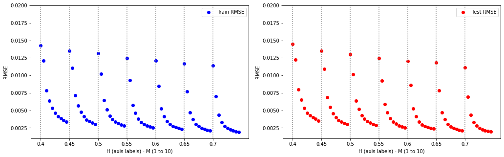
Figure 1: Factorial error (RMSE) decay as a function of H

For readibility, the detailed numerical results figures are included in Appendix Drawdown market generator, where Figures 6 to 8 investigate the root-mean-squared ($RMSE$) approximation error of the approximation for these individual dimensions. Figure 1 is included in the main text, as it gives a good overview of the expected rate decay as a function of $H$ and $M$ and the consistency for large sample sizes $K$.

We are initially interested in the consistency of the regressions and evaluate the in- and out-of-sample discrepancy as a function of sample size. Figure 6 shows the difference between in- and out-of-sample accuracy as a function of sample size $log(K)$. We averaged the difference for all simulation sizes over the values of $M$ to get a line per value of $H$ (blue line), the opposite (red line) or the overall average per $K$ (black line).

The conclusions are twofold: (1) when $K$ grows large the discrepancy disappears, which relates to Proposition 4.1 in the sense that for $K\rightarrow\infty$ the two error components (terms A and C) that explain differences in in- and out-of-sample performance shrink to zero, and (2) the in-sample(IS)/out-of-sample(OOS) accuracy divergence depends on confounders $M$ and $H$ implying an improperly chosen $M$ for smaller and/or rougher samples might lead to bad generalization (term B in error decomposition).

Next, we look in Figure 7 at the train and test $RMSE$ as a function of the signature approximation order $M$. When taking the average performance over $K$ and $H$, we find uniform decay in $RMSE$. When deconfounding for sample size $K$, which you can find on the right hand side of Figure 7, we find that only for the smallest sample size the improvement in test accuracy stalls before $M$ reaches its maximum value. This implies that for large samples sizes one would prefer to choose the highest signature order that is possible given computational constraints, i.e. the computing time scales quadratically with the signature order $M$ while the improvement in accuracy has diminishing returns (also see Figure 2). In sum, this indicates worse generalization abilities for smaller samples driven by the distances discussed in Proposition 4.1, rather than the $M/K$ ratio as it is small for all experiments.

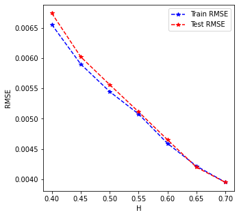
Figure 8: Train and test $RMSE$ as a function of the roughness $H$

Next, we check the relationship between the accuracy of the approximation and the roughness $H$ of the assumed process. In Figure 8, which shows the average $RMSE$ per level of $H$, we find that the accuracies improve uniformly with $H$.

Finally, the factorial error decay in $M$ and the dependency of its rate on $H$ is best illustrated in Figure 1. The vertical lines separate the different levels of $H$, denoted on the x-axis, while in between $M$ increases from 1 to 10, while $K$ is fixed at the maximum $50000$. It is clear that for rougher processes the error is higher and decreases slower than for smoother processes, which we derived from Eq. (8). For all levels of $H$, high orders of $M$ yield negligible approximation errors for this high $K$. Moreover, the in-sample decay generalizes well to out-of-sample error behaviour.

In summary, the simulation study confirms our initial expectations of rate decay and IS-OOS consistency, but raises some practical warnings as well:

• For a large number $K$ of sample paths, say $log(K)>3$, one finds uniform decay in $\kappa$ with both $H$ and $M$, in both test and training fits. In terms of Proposition 4.1, the distances between any $S$ and the $S_{k}$ do become smaller with $K$ and the estimated $\hat{L}$ generalize better.

• For small samples ($log(K)<3$), the unbiased approximation may generalize badly, which will result in worse accuracies for $ElNetCV$. This relates to Proposition 4.1 in the sense that the distance between any $S$ and $S_{k}$ (in inf-norm and signature terms) can be large. In any case, $M$ needs to be chosen high enough for rough paths, but with small $K$ the system might become ill-conditioned or even degenerate. High regularization will then result from CV, which comes at the cost of higher bias and lower (even IS) accuracy. This issue is very dependent on the sample and its roughness, but we generally discourage the approximation for sample sizes $log(K)<3$.

6.1.2 Empirical data

Data description and set up

Consider a universe of $U{=}4$ investible instruments: equity (S&P500), fixed income (US Treasuries), commodities (GSCI index) and real estate (FTSE NAREIT index). We collect price data (adjusted close prices) between Jan 1989 and May 2022, which gives us T=8449 daily observations. Clearly, these 4 different asset classes have different return, volatility and drawdown characteristics, which argues for combination and diversification. This can clearly be seen from Figure 9.

As an investor, we hold a portfolio $\mathbf{w}$, $w_{i},i\in{1,...,U}$, which allocates a weight $w_{i}$ to each investible asset. In these experiments, we attach $P\in\mathbb{N}$ sets of weights to these assets and pick a $\tau<T$ such that we have $T-\tau$ overlapping sample paths or a simple buy-and-hold strategy over $\tau$ days for every $p\in[0,...,P]$. Here we pick $\tau=20$, so we model monthly sample paths of these mixed asset class portfolios.

The drawdown distribution of the sample paths of such a hypothetical portfolio is shown in Figure 10. If the investor finds scenarios that breach certain levels of drawdowns over the course of a particular month, she needs to reallocate and increase her weights in lower-drawdown instruments. For instance, through drawdown optimization [10]), rescaling all portfolio weights with a risk-free cash-like fraction $w_{i}(1-w_{cash})$ that exhibits no drawdowns (CPPI [40] or TIPP [41] strategy), or by buying drawdown insurance instruments such as a barrier option [7][8]. However, traditional (G)BM-implied distributions understate these probabilities. In Figure 10, we compare the distribution with the distribution that is implied by standard simulated Brownian motion with the same volatility $\sigma$ parameter as the portfolios we have constructed. Note that one could also use the closed forms from Douady et al. [21], Rej et al. [20] and alike here. Importantly, we notice that the blue density is merely an optimistic lower bound on the true distribution of portfolio drawdown, and misses out on the tails. This can also be seen in Figure 11. The direct analytical link between generalized stochastic processes and this distribution is far from trivial, as one can not rely on Lévy’s theorem anymore (in contrast to the theoretical (G)BM case). In the next section, our methodology thus advocates a non-parametric approach to simulate paths that closely resemble the correct drawdown distribution. We will adapt parameterized paths $S_{\theta}$ such that their drawdown distribution converges towards this empirical drawdown distribution.

In this simulation we will:

• Generate a set of portfolio weights $\mathbf{w}_{p}$ (index $p$ for portfolio) and construct $T-\tau$ paths, based on taking blocks $b$ from the product of $w_{p}$ and $S$’s cumulative returns, the univariate portfolio paths $S_{p}$.

• Calculate the drawdown $\Xi(S_{p}^{b})$ and signatures $\Phi^{M}(S_{p}^{b})$ for each block and regress the two (for increasing $M$ in [1, …, 10]), with defining the $(1-p_{test})(T-\tau)$ first blocks as train sample and remaining blocks as test sample. Note that there is a strict train-test separation in time.

• Repeat $P=100$ times and report average performance.

Results and discussion

Our conclusions are analogous to the bottom-up simulation experiments. The accuracies are shown in Table 1. We find consistent train and test $RMSE$ performance, which is expected given the large $K$. The average discrepancy in train-test RMSE is $0.00016041$, which is in line with Figure 6. In line with Figure 7, from $M>5$ we get accurate approximations of $\xi$, after which it further improves at a much slower rate.

The average and standard deviation of the computation time of one signature of a certain high order $M$ taken over $1000$ iterations are displayed in Figure 2. One finds diminishing improvements in $RMSE$ for exponential increase in compute time, which might be prohibitive for very large $K$. This will depend on the used hardware (the signatory package has built-in parallelization in its C++ backend) and own parallelization choices. For this sample the improvements in accuracy become negligible after $M>5$, so it is not worth it to include higher orders of $M$.

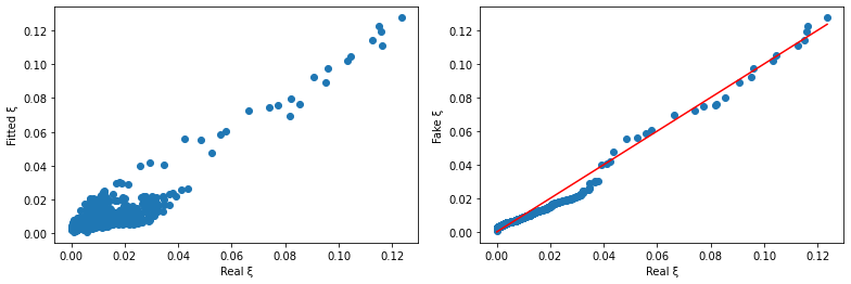
Figure 12: Train fit empirical data for one set of portfolio weights (equal weighted): scatter (left) and QQ plot (right)

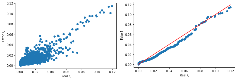
Figure 13: Test fit empirical data for one set of portfolio weights (equal weighted): scatter (left) and QQ plot (right)

This can also be seen from Figures 12 and 13 which show the train and test fit respectively for one set of portfolio weights (equal weighted). It becomes apparent that signatures linearize the relationship between portfolio paths and their drawdowns well and that this applies to both smaller and higher (tail) drawdowns. From these values we can deduce that improving accuracy in the order of a few basis points (bps) does not justify the exponential increase in compute. Moreover, from a market generator application perspective (next section) the replication of a drawdown up to a few bps in the objective function is likely to be spurious precision compared to total objective value.

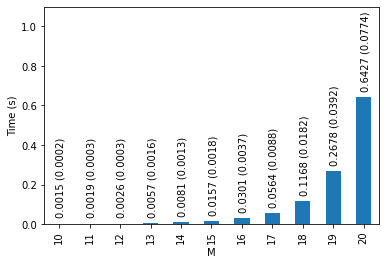
Figure 2: Average and standard deviation of compute times (in seconds) of a signature of order $M$ taken over 1000 iterations

M (K=8429, $P$ = 100)	RMSE Train		RMSE Test
1	0.010393	(0.002399)	0.013613	(0.003181)
2	0.009492	(0.002154)	0.012383	(0.002879)
3	0.008024	(0.001817)	0.009181	(0.002153)
4	0.007005	(0.001511)	0.006439	(0.001468)
5	0.006858	(0.001501)	0.006240	(0.001482)
6	0.006723	(0.001387)	0.006479	(0.003023)
7	0.006631	(0.001299)	0.006611	(0.003950)
8	0.006526	(0.001282)	0.006659	(0.006091)
9	0.006491	(0.001327)	0.006549	(0.006716)
10	0.006451	(0.001365)	0.006744	(0.004720)

Table 1: ElasticNet CV(10) fit for empirical data

6.2 Drawdown market generator: results and discussion

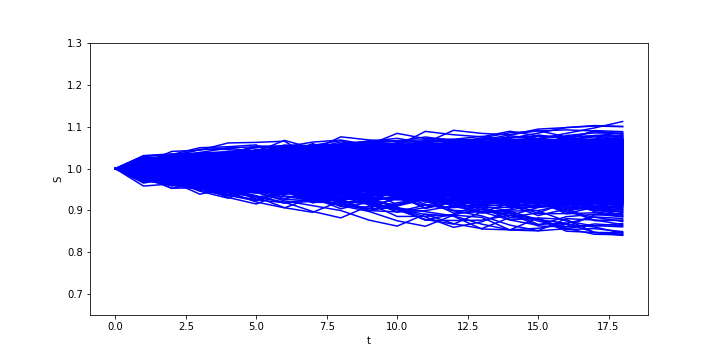
(a) Generated VAE

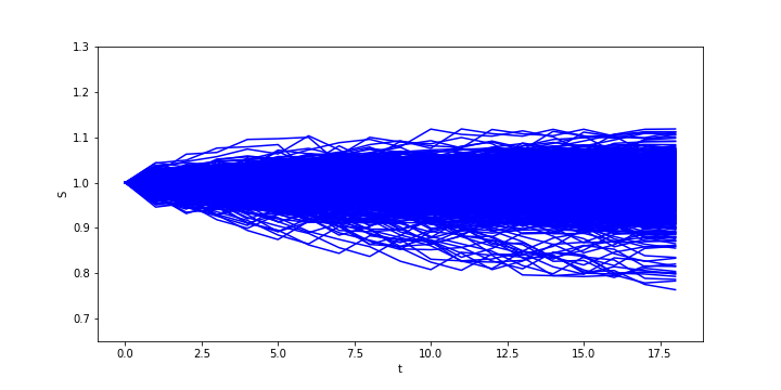
(b) Generated $\xi$-VAE

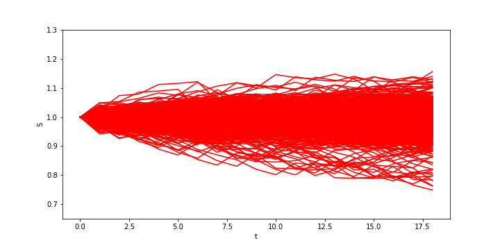
(c) Original

Figure 3: Generated paths versus original sample paths

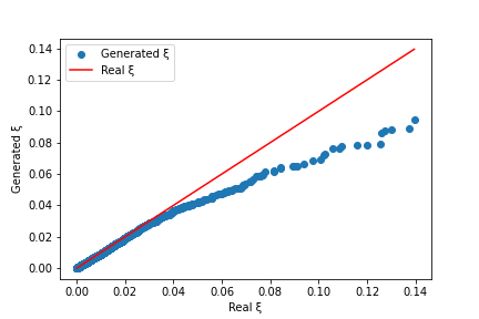
(a) VAE generated versus actual $\xi$ quantiles

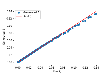
(b) $\xi$-VAE generated versus actual $\xi$ quantiles

Figure 4: Drawdown QQ plots

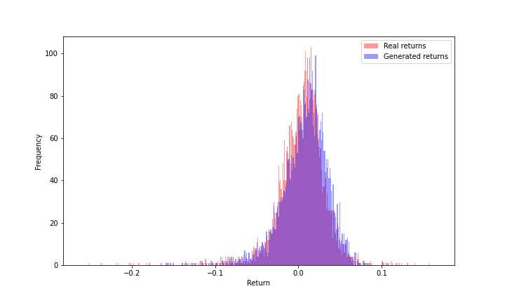
(a) Return distribution VAE

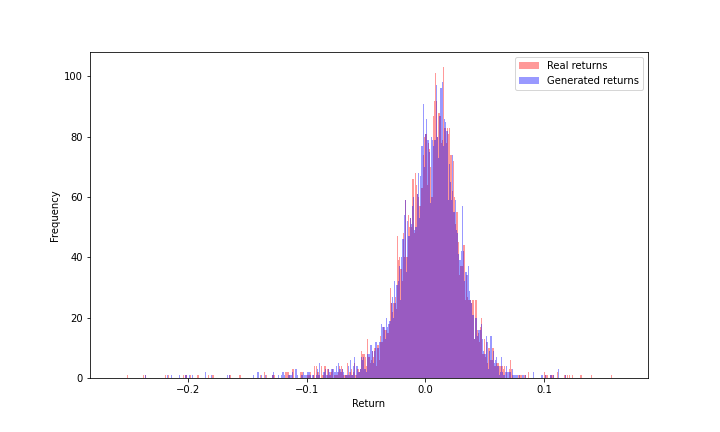
(b) Return distribution $\xi$-VAE

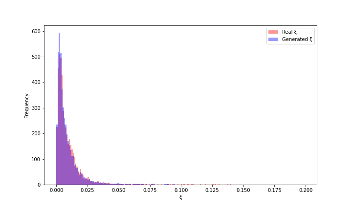
(c) Drawdown distribution VAE

(d) Drawdown distribution $\xi$-VAE

Figure 14: Generated versus actual drawdowns and returns distribution

The main findings are summarized in Figures 3 and 4. More details can again be found in the appendix on numerical results (Appendix 3: Numerical results). Figure 3 shows the generated paths of a standard VAE model versus the drawdown market generator, denoted by $\xi$-VAE. It is clear that the original VAE generates reasonably realistic scenarios, but is reminiscent of Figure 10 in the sense that the paths are non-Brownian but still too centered around the Brownian-like distribution (the densely colored areas). This is also clear from Figure 14. To summarize our architecture from this perspective, the standard VAE reconstruction term focuses on reproducing the top distribution ($L^{2}$ loss over a particular batch) such that it misses out on the tails. The $\xi$-VAE fits both the top and the bottom distribution such that it includes more tail (drawdown) scenarios. In sum, we find that the standard VAE shows a lack of more extreme adverse scenarios.

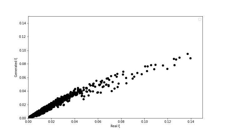
(a) VAE

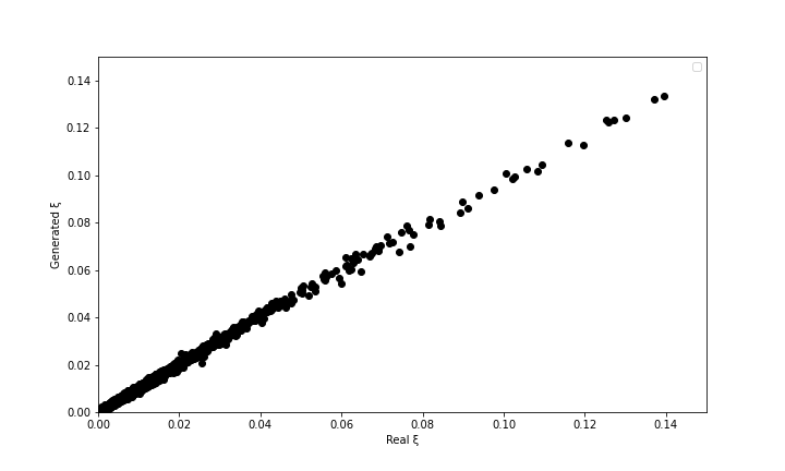
(b) $\xi$-VAE

Figure 15: Generated versus actual drawdowns scatter

This also becomes apparent in Figure 15, which plots the synthetic and actual drawdowns as a scatter. The standard VAE does a good job in capturing most part of the moderate drawdowns, but is scattered towards the higher drawdowns and produces none in the tail, while this is resolved with the $\xi$-VAE. Moreover, from the cumulative drawdown distribution the Kolmogorov-Smirnoff test that the synthetic drawdowns come from the same distribution as the original one cannot be rejected for both the standard and $\xi$-VAE, as we know the standard KS statistic is not sensitive to diverging tail distributions. A closely related graph is Figure 4, which plots the same scatter but using ordered observations (i.e. quantiles) and a first bisector line which would fit the data if the synthetic drawdown distribution has exactly the same quantiles as the original distribution. Again we find that the VAE misses out on capturing tail drawdown scenarios, while $\xi$-VAE does a much better job. This is not done by just memorizing the training samples and reproducing them exactly as the bottleneck VAE architecture forces a lower-dimensional representation of the training data (i.e. the non-parametric DGP). The autoencoder serves as a dimension reduction mechanism, rather than trivially mirroring the training data. That is why one sees different simulated paths than identical ones to the input samples, and why by using the trained decoder as a non-parametric DGP one can create an infinite amount of genuinely new data with the same distribution as the training data. Moreover, both train and validation losses flat out at convergence (please find Appendix Drawdown market generator loss convergence with details on the training and test convergence) while purely mirroring data would imply training losses would be minimal at the cost of high validation losses.

7 Conclusion

Learning functions on paths is a highly non-trivial task. Rough path theory offers tools to approximate functions on paths that have sufficient regularity by considering a controlled differential system and iterating the effect of intervals of the (rough) path on the (smooth) outcome function. One key path dependent risk functional in finance is a portfolio value path’s drawdown. This paper takes the perspective of portfolio drawdown as a non-linear dynamic system, a controlled differential equation, rather than directly analyzing the solution, or the exact expression of drawdown containing the running maximum operator. It relied on some important insights from the theory of rough paths to pinpoint that by taking this perspective, rather than continuous differentiability, a more general regularity condition of bounded changes in drawdown as a function of changes in input paths is sufficient to use a non-commutative exponential to interpolate between the two types of path dependent effects of a driving path on its resulting drawdown by numerically approximating the average nested effect. This thus allows one to locally approximate the drawdown function without having to evaluate its exact expression and in the meantime leapfrogging the inherent path dependence of its time derivatives. The linear dependence of a path’s drawdown on its differentiable signature representation then allows one to embed drawdown evaluations into systems of differentiable equations such as generative ML models. We prove this required regularity w.r.t. drawdown: the boundedness of its time derivatives allows us to write it in a more general controlled differential equation notation, and the Lipschitz regularity of the drawdown function assures bounded errors in its convergence proofs. That is why we then illustrated the consistency of the approximation: on simulated fractional Brownian and on real-world data, regression results exhibit a good fit for penalized linear regression (Elastic Net regression) when one has a reasonable sample size. Finally, our proposed application of the approximation is a so-called market generator model that evaluates the synthetic time series samples in terms of their drawdown. We argue that by including a drawdown learning objective, upon convergence of this reconstruction term in train and validation steps, one gets more realistic scenarios than the standard VAE model that exhibit quantifiably (i.e. the measured loss convergence) close drawdowns to the empirical ones, hence effectively reproducing the drawdown distributions without trivially mapping input paths to output paths.

Future work will focus on extending this application and further applying it to portfolio drawdown optimization, where one can for example test a data-hungry drawdown control strategy over a host of synthetic scenarios rather than the single historical one. In this context, learning drawdown scenarios can be seen as a denoising mechanism to first remove noise (encoding), then adding new noise (decoding new samples), then constructing an ensemble average strategy over a host of noisy scenarios that cancels out by construction instead of by assumption for historical scenarios (e.g. bootstrap methods). This non-parametric Monte Carlo idea could hence robustify one’s methodology further as a mathematically principled data augmentation technique. Moreover, the non-parametric nature of our Monte Carlo engine opens possibilities to full non-parametric pricing of path dependent (e.g. barrier) max drawdown insurance contingent claims.

Appendix: Controlled differential equations and path signatures

Controlled differential equations

We are generally interested in a CDE of the form:

$$dY_{t}=g(Y_{t})dX_{t}$$ (23)

where $X$ is a continuous path on $[0,T]\xrightarrow{}\mathbb{R}$, called the driving signal of the dynamic system. $g$ is a $\mathbb{R}\xrightarrow{}\mathbb{R}$ mapping called the physics that models the effect of $dX_{t}$ on the response $dY_{t}$. A controlled differential equation (CDE) distinguishes itself from an ordinary differential equation in the sense that the system is controlled or driven by a path ($dX$) rather than time ($dt$) or a random variable (stochastic SDEs, $d\varepsilon$).

Signatures

A series of coefficients of the path that naturally arrives from this type of equation is the series of iterated integrals of the path, or the path signature $\Phi$. The signature of a path $X:[0,T]\xrightarrow{}\mathbb{R}$ can be defined as the sequence of ordered coefficients:

$$\Phi(X)=(1,\Phi_{1},...,\Phi_{n},...)$$ (24)

where for every integer n (order of the signature):

$$\Phi_{n}(X)=\underset{u_{1}<...<u_{n},u_{1},...,u_{n}\in[0,T]}{\int...\int}dX_{u_{1}}\otimes...\otimes dX_{u_{n}}$$ (25)

where we define the $n$-fold iterated integral as all the integrals over the $n$ ordered intervals $u_{i}$ in [0,T]. The signature is the infinite collection for $n\xrightarrow{}\infty$, although typically lower level M truncations are used.

$$\Phi^{M}(X)=(1,\Phi_{1},...,\Phi_{M})$$ (26)

Picard Iterations

The idea behind a Picard iteration is to define for:

$$dY_{t}=g(Y_{t})dX_{t}$$ (27)

a sequence of mapping functions $Y(n):[0,T]\xrightarrow{}\mathbb{R}$ recursively such that for every $t\in[0,T]$:

$$Y(0)_{t}\equiv y_{0}$$ (28)

$$Y(1)_{t}=y_{0}+\int_{0}^{t}g(y_{0})dX_{s}$$ (29)

$$Y(n+1)_{t}=y_{0}+\int_{0}^{t}g(Y(n)_{s})dX_{s}$$ (30)

Now by simple recursion one finds that (for a linear $g$):

$$Y(n)_{t}=y_{0}+\sum_{k}^{n}g^{\otimes k}(y_{0})\underset{u_{1}<...<u_{n},u_{1},...,u_{n}\in[0,T]}{\int...\int}dX_{u_{1}}\otimes...\otimes dX_{u_{n}}$$ (31)

Such that a solution for $Y_{t}$ would be:

$$Y_{t}=y_{0}+\sum_{k}^{\infty}g^{\otimes k}(y_{0})\underset{u_{1}<...<u_{k},u_{1},...,u_{k}\in[0,T]}{\int...\int}dX_{u_{1}}\otimes...\otimes dX_{u_{k}}$$ (32)

This result shows how the signature, as an iterative representation of a path over ordered intervals, naturally arises from solving CDEs using Picard iterations, and how it is a natural generalization of Taylor series on the path space when the physics is linear.

$$g^{\circ 1}=g$$ (33)

$$g^{\circ n+1}=D(g^{\circ n})g$$ (34)

then it is natural to define the $N$-step Taylor expansion for $Y_{t}$ by $\hat{Y}(N)_{t}$ as:

$$\hat{Y}(N)_{t}=y_{0}+\sum_{n=1}^{N}g^{\circ n}(y_{0})\underset{u_{1}<...<u_{n},u_{1},...,u_{n}\in[0,T]}{\int...\int}dX_{u_{1}}\otimes...\otimes dX_{u_{n}}$$ (35)

Clearly, $\hat{Y}(N)_{t}$ is linear in the truncated signature of X up to order N.

Example

The simplest example of:

$$dY_{t}=g(Y_{t})dX_{t}$$ (36)

is a linear physics for a linear path X:

$$dY_{t}=Y_{t}dX_{t}$$ (37)

where:

$$g=g^{\circ 1}$$ (38)

$$g^{\circ n+1}=D(g^{\circ n})g$$ (39)

$$X_{t}=X_{0}+\frac{X_{T}-X_{0}}{T}t$$ (40)

and assuming:

$$y_{0}=1$$ (41)

$$X_{0}=0$$ (42)

Indeed, this yields the exponential function $Y_{t}=\exp(X_{t})$. For non-linear driving signals (where the order of the events matter), one generally gets a non-commutative version of the exponential function in Eq. (32)! For linear time, the order of events does not matter and we generally get the increment of the path raised to the level of the iterated integral, divided by the level factorial (i.e. the area of an $n$-dimensional simplex).

This can be seen from:

$$Y_{t}=y_{0}+\sum_{n=1}^{N}Y^{\circ n}\underset{u_{1}<...<u_{n},u_{1},...,u_{n}\in[0,T]}{\int...\int}dX_{u_{1}}\otimes...\otimes dX_{u_{n}}$$ (43)

now it is easy to see that:

$$\begin{split}\Phi^{n}=\underset{u_{1}<...<u_{n},u_{1},...,u_{n}\in[0,t]}{\int...\int}dX_{u_{1}}\otimes...\otimes dX_{u_{n}}\\ =\underset{0<u_{1}<...<u_{n}<t}{\int...\int}d(\frac{X_{t}}{t}u_{1})...d(\frac{X_{t}}{t}u_{n})\\ =\prod_{j=1}^{n}(\frac{X_{t}}{t})\underset{0<u_{1}<...<u_{n}<t}{\int...\int}du_{1}...du_{n}\\ =\frac{1}{t^{N}}\prod_{j=1}^{n}(X_{t})\frac{t^{N}}{n!}=\frac{(X_{t})^{n}}{n!}\end{split}$$ (44)

such that:

$$Y_{t}=y_{0}+\sum_{n=1}^{N}y_{0}\frac{1}{n!}(X_{t})^{n}=1+(X_{t})+\frac{(X_{t})^{2}}{2!}+\frac{(X_{t})^{3}}{3!}+...$$ (45)

Which is the classical Taylor expansion for the exponential function, i.e. linear physics integrated over a linear path (time). Now the signature approximation is the generalization of this idea to the path space (i.e. Y is a function on a path), where the path $X_{t}$ need not be a linear map of time, and the physics $g$ need not be linear (e.g. drawdown Eq. (5)).

Appendix 2: Variational Autoencoders

This section gives an overview of the variational autoencoder architecture. VAEs converge fast, are more stable than competing architectures, and they allow us to interpret the (conditional) distributions after training.

Below, we discuss the mappings $f_{\Theta}(X)$ and $f^{-1}_{\Theta}(Z)$ between the data and latent distributions, the original loss function $\mathcal{L}(X,X^{\prime})$ (which we revised in drawdown terms in this paper), the training algorithm and the hyperparameters.

General architecture

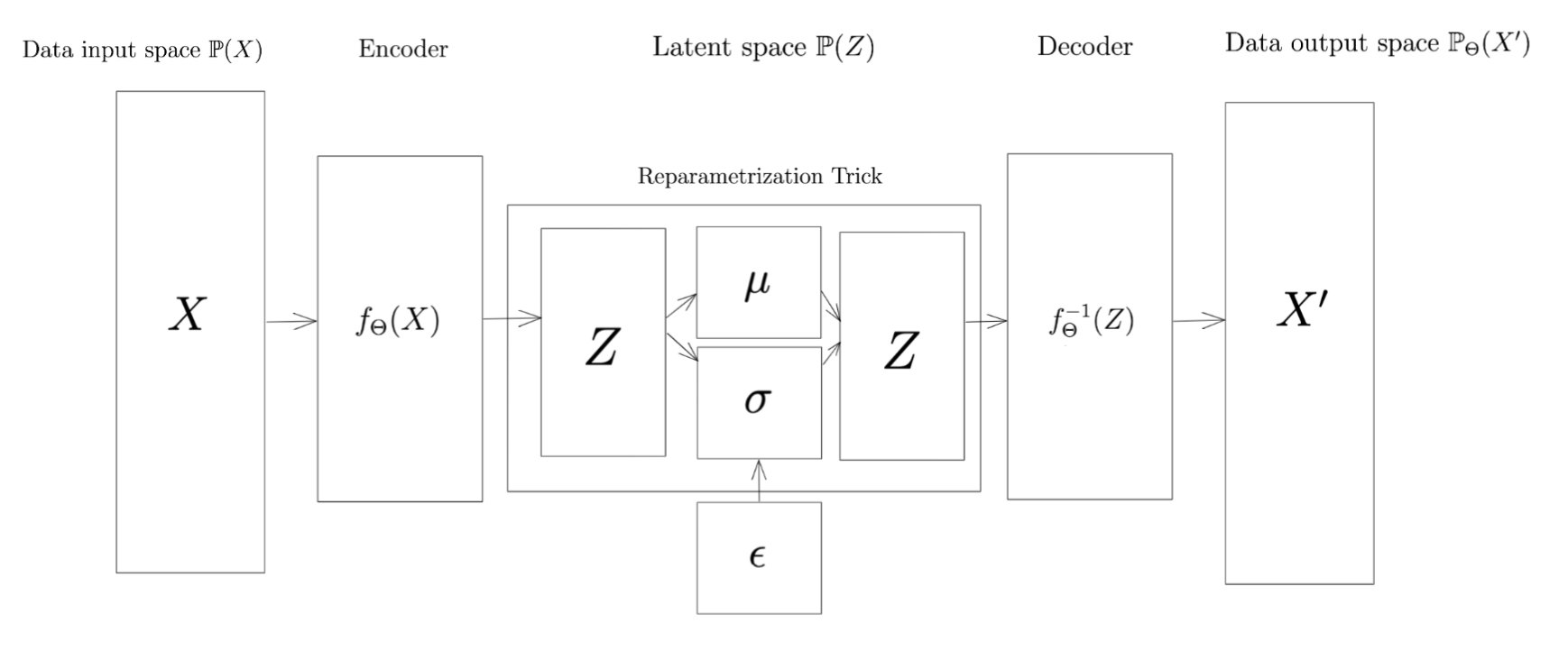
Figure 5: VAE architecture overview

The architecture of a VAE is summarized in Figure 5. As input we have a $D_{p}$-dimensional space $X$, the physical data domain that we can measure. Using a flexible neural network mapping $f_{\Theta}:\mathbb{R}^{D_{p}}\rightarrow\mathbb{R}^{D_{l}},D_{l}<<D_{p}$, called the encoder, we compress the dimension of the data into a $D_{l}$-dimensional latent space $Z$, e.g. 10-dimensional. Using the reparametrization trick ([42]) we map $Z$ onto a mean $\mu$ and standard deviation $\sigma$ vector, i.e. onto a $D_{l}$-dimensional Gaussian, e.g. a 10-dimensional multi-variate normal distribution. Starting from multi-variate normal data, we can recombine $\mu$ and $\sigma$ into a $D_{l}$-dimensional $Z$. The decoder neural network $f^{-1}_{\Theta}:\mathbb{R}^{D_{l}}\rightarrow\mathbb{R}^{D_{p}}$ maps the latent space back to the output space $\mathbb{P}_{\Theta}(X^{\prime})$ where $X^{\prime}$ can be considered reconstructed samples in the training step, or genuinely new or synthetic samples in a generator step. The quality of the VAE clearly depends on the similarity between $\mathbb{P}(X)$ and $\mathbb{P}_{\Theta}(X^{\prime})$.

Encoder - decoder networks

Let us now zoom in on $f_{\Theta}(X)$ and $f^{-1}_{\Theta}(Z)$. Each neural network consist of one layer of $J$ mathematical units called neurons:

$$f_{\Theta_{j}}=A(\sum_{i}^{D_{l}}\theta_{i,j}x_{i})$$ (46)

Every neuron takes linear combinations $\theta_{i}$ of the input data point $x_{i}$ and is then activated using a non-linear activation function $A$, such as rectified linear units (ReLU), hyperbolic tangent (tanh) or sigmoid. In this paper we use a variant of ReLU called a leaky ReLU:

$$LReLU(x)=1_{x<0}\alpha x+1_{x\geq 0}x$$ (47)

where $\alpha$ is a small constant called the slope of the ReLU. The $J$ neurons are linearly combined into the next layer (in this case $Z$):

$$Z_{k}:=\sum_{j}^{J}\theta_{j,k}f_{\Theta_{j}}$$ (48)

for every $k$ in $D_{l}$. The decoder map can formally be written down like the encoder, but in reverse order.

Loss function

The loss function of a VAE generally consists of two components, the latent loss ($\mathcal{L}_{L}$) and the reconstruction loss ($\mathcal{L}_{R}$):

$$\mathcal{L}(X,X^{\prime})=\beta\mathcal{L}_{L}+(1-\beta)\mathcal{L}_{R}$$ (49)

The latent loss is the Kullback-Leibler discrepancy between the latent distribution under its encoded parametrization, the posterior $f_{\Theta}(X)=\mathbb{P}_{\Theta}(Z|X)$, and its theoretical distribution, e.g. multi-variate Gaussian $\mathbb{P}(Z)$. Appendix B in [38] offers a simple expression for $\mathcal{L}_{L}$. The reconstruction loss is the cost of reproducing $\mathbb{P}_{\Theta}(X^{\prime})$ after the dimension reduction step, and originally computed by the root of the mean squared error (RMSE or $L2$-loss) between X and X’.

$$\begin{split}\mathcal{L}(X,X^{\prime})=\beta\frac{1}{2}\sum_{k}^{K}(1+\sigma-\mu^{2}-\exp(\sigma))\\ +(1-\beta)\mathbb{E}(||X-X^{\prime}||^{2})\end{split}$$ (50)

Training

In terms of training, the learning algorithm is analoguous to most deep learning methods. Optimal loss values $\mathcal{L}^{*}$ are determined by stochastically sampling batches of data and alternating forward and backward passes through the VAE. For each batch the data is first passed through the encoder network and decoder network (forward pass), after which $\mathcal{L}$ is evaluated in terms of $\Theta$. At each layer, the derivative of $\mathcal{L}$ vis-a-vis $\Theta$ can easily be evaluated. Next (backward pass), we say the calculated loss backpropagates through the network, and $\Theta$ are adjusted in the direction of the gradient $\nabla_{\Theta}\mathcal{L}$ with the learning rate as step size. The exact optimizer algorithm we used for this is Adam (Adaptive moments estimation, [43]). Finally, we also use a concept called regularization, which penalizes neural models that become too complex or overparametrized. We used a tool called dropout, that during training randomly sets a proportion of parameters in $\Theta$ equal to zero, and leaves those connections at zero that contribute the least to the prediction.

Hyperparameters

In summary, the hyperparameters of this architecture are: (1) the number of neurons in the encoder, (2) the number of neurons in the decoder, (3) the latent dimension $D_{l}$, (4) the learning rate $l$, (5) the optimizer algorithm, (6) the dropout rate, (7) the batch size $N_{b}$, (8) batch length $\tau$ and (9) number of training steps $N_{t}$. We opted for the following set up, which was optimized using grid search: 50, 50, 10, 0.001, Adam, 0.01, 50, 20, 200 (with early stopping criteria).

Generation

After training, in the sampling or generation step, we start from a random $D_{l}$-dimensional noise $\epsilon\sim\mathbb{P}(Z)$ which is $D_{l}$-variate Gaussian. Now, we simply need one decode step to generate new samples of $\mathbb{P}_{\Theta}(X^{\prime})$.

Appendix 3: Numerical results

Consistency and convergence of linear drawdown approximation in the signature space

Figure 6: In- and out-of-sample accuracy difference as a function of sample size $log(K)$ (Red = averaging out over $H$ to get a line per value of $M$, blue = opposite and black is overall average over both M and H).

Figure 7: Train and test $RMSE$ (y-axis) as a function of signature approximation order $M$. Average over $K$ and $H$ is shown on the left. An average per $K$ is shown on the right.

Empirical data overview

Figure 9: Data overview: return, volatility and drawdown heterogeneity among asset classes.

Empirical drawdown distribution

Figure 10: Drawdown distribution of a real-world mixed asset class portfolio versus the fitted theoretical drawdown distribution if the underlying DGP would be Brownian Motion (BM) with the same average volatility as the sample paths.

Figure 11: Zoom on the tail of the empirical versus theoretical drawdown distribution.

Empirical data: drawdown approximation fit

Drawdown market generator

Drawdown market generator loss convergence

Figure 16: Drawdown market generator: total loss convergence (rescaled)

Figure 17: Drawdown market generator: latent (KL) loss convergence (rescaled)

Figure 18: Drawdown market generator: total reconstruction loss convergence (rescaled)

Figure 19: Drawdown market generator: drawdown reconstruction loss convergence (rescaled)

References

- Wiese et al. [2020] M. Wiese, R. Knobloch, R. Korn, P. Kretschmer, Quant gans: Deep generation of financial time series, Quantitative Finance 20 (2020) 1419–1440.
- Koshiyama et al. [2021] A. Koshiyama, N. Firoozye, P. Treleaven, Generative adversarial networks for financial trading strategies fine-tuning and combination, Quantitative Finance 21 (2021) 797–813.
- Cont et al. [2022] R. Cont, M. Cucuringu, R. Xu, C. Zhang, Tail-gan: Nonparametric scenario generation for tail risk estimation, arXiv preprint arXiv:2203.01664 (2022).
- Bergeron et al. [2022] M. Bergeron, N. Fung, J. Hull, Z. Poulos, A. Veneris, Variational autoencoders: A hands-off approach to volatility, The Journal of Financial Data Science 4 (2022) 125–138.
- Buehler et al. [2020] H. Buehler, B. Horvath, T. Lyons, I. P. Arribas, B. Wood, A data-driven market simulator for small data environments, arXiv preprint arXiv:2006.14498 (2020).
- Vuletić et al. [2023] M. Vuletić, F. Prenzel, M. Cucuringu, Fin-gan: Forecasting and classifying financial time series via generative adversarial networks (2023).
- Carr et al. [2011] P. Carr, H. Zhang, O. Hadjiliadis, Maximum drawdown insurance, International Journal of Theoretical and Applied Finance 14 (2011) 1195–1230.
- Atteson and Carr [2022] K. Atteson, P. Carr, Carr memorial: Maximum drawdown derivatives to a hitting time, The Journal of Derivatives 30 (2022) 16–31.
- Chekhlov et al. [2004] A. Chekhlov, S. Uryasev, M. Zabarankin, Portfolio optimization with drawdown constraints, in: Supply chain and finance, World Scientific, 2004, pp. 209–228.
- Chekhlov et al. [2005] A. Chekhlov, S. Uryasev, M. Zabarankin, Drawdown measure in portfolio optimization, International Journal of Theoretical and Applied Finance 8 (2005) 13–58.