Navigating Out-of-Distribution Electricity Load Forecasting during COVID-19: Benchmarking energy load forecasting models without and with continual learning

Abstract.

In traditional deep learning algorithms, one of the key assumptions is that the data distribution remains constant during both training and deployment. However, this assumption becomes problematic when faced with Out-of-Distribution periods, such as the COVID-19 lockdowns, where the data distribution significantly deviates from what the model has seen during training. This paper employs a two-fold strategy: utilizing continual learning techniques to update models with new data and harnessing human mobility data collected from privacy-preserving pedestrian counters located outside buildings. In contrast to online learning, which suffers from ’catastrophic forgetting’ as newly acquired knowledge often erases prior information, continual learning offers a holistic approach by preserving past insights while integrating new data. This research applies FSNet, a powerful continual learning algorithm, to real-world data from 13 building complexes in Melbourne, Australia, a city which had the second longest total lockdown duration globally during the pandemic. Results underscore the crucial role of continual learning in accurate energy forecasting, particularly during Out-of-Distribution periods. Secondary data such as mobility and temperature provided ancillary support to the primary forecasting model. More importantly, while traditional methods struggled to adapt during lockdowns, models featuring at least online learning demonstrated resilience, with lockdown periods posing fewer challenges once armed with adaptive learning techniques. This study contributes valuable methodologies and insights to the ongoing effort to improve energy load forecasting during future Out-of-Distribution periods.

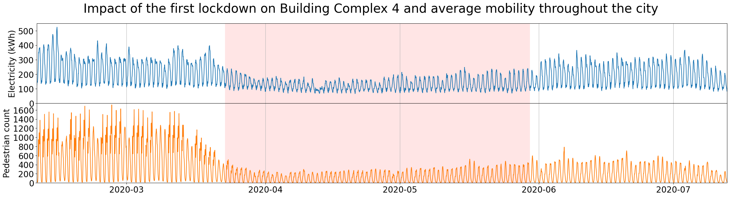
Figure 1. This figure illustrates the impact of the first COVID-19 lockdown (indicated by the red region) on the electricity load of a building complex located in Melbourne’s Central Business District (top graph). Concurrently, it presents the effect on the average human mobility throughout the city, as measured by pedestrian count (bottom graph). The diagram clearly shows significant shifts in distributions during the lockdown, which do not fully revert to their pre-lockdown state even after restrictions are lifted.

1. Introduction

Buildings play a significant role in energy consumption, making accurate electricity load forecasting essential for effective energy management and maintaining a balance in power grids. However, accurate forecasting is a challenging task since the building energy usage is primarily influenced by behaviours or activities of the occupants that are highly dynamic and heterogeneous (Chen et al., 2021). This can be exacerbated during Out-of-Distribution periods, such as the COVID-19 pandemic and lockdowns, presenting unique challenges due to changes in occupancy patterns and energy usage behavior. During these anomalous periods, we show that traditional machine learning and deep learning methods struggle to adapt, highlighting the need for different approaches that can effectively capture and account for shifting dynamics.

1.1. Online and Continual Learning

In conventional timeseries forecasting using machine learning, models are trained on a fixed training dataset and stop learning once deployed. Consequently, these models cannot adapt to changes in underlying data patterns during deployment. Online Learning (OL) has emerged as a promising solution to this challenge, as it enables building managers to adapt to changes in occupancy patterns and adjust energy usage accordingly. With OL, models can be updated incrementally with each new data point, allowing them to learn and adapt in real-time (Hoi et al., 2021). Furthermore, a subset of OL method called continual learning offers an even more powerful solution by addressing the issue of catastrophic forgetting (Lin, 1992; Chaudhry et al., 2019). These methods allow models to retain previously learned information while accommodating new data, preventing the loss of valuable insights and improving generalization in out-of-distribution scenarios. With continual learning technique, energy forecasting models can achieve robustness, adaptability, and accuracy, making them well-suited for handling the challenges posed by spatiotemporal data with evolving distributions.

1.2. Human Mobility as a Proxy to Occupancy Behaviour

Moreover, accurately forecasting buildings electricity load is challenging due to the dynamic and diverse nature of occupant behaviors, which are often not directly observable. Occupancy data is crucial (Hosseini et al., 2022; Anand et al., 2021) but difficult to obtain due to privacy concerns, the absence of occupancy sensors in legacy buildings, high sensor installation costs, and issues related to sensor accuracy. Researchers have explored various proxy information sources for occupancy sensing, such as Google search trends (Fu and Miller, 2022), positional records from Twitter (Mohammadi and Taylor, 2017), Call Details Recore (Bogomolov et al., 2016), Wi-Fi-derived occupancy (Nweye and Nagy, 2020), Bluetooth low energy on mobile devices (Tekler et al., 2020), domestic water consumption (Fu et al., 2021), and indoor carbon dioxide measurements (Wei et al., 2022). However, there has been limited focus on leveraging human mobility-related spatial-temporal data for energy use modeling (Miller et al., 2022). While occupancy sensors provide complete observation of people in buildings, pedestrian sensors only capture partial pedestrian flows, making the utilization of traffic data for energy modeling more challenging. In this study, we investigate the extent to which we can leverage pedestrian sensors data to improve electricity load forecasting.

1.3. Contributions

In this study, we evaluate the effectiveness of mobility data and continual learning for forecasting buildings electricity load during out-of-distribution periods. We utilized real-world data from Melbourne, Australia, a city that experienced one of the strictest lockdowns globally (Boaz, 2021), making it an ideal case study. We conducted experiments using data from 13 building complexes to empirically assess the performance of these methods. Our contributions are as follows:

1. Our dataset provides a high spatial granularity, covering 13 buildings in Melbourne, Australia, which experienced one of the longest and strictest lockdowns globally.

2. We demonstrate the superiority of continual learning over traditional OL and non-OL methods, particularly during out-of-distribution periods. Classical machine learning and deep learning methods experience poor performance during out of distribution scenarios.

3. Incorporating mobility data as a feature holds potential for enhancing forecasting accuracy, but its applicability should be carefully evaluated to prevent overfitting.

4. Our study reveals that forecasting during lockdown periods was surprisingly easier than pre-lockdown periods, but this observation is valid only when employing online or continual learning approaches.

2. Related Works

2.1. Energy Prediction in Urban Environments

Electricity demand profiling and forecasting has been a task of importance for many decades. Nevertheless, there exist a limited number of work in literature that investigate how human mobility patterns are directly related to the urban scale energy consumption, both during normal periods as well as adverse/extreme events. Energy modelling in literature is done at different granularities, occupant-level (personal energy footprinting), building-level and city-level. Models used for energy consumption prediction in urban environments are known as Urban Building Energy Models (UBEM). While top-down UBEMs are used for predicting aggregated energy consumption in urban areas using macro-economic variables and other aggregated statistical data, bottom-up UBEMs are more suited for building-level modelling of energy by clustering buildings into groups of similar characteristics (Ali et al., 2021). Some examples in this respect are SUNtool, CitySim, UMI, CityBES, TEASER and HUES. Software modelling (simulation-based) is also a heavily used approach for building-wise energy prediction (Eg: EnergyPlus (Crawley et al., 2001)). Due to fine-grain end-user level modelling, bottom-up UBEMs can incorporate inputs of occupant schedules. There also exist occupant-wise personal energy footprinting systems. However, for such occupant-wise energy footprinting, it requires infrastructure related to monitoring systems and sensors for indoor occupant behaviours, which are not always available. Also, due to privacy issues, to perform modelling at end-user level granularity, it can be hard to get access to publicly available data at finer temporal resolutions (both occupancy and energy) (Wei and Jiang, 2019). Building-wise energy models also have the same problems. Simulation-based models have complexity issues when scaling to the city level, because they have to build one model per each building. Moreover, simulation-based models contain assumptions about the data which make their outputs less accurate (Ali et al., 2020). Consequently, it remains mostly an open research area how to conduct energy forecasting with data distribution shifts.

2.2. Mobility Data as Auxiliary Information in Forecasting

The study of human mobility patterns involves analysing the behaviours and movements of occupants in a particular area in a spatio-temporal context (Salim et al., 2020). The amount of information that mobility data encompasses can be huge. The behaviour patterns of humans drive the decision making in many use-cases. Mobility data in particular, can act as a proxy for the dynamic (time varying) human occupancy at various spatial densities (building-wise, city-wise etc.). Thus such data are leveraged extensively for many tasks in urban environments including predicting water demand (Smolak et al., 2020), urban flow forecasting (Xue and Salim, 2021; Xue et al., 2021), predicting patterns in hospital patient rooms (Dedesko et al., 2015), electricity use (Hewamalage et al., 2023) etc. that depend on human activities.

Especially, during the COVID19 pandemic, mobility data has been quite useful for disease propagation modelling. For example, in the work by (Wang et al., 2020), those authors have developed a Graph Neural Network (GNN) based deep learning architecture to forecast the daily new COVID19 cases state-wise in United States. The GNN is developed such that each node represents one region and each edge represents the interaction between the two regions in terms of mobility flow. The daily new case counts, death counts and intra-region mobility flow is used as the features of each node whereas the inter-region mobility flow and flow of active cases is used as the edge features. Comparisons against other classical models which do not use mobility data has demonstrated the competitiveness of the developed model.

Nevertheless, as (Salim et al., 2020) state, the existing studies involving human mobility data lack diversity in the datasets in terms of their social demographics, building types, locations etc. Due to the heterogeneity, sparsity and difficulty in obtaining diverse mobility data, it remains a significant research challenge to incorporate them in modelling techniques (Ali et al., 2021). Yet, the lack of extracting valuable information from such real-world data sources remains untapped, with a huge potential of building smarter automated decision making systems for urban planning (Salim et al., 2020).

2.3. Deep Online and Continual Learning

Deep learning methods have been used for many mobility data and tasks, such as flight delay prediction (Shao et al., 2022), map inference (Prabowo et al., 2019) and time-series forecasting (Prabowo et al., 2023b, c, d; Liu et al., 2023). Moreover, methods such as Long Short-Term Memory (LSTM) (Pełka and Dudek, 2020), Neural basis expansion analysis for interpretable time series forecasting (N-BEATS) (Oreshkin et al., 2021) and transformers (Xue and Salim, 2023) have been widely used for electricity load forecasting. However, a common challenge for deep learning methods is the performance degradation during out-of-distribution periods. Online learning methods have been proposed to address this, but they can suffer from catastrophic forgetting (Salim et al., 2020). To mitigate this, continual learning methods such as Fast and Slow Network (FSNet) (Pham et al., 2022) have been developed. These methods aim to retain past knowledge while adapting to new data, improving generalization in OOD scenarios.

3. Datasets

In this section, we will discuss the sources and composition of the datasets used in our research. This includes the electricity load dataset, the division of our timeline into five distinctive periods aligning with the lockdowns due to COVID-19, the human mobility data captured by automated pedestrian counting systems, and the temperature data.

Table 1. The summary statistics of the energy dataset from 13 anonymized building complexes (BCs).

BC	start	end	duration (years)	mean (kWh)	std. (kWh)	min (kWh)	0.25 (kWh)	median (kWh)	0.75 (kWh)	max (kWh)
1	2018-08-01	2020-12-31	2.42	276.73	99.68	19.38	213.31	280.78	347.45	686.01
2	2019-02-13	2020-12-31	1.88	12.33	6.68	0.00	8.50	10.31	13.65	50.16
3	2019-01-01	2020-12-31	2.00	207.27	111.59	3.25	112.72	169.29	297.33	611.67
4	2019-01-01	2020-12-31	2.00	223.27	108.37	0.00	134.52	199.20	307.09	611.18
5	2019-01-01	2020-12-31	2.00	12.94	9.65	3.68	5.77	8.85	17.65	55.26
6	2018-01-01	2020-12-31	3.00	278.17	88.67	1.32	203.38	272.68	342.10	709.41
7	2018-01-01	2020-12-31	3.00	166.42	66.60	5.38	112.62	144.34	206.63	371.64
8	2018-01-01	2020-12-31	3.00	160.09	96.24	11.25	92.68	120.79	217.45	550.47
9	2019-01-01	2020-12-31	2.00	72.83	33.64	1.80	45.18	66.71	96.57	218.07
10	2019-01-01	2020-12-31	2.00	34.48	29.20	5.51	14.80	21.76	41.00	123.90
11	2019-07-01	2020-12-31	1.50	26.64	13.21	0.00	17.45	21.75	31.06	83.01
12	2019-01-01	2020-12-31	2.00	0.90	1.04	0.20	0.28	0.62	0.96	15.08
13	2018-01-01	2020-10-31	2.83	293.53	96.17	0.23	231.14	286.68	351.01	675.15

3.1. Electricity Load

This research relies on electricity data obtained from electricity suppliers, with privacy being a paramount consideration. To protect the privacy of building owners, operators, and users, nearby buildings are aggregated into anonymized Building Complexes (BCs). These BCs consist of mixed-use properties, encompassing residential, office, and retail spaces. The dataset under analysis is derived from thirteen such BCs located around Melbourne’s Central Business District, Australia. four of these BC datasets have been previously published (Prabowo et al., 2023a).

A statistical summary of the data is provided in Table 1 and its visual representation can be found in Figure 1. The dataset maintains an hourly granularity, presenting a detailed view of energy consumption. It is noteworthy that this dataset displays considerable variation in scale, with the mean value of BC 13 being about 300 times that of BC 12.

3.2. Lockdown Time Periods

The Melbourne lockdown timelines are complex due to the varying levels of restrictions imposed at different stages. Consequently, it’s not a simple binary state of lockdown versus no lockdown. Despite these complexities, for the purpose of our study, we’ve categorized the timeline into five distinct periods:

• Pre-Lockdown: The period before the first lockdown.

• First lockdown starts on 23rd March 2020 (Library et al., 2021).

• First Lockdown.

• First lockdown ends on 30th May 2020.

• Inter-Lockdown One: The period between the end of the first lockdown and the start of the second lockdown.

• Second lockdown starts on 2nd August 2020 (Andrew, 2020a).

• Second Lockdown.

• Second lockdown ends on 27th October 2020 (Andrew, 2020b).

• Inter-Lockdown Two: The period from the end of the second lockdown until the end of 2021, which concludes our datasets.

3.3. Human Mobility Data

Mobility data was obtained from an automated pedestrian counting system deployed by the City of Melbourne, which tracked pedestrian movements throughout the city without collecting any personal information, as no video was recorded. From the 79 installed sensors, we chose 42 that provided complete coverage over our desired timeframe, taking into account the varying installation times, as well as instances of relocation and removal. A detailed description of this data is not provided herein as they are publicly accessible (of Melbourne, [n. d.]).

3.4. Temperature

We sourced temperature records from the National Renewable Energy Laboratory (NREL) (Sengupta et al., 2018) Asia Pacific Himawari Solar Data. Given the close proximity of the BCs, the same temperature data was utilized for all.

4. Experiments

4.1. Problem Definition

We define the forecasting problem as follows. Given the recent past observation $\mathbf{X}\in\mathbb{R}^{W\times|F|}$ where $W\in\mathbb{Z}^{+}$ is the length of the observation window and $F$ is the feature set (descibed later), the task to forecast the electricity load in the near future $\mathbf{Y}\in\mathbb{R}^{H}$ where $H$ is the forecasting horizon. Thus, $f(\mathbf{X})=\mathbf{Y}$.

4.2. Online Learning Setup

Our experimental setup is designed to evaluate the model’s ability to generalize during Out-of-Distribution periods. We adopt a time-based splitting strategy to divide the dataset. The model’s initial training is performed on the first three months of the data, referred to as the ’warm-up’ period.

After this initial setup, we incorporate two separate strategies for the rest of the data: Classical: In this approach, no further training is done post the warm-up period. The model, once trained, is used as is to forecast for the remaining period. Online Learning (OL): In this method, the model undergoes a gradient descent step for every new incoming data point i.e. $\mathtt{batch\_size}=1$. It implies that the model learns and updates sequentially from each new data point.

For hyperparameter tuning, the validation set consists of one month of data following the three months used for training / warm-up.

4.3. Feature Sets

We explore the role of human mobility in comparison with temperature in forecasting by testing four different feature sets ($F$). This is done to understand how these variables contribute to the model’s performance.

• $|F_{1}|=3=1\ E+1\ HoD+1\ DoW$ where $E$ is Energy Use, $HoD$ is the hour-of-day, and $DoW$ is the day-of-week.

• $|F_{2}|=47=|F_{1}|+42\ M+1\ \bar{M}_{micro}+1\ \bar{M}_{macro}$ where each $M$ is pedestrian counter, $\bar{M}_{micro}$ is the micro-average of the pedestrian counter, and $\bar{M}_{micro}$ is the macro-average of the pedestrian counter. Micro-average is the usual average, while in macro-average, each pedestrian counter timeseries is [0,1] normalized first before averaging.

• $|F_{3}|=4=|F_{1}|+1\ T$ where $T$ is temperature.

• $|F_{4}|=48=|F_{2}|+1\ T$ uses all of the features.

4.4. Selected Methods

4.4.1. Naive

In this study, we employ 11 baseline methods, beginning with three naive approaches. In the CopyLastHour method, forecasts are simply generated by duplicating the last hour’s value, presuming smoothness in the time series. This is a common naive baseline in forecasting tasks (Prabowo et al., 2023c; Jiang et al., 2021). Similar in approach, CopyLastDay and CopyLastWeek are methods that replicate values from the previous day and week respectively, thus assuming periodic behaviors within the time series.

4.4.2. Statistical

Transitioning from the naive methods, we utilize Exponential Smoothing (ES). This method is a typical statistical non-learning method that, despite its simplicity, does involve a hyperparameter that we validate using the first month of data. Considering the rapid computational ability of ES, a thorough grid search is performed through all datasets for this hyperparameter, which is the smoothing factor ($\alpha$), ranging from $0<\alpha<1$ with a step size of $0.0001$. It is important to note that the first four methods are non-learning and univariate, and do not conform to the setup described earlier. We discovered that the best $\alpha$ is 1, thus ES is identical with CopyLastHour.

4.4.3. Machine Learning

Random Forest (RF) regression is a common machine learning algorithm (Breiman, 2001; Geurts et al., 2006). We use the implementation by www.scikit-learn.org version 1.2.2. The hyperparameter search space is uniformly distributed as follows:

• n_estimators, range=[1,200]

• max_depth, range=[1,50]

• min_samples_split, range=[0,1]

• min_samples_leaf, range=[0,1]

• min_weight_fraction_leaf, range=[0,0.5]

• max_features, range=[0,1]

• max_leaf_nodes, range=[2,50]

• oob_score, range=[0,1]

• max_samples, range=[0,1]

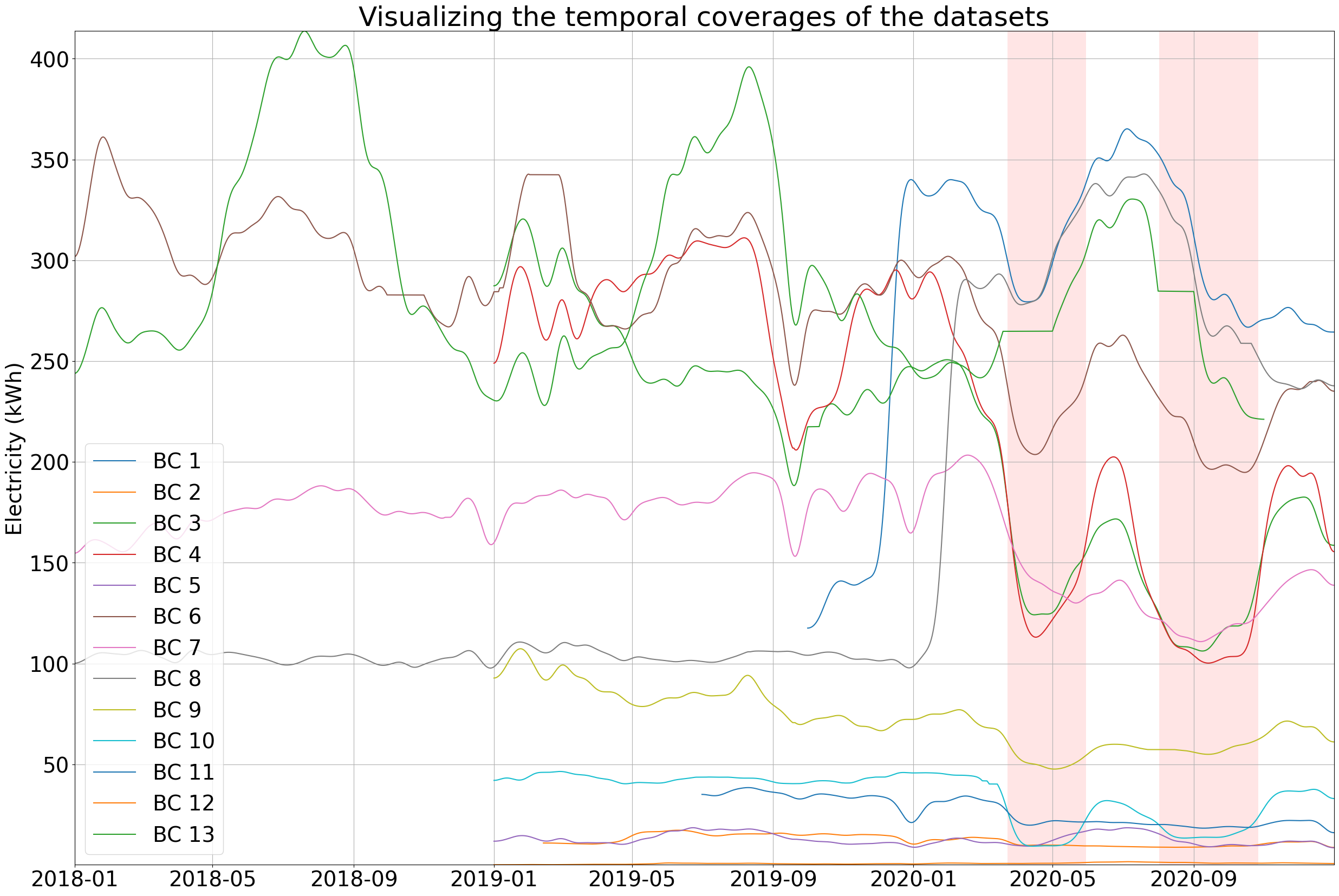
Figure 2. The visualization showcases electricity datasets from thirteen Building Complexes (BCs), emphasizing the inherent variations in electricity load across these BCs. It also highlights the significant changes in load patterns triggered by lockdowns. To facilitate the visualization, the plots smoothed using a Gaussian filter with a sigma of one week.

eXtreme Gradient Boosting (XGBoost) is another popular machine learning algorithm (Chen and Guestrin, 2016). It can handle many different task, and is also popular for timeseries forecasting (Herzen et al., 2022). We use the official implementation at xgboost.readthedocs.io/en/stable/python/python_intro.html version 1.7.5. The hyperparameter search space is as follows:

• max_depth, range = [1, 10], uniform distribution

• min_child_weight, range = [1e-4, 1e4], logarithmic distribution

• gamma, range = [1e-4, 1e4], logarithmic distribution

• subsample, range = [1e-8, 1.0], logarithmic distribution

• colsample_bytree, range = [1e-8, 1.0], logarithmic distribution

• eta.3, range = [1e-8, 1.0], logarithmic distribution

• alpha, range = [1e-8, 1.0, logarithmic distribution]

VAR is a common baseline for multi-variate timeseries (Prabowo et al., 2023b). We found differencing to be not helpful.

4.4.4. Deep Learning

A typical deep learning baseline for electricity load forecasting is Long Short-Term Memory (LSTM) (Pełka and Dudek, 2020; Oreshkin et al., 2021). We use our own PyTorch implementation. Following previous work (Oreshkin et al., 2021), we use a single LSTM layer, 20 epochs without early stopping, gradient clipping at L2 norm of 1. Because 3 months consist of about 2160 hourly timesteps, we pick a batch size of 64 and ended up with 33 weights updates per epoch. The hyperparameter search space is as follows:

• hidden_size, range = [50, 1000], uniform distribution.

• learning_rate, range = [1e-10, 1e-2], logarithmic distribution.

The generic version of Neural Basis Expansion Analysis for interpretable Time Series (NBEATS) have also been used for electricity load forecasting (Oreshkin et al., 2021). the original paper is univariate. While the original implementation is only for univariate forecasting, we adapt it to handle multivariate inputs by flattening the input data (Herzen et al., 2022). However, in feature set E, we do not include the time features as the original paper is designed for univariate forecasting. We use the official PyTorch implementation at www.github.com/ServiceNow/N-BEATS. The hyperparameter search space is as follows:

• stacks, range = [1, 10], uniform distribution.

• layers, range = [2, 4], uniform distribution.

• layer_size, range = [2, 4], uniform distribution.

• learning_rate, range = [1e-10, 1e-2], logarithmic distribution.

4.4.5. Online Learning

In the VAR+OL method, we apply OL to the VAR model using the Adam optimizer (Kingma and Ba, 2015). The learning rate is the only hyperparameter we tuned, and we set the range between $1\times 10^{-6}$ and $5\times 10^{-2}$.

Similarly, we also apply OL to LSTM and NBEATS to make LSTM+OL and NBEATS+OL, using the same hyperparameters as described in Section 4.4.4.

4.4.6. Continual Learning

Fast and Slow Network (FSNet) (Pham et al., 2022) is a deep continual learning method. We only search through the hyperparameters recommended in the original paper (Pham et al., 2022) as follows:

• $\gamma$ , range = (0, 1), uniform distribution.

• $\gamma^{\prime}$ , range = (0, 1), uniform distribution.

• $\tau$ , range = (0, 1), uniform distribution.

• learning_rate, range = [1e-10, 1e-2], logarithmic distribution.

4.5. Experimental Setups

In our experimental setup, we apply standard scaling to the data and utilize the Adam optimizer for all deep learning, online learning, and continual learning methods. We clamp or clip the model’s output between the minimum and maximum values in a time period (see Section 3.2). The mean absolute error (MAE) serves as the loss function. While various evaluation metrics are available, our focus primarily lies on showcasing the MAE metrics, as they provide consistent conclusions across different evaluation criteria. For models with hyperparameters, we employ Optuna (Akiba et al., 2019) with a budget of 20 runs to optimize their performance. Additionally, for stochastic models, we replicate the experiments 10 times with different random seeds and report the mean results.

4.5.1. Softward and Hardware

In our experiments, we utilized the following software: Python 3.9.2, PyTorch 1.9.0, Optuna 2.10.0, NumPy 1.20.0, and pandas 1.2.4. The experiments were conducted using the Google Colab PRO platform, with the release date set to June 2, 2023 and the Gadi high performance computing system www.top500.org/system/179865.

Table 2. The comprehensive results of all combinations of methods and feature sets for BC 8 are presented, utilizing the MAE as the error metric - where a lower value is indicative of better performance. The results are arranged in ascending order based on the PLD column, hence the top result in bold with lowest error is the best. FSNet is a popular model that incorporate continual learning.

Methods	Feat.	PLD	LD1	IL1	LD2	IL2
FSNet	EM	5.26	11.79	12.50	10.45	8.10
FSNet	ET	5.67	12.46	12.86	10.89	8.58
FSNet	E	5.76	13.59	14.44	11.81	9.09
NBEATS+OL	EM	7.01	16.41	17.90	17.41	13.79
FSNet	ETM	7.05	14.48	14.43	11.45	8.87
NBEATS+OL	E	7.90	15.74	18.05	16.47	13.75
NBEATS+OL	ETM	8.02	18.36	17.84	17.74	13.28
NBEATS+OL	ET	8.18	19.39	18.02	16.90	12.78
LSTM+OL	ETM	10.21	22.17	20.99	18.31	13.22
LSTM+OL	EM	10.75	21.66	22.05	17.35	13.45
LSTM+OL	E	11.41	21.36	22.47	17.60	13.48
NBEATS	EM	11.66	76.23	92.94	73.37	53.64
NBEATS	E	11.71	87.35	106.98	83.10	61.62
NBEATS	ET	12.30	84.76	110.95	77.96	59.28
LSTM+OL	ET	12.49	38.26	33.48	23.08	14.34
VAR	E	12.70	89.64	107.16	87.43	61.36
VAR+OL	E	12.70	89.64	107.16	87.43	61.36
VAR	ET	14.73	101.85	119.63	101.82	70.37
VAR+OL	ET	14.73	101.85	119.63	101.82	70.37
NBEATS	ETM	16.45	134.57	173.04	126.76	95.06
LSTM	ET	17.82	181.81	224.16	172.39	123.94
LSTM	E	18.01	180.27	220.82	171.09	125.25
LSTM	EM	18.05	185.04	227.54	175.75	127.55
LSTM	ETM	18.52	185.39	228.29	176.47	128.00
XGBoost	E	19.12	188.56	231.48	179.20	131.04
XGBoost	ET	19.16	189.34	232.74	180.14	130.90
RF	EM	19.49	191.75	234.62	182.22	134.48
XGBoost	ETM	21.36	192.14	235.06	182.23	134.75
RF	E	21.39	192.45	235.33	182.87	134.85
XGBoost	EM	21.81	191.20	234.22	180.25	134.80
RF	ET	25.25	193.53	236.40	183.95	135.93
RF	ETM	25.42	193.73	236.61	184.14	136.14
CopyLastWeek	E	45.26	57.21	38.31	32.90	53.17
CopyLastHour	E	53.66	50.62	60.68	40.08	65.93
ES	E	53.66	50.62	60.68	40.08	65.93
CopyLastDay	E	70.80	68.29	75.00	53.54	89.29
VAR	ETM	198.03	145.25	154.38	166.35	105.84
VAR+OL	ETM	198.03	145.25	154.38	166.35	105.84
VAR	EM	200.42	146.02	151.40	167.79	101.00
VAR+OL	EM	200.42	146.02	151.40	167.79	101.00

5. Results and Analysis

Due to space limitations, only a selection of results will be presented here, given the extensive number of experiments conducted, totaling $3380\textrm{ results}=$ $13\textrm{ BCs}\;\times\>$ $5\textrm{ periods}\;\times\>$ $4\textrm{ feature sets}\;\times\>$ $(4\textrm{ univariate}$ $\textrm{methods}\;+\>9\textrm{ multivariate methods})$. Instead, the complete results is publicly available here: https://github.com/aprbw/OoD_Electricity_Forecasting_during_COVID-19. Specifically, the full results will be displayed for BC 8, characterized by its extended duration and wide standard deviation, enabling the identification of notable patterns and trends within the dataset. Then, the analysis will be extended to other datasets to verify the generalizability of the findings and establish a more robust understanding of the implications of the research.

5.1. Building Complex 8

The results for all combinations of methods and feature sets for Building Complex 8 (BC 8) are displayed in Table 2. For stochastic methods, the mean of ten replications, each with a different random seed, is given.

For BC 8, the continual learning approach (FSNet) outperforms other methods, and incorporating the mobility feature proves beneficial. This trend holds true across all five periods. A horizontal line in the table separates the methods that outperform the naive baselines in at least one period from those that do not. All methods above this line employ OL or CL, highlighting their importance during Out-of-Distribution periods. Put differently, without the application of OL, these methods perform worse than the naive ones during Out-of-Distribution scenarios. Note that linear models like VAR struggle to effectively leverage mobility data.

FSNet significantly outperforms the second-best method (NBEATS + OL), showing an improvement ranging from 20% to 40%. The addition of mobility data (transitioning from FSNet ET to FSNet EM) leads to a smaller but still noticeable improvement, ranging from 3% to 10%. We will quantify the improvements brought by mobility data, when such is the case, for other datasets in Section 5.4. Interestingly, FSNet ETM performs worse compared to the other FSNet variants, suggesting that the inclusion of additional features increase the risk of overfitting.

Table 3. This table shows the best combinations of method and features for each BC. MAE is the error metric, lower is better.

BC	Methods	Feat.	PLD	LD1	IL1	LD2	IL2
1	VAR	E	8.04	8.76	11.18	9.83	7.92
2	FSNet	ET	2.37	1.20	1.04	0.80	1.57
3	FSNet	EM	15.63	10.33	9.59	7.15	12.32
4	FSNet	EM	16.04	9.48	11.06	6.99	11.80
5	FSNet	ETM	1.96	1.92	2.95	1.69	1.56
6	FSNet	E	14.71	11.19	11.32	9.50	9.85
7	FSNet	E	10.21	5.69	5.95	4.08	6.21
8	FSNet	EM	5.27	11.80	12.50	10.46	8.10
9	FSNet	E	4.68	2.31	3.56	1.93	4.31
10	FSNet	E	5.47	4.11	4.68	4.25	4.88
11	FSNet	ET	4.10	2.15	2.17	1.70	2.42
12	FSNet	ETM	0.22	0.26	0.47	0.27	0.20
13	FSNet	E	16.88	15.05	15.17	12.97	12.22

5.2. Best over all BCs

To assess the consistency of these trends across all BCs, we refer to Table 3, which only displays the best combinations of methods and feature sets for each BC for brevity. It is clear that FSNet is almost invariably the most effective method, thereby highlighting the crucial role of continual learning. Although not explicitly shown in the table, it is important to note that the most effective combinations of features and methods remain practically consistent across all five periods. This implies that FSNet remains the superior choice even during PLD.

While the benefits of adding extra features seem to vary, our findings indicate that mobility data provides an advantage in 5 out of 13 cases, and temperature data in 4 out of 13 instances. This suggests that, when feasible, it is always worthwhile to consider incorporating mobility data into the forecasting model as it may improve the forecast accuracy.

It is commonly assumed that out-of-distribution periods pose more significant challenges in forecasting. However, our analysis indicates a more nuanced picture. When comparing the forecasting accuracy across different time periods (horizontally on the table), we find that, for all BCs except 1, 6, 8, and 13, forecasting is most challenging during the Pre-Lockdown (PLD) period. This can be attributed to the decreased variability in electricity load during lockdown periods, as illustrated in Figure 1.

We can delve deeper into this aspect by assigning rankings to the time periods based on the difficulty faced by FSNet in forecasting for each BC, as presented in Table 3. For instance, in the case of BC 1, the Inter-Lockdown 2 (IL2) period is ranked 1, indicating it is the easiest to forecast, as evidenced by the lowest error rate of 7.92. The Pre-Lockdown (PLD) period follows with a rank of 2, and so on, until the Inter-Lockdown 1 (IL1) period, which with a rank of 5, emerges as the most challenging for FSNet to forecast.

Table 4. Quantifying improvements of the best methods over the second best for every BC.

BC	Methods	Feat.	PLD	LD1	IL1	LD2	IL2
1	VAR	E	8.04	8.76	11.18	9.83	7.92
	FSNet	EM	13.66	9.37	11.93	9.51	9.87
	$\Delta$%		41%	6%	6%	-3%	20%
2	FSNet	ET	2.37	1.20	1.04	0.80	1.57
	NBEATS+OL	EM	2.91	1.40	1.20	0.98	2.02
	$\Delta$%		19%	14%	13%	18%	22%
3	FSNet	EM	15.63	10.33	9.59	7.15	12.32
	VAR+OL	E	23.64	14.96	12.04	10.33	20.14
	$\Delta$%		34%	31%	20%	31%	39%
4	FSNet	EM	16.04	9.48	11.06	6.99	11.80
	VAR+OL	E	23.34	16.78	16.80	10.60	20.16
	$\Delta$%		31%	44%	34%	34%	41%
5	FSNet	ETM	1.96	1.92	2.95	1.69	1.56
	NBEATS+OL	EM	3.00	2.88	3.78	2.52	2.38
	$\Delta$%		34%	33%	22%	33%	34%
6	FSNet	E	14.71	11.19	11.32	9.50	9.85
	VAR+OL	E	24.15	12.65	13.65	11.48	16.35
	$\Delta$%		39%	12%	17%	17%	40%
7	FSNet	E	10.21	5.69	5.95	4.08	6.21
	NBEATS+OL	EM	13.81	9.48	7.13	6.66	8.29
	$\Delta$%		26%	40%	17%	39%	25%
8	FSNet	EM	5.27	11.80	12.50	10.46	8.10
	NBEATS+OL	EM	7.02	16.41	17.91	17.41	13.80
	$\Delta$%		25%	28%	30%	40%	41%
9	FSNet	E	4.68	2.31	3.56	1.93	4.31
	NBEATS	EM	5.47	25.73	11.18	22.39	8.39
	$\Delta$%		14%	91%	68%	91%	49%
10	FSNet	E	5.47	4.11	4.68	4.25	4.88
	VAR+OL	E	8.43	5.42	5.80	6.37	7.49
	$\Delta$%		35%	24%	19%	33%	35%
11	FSNet	ET	4.10	2.15	2.17	1.70	2.42
	XGBoost	EM	4.80	21.16	20.04	22.95	16.49
	$\Delta$%		15%	90%	89%	93%	85%
12	FSNet	ETM	0.22	0.26	0.47	0.27	0.20
	NBEATS+OL	ETM	0.34	0.43	0.78	0.46	0.27
	$\Delta$%		35%	40%	40%	41%	26%
13	FSNet	E	16.88	15.05	15.17	12.97	12.22
	NBEATS+OL	E+M	22.09	20.04	18.36	17.16	12.74
	$\Delta$%		24%	25%	17%	24%	4%

Table 5. Comparison of MAE improvements brought by incorporating mobility features for five selected building complexes (BCs) where such enhancements are observed. The table includes standard deviations ($\pm$) for comparison. The row $\Delta$M represents the improvement achieved by adding mobility features, along with the corresponding percentage improvements. Note that all results presented in the table are based on the FSNet model.

BC	Feat.	PLD		LD1		IL1		LD2		IL2
3	E	17.8796	$\pm$0.4222	11.2482	$\pm$0.3301	10.2727	$\pm$0.3535	7.1119	$\pm$0.1823	13.5849	$\pm$0.3069
	EM	15.6269	$\pm$0.3064	10.3273	$\pm$0.2541	9.5919	$\pm$0.2462	7.1529	$\pm$0.1300	12.3164	$\pm$0.2794
	$\mathbf{\Delta}$M	2.2527	12.60%	0.9209	8.19%	0.6807	6.63%	-0.0409	-0.58%	1.2686	9.34%
4	E	16.8746	$\pm$0.2910	10.7414	$\pm$0.2562	12.5059	$\pm$0.2301	8.0558	$\pm$0.1168	13.9173	$\pm$0.2250
	EM	16.0373	$\pm$0.2219	9.4808	$\pm$0.1886	11.0637	$\pm$0.1255	6.9857	$\pm$0.1160	11.8021	$\pm$0.2188
	$\mathbf{\Delta}$M	0.8373	4.96%	1.2606	11.74%	1.4422	11.53%	1.0701	13.28%	2.1152	15.20%
5	ET	2.4337	$\pm$0.0145	2.4964	$\pm$0.0238	3.4632	$\pm$0.0457	1.9876	$\pm$0.0170	1.8229	$\pm$0.0187
	ETM	1.9634	$\pm$0.0241	1.9186	$\pm$0.0380	2.9512	$\pm$0.0500	1.6898	$\pm$0.0183	1.5648	$\pm$0.0306
	$\mathbf{\Delta}$M	0.4703	19.32%	0.5778	23.14%	0.5121	14.79%	0.2977	14.98%	0.2581	14.16%
8	E	5.7669	$\pm$0.0793	13.5915	$\pm$0.3982	14.4428	$\pm$0.3782	11.8113	$\pm$0.2523	9.0967	$\pm$0.1716
	EM	5.2652	$\pm$0.0548	11.7971	$\pm$0.2779	12.5034	$\pm$0.2087	10.4583	$\pm$0.0536	8.1016	$\pm$0.0706
	$\mathbf{\Delta}$M	0.5017	8.70%	1.7943	13.20%	1.9395	13.43%	1.3530	11.46%	0.9952	10.94%
12	ET	0.2271	$\pm$0.0015	0.2715	$\pm$0.0053	0.5005	$\pm$0.0087	0.2831	$\pm$0.0043	0.2080	$\pm$0.0022
	ETM	0.2199	$\pm$0.0018	0.2589	$\pm$0.0028	0.4717	$\pm$0.0024	0.2693	$\pm$0.0019	0.2015	$\pm$0.0008
	$\mathbf{\Delta}$M	0.0072	3.18%	0.0126	4.64%	0.0289	5.77%	0.0138	4.88%	0.0065	3.11%

Averaging the rankings for each time period across all BCs, we find that LD2 period is the easiest to forecast, with an average ranking of 1.85. This is followed by LD1 period, with an average rank of 2.62. On the other hand, PLD period is identified as the most difficult to forecast, with the highest average rank of 4.15. The Inter-Lockdown periods (ILD1 and ILD2) secure average rankings of 2.62 and 2.77, respectively. This analysis reveals that the periods of lockdown are the easiest to forecast, followed by the reopening periods, with the pre-lockdown periods proving to be the most challenging. However, it’s crucial to note that these findings are primarily attributable to the use of FSNet. Recalling the findings presented in Table 2, it’s clear that methods without Online Learning (OL) fail to generalize during out-of-distribution periods.

5.3. Quantifying Methods Improvements

The magnitude of improvements achieved by FSNet across various BCs and time periods are substantial as shown in Table 4, making the display of standard deviations for comparison unnecessary. BC 11, in particular, showcases a remarkable impact, approaching nearly 100% enhancement. On average, across all BCs (excluding BC 1, which does not utilize FSNet) and time periods, FSNet demonstrates a substantial effect magnitude, with enhancements reaching 35%. These findings underscore the superiority of CL over ordinary online learning OL methods in achieving notable performance improvements in electricity load forecasting

In the table, NBEATS+OL demonstrated superior performance as the second-best method, whereas LSTM+OL did not yield favorable results. This highlights the importance of utilizing specialized deep learning models, such as NBEATS, that are specifically designed for time series analysis. It suggests that these models are more effective in capturing the complex temporal patterns and dynamics present in the electricity load data compared to more general models like LSTM.

Furthermore, our analysis demonstrates the significance of OL in the forecasting task. The majority of the second best methods incorporate OL. Interestingly, VAR+OL methods outperform LSTM+OL in serveral BCs, suggesting that simpler linear methods like VAR can achieve competitive performance, particularly when combined with online learning. This finding underscores the value of VAR+OL as a robust and interpretable baseline for similar forecasting tasks.

As mentioned before, this breakdown also shows that performance remains virtually consistent throughout the time periods, with the only exception being in BC 1 over LD2.

5.4. Quantifying Mobility Improvements

Table 5 quantifies the improvements achieved by incorporating mobility features. The enhancements range from a modest 3.11% (in BC 12 over IL2) to a remarkable 23.14% (in BC 5 over LD1). These improvements are significant, with even the smallest improvement (in BC 12 over IL2) of 0.0065 being nearly three times the standard deviation of 0.0022. This further emphasizes the importance of considering mobility data, as when it proves beneficial, the improvements can be substantial. It is therefore recommended to explore the inclusion of mobility features if feasible. As mentioned before, this breakdown also shows that performance remains virtually consistent throughout the time periods, with the only exception being in BC3 over LD2,

6. Conclusions

Our study offers several significant insights into the forecasting of energy demand, particularly in scenarios involving substantial and abrupt changes such as a global pandemic. These insights have far-reaching implications not only for future work in electricity load forecasting.

One of the crucial takeaways from our work is the importance of continual learning, particularly in handling out-of-distribution periods. The continual learning strategy, as exemplified by FSNet, proves to be effective during times of drastic and unexpected changes. As we witnessed during the COVID-19 pandemic, abrupt alterations in normal routines can significantly affect energy use patterns, which necessitates the use of models that can adapt quickly to new information. This is a critical lesson, as the future is likely to bring more unpredictable situations that demand the robustness and adaptability provided by continual learning.

Another important lesson lies in the consideration of additional features, such as mobility and temperature data. The addition of these features leads to improvements in forecast accuracy for certain business complexes, suggesting that it is advantageous to incorporate such information when it is readily available. However, our study also highlights the risk of overfitting that comes with the inclusion of more features, reminding us of the need for careful management of model complexity.

Interestingly, our research challenges some common assumptions about the difficulty of forecasting. Contrary to expectations, the periods during lockdown were easier to forecast than the pre-lockdown periods. This finding underscores the importance of context and indicates that assumptions about prediction difficulty should always be tested empirically.

In conclusion, these insights will prove invaluable in guiding methodological decisions, shaping our understanding of prediction difficulty, and setting realistic expectations for model performance in forecasting electricity load and beyond.

- (1)
- Akiba et al. (2019) Takuya Akiba, Shotaro Sano, Toshihiko Yanase, Takeru Ohta, and Masanori Koyama. 2019. Optuna: A next-generation hyperparameter optimization framework. In Proceedings of the 25th ACM SIGKDD international conference on knowledge discovery & data mining. 2623–2631.
- Ali et al. (2020) Usman Ali, Mohammad Haris Shamsi, Mark Bohacek, Karl Purcell, Cathal Hoare, Eleni Mangina, and James O’Donnell. 2020. A data-driven approach for multi-scale GIS-based building energy modeling for analysis, planning and support decision making. Appl. Energy 279 (Dec. 2020), 115834.
- Ali et al. (2021) Usman Ali, Mohammad Haris Shamsi, Cathal Hoare, Eleni Mangina, and James O’Donnell. 2021. Review of urban building energy modeling (UBEM) approaches, methods and tools using qualitative and quantitative analysis. Energy and Buildings 246 (2021), 111073.
- Anand et al. (2021) Prashant Anand, Chirag Deb, Ke Yan, Junjing Yang, David Cheong, and Chandra Sekhar. 2021. Occupancy-based energy consumption modelling using machine learning algorithms for institutional buildings. Energy and Buildings 252 (2021), 111478.
- Andrew (2020a) Daniel M Andrew. 2020a. Premier’s statement on changes to Melbourne’s restrictions. Premier’s office. https://www.dhhs.vic.gov.au/updates/coronavirus-covid-19/premiers-statement-changes-melbournes-restrictions-2-august-2020
- Andrew (2020b) Daniel M Andrew. 2020b. Statement from the Premier - 26 October 2020. Premier’s office. https://www.dhhs.vic.gov.au/updates/coronavirus-covid-19/statement-premier-26-october-2020
- Boaz (2021) Judd Boaz. 2021. Melbourne passes Buenos Aires’ world record for time spent in lockdown. https://www.abc.net.au/news/2021-10-03/melbourne-longest-lockdown/100510710
- Bogomolov et al. (2016) Andrey Bogomolov, Bruno Lepri, Roberto Larcher, Fabrizio Antonelli, Fabio Pianesi, and Alex Pentland. 2016. Energy consumption prediction using people dynamics derived from cellular network data. EPJ Data Science 5, 1 (March 2016), 1–15.
- Breiman (2001) Leo Breiman. 2001. Random forests. Machine learning 45 (2001), 5–32.
- Chaudhry et al. (2019) Arslan Chaudhry, Marcus Rohrbach, Mohamed Elhoseiny, Thalaiyasingam Ajanthan, Puneet K Dokania, Philip HS Torr, and Marc’Aurelio Ranzato. 2019. On tiny episodic memories in continual learning. arXiv preprint arXiv:1902.10486 (2019).
- Chen et al. (2021) Shuo Chen, Guomin Zhang, Xiaobo Xia, Yixing Chen, Sujeeva Setunge, and Long Shi. 2021. The impacts of occupant behavior on building energy consumption: A review. Sustainable Energy Technologies and Assessments 45 (2021), 101212.
- Chen and Guestrin (2016) Tianqi Chen and Carlos Guestrin. 2016. Xgboost: A scalable tree boosting system. In Proceedings of the 22nd acm sigkdd international conference on knowledge discovery and data mining. 785–794.
- Crawley et al. (2001) Drury B. Crawley, Linda K. Lawrie, Frederick C. Winkelmann, W.F. Buhl, Y.Joe Huang, Curtis O. Pedersen, Richard K. Strand, Richard J. Liesen, Daniel E. Fisher, Michael J. Witte, and Jason Glazer. 2001. EnergyPlus: creating a new-generation building energy simulation program. Energy and Buildings 33, 4 (2001), 319–331. Special Issue: BUILDING SIMULATION’99.
- Dedesko et al. (2015) Sandra Dedesko, Brent Stephens, Jack A. Gilbert, and Jeffrey A. Siegel. 2015. Methods to assess human occupancy and occupant activity in hospital patient rooms. Building and Environment 90 (2015), 136–145.
- Fu and Miller (2022) Chun Fu and Clayton Miller. 2022. Using Google Trends as a proxy for occupant behavior to predict building energy consumption. Applied Energy 310 (2022), 118343.
- Fu et al. (2021) Hongxiang Fu, Shinwoo Lee, Juan-Carlos Baltazar, and David E Claridge. 2021. Use of Domestic Water Consumption as Proxy for Occupancy Level in Building Cooling Energy Model. ASHRAE Trans. 127 (Jan. 2021).
- Geurts et al. (2006) Pierre Geurts, Damien Ernst, and Louis Wehenkel. 2006. Extremely randomized trees. Machine learning 63 (2006), 3–42.
- Herzen et al. (2022) Julien Herzen, Francesco Lassig, Samuele Giuliano Piazzetta, Thomas Neuer, Leo Tafti, Guillaume Raille, Tomas Van Pottelbergh, Marek Pasieka, Andrzej Skrodzki, Nicolas Huguenin, Maxime Dumonal, Jan Koscisz, Dennis Bader, Frederick Gusset, Mounir Benheddi, Camila Williamson, Michal Kosinski, Matej Petrik, and Gael Grosch. 2022. Darts: User-Friendly Modern Machine Learning for Time Series. Journal of Machine Learning Research 23, 124 (2022), 1–6. http://jmlr.org/papers/v23/21-1177.html
- Hewamalage et al. (2023) Hansika Hewamalage, Kaixuan Chen, Mashud Rana, Subbu Sethuvenkatraman, Hao Xue, and Flora D. Salim. 2023. Human Mobility Data as Proxy for Occupancy Information in Urban Building Energy Modelling. In 18th Healthy Buildings Europe Conference.
- Hoi et al. (2021) Steven CH Hoi, Doyen Sahoo, Jing Lu, and Peilin Zhao. 2021. Online learning: A comprehensive survey. Neurocomputing 459 (2021), 249–289.
- Hosseini et al. (2022) Mohammad Hosseini, Kavan Javanroodi, and Vahid M. Nik. 2022. High-resolution impact assessment of climate change on building energy performance considering extreme weather events and microclimate – Investigating variations in indoor thermal comfort and degree-days. Sustainable Cities and Society 78 (2022), 103634.
- Jiang et al. (2021) Renhe Jiang, Du Yin, Zhaonan Wang, Yizhuo Wang, Jiewen Deng, Hangchen Liu, Zekun Cai, Jinliang Deng, Xuan Song, and Ryosuke Shibasaki. 2021. DL-Traff: Survey and Benchmark of Deep Learning Models for Urban Traffic Prediction. In Proceedings of the 30th ACM International Conference on Information & Knowledge Management. 4515–4525.
- Kingma and Ba (2015) Diederik P. Kingma and Jimmy Ba. 2015. Adam: A Method for Stochastic Optimization. In 3rd International Conference on Learning Representations, ICLR 2015, San Diego, CA, USA, May 7-9, 2015, Conference Track Proceedings, Yoshua Bengio and Yann LeCun (Eds.). http://arxiv.org/abs/1412.6980
- Library et al. (2021) Parliamentary Library, Kelsey Campbell, and Emma Vines. 2021. COVID-19: a chronology of Australian Government announcements (up until 30 June 2020). Parliamentary Library. https://www.aph.gov.au/About_Parliament/Parliamentary_Departments/Parliamentary_Library/pubs/rp/rp2021/Chronologies/COVID-19AustralianGovernmentAnnouncements
- Lin (1992) Long-Ji Lin. 1992. Self-improving reactive agents based on reinforcement learning, planning and teaching. Machine learning 8 (1992), 293–321.
- Liu et al. (2023) Jason Liu, Shohreh Deldari, Hao Xue, Van Nguyen, and Flora D Salim. 2023. Self-supervised Activity Representation Learning with Incremental Data: An Empirical Study. 24th IEEE International Conference on Mobile Data Management (MDM2023) (2023).
- Miller et al. (2022) Clayton Miller, Bianca Picchetti, Chun Fu, and Jovan Pantelic. 2022. Limitations of machine learning for building energy prediction: ASHRAE Great Energy Predictor III Kaggle competition error analysis. Science and Technology for the Built Environment 28, 5 (2022), 610–627.
- Mohammadi and Taylor (2017) Neda Mohammadi and John E. Taylor. 2017. Urban energy flux: Spatiotemporal fluctuations of building energy consumption and human mobility-driven prediction. Applied Energy 195 (2017), 810–818.
- Nweye and Nagy (2020) Kingsley Nweye and Zoltan Nagy. 2020. HVAC Scheduling Based on Wi-Fi Derived Occupancy. In Proceedings of the 7th ACM International Conference on Systems for Energy-Efficient Buildings, Cities, and Transportation (Virtual Event, Japan) (BuildSys ’20). Association for Computing Machinery, New York, NY, USA, 340–341.
- of Melbourne ([n. d.]) City of Melbourne. [n. d.]. City of melbourne - pedestrian counting system. http://www.pedestrian.melbourne.vic.gov.au/
- Oreshkin et al. (2021) Boris N. Oreshkin, Grzegorz Dudek, Paweł Pełka, and Ekaterina Turkina. 2021. N-BEATS neural network for mid-term electricity load forecasting. Applied Energy 293 (2021), 116918. https://doi.org/10.1016/j.apenergy.2021.116918
- Pełka and Dudek (2020) Paweł Pełka and Grzegorz Dudek. 2020. Pattern-based long short-term memory for mid-term electrical load forecasting. In 2020 International Joint Conference on Neural Networks (IJCNN). IEEE, 1–8.
- Pham et al. (2022) Quang Pham, Chenghao Liu, Doyen Sahoo, and Steven CH Hoi. 2022. Learning Fast and Slow for Online Time Series Forecasting. arXiv preprint arXiv:2202.11672 (2022).
- Prabowo et al. (2023a) Arian Prabowo, Kaixuan Chen, Hao Xue, Subbu Sethuvenkatraman, and Flora D. Salim. 2023a. Continually Learning Out-of-Distribution Spatiotemporal Data for Robust Energy Forecasting. In Machine Learning and Knowledge Discovery in Databases: Applied Data Science and Demo Track, Gianmarco De Francisci Morales, Claudia Perlich, Natali Ruchansky, Nicolas Kourtellis, Elena Baralis, and Francesco Bonchi (Eds.). Springer Nature Switzerland, Cham, 3–19.
- Prabowo et al. (2019) Arian Prabowo, Piotr Koniusz, Wei Shao, and Flora D. Salim. 2019. COLTRANE: ConvolutiOnaL TRAjectory NEtwork for Deep Map Inference. In Proceedings of the 6th ACM International Conference on Systems for Energy-Efficient Buildings, Cities, and Transportation (New York, NY, USA) (BuildSys ’19). Association for Computing Machinery, New York, NY, USA, 21–30.
- Prabowo et al. (2023b) Arian Prabowo, Wei Shao, Hao Xue, Piotr Koniusz, and Flora D. Salim. 2023b. Because Every Sensor Is Unique, so Is Every Pair: Handling Dynamicity in Traffic Forecasting. In IoTDI ’23 (San Antonio, TX, USA) (IoTDI ’23). Association for Computing Machinery, New York, NY, USA, 93–104. https://doi.org/10.1145/3576842.3582362
- Prabowo et al. (2023c) Arian Prabowo, Hao Xue, Wei Shao, Piotr Koniusz, and Flora D. Salim. 2023c. Message Passing Neural Networks for Traffic Forecasting. arXiv:2305.05740 [cs.LG]
- Prabowo et al. (2023d) Arian Prabowo, Hao Xue, Wei Shao, Piotr Koniusz, and Flora D. Salim. 2023d. Traffic forecasting on new roads using spatial contrastive pre-training. In Machine Learning and Knowledge Discovery in Databases: European Conference special issue DAMI, ECML PKDD SI DAMI 2023. Springer.
- Salim et al. (2020) Flora D Salim, Bing Dong, Mohamed Ouf, Qi Wang, Ilaria Pigliautile, Xuyuan Kang, Tianzhen Hong, Wenbo Wu, Yapan Liu, Shakila Khan Rumi, Mohammad Saiedur Rahaman, Jingjing An, Hengfang Deng, Wei Shao, Jakub Dziedzic, Fisayo Caleb Sangogboye, Mikkel Baun Kjærgaard, Meng Kong, Claudia Fabiani, Anna Laura Pisello, and Da Yan. 2020. Modelling urban-scale occupant behaviour, mobility, and energy in buildings: A survey. Build. Environ. 183 (Oct. 2020), 106964.
- Sengupta et al. (2018) Manajit Sengupta, Yu Xie, Anthony Lopez, Aron Habte, Galen Maclaurin, and James Shelby. 2018. The National Solar Radiation Data Base (NSRDB). Renewable and Sustainable Energy Reviews 89 (2018), 51–60.
- Shao et al. (2022) Wei Shao, Arian Prabowo, Sichen Zhao, Piotr Koniusz, and Flora D Salim. 2022. Predicting flight delay with spatio-temporal trajectory convolutional network and airport situational awareness map. Neurocomputing 472 (2022), 280–293.
- Smolak et al. (2020) Kamil Smolak, Barbara Kasieczka, Wieslaw Fialkiewicz, Witold Rohm, Katarzyna Siła-Nowicka, and Katarzyna Kopańczyk. 2020. Applying human mobility and water consumption data for short-term water demand forecasting using classical and machine learning models. Urban Water J. 17, 1 (Jan. 2020), 32–42.
- Tekler et al. (2020) Zeynep Duygu Tekler, Raymond Low, Burak Gunay, Rune Korsholm Andersen, and Lucienne Blessing. 2020. A scalable Bluetooth Low Energy approach to identify occupancy patterns and profiles in office spaces. Building and Environment 171 (2020), 106681.
- Wang et al. (2020) Lijing Wang, Xue Ben, Aniruddha Adiga, Adam Sadilek, Ashish Tendulkar, Srinivasan Venkatramanan, Anil Vullikanti, Gaurav Aggarwal, Alok Talekar, Jiangzhuo Chen, Bryan Leroy Lewis, Samarth Swarup, Amol Kapoor, Milind Tambe, and Madhav Marathe. 2020. Using Mobility Data to Understand and Forecast COVID19 Dynamics. medRxiv (Dec. 2020).
- Wei and Jiang (2019) Peter Wei and Xiaofan Jiang. 2019. Data-Driven Energy and Population Estimation for Real-Time City-Wide Energy Footprinting. In Proceedings of the 6th ACM International Conference on Systems for Energy-Efficient Buildings, Cities, and Transportation (New York, NY, USA) (BuildSys ’19). Association for Computing Machinery, New York, NY, USA, 267–276.
- Wei et al. (2022) Yixuan Wei, Shu Wang, Longzhe Jin, Yifei Xu, and Tianqi Ding. 2022. Indoor occupancy estimation from carbon dioxide concentration using parameter estimation algorithms. Building Services Engineering Research and Technology 43, 4 (2022), 419–438.
- Xue et al. (2021) Hao Xue, Flora Salim, Yongli Ren, and Nuria Oliver. 2021. MobTCast: Leveraging auxiliary trajectory forecasting for human mobility prediction. Advances in Neural Information Processing Systems 34 (2021), 30380–30391.
- Xue and Salim (2021) Hao Xue and Flora D Salim. 2021. TERMCast: Temporal Relation Modeling for Effective Urban Flow Forecasting. In Advances in Knowledge Discovery and Data Mining. Springer International Publishing, 741–753.
- Xue and Salim (2023) Hao Xue and Flora D. Salim. 2023. PromptCast: A New Prompt-based Learning Paradigm for Time Series Forecasting. arXiv:2210.08964 [stat.ME]