Microscopic analysis of dipole electric and magnetic strengths in ¹⁵⁶Gd

Abstract

The dipole electric ($E1$) and magnetic ($M1$) strengths in strongly deformed ¹⁵⁶Gd are investigated within a fully self-consistent Quasiparticle Random Phase Approximation (QRPA) with Skyrme forces SVbas, SLy6 and SG2. We inspect, on the same theoretical footing, low-lying dipole states and the isovector giant dipole resonance in $E1$ channel and the orbital scissors resonance as well as the spin-flip giant resonance (SFGR) in $M1$ channel. Besides, $E1$ toroidal mode and low-energy spin-flip $M1$ excitations are considered. The deformation splitting and dipole-octupole coupling of electric excitations are analyzed. The origin of SFGR gross structure, impact of the residual interaction and interference of orbital and spin contributions to SFGR are discussed. The effect of the central exchange $\textbf{J}^{2}$-term from the Skyrme functional is demonstrated. The calculations show a satisfactory agreement with available experimental data, except for the recent NRF measurements of M. Tamkas et al for $M1$ strength at 4-6 MeV, where, in contradiction with our calculations and previous $(p,p^{\prime})$ data, almost no $M1$ strength was observed.

1 Introduction

Electric and magnetic dipole excitations represent an important part of nuclear dynamics Har01 ; Paar07 ; Hei10 ; Savran13 ; Lan19 . These excitations include at least four nuclear modes: i) a group of low-energy $E1$ states often called as a pygmy dipole resonance (PDR), which are of great importance in astrophysical reaction chains Paar07 ; Savran13 ; Lan19 , ii) isovector E1 giant dipole resonance (GDR) as a benchmark for the isovector channel in modern density functionals Paar07 ; Lan19 ; SVbas ; Kleinig08 , iii) isovector $M1$ low-energy orbital scissors resonance (OSR) Iud78 ; Bohle84 as a remarkable example of a magnetic orbital flow Iud78 and mixed symmetry states Piet_MSS , and iv) $M1$ spin-flip giant resonance (SFGR) which is important to test spin-orbit splitting and tensor forces (see, e.g. CS_PRC09 ; Ves_PRC09 ; Nes_JPG10 ; Gor_PRC16 ; Tse_PRC19 ; Paar_PRC20 ; Mer_PRC23 ). Besides, the low-energy dipole spectrum can incorporate a toroidal $E1$ resonance (see Paar07 ; Nest_PAN16 for reviews and Kvasil_PRC11 ; Rep_PRC13 ; Rep_EPJA17 ; Rep_EPJA19 ; Ne_PRC19 for recent studies) and so called $M1$ ”spin scissors” states (see Bal_PRC18 ; Bal_PAN20 for macroscopic predictions and Nest_PRC_SSR ; Nest_PAN_SSR for microscopic analysis).

The deformed ¹⁵⁶Gd is one of the most suitable nuclei to investigate all these dipole modes together, including OSR which exists only in deformed nuclei. A large quadrupole deformation of ¹⁵⁶Gd favors an appearance of $E1(\Delta K=1)$ toroidal mode Rep_EPJA17 and low-energy spin-flip excitations Nest_PRC_SSR ; Nest_PAN_SSR (microscopic realization of the predicted ”spin-scissors” mode). What is important, for ¹⁵⁶Gd there are experimental data for most of the dipole resonances listed above: GDR Gur_exp81 , OSR Bohle84 ; Pitz_exp89 ; Richter90 ; Richter95 and SFGR Richter90 ; Richter95 ; Wor_exp94 . Moreover, quite recently the separate $E1$ and $M1$ strengths for individual states at 3.1-6.2 MeV in ¹⁵⁶Gd were measured in one and the same NRF experiment Tamkas_NPA19 . Thus, for the first time, the OSR and partly PDR energy regions in a heavy strongly deformed nucleus were experimentally explored in detail.

Dipole modes in ¹⁵⁶Gd were already theoretically explored in the quasiparticle random phase approximation (QRPA) Nojarov97 ; Sarr96 ; Guliev20 and Quasiparticle-Phonon Nuclear Model (QPNM) Sol_NPA96 ; Sol_PPN20 . The early studies Nojarov97 and Sarr96 were devoted to OSR and SFGR, respectively. A recent comprehensive QRPA analysis of $E1$ excitations (GDR and PDR) in Gd isotopes, including ¹⁵⁶Gd, can be found in Ref. Guliev20 . In QPNM, low energy $E1$ and $M1$ excitation in ¹⁵⁶Gd were scrutinized taking into account the coupling with complex configurations Sol_NPA96 ; Sol_PPN20 . All these studies were performed within not self-consistent models employing a separable residual interaction. Further, M1 strength in ^156-158Gd was recently investigated Sasaki23 in the framework of the self-consistent noniterative finite-amplitude method (FAM) with Skyrme force SLy4 SLy6 . The importance of the orbital and spin M1 strengths for estimation of $(n,\gamma)$ cross sections (relevant for the rapid neutron capture process) was demonstrated.

In this paper, we analyze $E1$ and $M1$ excitations in ¹⁵⁶Gd within fully self-consistent deformed QRPA with Skyrme forces Rep_EPJA17 ; Rep_arxiv ; Rep_PhD ; Rep_sePRC19 ; Kva_seEPJA19 . Our approach was already successfully applied to describe $E1$ Kleinig08 ; Rep_EPJA17 ; Don20 and $M1$ Ves_PRC09 ; Nes_JPG10 ; Nest_PRC_SSR ; Nest_PAN_SSR ; Pai16 modes in various deformed nuclei. As compared with previous studies for ¹⁵⁶Gd Nojarov97 ; Sarr96 ; Guliev20 ; Sol_NPA96 ; Sol_PPN20 ; Sasaki23 , we also inspect the deformation-induced dipole-octupole coupling of electric excitations, spin-orbit interference in M1 states, proton-neutron gross-structure of SFGR and impact of central exchange $\textbf{J}^{2}$ contribution. Furthermore, we consider toroidal and compression $E1$ modes and discuss a possible existence of low-energy $M1$ spin-scissors resonance.

A simultaneous exploration of electric and magnetic modes within a self-consistent Skyrme approach based on the family of SV parametrizations SVbas was recently carried out for ²⁰⁸Pb 208Pb . It was shown that the chosen Skyrme forces can well describe electric modes but lead to significant variations of the results for magnetic excitations. It was concluded that further developments of the Skyrme functional in the spin channel are necessary. Here we suggest a simultaneous microscopic exploration of $E1$ and $M1$ in a strongly deformed nucleus ¹⁵⁶Gd. Such a thorough exploration, being valuable itself, can also help to outline possible ways for a further improvement of Skyrme energy-density functionals.

The paper is organized as follows. In Sec. 2, the calculation scheme is outlined. In Sec. 3, results of the calculations for GDR, SFGR, PDR and OSR in ¹⁵⁶Gd are considered. The low-energy dipole spectra are compared with recent NRF data Tamkas_NPA19 . The toroidal $E1$ and low-energy spin-flip $M1$ excitations are briefly inspected. In Sec. 4, the conclusions are done. In Appendix A, details of the applied Skyrme functional are outlined.

2 Calculation scheme

The calculations are performed within QRPA model Rep_EPJA17 ; Rep_arxiv ; Rep_PhD ; Rep_sePRC19 ; Kva_seEPJA19 based on Skyrme functional Ben_RMP03 ; Stone_PPNP07 , see expression for the functional in Appendix A. The model is fully self-consistent since i) both mean field and residual interaction are derived from the same Skyrme functional, ii) the contributions of all time-even densities and time-odd currents from the functional are taken into account, iii) both particle-hole and pairing-induced particle-particle channels are included, iv) the Coulomb (direct and exchange) parts are involved in both mean field and residual interaction. The QRPA is implemented in its matrix form Rep_arxiv ; Rep_PhD . Spurious admixtures caused by violation of the translational and rotational invariance are removed using the technique Kva_seEPJA19 .

A representative set of Skyrme forces is used. We employ the force SLy6 SLy6 which was shown optimal for description of $E1$ excitations in the given framework Kleinig08 , the recently developed force SVbas SVbas , and the force SG2 SG2 which is often used in analysis of $M1$ modes, see e.g. Ves_PRC09 ; Nes_JPG10 ; Nest_PRC_SSR ; Nest_PAN_SSR ; Sarr96 . As seen from Table 1, these forces differ by: i) isovector (IV) sum-rule enhancement parameter $\kappa$ which is important for description of $E1$ excitations Ben_RMP03 ; Nest08 , ii) isoscalar (IS) effective mass $m_{0}/m$ which can significantly influence the single-particle spectra, iii) IS and IV spin-orbit parameters $b_{4}$ and $b_{4}^{\prime}$ (defined in Appendix A and Refs. Ves_PRC09 ; Stone_PPNP07 ) which are crucial for description of $M1$ spin-flip mode and its proton-neutron splitting Ves_PRC09 ; Nes_JPG10 ; Nest_PRC_SSR ; Nest_PAN_SSR ; Sarr96 , iv) spin-dependent Landau-Migdal parameters $g_{0}$ and $g_{0}^{\prime}$ characterizing IS and IV residual interaction in the spin-isospin channel Mig67 ; Lan80 . Note that Skyrme and Migdal forces have some similarities (e.g. both of them use a contact interaction) and so use of Landau-Migdal parameters for the analysis of numerical results obtained with Skyrme functional is relevant 208Pb ; SG2 . The values of $g_{0}$ and $g_{0}^{\prime}$ in Table 1 are obtained from parameters of the Skyrme forces using a bare mass normalization 208Pb . Note also that the applied Skyrme forces use different sorts of pairing (density-dependent surface for SVbas and volume for SLy6 and SG2), see details below.

Table 1: IV enhancement factors $\kappa$, IS effective masses $m_{0}/m$, IS and IV spin-orbit parameters $b_{4}$ and $b^{\prime}_{4}$, IS and IV spin-dependent Landau-Migdal parameters $g_{0}$ and $g_{0}^{\prime}$ for Skyrme forces SVbas, SLy6, and SG2.

force	$\kappa$	$m_{0}/m$	$b_{4}$	$b^{{}^{\prime}}_{4}$	$g_{0}$	$g_{0}^{\prime}$
			MeV $\rm{fm}^{5}$	MeV $\rm{fm}^{5}$
SVbas	0.4	0.90	62.3	34.1	0	1.1
SLy6	0.25	0.69	61.0	61.0	2.0	1.3
SG2	0.53	0.79	52.5	52.5	0	0.6

Table 2: Deformation parameters $\beta_{2}$, proton and neutron pairing gaps $\Delta_{p}$ and $\Delta_{n}$ and energies of $2^{+}_{1}$ state of the ground-state rotational band, calculated with Skyrme forces SVbas, SLy6 and SG2. The experimental data are from database nndc .

	$\beta_{2}$	$\Delta_{p}$	$\Delta_{n}$	$E_{2^{+}_{1}}$
		MeV	MeV	keV
exper	0.34			89
SVbas	0.327	0.83	0.98	106
SLy6	0.333	0.77	0.43	63
SG2 (no $\textbf{J}^{2}$)	0.329	0.85	0.81	90
SG2 (with $\textbf{J}^{2}$)	0.318	0.87	0.96	103

It is known that the so-called tensor $\textbf{J}^{2}$-term in the Skyrme functional (see Appendix A) can affect spin-orbit splitting CS_PLB07 ; Les_PRC07 ; Bender_PRC09 ; Satula_IJMPE09 and M1 modes Ves_PRC09 ; Nes_JPG10 . Skyrme forces from our set (SVbas, SLy6 and SG2) were fitted without taking into account this term SVbas ; SLy6 ; SG2 . However it is worth to try to estimate its impact at least by a perturbative way. We chose for this aim the force SG2 which was specially fitted for the spin-isospin channel. All SG2 calculation in this study are performed with $\textbf{J}^{2}$-term (with exception of some illustrative cases used for the comparison). In general, $\textbf{J}^{2}$-term is produced by central exchange and non-central tensor interactions CS_PLB07 ; Les_PRC07 ; Bender_PRC09 . For simplicity, we limit ourselves by the central exchange contribution to $\textbf{J}^{2}$. To our knowledge, even such limited case was not yet actually analyzed for the SFGR in deformed nuclei.

The mean field spectra and pairing characteristics are calculated by the code SKYAX SKYAX using a two-dimensional grid in cylindrical coordinates. The calculation box extends up to three nuclear radii, the grid step is 0.4 fm. The axial quadrupole equilibrium deformation is obtained by minimization of the energy of the system. As seen from Table 2, deformation parameters $\beta_{2}$ for SVbas, SLy6 and SG2 (no $\textbf{J}^{2}$) are close to the experimental value. The $\textbf{J}^{2}$-contribution somewhat decreases $\beta_{2}$ for SG2.

The pairing is described by the zero-range pairing interaction Be00

$$V^{q}_{\rm pair}(\textbf{r},\textbf{r}^{\prime})=G_{q}\Big{[}1-\eta\>\Big{(}\frac{\rho(\textbf{r})}{\rho_{\rm pair}}\Big{)}\Big{]}\delta(\textbf{r}-\textbf{r}^{\prime})$$ (1)

where $G_{q}$ are proton ($q=p$) and neutron ($q=n$) pairing strength constants fitted to reproduce empirical pairing gaps along selected isotopic and isotonic chains G_Rein . Further, $\rho(\textbf{r})=\rho_{p}(\textbf{r})+\rho_{n}(\textbf{r})$ is the sum of proton and neutron densities. We switch on the volume pairing with $\eta$=0 (SLy6, SG2) and the density-dependent surface pairing with $\eta$=1 (SVbas). The model parameter $\rho_{\rm pair}$=0.2011 ${\rm fm}^{-3}$ for surface pairing is determined in the fit for SVbas SVbas . Pairing is calculated within HF-BCS (Hartree-Fock and Bardeen-Cooper-Schrieffer) method Rep_EPJA17 ; SKYAX . To cope with a divergent character of zero-range pairing forces, an energy-dependent cut-off is used Rep_EPJA17 ; Be00 . The calculated proton $\Delta_{p}$ and neutron $\Delta_{n}$ pairing gaps are shown in Table 2.

The QRPA calculations use a large configuration space. For example, the single-particle basis for SVbas includes 683 proton and 787 neutron levels. For $E1$ excitations, the energy-weighted sum rule

$$EWSR=\frac{\hbar^{2}e^{2}}{8\pi m}9\frac{NZ}{A}(1+\kappa)$$ (2)

is exhausted by 99% (SLy6) and 100% (SVbas, SG2).

The moments of inertia $J$ are calculated in the framework of Thouless-Valatin model TV62 using the QRPA spectrum Rep_sePRC19 . The energy of the first state in the ground-state rotational band is estimated as $E_{2^{+}_{1}}=3\hbar^{2}/J$. This energy is sensitive to both deformation and pairing. As seen in Table 2, SVbas and SG2 (with $\textbf{J}^{2}$) overestimate and SLy6 underestimates this energy while SG2 (no $\textbf{J}^{2}$) gives a nice agreement.

The reduced probability for electric dipole transition $0^{+}0\to 1^{-}K_{\nu}$ ($K$=0,1) between the ground state $0^{+}0$ and $\nu$-th QRPA state $1^{-}K_{\nu}$ reads

$$B_{\nu}(E1,K)=(1+\delta_{K,1})|\>\langle\nu|\>\hat{\Gamma}(E1,K)\>|0\rangle\>|^{2}$$ (3)

with

$${\hat{\Gamma}}(E1,K)=e\sum_{q\epsilon p,n}e_{\text{eff}}^{q}\sum_{k\epsilon q}[rY_{1K}(\Omega)]_{k}$$ (4)

where $Y_{1K}$ is the spherical harmonic, $e_{\text{eff}}^{p}=N/A$ and $e_{\text{eff}}^{n}=-Z/A$ are the effective charges.

For $M1$ transitions, we have

$$B_{\nu}(M1,K)=(1+\delta_{K,1})|\>\langle\nu|\>\hat{\Gamma}(M1,K)\>|0\rangle\>|^{2}$$ (5)

with

$${\hat{\Gamma}}(M1,K)=\mu_{N}\sqrt{\frac{3}{4\pi}}\sum_{q\epsilon p,n}\sum_{k\epsilon q}[g^{q}_{s}{\hat{s}}_{k}(K)+g^{q}_{l}{\hat{l}}_{k}(K)].$$ (6)

Here $\mu_{N}$ is the nuclear magneton; $g^{q}_{s}$ and $g^{q}_{l}$ are spin and orbital gyromagnetic factors; ${\hat{s}}_{k}(K)$ and ${\hat{l}}_{k}(K)$ are $K$-components of the spin and orbital operators. In the present calculations, we use $g^{q}_{s}=q\widetilde{g}^{q}_{s}$, where $\widetilde{g}^{p}_{s}=5.56$ and $\widetilde{g}^{n}_{s}=-3.83$ are bare g-factors and $q=0.7$ is the quenching parameter. The orbital g-factors are $g^{p}_{l}=1$, $g^{n}_{l}=0$. For calculation of SFGR, where only spin contribution is relevant Ves_PRC09 ; Nes_JPG10 , we use $g^{p}_{l}=g^{n}_{l}=0$.

Reduced transition probabilities (3) and (5) are used for calculation of the strength functions

$$S(E1,K;E) = \sum_{\nu}E_{\nu}B_{\nu}(E1,K)\zeta(E_{\nu},E),$$ (7)

$$S(M1,K;E) = \sum_{\nu}B_{\nu}(M1,K)\zeta(E_{\nu},E)$$ (8)

where $\zeta(E-E_{\nu})=\Delta/[2\pi[(E-E_{\nu})^{2}+\frac{\Delta^{2}}{4}]]$ is a Lorentz weight with an averaging parameter $\Delta$. The $E1$ photoabsorption cross section reads

$$\sigma(E)=\alpha\sum_{K=0,1}S(E1,K;E),$$ (9)

where $\alpha=16\pi^{3}/(137\cdot 9e^{2})=0.40/e^{2}$. The Lorentz weight is used for the convenience of comparison of the calculated strength with experimental data. It simulates smoothing effects beyond QRPA: escape width and coupling to complex configurations (CCC). The higher the excitation energy $E$, the larger the density of states. So one may expect an increase of CCC-produced width with $E$. Since the $E1$ GDR lies at much higher excitation energy (10-20 MeV) than the $M1$ SFGR (5-10 MeV), it is reasonable to use for GDR a larger smoothing $\Delta$ than for SFGR. Following our previous calculations for GDR Kleinig08 and SFGR Ves_PRC09 ; Nes_JPG10 , we use here $\Delta$=2 MeV for GDR and $\Delta$=1 MeV for SFGR.

Further observables are the toroidal and compression isoscalar strengths, $B_{\rm tor}(E1K,IS)$ and $B_{\rm com}(E1K,IS)$, which are calculated using current-dependent vortical and compression transition operators from Refs. Rep_PRC13 ; Rep_EPJA17 ; Rep_EPJA19 .

In deformed nuclei, the dipole-octupole coupling takes place. So, unlike previous schematic QRPA studies for ¹⁵⁶Gd Guliev20 , our self-consistent calculations for dipole electric states include both dipole and octupole residual interactions.

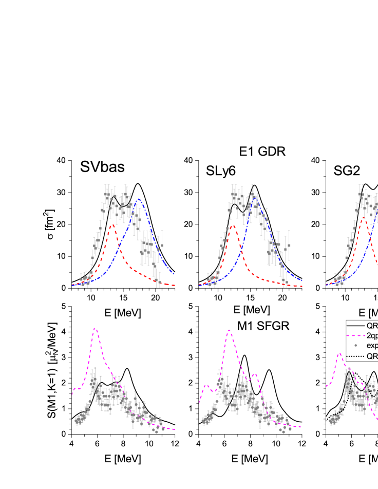
Figure 1: QRPA $E1$ photoabsorption (upper panels) and $M1$ SFGR (bottom panels) strengths in ¹⁵⁶Gd, calculated with the forces SVbas, SLy6, and SG2. For $E1$ GDR, the $K=0$ (left-side red dashed line) and $K=1$ (right-side blue dash-dot line) strengths are also depicted. For $M1$ SFGR, the unperturbed 2qp strength (magenta dashed line) is shown. For SG2, QRPA M1 strength is exhibited with (solid line) and without (dotted line) $\textbf{J}^{2}$ contribution. $E1$ GDR and $M1$ SFGR strengths use Lorentz weights with $\Delta$=2 MeV and 1 MeV, respectively. The strengths are compared with the photoabsorption data for $E1$ GDR Gur_exp81 and $(p,p^{\prime})$ data for $M1$ SFGR Wor_exp94 .

3 Results and discussion

3.1 $E1$ and $M1$ giant resonances

As a first step, we apply SVbas, SLy6 and SG2 to describe the IV $E1$ GDR and $M1$ SFGR. In Fig. 1, the calculated strength functions (7) and (8) are compared with the photoabsorption data for $E1$ GDR Gur_exp81 and $(p,p^{\prime})$ data for $M1$ SFGR Wor_exp94 . As discussed above, E1 and $M1$ strengths use different Lorentz averaging parameters: $\Delta$=2 MeV and 1 MeV, respectively. The $(p,p^{\prime})$ data Wor_exp94 are given in arbitrary units. So, in this case, not the absolute scale but the distribution of strength is of interest. The $(p,p^{\prime})$ reaction excites spin-flip and not orbital M1 strength Har01 . So the calculations for SFGR are performed with $g^{q}_{l}$=0.

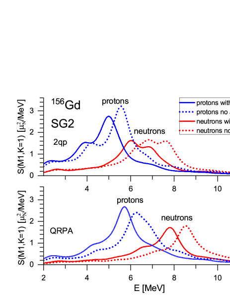
Figure 2: SG2 2qp (upper panel) and QRPA (bottom panel) proton and neutron spin M1 strength functions in ¹⁵⁶Gd, calculated with and without $\textbf{J}^{2}$-impact.

In the upper panels of Fig. 1, we present GDR branches $K=0$ and $K=1$ and the total strength. In general, all three Skyrme forces (with some preference for SLy6) give a nice description of GDR, including its deformation splitting into $K=0$ and $K=1$ branches. A small overestimation of the peak height of the $K=1$ branch can be explained by insufficient smoothing. The $K=1$ branch is located at a higher energy than $K=0$ and so should acquire more broadening from CCC. This could be simulated by an energy dependent folding width which we avoid here to keep the analysis simple. SG2 calculations for GDR are performed with $\textbf{J}^{2}$-term. As we checked, the impact of this term on GDR is negligible.

The bottom panels of Fig. 1 show the $K=1$ branch of $M1$ strength, responsible for the SFGR Har01 ; Hei10 ; Ves_PRC09 ; Nes_JPG10 , and $(p,p^{\prime})$ experimental data Wor_exp94 . Note that, in the recent FAM study Sasaki23 , the calculated and experimental distributions of M1 strength were not compared. Fig. 1 demonstrates that, in accordance to experiment Wor_exp94 , our calculated M1 strengths exhibit two large peaks produced by proton and neutron spin-orbit excitations. The origin of these peaks is illustrated in Fig. 2 where the separate proton and neutron spin ($g^{p}_{l}=g^{n}_{l}=0$) M1 QRPA strengths are depicted for 2qp and QRPA cases. It is known that unperturbed 2qp spin-flip proton and neutron excitations are determined by spin-orbit interaction $V_{so}\propto(\textbf{l}\cdot\textbf{s})$ where l and s are orbital moment and spin of the nucleon. In ¹⁵⁶Gd, the number of neutrons $N$ is much larger than number of protons $Z$. So, as compared with protons, neutrons occupy a higher valence quantum shell with a larger orbital moments $l$. This leads to a larger neutron spin-orbit splitting and so to a higher neutron spin-flip energy. Fig. 2 shows that indeed the neutron spin-flip M1 mode has a higher energy than the proton one. The proton peak is higher because $|g^{p}_{s}|>|q^{n}_{s}|$. The residual interaction upshifts M1 strength but still keeps the two-peak proton-neutron gross structure. A detail discussion of the proton-neutron gross structure of SFGR can be found elsewhere Hei10 ; Ves_PRC09 ; Nes_JPG10 .

Figure 3: The calculated (SVbas, SLy6, SG2) $K=0$, $K=1$ and total low-energy $E1$ strengths in ¹⁵⁶Gd as compared with $E1$ experimental data Tamkas_NPA19 .

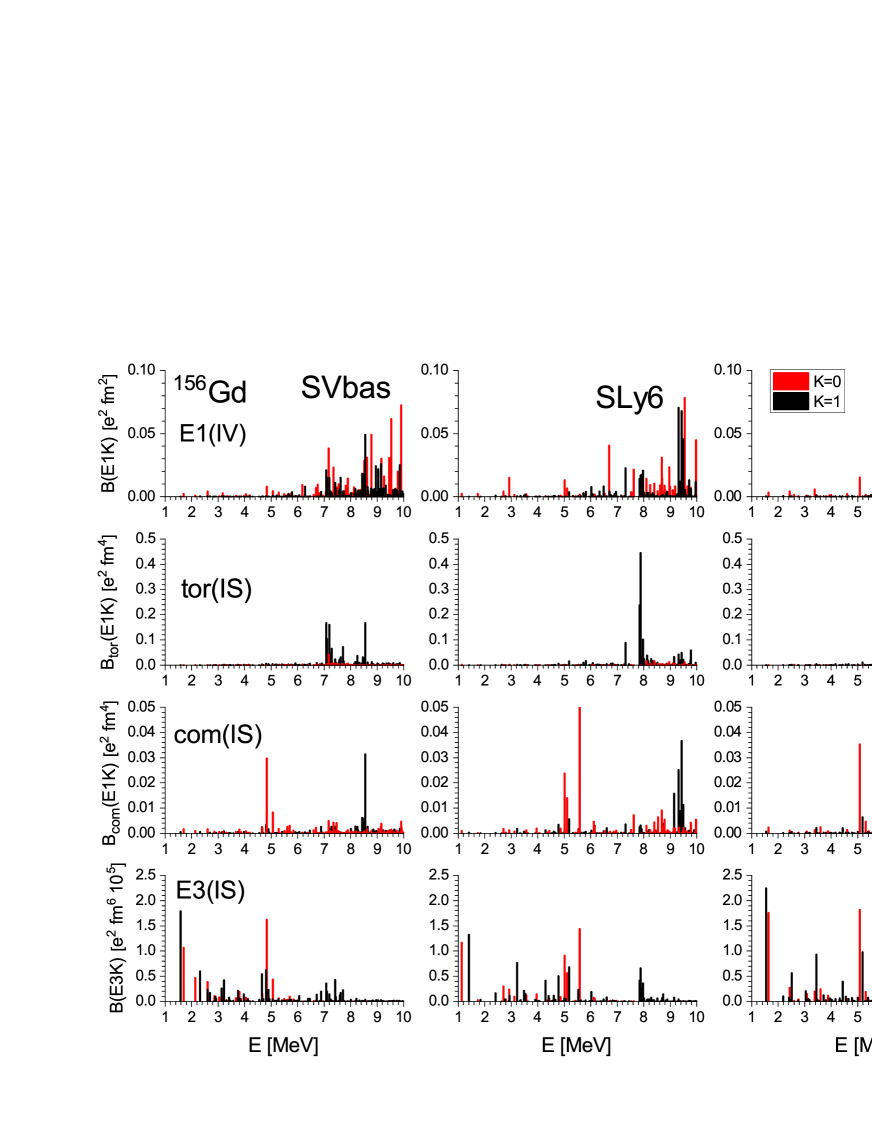
Figure 4: $K=0$ (red) and $K=1$ (black) branches of isovector $E1$ and isoscalar toroidal, compression and octupole strengths in ¹⁵⁶Gd, calculated with the forces SVbas, SLy6 and SG2.

As seen from bottom panels of Fig. 1, all Skyrme forces well describe the energy difference $\Delta E\approx$ 2.1 MeV between M1 peaks. At the same time, energies of $M1$ peaks are overestimated by 0.7-0.8 MeV (SVbas), 1.8-2.0 MeV (SLy6) and 0.7-0.9 MeV (no $\textbf{J}^{2}$ in SG2). Following previous studies Ves_PRC09 ; Nes_JPG10 , the peak energies are mainly determined by two factors: single-particle spin-orbit splitting and upshift due to the IV residual interaction in the spin channel of Skyrme functional. The latter effect is seen by comparison of unperturbed two-quasiparticle (2qp) and QRPA $M1$ strengths in Fig. 1. It is known that IS (IV) residual interaction leads to the energy downshift (upshift) of the strength. In Fig. 1 we see a significant upshift of M1 spin-flip strength, which points to the dominant impact of IV residual interaction. The impact of IV spin-spin interaction in Fig. 1 is obviously too strong and CCC will hardly help to correct the SFGR energy. However, if we include $\textbf{J}^{2}$-term, as done for SG2, then a necessary downshift of M1 strength is obtained and a good agreement with the experiment is achieved. So our results indicate a need for $\textbf{J}^{2}$ contribution even if this impact is limited by central exchange contribution.

The impact of $\textbf{J}^{2}$-term is additionally inspected for SG2 in Fig.2. We see that this term leads to a considerable change already in 2qp proton and neutron strengths, i.e. at the mean-field stage. Namely, we get a strong downshift of both proton and neutron peaks. Instead, the $\textbf{J}^{2}$ impact to the residual interaction is of a minor importance. Note that these results should be considered as preliminary. First of all, inclusion of the true tensor interaction with the corresponding refit of the force parameters can be important Ves_PRC09 ; Nes_JPG10 ; CS_PLB07 ; Les_PRC07 ; Bender_PRC09 . Further, the present SG2 results should be checked by calculations with other Skyrme parametrizations, which we leave to a future work. Anyway, our calculations show that a thorough test of spin-isospin parameters of the Skyrme functional by SFGR data for various nuclei is desirable. Note that, in previous studies CS_PLB07 ; Les_PRC07 ; Bender_PRC09 , the impact of $\textbf{J}^{2}$-term was mainly tested by description of single-particle spectra, in particular of spin-orbit splitting of single-particle levels. However, single-particle spectra are sensitive to many factors and, in this sense, are not optimal for $\textbf{J}^{2}$ tests. Instead, the energy and two-peak gross-structure of SFGR are more stable characteristics and so are more suitable for the tests.

An additional analysis can be done in terms of IS and IV Landau-Migdal spin-isospin parameters $g_{0}$ and $g_{0}^{\prime}$ shown in Table 1. SG2 values are obtained with $\textbf{J}^{2}$, otherwise, we have $g_{0}$=0.8 and $g_{0}^{\prime}$=1.2. We see that SVbas, SLy6 and SG2 have different strengths of IS and IV residual interactions in the spin-isospin channel. Nevertheless, despite significant variations in the interaction, SVbas, SLy6 and SG2 (no $\textbf{J}^{2}$) significantly overestimate the SFGR energy. The presence of IS interaction in SLy6 and SG2 (no $\textbf{J}^{2}$) does not improve the SFGR description. The latter looks reasonable since IV spin g-factor $g_{s}^{IV}=g_{s}^{p}-g_{s}^{n}$=6.24 is much larger than IS spin g-factor $g_{s}^{IS}=g_{s}^{p}+g_{s}^{n}$=1.35. So IS fraction of SFGR should be very small even in the case of the significant IS spin-spin residual interaction. Altogether, SFGR is mainly governed by IV residual interaction and does not suit for manifestation of IS one. However, IS spin-spin residual interaction can sometimes lead to local effects in M1 strength function, see Nes_JPG10 ; Paar_PRC20 for details.

Table 3: Calculated and experimental Tamkas_NPA19 summed $B(E1)$ strengths (in $\rm{e^{2}fm^{2}}$) at 3.1 - 6.2 MeV in ¹⁵⁶Gd.

force	$K=0$	$K=1$	total
SVbas	0.040	0.014	0.054
SLy6	0.030	0.028	0.058
SG2	0.042	0.008	0.050
exper. Tamkas_NPA19			0.073

3.2 Low-energy conventional, toroidal and compression $E1$ strengths

Figure 3 shows $E1$ strengths for excitations at 1.5 - 6.5 MeV, calculated with the forces SVbas, SLy6 and SG2 (with $\textbf{J}^{2}$). Note that NRF experiment Tamkas_NPA19 covers the energy region 3.1-6.2 MeV. We see that, in agreement with this experiment, all three Skyrme forces produce many QRPA states in the range 3.1-6.2 MeV. Most of the strength comes from the $K=0$ branch. This could be a consequence of the deformation splitting of the low-energy E1 strength, when $K=0$ branch is downshifted from the PDR energy region and becomes dominant at $E<$ 6 MeV.

Following Table 3, the calculated summed $E1$ strength is in acceptable agreement with data Tamkas_NPA19 . A small underestimation of the experimental strength can be explained by omitting the CCC which can somewhat redistribute $E1$ strength. For some states, our QRPA calculations give appreciably large $B(E1)$ values which are not seen in data Tamkas_NPA19 . This can be again explained by missing CCC. In general, all three applied Skyrme forces produce rather similar results. Following Fig. 1, the PDR region (5-9 MeV) in ¹⁵⁶Gd lies safely below GDR. Fig. 3 demonstrates a concentration of $E1$ strength at the low-energy part of this energy range. The summed low-lying $E1$ strength is given in Table 4.

The E1 (IV) $K=0$ and $K=1$ branches are exhibited at a wider energy range in upper panels of Fig. 4. The figure also includes IS toroidal E1, compression E1 and E3 strengths. The later is calculated with $e_{\text{eff}}^{p}=e_{\text{eff}}^{n}=$1. It is seen that all three Skyrme forces give similar results. Like in our previous studies for spherical Rep_PRC13 ; Rep_EPJA19 and deformed Nest_PAN16 ; Rep_EPJA17 ; 172Yb_E1tor ; Ne_PRL18 nuclei, toroidal states lie in the PDR energy region 7-10 MeV. Moreover, in accordance with earlier studies for deformed nuclei, the toroidal resonance is mainly presented in $K=1$ branch.

Table 4: Calculated summed $B(E1)$ (in $\rm{e^{2}fm^{2}}$), for $K=0,1$ and total cases at the PDR energy region 5-9 MeV in ¹⁵⁶Gd.

force	$K=0$	$K=1$	total
SVbas	0.34	0.34	0.68
SLy6	0.25	0.18	0.43
SG2	0.32	0.21	0.53

Figure 5: SVbas isoscalar current transition densities for $K^{\pi}=0^{-}$ states at 1.69 MeV (left) and 4.8 MeV (right) in ¹⁵⁶Gd. The scale of arrows in the left panel is twice larger than in the right panel. The solid line marks the nucleus boundary.

Figure 6: The calculated (SVbas, SLy6, SG2) orbital, spin, and total low-energy $M1$ strengths in ¹⁵⁶Gd as compared with $M1$ experimental data Tamkas_NPA19 .

In Fig. 4, the compression strength is much weaker than toroidal one. The compression mode demonstrates a clear deformation splitting typical for electric giant resonances in prolate nuclei. Namely, $K=0$ strength lies generally lower than $K=1$ one. Furthermore, unlike the upper panel of Fig. 4 for IV E1 strength, the compression IS E1 strength is not distributed among many dipole states but mainly concentrated in a pair of very collective peaks, e.g. at 4.8 MeV ($K=0$) and 8.6 MeV ($K=1$) for SVbas. A similar pattern takes place for SLy6 and SG2.

Note that energy region 4-9 MeV includes so-called Low-Energy Octupole Resonance (LEOR) Har01 ; LEOR_exp ; LEOR_MNS . Indeed, the bottom panel of Fig. 4 shows large IS octupole transition probabilities $B(E30)$ and $B(E31)$ for $I^{\pi}K=3^{-}0$ and $3^{-}1$ states. In deformed ¹⁵⁶Gd, the dipole and octupole modes should be mixed and this is clearly seen from comparison of the panels with compression dipole and octupole IS modes. The mixing depends on the structure of the state. For example, in SVbas calculations, the collective basically octupole $K=0$-states at 1.7 and 4.8 MeV have negligible and significant E1 compression fractions, respectively.

Mainly octupole character of 4.8-MeV state is confirmed by Fig. 5 where convective current transition density (CTD) $\delta\vec{j}(x,z)$ (see the definition in refs. Rep_EPJA17 ; Rep_EPJA19 ; Ne_PRC19 ) in z-x plane for 1.7-MeV and 4.8-MeV states are compared. The lengths of arrows $\delta\vec{j}(x,z)$ are properly scaled for the convenience of visibility. Following our analysis, both 1.7-MeV and 4.8-MeV states are mainly IS. Their CTD are rather similar and well match a typical octupole flow (see for comparison Fig. 10 in ref. Se83 for $3^{-}$-state in ²⁰⁸Pb). So 4.8-MeV state is basically octupole. At the same time, its flow somewhat reminds a pattern for the high-energy compression mode: the motion in pole regions against the quasi-static central part creates compression and decompression areas in the interface of moving and static parts. The similarity between E3 and compression E1 flows is not surprising since both modes are produced by similar shell transitions and have a similar radial dependence $r^{3}$.

The same analysis shows that SVbas $K=1$ state at 8.5 MeV has even more complicated composition.

The significant dipole-octupole mixture found in this study points that calculations for electric dipole $K=0,1$ states in deformed nuclei should take into account both dipole and octupole residual interactions. This was also found in the previous Skyrme QRPA studies for Nd and Sm isotopes Yoshida_PRC13 and highly deformed light nuclei Ne_PRC19 ; Ads21 . Note that, in schematic QRPA calculations for dipole states in ¹⁵⁶Gd Guliev20 , the octupole residual interaction was omitted.

3.3 Low-energy orbital and spin-flip $M1$ strengths

In Fig. 6, the calculated orbital, spin and total (orbital + spin) low-energy $M1(K=1)$ strengths in ¹⁵⁶Gd are compared with NRF $M1$ experimental data at 2.95-6.25 MeV Tamkas_NPA19 . SG2 results are obtained taking into account $\textbf{J}^{2}$-term. Note that NRF measurements should embrace both orbital and spin-flip M1 strengths. The calculations show a wide fragmentation of $M1$ strengths throughout the whole interval 1-7 MeV. In the OSR energy region 3-4 MeV, the calculated orbital strength is locally concentrated in accordance with NRF data Tamkas_NPA19 .h e properties of some selected calculated states are given in Table 5.

Table 5: Properties of particular QRPA low-energy $K^{\pi}=1^{+}$ states in ¹⁵⁶Gd: excitation energy $E$, orbital, spin and total $B(M1)$-values, and main proton (pp) and neutron (nn) components (Nillson quantum numbers and contribution in $\%$ to the state norm).

Force	E [MeV]	$B(M1)\;[\mu^{2}_{N}]$			main 2qp components
		orb	spin	total	$[N,n_{z},\Lambda]_{1},[N,n_{z},\Lambda]_{2}$	$\%$
SVbas	2.21	0.03	0.39	0.21	pp $[411\downarrow,411\uparrow]$	99
	3.23	0.92	0.10	1.63	nn $[521\uparrow,530\uparrow]$	39
					pp $[402\uparrow,411\uparrow]$	15
SLy6	2.46	0.07	0.32	0.09	pp $[411\downarrow,411\uparrow]$	98
	3.33	1.76	0.20	3.10	pp $[532\uparrow,541\uparrow]$	41
					nn $[521\uparrow,530\uparrow]$	39
SG2	2.35	0.02	0.34	0.20	pp $[411\downarrow,411\uparrow]$	99
	2.87	0.82	0.14	1.64	pp $[532\uparrow,541\uparrow]$	48
					nn $[642\uparrow,651\uparrow]$	47

Table 6: Calculated orbital, spin and total strength summed B(M1) (in $\mu^{2}_{N}$) in OSR region 2.5-4 MeV as compared with experimental data for ¹⁵⁶Gd and ¹⁵⁸Gd.

force	orb	spin	total	R
SVbas	1.89	0.52	3.57	1.48
SLy6	2.31	0.38	5.59	2.08
SG2	2.15	0.48	3.74	1.42
exper. Tamkas_NPA19			3.08
exper. Pitz_exp ; Enders_PRC05			2.73(56)
exper. 158Gd Pitz_exp ; Enders_PRC05			3.71(59)

Table 6 shows that, for SVbas and SG2, the summed M1 strength at OSR energy region 2.5-4 MeV somewhat exceeds the experimental values for ¹⁵⁶Gd Tamkas_NPA19 ; Pitz_exp ; Enders_PRC05 but agrees with the measurements for the neighbor nucleus ¹⁵⁸Gd Tamkas_NPA19 ; Pitz_exp ; Enders_PRC05 . Perhaps, a better agreement can be obtained after incorporation of CCC. Anyway, already at QRPA level, the agreement is quite acceptable.

Following Fig. 6 and Table 5, the calculated spin-flip mode in the OSR energy range is rather weak, and so $M1$ strength here is mainly orbital. Nevertheless, a small spin fraction is important for the estimation of the total $M1$ strength. Fig. 6 and Table 6 show a large constructive interference of the orbital and spin fractions ($B(M1)_{\rm tot}>B(M1)_{\rm orb}+B(M1)_{\rm spin}$). The interference can be estimated by the factor

$$R=\frac{B(M1)_{\rm tot}}{B(M1)_{\rm orb}+B(M1)_{\rm spin}}$$ (10)

where $R=1,>1,<1$ for zero, constructive and destructive interference. Table  6 shows that, due to the interference, the total $M1$ strength at 2.5-4 MeV becomes 1.5-2 times larger than the pure orbital strength.

Some time ago so called $M1$ ”spin scissors” mode (located just below the OSR) was predicted in deformed nuclei within macroscopic Wigner function moments approach Bal_PRC18 ; Bal_PAN20 . The microscopic Skyrme QRPA analysis for ^160,162,164Dy and ²³²Th Nest_PRC_SSR ; Nest_PAN_SSR has shown that, indeed, some low-energy spin-flip states can exist in some nuclei. However these states are usually not collective and their current fields deviate from the macroscopic spin-scissor flow. As seen in Fig. 6 and Table 5, such low-energy spin-flip states can exist in deformed ¹⁵⁶Gd as well. They lie at 2.21 MeV (SVbas), 2.46 MeV (SLy6) and 2.35 MeV (SG2). Each such state is represented by one 2qp configuration of spin-flip character. SG2 calculations show that inclusion of $\textbf{J}^{2}$-term does not affect much these findings.

Table 7: Calculated and experimental Tamkas_NPA19 summed B(M1) values (in $\mu^{2}_{N}$) at 2.95 - 6.25 MeV in ¹⁵⁶Gd.

force	orb	spin	total
SVbas	4.21	2.72	6.89
SLy6	4.50	1.35	7.22
SG2	3.77	4.64	6.97
exper. Tamkas_NPA19			3.12

Fig. 6 shows a significant discrepancy between calculated and experimental $M1$ strengths at 4-6 MeV. The experimental strength Tamkas_NPA19 at this energy is almost absent while our calculations give significant orbital, spin and total $B(M1)$-values. Just for this reason, the calculated $M1$ strength summed at 2.95-6.25 MeV (6.9-7.2 $\mu^{2}_{N}$) significantly overestimates the experimental value 3.12 $\mu^{2}_{N}$ (see Table 7). Note that a large $M1$ strength at 4-6 MeV was observed in $(e,e^{\prime})$ reaction Richter90 ; Richter95 . Moreover, a significant spin-flip $M1$ strength at this energy range in ^156,158Gd was reported in Skyrme QRPA studies Sarr96 ; Sasaki23 . Our Skyrme QRPA calculations Nes_JPG10 and $(p,p^{\prime})$ data Wor_exp94 also give a significant spin-flip $M1$ strength at 4-6 MeV in the neighbor nucleus ¹⁵⁸Gd. Following our Fig. 1 and previous studies mentioned above, the interval 4-6 MeV in ^156,158Gd should include the proton fraction of SFGR and thus embrace an appreciable $M1$ strength. Inclusion of $\textbf{J}^{2}$-term in SG2 does not change this result. In this connection, the absence of $M1$ strength at 4-6 MeV in the NRF experiment for ¹⁵⁶Gd Tamkas_NPA19 looks questionable.

4 Conclusions

$E1$ and $M1$ excitations in deformed ¹⁵⁶Gd were simultaneously investigated within fully self-consistent QRPA calculations with Skyrme forces SVbas, SLy6 and SG2. In the $E1$ channel, the analysis covers low-lying $E1$ strength, called pygmy dipole resonance (PDR), giant dipole resonance (GDR), and low-energy toroidal and compression $E1$ excitations. In $M1(K=1)$ channel, we consider spin-flip giant resonance (SFGR), orbital scissors resonance (OSR), and low-energy spin-flip excitations.

The calculations well describe the energy and gross-structure (deformation splitting) of $E1$ GDR. In PDR energy region, we reasonably reproduce the summed $E1$ strength at 2.95-6.25 MeV, measured in the NRF experiment Tamkas_NPA19 . A dominance of $K=0$ strength over $K=1$ one at this energy range points out the deformation splitting of these $K$-branches. In agreement with our previous studies for deformed nuclei Rep_EPJA17 ; Nest_PAN16 ; 172Yb_E1tor ; Ne_PRL18 , the present calculations confirm the existence of the prominent toroidal $E1(K=1)$ resonance at PDR energy. Note that the vortical toroidal mode can affect irrotational PDR E1 strength and its impact on astrophysical applications. The compression low-energy E1 strength is weak and demonstrates a clear deformation splitting.

The calculations show a significant deformation-induced admixture of E3 mode (low-energy octupole resonance - LEOR Har01 ; LEOR_exp ; LEOR_MNS ) to dipole $K=$0,1 states. This means that analysis of low-energy E1 states in deformed nuclei should take into account both dipole and octupole residual interaction, which automatically occurs in self-consistent microscopic models. Note that the previous systematic study of electric dipole spectra in Gd isotopes within schematic QRPA Guliev20 omits the octupole residual interaction.

The calculations reveal a strong constructive interference of the orbital and spin $M1$ modes in OSR energy region. This is important for estimation of the summed OSR M1 strength.

For $M1$ SFGR, the proton-neutron gross structure, impact of the residual interaction and influence of central exchange $\textbf{J}^{2}$-term were analyzed. The dominance of IV residual interaction over the IS one was justified. The calculations well reproduce proton-neutron splitting of SFGR but overestimate energies of the proton and neutron $M1$ peaks. Following our calculations with SG2, this shortcoming can be cured by taking into account $\textbf{J}^{2}$-term. This result should be yet considered as preliminary since it was obtained without i) refit of entire SG2 parameters and ii) inclusion of non-central tensor forces. Anyway, it is shown that SFGR can be a valuable test for the impact of $\textbf{J}^{2}$-term.

Table 8: Skyrme parameters for forces SVbas, SLy6 and SG2.

Force	$t_{0}$	$t_{1}$	$t_{2}$	$t_{3}$	$t_{4}$	$x_{0}$	$x_{1}$	$x_{2}$	$x_{3}$	$\alpha$
SVbas	-1879	314	113	12527	125	0.259	-0.382	-2.82	0.123	0.3
SLy6	-2479	462	-449	13673	122	0.825	-0.465	-1.0	1.355	0.167
SG2	-2645	340	-42	15595	105	0.09	-0.059	1.43	0.060	0.167

Further, there was found a puzzling discrepancy between calculated and experimental Tamkas_NPA19 $M1$ strengths at 4-6 MeV. Following our calculations and previous theoretical Nes_JPG10 ; Sarr96 ; Sasaki23 and experimental Richter90 ; Richter95 ; Wor_exp94 work, this energy interval should host the proton branch of SFGR and so carry an impressive $M1$ strength. At the same time, the NRF experiment Tamkas_NPA19 delivers almost no $M1$ strength at 4-6 MeV. The reason of the discrepancy is yet unclear.

Appendix A Skyrme functional

The Skyrme functional has the form Ves_PRC09 ; Ben_RMP03 ; Stone_PPNP07

$$\mathcal{H}_{\mathrm{Sk}} = \frac{b_{0}}{2}\rho^{2}-\frac{b^{\prime}_{0}}{2}\sum\rho_{q}^{2}+\frac{b_{3}}{3}\rho^{\alpha+2}-\frac{b^{\prime}_{3}}{3}\rho^{\alpha}\sum\rho^{2}_{q}$$ (A.1)

$$+b_{1}(\rho\tau-\textbf{j}^{\;2})-b^{\prime}_{1}\sum(\rho_{q}\tau_{q}-\textbf{j}^{\;2}_{q})$$

$$-\frac{b_{2}}{2}\rho\Delta\rho+\frac{b^{\prime}_{2}}{2}\sum\rho_{q}\Delta\rho_{q}$$

$$-b_{4}(\rho\nabla\cdot\textbf{J}\!+\!(\nabla\!\times\!\textbf{j})\!\cdot\!\textbf{s})$$

$$-b^{\prime}_{4}\sum(\rho_{q}\nabla\cdot\textbf{J}_{q}\!+\!(\nabla\!\times\!\textbf{j}_{q})\!\cdot\!\textbf{s}_{q})$$

$$+\frac{\tilde{b}_{0}}{2}\textbf{s}^{\;2}-\frac{\tilde{b}^{\prime}_{0}}{2}\sum\textbf{s}_{q}^{\;2}+\frac{\tilde{b}_{3}}{3}\rho^{\alpha}\textbf{s}^{\;2}-\frac{\tilde{b}^{\prime}_{3}}{3}\rho^{\alpha}\sum\textbf{s}^{\;2}_{q}$$

$$-\frac{\tilde{b}_{2}}{2}\textbf{s}\!\cdot\!\Delta\textbf{s}+\frac{\tilde{b}^{\prime}_{2}}{2}\sum\textbf{s}_{q}\!\cdot\!\Delta\textbf{s}_{q}$$

$$+\tilde{b}_{1}(\textbf{s}\!\cdot\!\textbf{T}\!-\!\textbf{J}^{2})+\tilde{b}^{\prime}_{1}\sum(\textbf{s}_{q}\!\cdot\!\textbf{T}_{q}\!-\!\textbf{J}_{q}^{2}).$$

Here $b_{i}$, $b^{\prime}_{i}$, $\tilde{b}_{i}$, $\tilde{b}^{\prime}_{i}$ are the force parameters. The relation of these parameters with standard ones can be found in Refs. Ves_PRC09 ; Ben_RMP03 ; Stone_PPNP07 ; Bonche_NPA87 . Functional (A.1) includes time-even (nucleon $\rho_{q}$, kinetic-energy $\tau_{q}$, spin-orbit $\textbf{J}_{q}$) and time-odd (current $\textbf{j}_{q}$, spin $\textbf{s}_{q}$, spin kinetic-energy $\textbf{T}_{q}$) densities. The label $q\in\{p,n\}$ $q$ denotes protons and neutrons. Densities without index $q$, like $\rho=\rho_{p}+\rho_{n}$, denote total densities. The contributions with $b_{i}$ (i=0,1,2,3,4) and $b^{\prime}_{i}$ (i=0,1,2,3) are the standard terms responsible for ground state properties and electric excitations of even-even nuclei Ben_RMP03 . The isovector spin-orbit interaction is usually linked to the isoscalar one by $b^{\prime}_{4}=b_{4}$. The terms with $\tilde{b}_{i},\tilde{b}^{\prime}_{i}$ ($i$=0,1,2,3) represent the spin-isospin channel important for odd nuclei and magnetic modes in even-even nuclei. The last line of (A.1) includes tensor spin-orbit terms $\propto\tilde{b}_{1},\tilde{b}^{\prime}_{1}$ which can affect both mean-field ground-state properties and magnetic modes. In general, these terms embrace contributions from both central-exchange interaction and non-central tensor interaction CS_PLB07 ; Les_PRC07 ; Bender_PRC09 . In our calculations, $\textbf{J}^{2}$ is taken into account only for SG2 and only with central exchange contribution. In this case, $\tilde{b}_{i}$ and $\tilde{b}^{\prime}_{i}$ are fully expressed through the standard Skyrme parameters $t_{1},t_{2},x_{1},x_{2}$ (see Eqs. (A.13)-(A.14) below) and have the values ${\tilde{b}}_{1}$=-40.1, ${\tilde{b}}^{\prime}_{1}$=-47.8.

The parameters $b_{i}$, $b^{\prime}_{i}$, $\tilde{b}_{i}$, $\tilde{b}^{\prime}_{i}$ are related with standard Skyrme parameters as Ves_PRC09 ; Ben_RMP03 ; Stone_PPNP07 ; Bonche_NPA87 .

$$b_{0} = t_{0}(1+\frac{1}{2}x_{0}),$$ (A.2)

$$b^{\prime}_{0} = t_{0}(\frac{1}{2}+x_{0}),$$ (A.3)

$$b_{1} = \frac{1}{4}[t_{1}(1+\frac{1}{2}x_{1})+t_{2}(1+\frac{1}{2}x_{2})],$$ (A.4)

$$b^{\prime}_{1} = \frac{1}{4}[t_{1}(\frac{1}{2}+x_{1})-t_{2}(\frac{1}{2}+x_{2})],$$ (A.5)

$$b_{2} = \frac{1}{8}[3t_{1}(1+\frac{1}{2}x_{1})-t_{2}(1+\frac{1}{2}x_{2})],$$ (A.6)

$$b^{\prime}_{2} = \frac{1}{8}[3t_{1}(\frac{1}{2}+x_{1})+t_{2}(\frac{1}{2}+x_{2})],$$ (A.7)

$$b_{3} = \frac{1}{4}t_{3}(1+\frac{1}{2}x_{3}),$$ (A.8)

$$b^{\prime}_{3} = \frac{1}{4}t_{3}(\frac{1}{2}+x_{3}),$$ (A.9)

$$b_{4} = b^{\prime}_{4}=\frac{1}{2}t_{4},$$ (A.10)

$${\tilde{b}}_{0} = \frac{1}{2}t_{0}x_{0},$$ (A.11)

$${\tilde{b}}^{\prime}_{0} = \frac{1}{2}t_{0}$$ (A.12)

$${\tilde{b}}_{1} = \frac{1}{8}(t_{1}x_{1}+t_{2}x_{2}),$$ (A.13)

$$\tilde{b}^{\prime}_{1} = -\frac{1}{8}(t_{1}-t_{2}),$$ (A.14)

$${\tilde{b}}_{2} = \frac{1}{16}(3t_{1}x_{1}-t_{2}x_{2}),$$ (A.15)

$$\tilde{b}^{\prime}_{2} = \frac{1}{16}(3t_{1}+t_{2}),$$ (A.16)

$${\tilde{b}}_{3} = \frac{1}{8}t_{3}x_{3},$$ (A.17)

$${\tilde{b}}^{\prime}_{3} = \frac{1}{8}t_{3}.$$ (A.18)

As seen from Table 8, Skyrme parameters $t_{1},t_{2},x_{1},x_{2}$, entering $\textbf{J}^{2}$ parameters ${\tilde{b}}_{1}$ and ${\tilde{b}}^{\prime}_{1}$, are rather different for SVbas, SLy6 and SG2.

References

- (1) M. N. Harakeh and A. van der Woude, Giant Resonances (Clarendon Press, Oxford, 2001).
- (2) N. Paar, D. Vretenar, E. Khan, and G. Colò, Rep. Prog. Phys. 70, 691 (2007).
- (3) K. Heyde, P. von Neumann-Cosel, and A. Richter, Rev. Mod. Phys. 82, 2365 (2010).
- (4) D. Savran, T. Aumann, and A. Zilges, Prog. Part. Nucl. Phys. 70, 210 (2013).
- (5) A. Bracco, E.G. Lanza, and A. Tamii, Prog. Part. Nucl. Phys. 106, 360 (2019).
- (6) P. Klupfel, P.-G. Reinhard, T.J. Burvenich, J.A. Maruhn, Phys. Rev. C 79, 034310 (2009).
- (7) W. Kleinig, V.O. Nesterenko, J. Kvasil, P.-G. Reinhard and P. Vesely, Phys. Rev. C 78, 044313 (2008).
- (8) N. Lo Iudice and F. Palumbo, Phys. Rev. Lett. 41, 1532 (1978).
- (9) D. Bohle, A. Richter, W. Steffen, A. Diepernik, N. Lo Iudice, F. Palumbo, O. Scholten, Phys. Lett. B 137, 27 (1984).
- (10) N. Pietralla, P. von Brentano, and A.F. Lisetskiy, Prog. Part. Nucl. Phys. 60, 225 (2008).
- (11) Li-Gang Cao, G. Colò, H. Sagawa, P.F. Bortignon, and L. Sciacchitano, Phys. Rev. C 80, 064304 (2009).
- (12) P. Vesely, J. Kvasil, V.O. Nesterenko, W. Kleinig, P.-G. Reinhard, and V.Yu. Ponomarev, Phys. Rev. C 80, 031302 (2009).
- (13) V.O. Nesterenko, J. Kvasil, P. Vesely, W. Kleinig, P.-G. Reinhard, and V.Yu. Ponomarev, J. Phys. G: Nucl. Part. Phys. 37, 064034 (2010).
- (14) S. Goriely, S. Hilaire, S. Péru, M. Martini, I. Deloncle, and F. Lechaftois, Phys. Rev. C 94, 044306 (2016).
- (15) V. Tselyaev, N. Lyutorovich, J. Speth, P.-G. Reinhard, and D. Smirnov, Phys. Rev. C 99, 064329 (2019).
- (16) G. Kružić, T. Oishi, D. Vale and N. Paar, Phys. Rev. C 102, 044315 (2020).
- (17) F. Mercier, J.-P. Ebran, and E. Khan, Phys. Rev. C 107, 034309 (2023).
- (18) V.O. Nesterenko, J. Kvasil, A. Repko, W. Kleinig, and P.-G. Reinhard, Phys. At. Nuclei 79, 842 (2016).
- (19) J. Kvasil, V.O. Nesterenko,W. Kleinig, P.-G. Reinhard, and P. Vesely, Phys. Rev. C 84, 034303 (2011).
- (20) A. Repko, P.-G. Reinhard, V.O. Nesterenko, and J. Kvasil, Phys. Rev. C 87, 024305 (2013).
- (21) A. Repko, J. Kvasil, V.O. Nesterenko, and P.-G. Reinhard, Eur. Phys. J. A 53, 221 (2017).
- (22) A. Repko, V.O. Nesterenko, J. Kvasil, and P.-G. Reinhard, Eur. Phys. J. A 55, 242 (2019)
- (23) V.O. Nesterenko, A. Repko, J. Kvasil, and P.-G. Reinhard, Phys. Rev. C 100, 064302 (2019).
- (24) E.B. Balbutsev, I.V. Molodtsova, and P. Schuck, Phys. Rev. C 97, 044316 (2018).
- (25) E.B. Balbutsev, I.V. Molodtsova, and P. Schuck, Phys. Atom. Nucl. 83, 212 (2020).
- (26) V.O. Nesterenko, P.I. Vishnevskiy, J. Kvasil, A. Repko, and W. Kleinig, Phys. Rev. C 103, 064313 (2021).
- (27) V.O. Nesterenko, P.I. Vishnevskiy, A. Repko and J. Kvasil, Phys. At. Nuclei, 85, 858 (2022).
- (28) G.M. Gurevich, L.E. Lazareva, V.M. Mazur, S.Yu. Merkulov, G.V. Solodukhov, and V.A. Tyutin, Nucl. Phys. A 351, 257 (1981).
- (29) H.H. Pitz, U.E.P. Berg, R.D. Heil, U. Kneissl, R. Stock, C. Wesselborg, and P. von Brentano, Nucl. Phys. A 492, 411 (1989).
- (30) A. Richter, Nucl. Phys. A 507, 99c (1990).
- (31) A. Richter, Prog. Part. Nucl. Phys. 34, 261 (1995).
- (32) H.J. Wörtche, Ph.D. thesis, Technischen Hochschule Darmstadt, Germany, 1994.
- (33) M. Tamkas, E. Aciksoz, J. Issak, T. Beck, N. Benouaret, M. Bhike, I.Boztosun, A. Durusoy, U. Gayer, Krishichayan, B.Loher, N. Pietralla, D. Savran , W.Tornow, V. Werner, A.Zilges, M. Zweidinger, Nucl. Phys. A 987, 79 (2019).
- (34) R. Nojarov and A. Faessler, Z. Phys. A: Atomic Nuclei 336, 151 (1990).
- (35) P. Sarriguren, E. Moya de Guerra, and R. Nojarov, Phys. Rev. C 54, 690 (1996).
- (36) E. Guliyev, H. Quliyev, and A.A. Kuliev, J. Phys. G: Nucl. Part. Phys. 47, 115107 (2020).
- (37) V.G. Soloviev, A.V. Sushkov, N.Yu. Shirikova, and N. Lo Iudice, Nucl. Phys. A 600, 155 (1996).
- (38) V.G. Soloviev, A.V. Sushkov and N.Yu. Shirikova, Phys. Part. Nucl. 31, n. 4, 385 (2000).
- (39) H. Sasaki, T. Kawano and I. Stetcu, Phys. Rev. C 107, 054312 (2023).
- (40) E. Chabanat, P. Bonche, P. Haensel, J. Meyer, and R. Schaeffer, Nucl. Phys. A 635, 231 (1998).
- (41) A. Repko, J. Kvasil, V. O. Nesterenko, and P. G. Reinhard, arxiv:1510.01248 (nucl-th).
- (42) A. Repko, Ph.D. thesis, Charles University, Prague, 2015; arXiv:1603.04383 (nucl-th).
- (43) A. Repko, J. Kvasil, and V.O. Nesterenko, Phys. Rev. C 99, 044307 (2019).
- (44) J. Kvasil, A. Repko, and V.O. Nesterenko, Eur. Phys. J. A 55, 213 (2019).
- (45) L.M. Donaldson, J. Carter, P. von Neumann-Cosel, V.O. Nesterenko, R. Neveling, P.-G. Reinhard, I.T. Usman, P. Adsley, C.A. Bertulani, J.W. Brümmer, E.Z. Buthelezi, G.R.J. Cooper, R.W. Fearick, S.V. Förtsch, H. Fujita, Y. Fujita, M. Jingo, N.Y. Kheswa, W. Kleinig, C.O. Kureba, J. Kvasil, M. Latif, K.C.W. Li, J.P. Mira, F. Nemulodi, P. Papka, L. Pellegri, N. Pietralla, V.Yu. Ponomarev, B. Rebeiro, A. Richter, N.Yu. Shirikova, E. Sideras-Haddad, A.V. Sushkov, F.D. Smit, G.F. Steyn, J.A. Swartz, and A. Tamii, Phys. Rev. C 102, 064327 (2020).
- (46) H. Pai, T. Beck, J. Beller, R. Beyer, M. Bhike, V. Derya, U. Gayer, J. Isaak, Krishichayan, J. Kvasil, B. Lȯher, V. O. Nesterenko, N. Pietralla, G. Martínez-Pinedo, L. Mertes, V. Yu. Ponomarev, P.-G. Reinhard, A. Repko, P.C. Ries, C. Romig, D. Savran, R. Schwengner, W. Tornow, V. Werner, A. Zilges, and M. Zweidinger, Phys. Rev. C 93, 014318 (2016).
- (47) J. Speth, P.-G. Reinhard, V. Tselyaev, and N. Lyutorovich, Phys. Rev. C 102, 054332 (2020).
- (48) M. Bender, P.-H. Heenen, and P.-G. Reinhard, Rev. Mod. Phys. 75, 121 (2003).
- (49) J. R. Stone and P.-G. Reinhard, Prog. Part. Nucl. Phys. 58, 587 (2007).
- (50) N. Van Giai and H. Sagawa, Phys. Lett. B 106, 379 (1981).
- (51) V.O. Nesterenko, W. Kleinig, J. Kvasil, P. Vesely, and P.-G. Reinhard, Int. J. Mod. Phys. E 17 89 (2008).
- (52) A.B. Migdal, Theory of Finite Fermi Systems and Application to Atomic Nuclei (Wiley, New York, 1967).
- (53) L.D. Landau, E.M. Lifshitz, and L. P. Pitajevski, Course of Theoretical Physics 9 — Statistical Physics (Pergamon, Oxford, 1980).
- (54) G. Colò, H. Sagawa, S. Fracasso and P.F. Bortignon, Phys. Lett. B, 646, 227 (2007).
- (55) T. Lesinski, M. Bender, K. Bennaceur, T. Duguet, and J. Meyer, Phys. Rew. C 76, 014312 (2007).
- (56) M. Bender, K. Bennaceur, T. Duguet, P.-H. Heenen, T. Lesinski, and J. Meyer, Phys. Rev. C 80, 064302 (2009).
- (57) W. Satula, M. Zalewski, J. Dobaczewski, P. Olbratowski, M. Rafalski, T. R. Werner and R. A. Wyss, Int. J. Mod. Phys. E 18, 808 (2009).
- (58) P.-G. Reinhard, B. Schuetrumpf, and J.A. Maruhn, Comput. Phys. Commun. 258, 107603 (2021).
- (59) Database http://www.nndc.bnl.gov/nudat2/chartNuc.jsp
- (60) M. Bender, K. Rutz, P.-G. Reinhard, and J.A. Maruhn, Eur. Phys. J. A 8, 59 (2000).
- (61) P.-G. Reinhard, private communication.
- (62) D.J. Thouless and J.G. Valatin, Nucl. Phys. 31, 211 (1962).
- (63) J. Kvasil, A. Repko, V.O. Nesterenko, W. Kleinig, and P.-G. Reinhard, Int. J. Mod. Phys. E 21, 1250041 (2012).
- (64) J. Kvasil, V.O. Nesterenko, W. Kleinig, and P.-G. Reinhard, Phys. Scr. 89, 054023 (2014).
- (65) V.O. Nesterenko, A. Repko, J. Kvasil, and P.-G. Reinhard, Phys. Rev. Lett. 120, 182501 (2018).
- (66) K. Yoshida and T. Nakatsukasa, Phys. Rev. C 88, 034309 (2013).
- (67) P. Adsley, V.O. Nesterenko, M. Kimura, L.M. Donaldson, R. Neveling, J.W. Brümmer, D.G. Jenkins, N.Y. Kheswa, J. Kvasil, K.C.W. Li, D.J. Marín-Lámbarri, Z. Mabika, P. Papka, L. Pellegri, V. Pesudo, B. Rebeiro, P.-G. Reinhard, F. D. Smit, and W. Yahia-Cherif, Phys. Rev. C103, 044315 (2021).
- (68) H.H. Pitz, R.D. Heil, U. Kneissl, S. Lindenstruth, U. Seemann, R. Stock, C.Wesselborg, A. Zilges, P. von Brentano, S.D. Hoblit, and A. M. Nathan, Nucl. Phys. A 509, 587 (1990).
- (69) J. Enders, P. von Neumann-Cosel, C. Rangacharyulu, and A. Richter, Phys. Rev C 71, 014306 (2005).
- (70) J.M. Moss, D.H. Youngblood, C.M. Rozsa, D.R. Brown and J.D. Bronson, Phys. Rev. Lett. 37, 816 (1976)
- (71) L.A.Malov, V.O.Nesterenko and V.G.Soloviev, J. Phys. G: Nucl. Phys. 3 L219 (1977).
- (72) F.E. Serr, T.S. Dumitrescu, T. Suzuki and C.H. Dasso, Nucl. Phys. A 404, 359 (1983).
- (73) P. Bonche, H. Flocard and P.H. Heenen, Nucl. Phys. A 467, 115 (1987).