Optimal Rate of Kernel Regression
in Large Dimensions

Abstract

We perform a study on kernel regression for large-dimensional data (where the sample size $n$ is polynomially depending on the dimension $d$ of the samples, i.e., $n\asymp d^{\gamma}$ for some $\gamma>0$ ). We first build a general tool to characterize the upper bound and the minimax lower bound of kernel regression for large dimensional data through the Mendelson complexity $\varepsilon_{n}^{2}$ and the metric entropy $\bar{\varepsilon}_{n}^{2}$ respectively. When the target function falls into the RKHS associated with a (general) inner product model defined on $\mathbb{S}^{d}$, we utilize the new tool to show that the minimax rate of the excess risk of kernel regression is $n^{-1/2}$ when $n\asymp d^{\gamma}$ for $\gamma=2,4,6,8,\cdots$. We then further determine the optimal rate of the excess risk of kernel regression for all the $\gamma>0$ and find that the curve of optimal rate varying along $\gamma$ exhibits several new phenomena including the multiple descent behavior and the periodic plateau behavior. As an application, For the neural tangent kernel (NTK), we also provide a similar explicit description of the curve of optimal rate. As a direct corollary, we know these claims hold for wide neural networks as well.

Keywords kernel regression  $\cdot$ neural network  $\cdot$ high-dimensional statistics  $\cdot$ minimax rates

1 Introduction

Suppose we have observed $n$ i.i.d. samples $(X_{i},Y_{i})$ from a joint distribution $(X,Y)$ supported on $\mathbb{R}^{d+1}\times\mathbb{R}$. The regression problem, one of the most fundamental problems in statistics, aims to find a function $\hat{f}_{n}$ based on these samples such that the excess risk,

$$\left\|\hat{f}_{n}-f_{\star}\right\|_{L^{2}}^{2}=\mathbb{E}_{X}\left[\left(f_{\star}(X)-\hat{f}_{n}(X)\right)^{2}\right],$$

is small, where $f_{\star}(x)=\mathbf{E}[Y|x]$ is the regression function. Many non-parametric regression methods are proposed to solve the regression problem, such as polynomial splines [72], local polynomials [21, 71], the kernel methods [14, 15, 16], etc. When the dimension $d$ of data is small, these methods produce reasonable results; however, when $d$ is relatively large, the convergence rate of the excess risk can be extremely slow. What’s worse, though some additional assumptions such as low intrinsic dimensionality (that data falls into a subspace with dimension far smaller than $d$) and sparsity of features can improve the theoretical performance of certain non-parametric regression problems [2, 27], few successful real-world examples/applications have been reported. On the other hand, neural network methods have gained tremendous successes in many large-dimensional problems, such as computer vision [34, 42] and natural language processing [23]. For example, the ILSVRC competition [63] has a dataset of 1.2 million samples with a dimensionality of approximately 200K, while the pre-train dataset of the well-known language representation model, Bidirectional Encoder Representations from Transformers (BERT) [23], consists of 13 million samples with a dimensionality of approximately 400K.

Several groups of researchers tried to explain the superior performance of neural networks on large dimensional data from various aspects. However, the highly non-linear dynamic of the differential equation associated with the gradient descent/flow of training the neural network[32, 44, 61] makes the analysis on the dynamic of training the neural network notoriously hard. When the width of a neural network is sufficiently large, the training process falls into the ‘lazy regime’, i.e., its parameters/weights stay in a small neighborhood of their initial position during the training process [3, 25, 26, 47]. Since [38] observed that the time-varying neural network kernel (NNK) converges to a time-invariant neural tangent kernel (NTK) point-wisely as the width $m$ of the neural network $\rightarrow\infty$, it has been widely believed that the generalization ability of early-stopping kernel regression with NTK could be served as a proper surrogate of the generalization ability of neural networks in the ‘lazy regime’ [4, 36, 73]. Recently, a sequence of works [43, 45] further showed that the NNK uniformly converges to the NTK as the width $m\rightarrow\infty$ which rigorously justified this belief. Thus, understanding the generalization ability of the kernel regression (with respect to NTK) in large dimensions will help us understand the superior performance of (wide) neural networks.

Kernel regression (or regression over an RKHS), as a classical topic, has been studied since the 1990s. Most work imposes the polynomial eigenvalue decay assumption over a kernel $K$ (i.e., there exist constants $0<\mathfrak{c}\leq\mathfrak{C}<\infty$, such that the eigenvalues of the kernel satisfy $\mathfrak{c}j^{-\beta}\leq\lambda_{j}\leq\mathfrak{C}j^{-\beta}$ for some constant $\beta>1$) and assume that the target function $f_{\star}$ belongs to the RKHS associated with $K$ [14, 15, 50, 62]. They then showed that the minimax rate of the excess risk of regression over the corresponding RKHS is lower bounded by $n^{-{\beta}/({\beta+1})}$ and that some kernel methods (e.g., the kernel ridge regression and the early-stopping kernel regression) can produce estimators achieving this optimal rate. Thus, verifying that if an NTK satisfies the polynomial eigenvalue decay assumption and determining the eigenvalue decay rate of it becomes a natural strategy to discuss the generalization ability of the NTK ( or equivalently, the wide neural networks ) regression. When the NTK is defined on sphere $\mathbb{S}^{d}$, it is an inner product kernel. Hence, the eigenvalues of NTK can be obtained through a detailed calculation with the help of the spherical harmonic polynomials. It is shown in [10, 11] that when $d$ is fixed, the eigenvalues of the NTK defined on $\mathbb{S}^{d}$ polynomially decayed at rate $({d+1})/{d}$. When the domain is other than a sphere, [43, 45] further illustrated that the eigenvalues decay rate of NTK on any bounded open set in $\mathbb{R}^{d}$ is still $({d+1})/{d}$. Some works then claimed that the optimal tuned neural network on $\mathbb{S}^{d}$ or on any bounded open set in $\mathbb{R}^{d}$ can achieve the optimal rate $n^{-({d+1})/({2d+1})}$ [36, 43, 45].

When dimension $d$ is large, much less is known about convergence rate of the excess risk of kernel methods. There are several works devoted to the high-dimensional setting where $n\asymp d$. For example, motivated by the linear approximation of kernel matrices in high dimensional data proposed by [39], [48] provided an upper bound on the excess risk of kernel interpolation and claimed that kernel interpolation generalizes well in high dimensions. Similar results for kernel ridge regression are proven in [51]. These results are widely interpreted as evidence of the benign overfitting phenomenon (e.g., [9, 11, 52, 65]): overfitted models can still generalize well. Building on the work of [48], the benign overfitting phenomenon has been extensively investigated in the literature, and we referred to [8, 13, 33, 60, 75] for details. There is another line of research considering the large dimensional setting where $n\asymp d^{\gamma}$ for some ${\gamma}>0$. For example, [30] studied the square-integrable function space on the sphere $\mathbb{S}^{d}$ and proved that when ${\gamma}$ is a non-integer, kernel ridge regression is consistent if and only if the regression function is a polynomial with a fixed degree $\leq\gamma$. Inspired by the techniques presented in [30], several follow-up works extended the results to different settings [1, 29, 31, 54, 55, 59]. Additionally, [24] established an upper bound for kernel methods with specific kernels when ${\gamma}$ is an integer. All these inspirational works hint that determining the convergence rate of kernel regression in large dimensions is a hard but fruitful question.

In this paper, we consider the generalization ability of kernel regression, especially kernel regression with inner product kernel defined on sphere $\mathbb{S}^{d}$, with respect to large-dimensional data where $n\asymp d^{\gamma}$. More precisely, assuming the target function $f_{\star}\in\mathcal{H}^{\mathtt{in}}$, the RKHS associated with an inner product kernel defined on $\mathbb{S}^{d}$, we will provide a sharp convergence rate of the excess risk of kernel regression with respect to data of large dimension. We will further show that this rate is actually (nearly) minimax optimal for any ${\gamma}>0$.

1.1 Related works

The generalization ability of high dimensional kernel regression attracts increasing attentions recently. When $n\asymp d$, [39] discovered a linear approximation of the empirical kernel matrix,

$$K(\boldsymbol{X},\boldsymbol{X})\approx\alpha_{1}\boldsymbol{X}\boldsymbol{X}^{\tau}+\alpha_{2}\mathbf{1}_{n}\mathbf{1}_{n}^{\tau}+\alpha_{3}\mathbf{I}_{n},$$

where the coefficients $\alpha_{1}$, $\alpha_{2}$, and $\alpha_{3}$ depend on the dimension $d$ and the inner-product kernel $K$. Inspired by this approximation, [48] subsequently provided an upper bound $\mathbf{V}$ on the excess risk of kernel interpolation when $n\approx d$. They further demonstrated that $\mathbf{V}\to 0$ when the data exhibits a low-dimensional structure. Under the same setting, [51] extends the upper bound of the excess risk to the kernel ridge regression with other choice of the regularization parameters. Furthermore, [64] demonstrated that the fitting function of kernel ridge regression converges point-wisely to the one of a linear model with two penalized terms when $n\asymp d$.

In the large dimensional setting where $n\asymp d^{\gamma}$ for some non-integer ${\gamma}>0$, [30] develop the higher-order approximation for the empirical kernel matrix in the following forms:

$$K(\boldsymbol{X},\boldsymbol{X}) \approx~{}\underbrace{\sum_{k<r}\mu_{k}\boldsymbol{Y}_{k}(\boldsymbol{X})\boldsymbol{Y}_{k}(\boldsymbol{X})^{\tau}}_{\mathbf{I}}~{}+~{}\underbrace{\vphantom{\sum_{k=r}}\mu_{r}\boldsymbol{Y}_{r}(\boldsymbol{X})\boldsymbol{Y}_{r}(\boldsymbol{X})^{\tau}}_{\mathbf{II}}~{}+~{}\underbrace{\sum_{k>r}\mu_{k}\boldsymbol{Y}_{k}(\boldsymbol{X})\boldsymbol{Y}_{k}(\boldsymbol{X})^{\tau}}_{\mathbf{III}},$$ (1)

where $r$ is an integer $\leq{\gamma}$, $\mu_{k}$’s are the eigenvalues of $K$, and $\boldsymbol{Y}_{k}(\boldsymbol{X})$ consists of spherical harmonic of degree $k$. They demonstrated that the term $\mathbf{III}$ in (1) can be approximated by an identity matrix. By assuming that the regression function $f_{\star}$ is square-integrable on the sphere $\sqrt{d}\mathbb{S}^{d}$ with non-vanishing $L^{2}$ norm as $d\to\infty$, [30] then proved two results: (1) If $f_{\star}$ is a polynomial, then kernel ridge regression is consistent, and (2) If $f_{\star}$ is not a polynomial and if the model is noiseless, then all kernel methods are inconsistent. Several follow-up works have extended the results presented in [30], and all of them adopted the square-integrable function space assumption. For example, [29] consider the low-intrinsic-dimensional case; [55] allows the degrees of the polynomials diverge with $d$; [1, 54, 59] analyze kernel ridge regression with invariance kernels and convolution kernels rather than inner-product kernels; [31] discuss the performance of early-stopping kernel regression; while [78] approximate the term $\mathbf{II}$ in (1) by $\boldsymbol{X}\boldsymbol{X}^{\tau}$ using the Marchenko–Pastur law when ${\gamma}\geq 1$ is an integer.

In the work of [49], an upper bound on the convergence rate of the excess risk of kernel interpolation is provided when $n\asymp d^{\gamma}$, assuming ${\gamma}>1$ is fixed. [49] assume that the regression function can be expressed as $f_{\star}(x)=\langle K(x,\cdot),\rho_{\star}(\cdot)\rangle_{L^{2}}$, with $\|\rho_{\star}\|_{L^{4}}^{4}\leq C$ for some constant $C>0$. Then, they obtain the convergence rate $n^{-\beta({\gamma})}$, where $0\leq\beta({\gamma}):=\min\left\{\lceil{\gamma}\rceil/{\gamma}-1,1-\lfloor{\gamma}\rfloor/{\gamma}\right\}\leq 1/(2\lfloor{\gamma}\rfloor+1)$.

1.2 Our contribution

Theories for kernel regression with polynomial eigenvalue decay rate have been well studied in the last several decades (e.g. [15, 46, 62, 69, 80, 81]). When the dimension of data is large, because the eigenvalues of the kernel may depend on $d$ and the polynomial eigendecay property may not hold anymore, few results about the optimality of kernel regression for large dimensional data have been obtained. We list our contributions to the optimality of kernel regression on large dimensional data below.

The upper and lower bound for the excess risk of the kernel regression for large dimensional data. Suppose that $K$ is a kernel defined on a $d$-dimensional space where $d$ is large. Since the eigenvalues $\lambda_{j}$’s of $K$ may depend on $d$, the existing arguments for the optimality of kernel regression are no longer applicable. We first find that the Mendelson complexity $\varepsilon_{n}^{2}$ (defined in Definition 2.2) and the metric entropy $\bar{\varepsilon}_{n}^{2}$ only depend on the eigenvalues of the kernel $K$. With the assumption that $f_{\star}$ is in the unit ball of $\mathcal{H}$, where $\mathcal{H}$ is the reproducible kernel Hilbert space associated with $K$, we further prove that the minimax rate of the excess risk is upper bounded by the Mendelson complexity $\varepsilon_{n}^{2}$ and lower bounded by the metric entropy $\bar{\varepsilon}_{n}^{2}$.

As an application, when $f_{\star}\in\mathcal{H}^{\mathtt{in}}$, the reproducible kernel Hilbert space associated with an inner product $K^{\mathtt{in}}$ defined on $\mathbb{S}^{d}$, and the marginal distribution of $\mathbb{X}$ is uniformly distributed on the sphere $\mathbb{S}^{d}$, we can show that if $n\propto d^{\gamma}$, the following statements hold: 1. For any ${\gamma}>0$, we prove that the excess risk of properly early stopped gradient descent algorithm is upper bounded by $n^{-1/2}$; 2. If ${\gamma}=2,4,6,\cdots$, we show that the minimax expected excess risk over $\mathcal{H}^{\mathtt{in}}$ is lower bounded by $n^{-1/2}$.

Optimality of kernel regression for large dimensional data. When $n\asymp d^{\gamma}$ for $\gamma\neq 2,4,6,\cdots$, the upper bound and lower bound provided by Mendelson complexity $\varepsilon_{n}^{2}$ and metric entropy $\bar{\varepsilon}_{n}^{2}$ are no-longer matching. We first resort to a new technical observation to derive a new upper bound of the excess risk which is tighter than the Mendeslson complexity. We then find that the richness condition proposed in [79] is no longer hold and proposed a modification to derive a new minimax lower bound. Fortunately, all these efforts provide us the minimax rate of kernel regression in large dimension (i.e., $n\propto d^{\gamma}$) for all $\gamma>0$.

New phenomena in large-dimension kernel regression. The results obtained from Theorem 4.2 and Theorem 4.3 are visually illustrated in Figure 1. This figure reveals two intriguing phenomena only observed in large-dimensional kernel regression. $i)$ The first phenomenon is referred to as the multiple descent behavior. We plot the curve of the convergence rate ( with respect to $n$ ) of the optimal excess risk of kernel regression. This curve achieves its peaks at $\gamma=2,4,6,\cdots$ and its isolated valleys at $\gamma=3,5,7,\cdots$. $ii)$ We also report another noteworthy phenomenon, ‘periodic plateau behavior’. We plot the curve of the convergence rate ( with respect to $d$ ) of the optimal excess risk of kernel regression. When $\gamma$ varies within certain specific ranges, we find that the value of this curve does not change. This indicates that, in order to improve the rate of excess risk, one has to increase the sample size above a certain threshold. We believe that these interesting phenomena are worth further investigations.

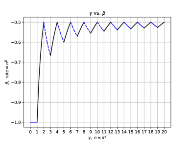
(a) Multiple descent behavior

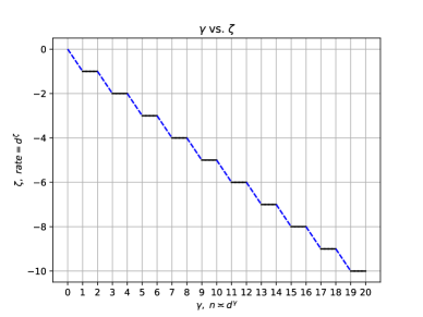
(b) Periodic plateau behavior

Figure 1: A graphical representation of the minimax optimal rate of the excess risk of kernel regression with inner product kernels obtained from Theorem 4.2, and Theorem 4.3. The solid black line represents the upper bound that matches the minimax lower bound up to a constant factor. The dashed blue line indicates that, for any $\epsilon>0$, the ratio between the upper and lower bounds differs by at most $n^{-\epsilon}$.

1.3 Notations

For two sequences $\{f(s)\}_{s\in\mathbb{N}}$ and $\{g(s)\}_{s\in\mathbb{N}}$, we use the notation $f(s)\asymp g(s)$, meaning that there are absolute constants $c,C\in(0,\infty)$, such that $c|f(s)|\leq|g(s)|\leq C|f(s)|$ for all $s\in\mathbb{N}$. For a real number $x\in\mathbb{R}$, denote by $\lceil x\rceil$ the smallest integer that is greater or equal to $x$ and by $\lfloor x\rfloor$ the greatest integer that is less or equal to $x$. For $\boldsymbol{v}\in\mathbb{R}^{d}$, denote by $\boldsymbol{v}_{(j)}$ the $j$-th component of $\boldsymbol{v}$ and denote the $\ell_{2}$ norm and supreme norm of $\boldsymbol{v}$ by $\|\boldsymbol{v}\|_{2}=(\sum_{j\in[d]}\boldsymbol{v}_{(j)}^{2})^{1/2}$ and $\|\boldsymbol{v}\|_{\infty}=\max_{j\in[d]}|\boldsymbol{v}_{(j)}|$ respectively. For a matrix $\boldsymbol{A}\in\mathbb{R}^{m\times n}$, denote by $a_{ij}$ the $(i,j)$-th component of $\boldsymbol{A}$ and denote the operator norm and the Frobenius norm of $\boldsymbol{A}$ by $\|\boldsymbol{A}\|_{\mathrm{op}}=\sup_{\boldsymbol{v}\in\mathbb{R}^{n}}\|\boldsymbol{A}\boldsymbol{v}\|_{2}/\|\boldsymbol{v}\|_{2}$ and $\|\boldsymbol{A}\|_{\mathrm{F}}=(\sum_{i\in[m],j\in[n]}a_{ij}^{2})^{1/2}$ respectively. Denote the $j$-th largest eigenvalues of the matrix $\boldsymbol{A}$ by $\lambda_{j}(\boldsymbol{A})$. For any symmetric matrix $\boldsymbol{A}$, define $\boldsymbol{A}^{2}=\boldsymbol{A}\boldsymbol{A}^{\tau}$. For a set $A$, denote by $|A|$ the number of elements $A$ contains. Let $\tau$ be a positive measure on $\mathcal{X}$. We define the space $L^{2}(\mathcal{X},\tau)=\{f:\mathcal{X}\to\mathbb{R}:\int_{\mathcal{X}}|f(\boldsymbol{x})|^{2}\mathrm{d}\tau<\infty\}$. The sphere $\mathbb{S}^{d}\subset\mathbb{R}^{d+1}$ is defined as $\mathbb{S}^{d}=\left\{(x_{1},\cdots,x_{d+1})^{\tau}\mid\sum_{i}x_{i}^{2}=1\right\}$. For any $k>0$, define $k\mathbb{S}^{d}=\left\{(x_{1},\cdots,x_{d+1})^{\tau}\mid\sum_{i}x_{i}^{2}=k^{2}\right\}$. For any positive integer $n$, denote by $\boldsymbol{I}_{n}$ the identity matrix of size $n$, denote $\mathbf{1}_{n}=(1,\cdots,1)^{\tau}\in\mathbb{R}^{n}$.

2 Bounds for large dimensional kernel regression

Traditional technical tools for kernel regression are developed implicitly under the assumption that the dimension $d$ of the domain $\mathcal{X}$ is fixed or bounded. The recent successes of neural networks in high dimensional data urge us to investigate the convergence rate of the excess risk of the NTK regression for data with large $d$.

Suppose that we have observed $n$ i.i.d. samples $(X_{i},Y_{i}),i\in[n]$ from the model:

$$y=f_{\star}(\boldsymbol{x})+\epsilon,$$ (2)

where $X_{i}$’s are sampled from $\rho_{\mathcal{X}}$, $\rho_{\mathcal{X}}$ is the marginal distribution on $\mathcal{X}\subset\mathbb{R}^{d+1}$, $f_{\star}$ is some function defined on a compact set $\mathcal{X}$, and $\epsilon\sim\mathcal{N}(0,\sigma^{2})$ for some fixed $\sigma>0$. Denote the $n\times 1$ data vector of ${Y_{i}}$’s and the $n\times d$ data matrix of $X_{i}$’s by $\boldsymbol{y}$ and $\boldsymbol{X}$ respectively.

Let us make the following assumptions on the kernel $K$ and the candidate function class $\mathcal{B}$ throughout this paper.

Assumption 1.

Suppose that $K$ is a continuous positive definite kernel function defined on $\mathcal{X}\subset\mathbb{R}^{d}$ satisfying $\max_{x\in\mathcal{X}}K(x,x)\leq 1$.

Assumption 2.

Let us consider a following family of candidate functions,

$$\mathcal{B}=\left\{f_{\star}\in\mathcal{H}~{}\bigg{|}~{}\|f_{\star}\|_{\mathcal{H}}\leq 1\right\},$$ (3)

where $\mathcal{H}$ is the RKHS associated with the kernel $K$.

Remark 2.1.

The Assumption 1 holds for a large class of kernels ( e.g. , the spherical NTK, Gaussian kernel, Laplace kernel, etc.). The Assumption 2 is merely a compact condition that is quite common and necessary regardless of the dimension $d$. Both of these two assumptions are commonly assumed in the literature on kernel methods [14, 15, 62] when the dimension $d$ of the domain is fixed or bounded.

Given a positive definite kernel function $K$ and a positive measure $\rho_{\mathcal{X}}$ on $\mathcal{X}$, the integral operator $T_{K}$ defined by

$$T_{K}(f)(x)=\int K(x,y)f(y)~{}\mathsf{d}\rho_{\mathcal{X}}(y)$$

is a self-adjoint compact operator. The celebrated Mercer’s decomposition theorem further assures that

$$K(x,y)=\sum_{j}\lambda_{j}\phi_{j}(x)\phi_{j}(y),$$ (4)

where $\{\lambda_{j},j=1,2,...\}$ and ortho-normal eigen-functions $\{\phi_{j}(x),j=1,2,...\}$ are the non-increasing ordered eigenvalues and corresponding eigen-functions of $T_{K}$. After a little bit of abuse of notations, we may call $\{\lambda_{j},j=1,2,...\}$ and $\{\phi_{j}(x),j=1,2,...\}$ the eigenvalues and eigenvectors(or eigen-functions) of the kernel function $K$ as well.

We then introduce the (population and empirical) Mendelson complexity, the key quantities in determining the minimax rate of regression over $\mathcal{B}$.

Definition 2.2 (Mendelson complexity).

Suppose that $K$ is a kernel function satisfying the Assumption 1, we then introduce:

• (Population Mendelson complexity) Let $\lambda_{i}$’s be the eigenvalues of $K$ given in (4) and $\mathcal{R}_{K}(\varepsilon):=\left[\frac{1}{n}\sum_{j=1}^{\infty}\min\left\{\lambda_{j},\varepsilon^{2}\right\}\right]^{1/2}$. The population Mendelson complexity is given by

  $${\varepsilon}_{n}:=\arg\min_{\varepsilon}\left\{{\mathcal{R}}_{{K}}(\varepsilon)\leq\varepsilon^{2}/(2e\sigma)\right\}.$$ (5)

• (Empirical Mendelson complexity) Let $\widehat{\lambda}_{i}$’s be the eigenvalues of $\frac{1}{n}K(\boldsymbol{X},\boldsymbol{X})$ and $\widehat{R}_{K}(\varepsilon)=\left[\frac{1}{n}\sum_{j=1}^{n}\min\{\widehat{\lambda}_{j},\varepsilon^{2}\}\right]^{1/2}$. The empirical Mendelson complexity is given by

  $$\widehat{\varepsilon}_{n}:=\arg\min_{\varepsilon}\left\{\widehat{\mathcal{R}}_{{K}}(\varepsilon)\leq\varepsilon^{2}/(2e\sigma)\right\}.$$ (6)

Upper bound of the excess risk of kernel regression.  The Mendelson complexity is closely related to the upper bound of the excess risk of kernel regression. More precisely, suppose that $f_{\star}\in\mathcal{H}$, a reproducible kernel Hilbert space (RKHS) [22, 40, 68] associated with a positive definite kernel function $K(\cdot,\cdot)$ defined on $\mathcal{X}$. The gradient flow of the loss function $\mathcal{L}=\frac{1}{2n}\sum_{j}(y_{j}-f(X_{j}))^{2}$ induced a gradient flow in $\mathcal{H}$ which is given by

$$\dot{f}_{t}(\boldsymbol{x})=-\frac{1}{n}K(\boldsymbol{x},\boldsymbol{X})(f_{t}(\boldsymbol{X})-\boldsymbol{y}),$$ (7)

where $\boldsymbol{X}=(X_{1},\cdots,X_{n})$, $\boldsymbol{y}=(Y_{1},\cdots,Y_{n})^{\tau}$. If we further assume that ${f}_{0}(\boldsymbol{x})=0$, then we have

$$f_{t}(\boldsymbol{x})=K(\boldsymbol{x},\boldsymbol{X})K(\boldsymbol{X},\boldsymbol{X})^{-1}(\boldsymbol{I}_{n}-e^{-\frac{1}{n}K(\boldsymbol{X},\boldsymbol{X})t})\boldsymbol{y}.$$ (8)

This $f_{t}(\boldsymbol{x})$ is referred to as the estimator given by kernel regression stopped at time $t$.

Theorem 2.3 (Upper bound).

Suppose that Assumptions  1 and 2 hold. Let $f_{\widehat{T}}$ be the function defined in (8) where $\widehat{T}=1/\widehat{\varepsilon}_{n}^{2}$. Suppose for any absolute constant $C$, there exists a constant $\mathfrak{C}$ only depending on $c_{1}$, $c_{2}$ and $\gamma$ (where $c_{1},c_{2}$ and $\gamma$ are introduced in the asymptotic framework of large dimensional data (12)), such that for any $n\geq\mathfrak{C}$, we have $n\varepsilon_{n}^{2}\geq C$. Then there exist absolute constants $C_{1}$, $C_{2}$, and $C_{3}$, and a constant $\mathfrak{C}_{0}$ only depending on $c_{1},c_{2}$, and $\gamma$, such that for any $n\geq\mathfrak{C}_{0}$, we have

$$\left\|{f}_{\widehat{T}}-f_{\star}\right\|_{L^{2}}^{2}\leq C_{1}\varepsilon_{n}^{2},$$ (9)

with probability at least $1-C_{2}\exp\left\{-C_{3}n\varepsilon_{n}^{2}\right\}$.

Similar results have been claimed in [62] for fixed $d$ ( see e.g., the Theorem 2 of [62]), the contributions here is that we demonstrate that the constants $C_{1}$, $C_{2}$, and $C_{3}$ are absolute constants. Thus, we could apply it to the large-dimensional scenario.

Remark 2.4.

Since $\varepsilon_{n}$ should be much slower than the typical parametric rate $n^{-1/2}$ [18, 35], previous works have commonly assumed the existence of constants $\mathfrak{C}$ and $C$, such that for any $n\geq\mathfrak{C}$, we have $n\varepsilon_{n}^{2}\geq C$ (e.g., [62]). However, these works implicitly assumed that $d$ is bounded and $\{\lambda_{j}\}$ are polynomially decayed and ignored the dependence of the constant $\mathfrak{C}$ on $\{\lambda_{j}\}$ and $d$. Theorem 2.3 explicitly requires that $\mathfrak{C}$ only depends on $c_{1},c_{2}$, and $\gamma$.

Lower bound of the excess risk of kernel regression. Suppose that $(\mathcal{Z},d)$ is a topological space with a compatible loss function $d$, which are mappings from $\mathcal{Z}\times\mathcal{Z}$ to $\mathbb{R}_{\geq 0}$ with $d(f,f)=0$ and $d(f,f^{\prime})>0$ for $f\neq f^{\prime}$. We call such a loss function a distance. We introduce the packing entropy and covering entropy below:

Definition 2.5 (Packing entropy).

A finite set $N_{\varepsilon}\subset\mathcal{Z}$ is said to be an $\varepsilon$-packing set in $\mathcal{Z}$ with separation $\varepsilon>0$, if for any $f,f^{\prime}\in N_{\varepsilon},f\neq f^{\prime}$, we have $d\left(f,f^{\prime}\right)>\varepsilon$. The logarithm of the maximum cardinality of $\varepsilon$-packing set is called the $\varepsilon$-packing entropy or Kolmogorov capacity of $\mathcal{Z}$ with distance $d$ and is denoted by $M_{d}(\varepsilon,\mathcal{Z})$.

Definition 2.6 (Covering entropy).

A set $G_{\varepsilon}\subset\mathcal{Z}$ is said to be an $\varepsilon$-net for $\mathcal{Z}$ if for any $\tilde{f}\in\mathcal{Z}$, there exists an $f_{0}\in G_{\varepsilon}$ such that $d(\tilde{f},f_{0})\leq\varepsilon$. The logarithm of the minimum cardinality of $\varepsilon$-net is called the $\varepsilon$-covering entropy of $\mathcal{Z}$ and is denoted by $V_{d}(\varepsilon,\mathcal{Z})$.

Let $M_{2}(\varepsilon,\mathcal{B})$ be the $\varepsilon$-packing entropy of $(\mathcal{B},d^{2}=\|\cdot\|_{L^{2}}^{2})$ and $V_{2}(\varepsilon,\mathcal{B})$ be the $\varepsilon$-covering entropy of $(\mathcal{B},d^{2}=\|\cdot\|_{L^{2}}^{2})$. It is easy to verify that $M_{2}(2\varepsilon,\mathcal{B})\leq V_{2}(\varepsilon,\mathcal{B})\leq M_{2}(\varepsilon,\mathcal{B})$ ( see, e.g., Lemma A.7 ). If we further introduce

$$\mathcal{D}=\left\{\rho_{f}~{}\bigg{|}~{}\mbox{ joint distribution of $(y,x$) where }x\sim\rho_{\mathcal{X}},y=f(x)+\epsilon,\epsilon\sim N(0,\sigma^{2}),f\in\mathcal{B}\right\},$$

and let $V_{K}(\varepsilon,\mathcal{D})$ be the $\varepsilon$-covering entropy of $(\mathcal{D},d^{2}=\text{ KL divergence })$. Then it is easy to verify that $V_{2}(\varepsilon,\mathcal{B})=V_{K}({\varepsilon}/{(\sqrt{2}\sigma)},\mathcal{D})$ ( see, e.g., Lemma A.8 ).

The following minimax lower bound is introduced in [79].

Proposition 2.7 (Theorem 1 and Corollary 1 in [79]).

Let $\bar{\varepsilon}_{n}$ and $\underline{\varepsilon}_{n}$ be given by $n\bar{\varepsilon}_{n}^{2}=V_{K}(\bar{\varepsilon}_{n},\mathcal{\mathcal{D}})$ and $M_{2}(\underline{\varepsilon}_{n},\mathcal{B})=4n\bar{\varepsilon}_{n}^{2}+2\log 2$. Suppose further that $M_{2}(\varepsilon,\mathcal{B})\geq 2\log 2$ for sufficiently small $\varepsilon$. Then we have the following statements.

• For sufficiently large $n$, we have $\underline{\varepsilon}_{n}<\infty$ and the minimax risk for estimating $f_{\star}\in\mathcal{B}$ satisfies

  $$\min_{\hat{f}}\max_{f_{\star}\in\mathcal{B}}\mathbb{E}_{(\mathbb{X},\mathbb{y})\sim\rho_{f_{\star}}^{\otimes n}}\left\|\hat{f}-f_{\star}\right\|_{L^{2}}^{2}\geq(1/8)\underline{\varepsilon}_{n}^{2};$$ (10)

• If the richness condition $\liminf_{\varepsilon\rightarrow 0}M_{2}(\alpha\varepsilon,\mathcal{B})/M_{2}(\varepsilon,\mathcal{B})=1+\delta$ holds for some $0<\alpha<1$ and some $\delta>0$, then we have

  $$\mathfrak{c}_{1}\bar{\varepsilon}_{n}^{2}\leq(1/8)\underline{\varepsilon}_{n}^{2}\leq\min_{\hat{f}}\max_{f_{\star}\in\mathcal{B}}\mathbb{E}_{(\mathbb{X},\mathbb{y})\sim\rho_{f_{\star}}^{\otimes n}}\left\|\hat{f}-f_{\star}\right\|_{L^{2}}^{2}\leq\mathfrak{c}_{2}\bar{\varepsilon}_{n}^{2},$$ (11)

  where $\mathfrak{c}_{1}$ and $\mathfrak{c}_{2}$ are constants only depending on $\alpha$ and $\delta$.

If the richness condition holds, [79] has shown that $\underline{\varepsilon}_{n}\geq 8\mathfrak{c}_{1}\bar{\varepsilon}_{n}$ and demonstrated that $\bar{\varepsilon}_{n}^{2}$ can be served as a minimax lower bound for several function classes. The constant $\mathfrak{c}_{1}$ depends on $\delta$ and $\alpha$ will be very small provided that $\delta$ is small enough ( referred to Lemma 4 in [79]). Unfortunately, if one plans to apply the Proposition 2.7 into the RKHS with large $d$, we have the following proposition showing that for the RKHS associated with NTK, $\delta$ can be arbitrarily small when $d$ is large:

Proposition 2.8.

Let $\mathcal{B}=\{f_{\star}\in\mathcal{H}^{\mathtt{NT}}~{}|~{}\|f_{\star}\|_{\mathcal{H}^{\mathtt{NT}}}\leq 1\}$, where $K^{\mathtt{NT}}$ is defined by (116) and $\mathcal{H}^{\mathtt{NT}}$ is the RKHS associated with $K^{\mathtt{NT}}$. For any $0<\alpha<1$ and any $\delta>0$, there exists a sequence $\{\tilde{\varepsilon}_{d}\}_{d=1}^{\infty}$, such that $\liminf_{d\rightarrow\infty}\tilde{\varepsilon}_{d}=0$, and we have

$$\liminf_{d\rightarrow\infty}\frac{M_{2}(\alpha\tilde{\varepsilon}_{d},\mathcal{B})}{M_{2}(\tilde{\varepsilon}_{d},\mathcal{B})}\leq 1+\delta.$$

The Proposition 2.8 reveals an essential difficulty in determining the minimax lower bound of kernel regression with large dimensional data: when $d$ is very large, the lower bound in Proposition 2.7 may become vague. To avoid potential confusion, we specify the following large dimensional scenario for kernel regression where we perform our analysis: suppose that there exist three positive constants $c_{1}$, $c_{2}$ and $\gamma$, such that

$$c_{1}d^{\gamma}\leq n\leq c_{2}d^{\gamma},$$ (12)

and we often assume that $d$ is sufficiently large. The following theorem provides a minimax lower bound of kernel regression in large dimensions.

Theorem 2.9 (Minimax lower bound).

Let $\bar{\varepsilon}_{n}$ be given by $n\bar{\varepsilon}_{n}^{2}=V_{K}(\bar{\varepsilon}_{n},\mathcal{D})$. Assume that there exists a constant $\mathfrak{C}$ only depending on $c_{1},c_{2}$ and $\gamma$, such that for any $n\geq\mathfrak{C}$, we have $n\bar{\varepsilon}_{n}^{2}\geq 2\log 2$. Then for any constants $\mathfrak{c}_{1}\leq 1/5$ and $\mathfrak{c}_{2}>0$ only depending on $c_{1},c_{2}$ and $\gamma$, such that the inequality

$$V_{K}(\bar{\varepsilon}_{n},\mathcal{\mathcal{D}})\leq\mathfrak{c}_{1}V_{2}(\mathfrak{c}_{2}\bar{\varepsilon}_{n},\mathcal{B})$$ (13)

holds for any $n\geq\mathfrak{C}$, we have

$$\min_{\hat{f}}\max_{f_{\star}\in\mathcal{B}}\mathbb{E}_{(\mathbb{X},\mathbb{y})\sim\rho_{f_{\star}}^{\otimes n}}\left\|\hat{f}-f_{\star}\right\|_{L^{2}}^{2}\geq\frac{1}{2}\left(\frac{\mathfrak{c}_{2}}{12}\right)^{2}\bar{\varepsilon}_{n}^{2},$$ (14)

where $\rho_{f_{\star}}$ is the joint-p.d.f. of $x,y$ given by (2) with $f=f_{\star}$.

Remark 2.10.

When the richness condition holds for some constants $\delta>0$ and $0<\alpha<1$, let $N$ be the smallest integer satisfying $(1+\delta)^{N}>5$. One can show that (13) holds for $\mathfrak{c}_{1}=1/5$ and $\mathfrak{c}_{2}=(1+\delta)^{N}\sigma/\sqrt{2}$ (see, e.g., Proposition A.9). In other words, the scope where the Theorem 2.9 can be applied is larger than the Proposition 2.7.

3 Optimality of kernel regression with inner product kernels in large dimensions for $\gamma=2,4,6,\cdots$

In this section, as a warm-up, we will show that the optimal rate of kernel regression with respect to the inner product kernel is $n^{-1/2}$ when $n\propto d^{\gamma},\gamma=2,4,6,\cdots.$

An inner product kernel is a kernel function $K^{in}$ defined on $\mathbb{S}^{d}$ such that there exists a function $\Phi:[-1,1]\to\mathbb{R}$ independent of $d$ satisfying that for any $\boldsymbol{x},\boldsymbol{x}^{\prime}\in\mathbb{S}^{d}$, we have $K^{\mathtt{in}}(\boldsymbol{x},\boldsymbol{x}^{\prime})=\Phi(\left\langle\boldsymbol{x},\boldsymbol{x}^{\prime}\right\rangle)$. If we further assume that the marginal distribution $\rho_{\mathcal{X}}$ is the uniform distribution on $\mathcal{X}=\mathbb{S}^{d}$, then the Mercer’s decomposition for ${K}^{\mathtt{in}}$ is given by

$${K}^{\mathtt{in}}(\boldsymbol{x},\boldsymbol{x}^{\prime})=\sum_{k=0}^{\infty}\mu_{k}\sum_{j=1}^{N(d,k)}Y_{k,j}(\boldsymbol{x})Y_{k,j}\left(\boldsymbol{x}^{\prime}\right),$$ (15)

where $Y_{k,j}$ for $j=1,\cdots,N(d,k)$ forms an orthonormal basis of the spherical harmonic polynomials of degree $k$ and $\mu_{k}$’s are the eigenvalues of $K^{\mathtt{in}}$ with multiplicity $N(d,k)=\frac{2k+d-1}{k}\cdot\frac{(k+d-2)!}{(d-1)!(k-1)!}$ ( please refer to Appendix D.1 for more details).

To avoid unnecessary notation, let us make the following assumption on the inner kernel $K^{in}$.

Assumption 3.

The coefficients $\{a_{j},j=0,1,2,...\}$ appeared in the Taylor’s expansion $\Phi(t)=\sum_{j=0}^{\infty}a_{j}t^{j}$ are positive.

The purpose of this assumption is to keep the main results and proofs clean. One can easily extend the current results without this assumption (e.g., in Section 5, we presented the results for NTK where the Assumption  3 is violated.). With this assumption, we have the following lemma which is borrowed from [30].

Lemma 3.1.

Suppose that Assumptions  1 and 3 hold. Suppose that $p\geq 0$ is any integer. There exist positive constants $\mathfrak{C}_{1}$ and $\mathfrak{C}_{2}$ only depending on $p$ and $\{a_{j}\}_{j\leq p+1}$, such that for any $d\geq\mathfrak{C}$, a sufficiently large constant only depending on $p$, we have

$${\mathfrak{C}_{1}}{d^{-k}} \leq\mu_{k}\leq{\mathfrak{C}_{2}}{d^{-k}}\quad k=0,1,2,\cdots,p,p+1.$$ (16)

Thanks to Lemma 3.1, we can now use Theorem 2.3 to provide an upper bound on the excess risk of kernel regression with the inner product kernel $K^{\mathtt{in}}$ in large dimensions.

Theorem 3.2 (Upper bound).

Suppose that $\mathcal{H}^{\mathtt{in}}$ is an RKHS associated with $K^{\mathtt{in}}$ defined on $\mathbb{S}^{d}$. Let $f_{\widehat{T}}^{\mathtt{in}}$ be the function defined in (8) where $\widehat{T}=\widehat{\varepsilon}_{n}^{-2}$ and $K=K^{\mathtt{in}}$. Suppose further that Assumptions  1,  2, and  3 hold with $\mathcal{H}=\mathcal{H}^{\mathtt{in}}$. Then, there exist constants $\mathfrak{C}_{i}$, $i=1,2,3$ only depending on ${\gamma}$, such that for any $d\geq\mathfrak{C}$, a sufficiently large constant only depending on $c_{1}$, $c_{2}$, and ${\gamma}$ defined in (12), we have

$$\left\|{f}_{\widehat{T}}^{\mathtt{in}}-f_{\star}\right\|_{L^{2}}^{2}\leq\mathfrak{C}_{1}n^{-\frac{1}{2}},$$ (17)

with probability at least $1-\mathfrak{C}_{2}\exp\left\{-\mathfrak{C}_{3}n^{1/2}\right\}$.

The following property of the eigenvalues $\{\mu_{k}\}_{k\geq 0}$ is crucial to determining the minimax lower bound of large-dimensional kernel regression.

Lemma 3.3.

Suppose that Assumptions  1 and 3 hold. Fixed an integer $p\geq 0$. Then, for any $d\geq\mathfrak{C}$, a sufficiently large constant only depending on $p$, we have

$$\mu_{j}\leq\frac{\mathfrak{C}_{2}}{\mathfrak{C}_{1}}d^{-1}\mu_{p},\quad j=p+1,p+2,\cdots,$$

where $\mathfrak{C}_{1}$ and $\mathfrak{C}_{2}$ are constants only depending on $p$ and $\{a_{j}\}_{j\leq p+2}$ given in Lemma 3.1.

We then use Theorem 2.9 to show that kernel regression with $K^{\mathtt{in}}$ achieves the optimal rate under specific asymptotic frameworks.

Theorem 3.4 (Minimax lower bound).

Let ${\gamma}\in\{2,4,6,\cdots\}$ be a fixed integer. There exist constants $\mathfrak{C}$ and $\mathfrak{C}_{1}$ only depending on $c_{1}$, $c_{2}$, and ${\gamma}$, such that for any $d\geq\mathfrak{C}$, we have

$$\min_{\hat{f}}\max_{f_{\star}\in\mathcal{B}}\mathbb{E}_{(\mathbb{X},\mathbb{y})\sim\rho_{f_{\star}}^{\otimes n}}\left\|\hat{f}-f_{\star}\right\|_{L^{2}}^{2}\geq\mathfrak{C}_{1}n^{-\frac{1}{2}},$$ (18)

where $\rho_{f_{\star}}$ is the joint-p.d.f. of $x,y$ given by (2) with $f=f_{\star}$, $\mathcal{B}=\{f_{\star}\in\mathcal{H}^{\mathtt{in}}~{}\mid~{}\|f_{\star}\|_{\mathcal{H}^{\mathtt{in}}}\leq 1\}$.

Notice that Theorem 3.2 and Theorem 3.4 only show the optimality of kernel regression with $K^{\mathtt{in}}$ when $n\asymp d^{\gamma}$ for $\gamma=2,4,6,\cdots$. In the next section, we will modify the existing tools for bounding the excess risk of kernel regression with $K^{\mathtt{in}}$, and show the optimality of kernel regression with $K^{\mathtt{in}}$ when $n\asymp d^{\gamma}$ for any $\gamma>0$.

4 Optimality of kernel regression in large dimensions for all $\gamma>0$

We have shown that in the large dimensional setting where $n\asymp d^{\gamma},\gamma=2,4,6,\cdots$, the optimal rate of the kernel regression with $K^{\mathtt{in}}$ for large dimensional data is $n^{-1/2}$.

However, when $\gamma\neq 2,4,6,\cdots$, Theorem 2.9 can not be applied to large-dimensional kernel regression. For example, when $\gamma\in(2p,2p+1]$ for some integer $p\geq 0$, we have $\mathfrak{C}_{4}d^{p-\gamma}\log(d)\leq\bar{\varepsilon}_{n}\leq\mathfrak{C}_{3}d^{p-\gamma}\log(d)\ll n^{-1/2}$, where $\mathfrak{C}_{3}$ and $\mathfrak{C}_{4}$ are constants only depending on $\gamma$, $c_{1}$, and $c_{2}$ (see e.g., Remark C.2). However, the inequality (13) does not hold (see, e.g., Lemma C.1). Furthermore, the upper bound $n^{-1/2}$ provided by Theorem 2.3 is no longer matching the metric entropy $\bar{\varepsilon}_{n}^{2}$.

The main focus of this section is trying to determine the optimal rate for all the $\gamma>0$. To construct a minimax lower bound for regression over the unit ball $\mathcal{B}\subset\mathcal{H}^{\mathtt{in}}$, we need the following modification of Proposition 2.7.

Lemma 4.1.

Let $\mathfrak{c}\in(0,1)$ be a constant only depending on $c_{1}$, $c_{2}$, and $\gamma$. For any $0<\tilde{\varepsilon}_{1},\tilde{\varepsilon}_{2}<\infty$ only depending on $n$, $d$, $\{\lambda_{j}\}$, $c_{1}$, $c_{2}$, and $\gamma$ and satisfying

$$\frac{V_{K}(\tilde{\varepsilon}_{2},\mathcal{D})+n\tilde{\varepsilon}_{2}^{2}+\log(2)}{V_{2}(\tilde{\varepsilon}_{1},\mathcal{B})}\leq\mathfrak{c},$$ (19)

we have

$$\min_{\hat{f}}\max_{f_{\star}\in\mathcal{B}}\mathbb{E}_{(\mathbb{X},\mathbb{y})\sim\rho_{f_{\star}}^{\otimes n}}\left\|\hat{f}-f_{\star}\right\|_{L^{2}}^{2}\geq\frac{1-\mathfrak{c}}{4}\tilde{\varepsilon}_{1}^{2},$$ (20)

where $\rho_{f_{\star}}$ is the joint-p.d.f. of $x,y$ given by (2) with $f=f_{\star}$.

We then have the following minimax lower bounds, which greatly extend the results given in Theorem 3.4:

Theorem 4.2.

Let $\rho_{f_{\star}}$ be the joint-p.d.f. of $x,y$ given by (2) with $f_{\star}\in\mathcal{B}=\{f\in\mathcal{H}^{\mathtt{in}}~{}\mid~{}\|f\|_{\mathcal{H}^{\mathtt{in}}}\leq 1\}$. Let $\gamma>0$ be a fixed real number and $p=\lfloor\gamma/2\rfloor$. Then we have the following statements.

• If $\gamma\in\{2,4,6,\cdots\}$, then, there exist constants $\mathfrak{C}_{1}>0$ and $\mathfrak{C}$ only depending on $c_{1}$, $c_{2}$, and $\gamma$, such that for any $d\geq\mathfrak{C}$, we have:

  $$\min_{\hat{f}}\max_{f_{\star}\in\mathcal{B}}\mathbb{E}_{(\mathbb{X},\mathbb{y})\sim\rho_{f_{\star}}^{\otimes n}}\left\|\hat{f}-f_{\star}\right\|_{L^{2}}^{2}\geq\mathfrak{C}_{1}n^{-\frac{1}{2}};$$ (21)

• If $\gamma\in\bigcup_{j=0}^{\infty}(2j,2j+1]$, then, for any $\epsilon>0$, there exist constants $\mathfrak{C}_{1}>0$ and $\mathfrak{C}$ only depending on $c_{1}$, $c_{2}$, $\gamma$, and $\epsilon$, such that for any $d\geq\mathfrak{C}$, we have:

  $$\min_{\hat{f}}\max_{f_{\star}\in\mathcal{B}}\mathbb{E}_{(\mathbb{X},\mathbb{y})\sim\rho_{f_{\star}}^{\otimes n}}\left\|\hat{f}-f_{\star}\right\|_{L^{2}}^{2}\geq\mathfrak{C}_{1}n^{-\left(\frac{\gamma-p}{\gamma}+\epsilon\right)};$$ (22)

• If $\gamma\in\bigcup_{j=0}^{\infty}(2j+1,2j+2)$, then, there exist constants $\mathfrak{C}_{1}>0$ and $\mathfrak{C}$ only depending on $c_{1}$, $c_{2}$, and $\gamma$, such that for any $d\geq\mathfrak{C}$, we have:

  $$\min_{\hat{f}}\max_{f_{\star}\in\mathcal{B}}\mathbb{E}_{(\mathbb{X},\mathbb{y})\sim\rho_{f_{\star}}^{\otimes n}}\left\|\hat{f}-f_{\star}\right\|_{L^{2}}^{2}\geq\mathfrak{C}_{1}n^{-\frac{p+1}{\gamma}}.$$ (23)

Since the upper bound provided by the Mendelson complexity is no longer a tight upper bound, we have to improve the claims in Theorem 3.2. Fortunately, thanks to a nontrivial technical observation, we then present new upper bounds on the excess risk of kernel regression in large dimensions which (nearly) match the minimax lower bounds given in Theorem 4.2.

Theorem 4.3.

Suppose that $\mathcal{H}^{\mathtt{in}}$ is an RKHS associated with $K^{\mathtt{in}}$ defined on $\mathbb{S}^{d}$. Let $f_{\widehat{T}}^{\mathtt{in}}$ be the function defined in (8) where $\widehat{T}=\widehat{\varepsilon}_{n}^{-2}$ and $K=K^{\mathtt{in}}$. Suppose further that Assumptions  1,  2, and  3 hold with $\mathcal{H}=\mathcal{H}^{\mathtt{in}}$. Let $\gamma>0$ be a fixed real number and $p=\lfloor\gamma/2\rfloor$. Then, we have the following statements:

• If $\gamma\in\{2,4,6,\cdots\}$, then, there exist constants $\mathfrak{C}$ and $\mathfrak{C}_{i}$, where $i=1,2,3$, only depending on $\gamma$, $c_{1}$, and $c_{2}$, such that for any $d\geq\mathfrak{C}$, we have

  $$\left\|{f}_{\widehat{T}}^{\mathtt{in}}-f_{\star}\right\|_{L^{2}}^{2}\leq\mathfrak{C}_{1}n^{-\frac{1}{2}}$$ (24)

  holds with probability at least $1-\mathfrak{C}_{2}\exp\{-\mathfrak{C}_{3}n^{1/2}\}$.

• If $\gamma\in\bigcup_{j=0}^{\infty}(2j,2j+1]$, then, for any $\delta>0$, there exist constants $\mathfrak{C}$ and $\mathfrak{C}_{i}$, where $i=1,2,3$, only depending on $\gamma$, $\delta$, $c_{1}$, and $c_{2}$, such that for any $d\geq\mathfrak{C}$, we have

  $$\left\|{f}_{\widehat{T}}^{\mathtt{in}}-f_{\star}\right\|_{L^{2}}^{2}\leq\mathfrak{C}_{1}n^{-\frac{\gamma-p}{\gamma}}\log(n)$$ (25)

  holds with probability at least $1-\delta-\mathfrak{C}_{2}\exp\{-\mathfrak{C}_{3}n^{p/\gamma}\log(n)\}$.

• If $\gamma\in\bigcup_{j=0}^{\infty}(2j+1,2j+2)$, then, for any $\delta>0$, there exist constants $\mathfrak{C}$ and $\mathfrak{C}_{i}$, where $i=1,2,3$, only depending on $\gamma$, $\delta$, $c_{1}$, and $c_{2}$, such that for any $d\geq\mathfrak{C}$, we have

  $$\left\|{f}_{\widehat{T}}^{\mathtt{in}}-f_{\star}\right\|_{L^{2}}^{2}\leq\mathfrak{C}_{1}n^{-\frac{p+1}{\gamma}}$$ (26)

  holds with probability at least $1-\delta-\mathfrak{C}_{2}\exp\{-\mathfrak{C}_{3}n^{1-(p+1)/\gamma}\}$.

Figure 1 illustrates the results obtained by Theorem 4.2 and Theorem 4.3. From these figures, we observe some interesting phenomena.

Multiple descent behavior

The curve in figure 1 (a) shows how the convergence rate (in terms of the sample size $n$) of the optimal excess risk of kernel regression fluctuates as $\gamma>0$ grows. We find that this curve is non-monotone and exhibits the following multiple descent behavior: this curve achieves its peaks at $\gamma=2,4,6,\cdots$ and its isolated valleys at $\gamma=3,5,7,\cdots$. A similar multiple descent phenomenon has been reported in [49], where they consider the excess risk of the kernel interpolation in large-dimensional settings. Though they only provided the upper bound of the excess risk of kernel interpolation, their results and our observation strongly suggest that there might be a significant difference between kernel regression in large dimensional data and fixed dimensional data.

Figure 1 (b) provides an alternative representation of our results, and the curve in it shows how the convergence rate (in terms of the dimension $d$) of the optimal excess risk of kernel regression fluctuates as $\gamma>0$ grows. From Figure 1 (b), we can find that the curve of this convergence rate decreases when the scaling $\gamma$ (recall that we have $n=d^{\gamma}$) increases, indicating that the performance of kernel regression becomes better when the sample size $n$ grows. Moreover, from Figure 1 (b), we observe another interesting phenomenon:

Periodic plateau behavior

In Figure 1 (b), when $\gamma$ varies within certain specific ranges, $\zeta$, the vertical axis in Figure 1 (b), does not change. In other words, if we fix a large dimension $d$ and increase $\gamma$ (or equivalently, increase the sample size $n$), the optimal rate of excess risk in kernel regression stays invariant in certain ranges (e.g., $\gamma\in(1,2)\cup(3,4)\cup(5,6)\cup(7,8)\cdots$). This ‘periodic plateau behavior’ was numerically reported in Figure 5 (b) in [12]: when $\gamma$ varies within certain specific ranges, the excess risk of kernel regression decays very slowly.

Therefore, in order to improve the rate of excess risk, one has to increase the sample size above a certain threshold. For example, when $d=10$, even when the sample size $n$ ranges from ten million ($10^{7}$) to hundred million ($10^{8}$), the convergence speed of excess risk stays invariant, and is proportional to $10^{-4}$.

5 Applications in Wide Neural Network

Let us consider the square loss function

$$\mathcal{L}=\frac{1}{2n}\sum_{j=1}^{n}(Y_{j}-f^{m}_{\boldsymbol{\theta}}(X_{j}))^{2},$$ (27)

where $f^{m}_{\boldsymbol{\theta}}(\boldsymbol{x})=\sqrt{\frac{1}{m}}\sum_{r=1}^{m}\left(a_{r}\left(\left\langle\boldsymbol{w}_{r},\boldsymbol{x}\right\rangle\right)^{+}\right)$ is a two-layer ReLU neural network. Denote $\operatorname{vec}\left(\left\{a_{r},\boldsymbol{w}_{r};r\in[m]\right\}\right)\in\mathbb{R}^{m(d+2)\times 1}$, the parameters of the neural network, by $\boldsymbol{\theta}$.

The loss function $\mathcal{L}$ induced a gradient flow on $\mathcal{F}^{m}$, the space of all the two-layer neural networks with width $m$, which is given by

$$\dot{f}_{\boldsymbol{\theta}(t)}^{m}(\boldsymbol{x})=-\frac{1}{n}\nabla_{\boldsymbol{\theta}}f_{\boldsymbol{\theta}(t)}^{m}(\boldsymbol{x})\nabla_{\boldsymbol{\theta}}f_{\boldsymbol{\theta}(t)}^{m}(\boldsymbol{X})^{\mathsf{T}}(f_{\boldsymbol{\theta}(t)}^{m}(\boldsymbol{X})-\boldsymbol{y}).$$ (28)

If we introduce a time-varying kernel function $K_{\boldsymbol{\theta}(t)}^{m}(\boldsymbol{x},\boldsymbol{x}^{\prime}):=\nabla_{\boldsymbol{\theta}}f_{\boldsymbol{\theta}(t)}^{m}(\boldsymbol{x})\nabla_{\boldsymbol{\theta}}f_{\boldsymbol{\theta}(t)}^{m}(\boldsymbol{x}^{\prime})$, which is referred to as the neural network kernel (NNK) in this paper, the gradient flow on $\mathcal{F}^{m}$ can be written as

$$\dot{f}_{\boldsymbol{\theta}(t)}^{m}(\boldsymbol{x})=-\frac{1}{n}K_{\boldsymbol{\theta}(t)}^{m}(\boldsymbol{x},\boldsymbol{X})(f_{\boldsymbol{\theta}(t)}^{m}(\boldsymbol{X})-\boldsymbol{y}).$$

The celebrated work [38] observed that as $m\rightarrow\infty$, the neural network kernel $K_{\boldsymbol{\theta}(t)}^{m}(\boldsymbol{x},\boldsymbol{x}^{\prime})$ point-wisely converges to a time-invariant kernel $K^{NT}(\boldsymbol{x},\boldsymbol{x^{\prime}})$ which is now referred to as the neural tangent kernel (NTK) in literature. Thus, they considered the regressor ${f}_{t}^{\mathtt{NT}}$, which is also known as the estimator produced by the early-stopping kernel regression with NTK, given by the following gradient flow

$$\dot{f}_{t}^{\mathtt{NT}}(\boldsymbol{x}) =-\frac{1}{n}K^{\mathtt{NT}}(\boldsymbol{x},\boldsymbol{X})(f_{t}^{\mathtt{NT}}(\boldsymbol{X})-\boldsymbol{y}).$$ (29)

In the remainder of this article, we will abbreviate early-stopping kernel regression with NTK to ‘NTK regression’ where it will not cause confusion.

Suppose that $f^{\mathtt{NT}}_{0}(\boldsymbol{x})=0$. Recently, [43] demonstrated that, with the symmetric initialization such that $f^{m}_{\boldsymbol{\theta}(0)}(\boldsymbol{x})=0$ [19, 37] ( i.e., $a_{r}(0),\boldsymbol{w}_{r,j}(0)\sim\mathcal{N}(0,1)$ for $r\in[m/2]$, $j\in[d+1],a_{r+m/2}(0)=a_{r}(0)$ and $\boldsymbol{w}_{r+m/2,j}(0)=\boldsymbol{w}_{r,j}(0)$), the excess risk of an wide two-layer neural network $\mathcal{E}({f}_{\boldsymbol{\theta}(t)}^{m})$ uniformly converges to the excess risk of NTK regression $\mathcal{E}\left({f}_{t}^{\mathtt{NT}}\right)$ for any values of $d$ and $n$. The following proposition reiterates their findings.

Proposition 5.1 (Theorem 3.1 in [43]).

Suppose that $\mathcal{X}$ is a bounded subset of $\mathbb{R}^{d+1}$. If we further assumed that $f^{\mathtt{NT}}_{0}=0$ and the neural network is initialized symmetrically, then for any $\epsilon,\delta>0$, there exists $M$ such that for any $m\geq M$, the excess risk $\|{f}_{\boldsymbol{\theta}(t)}^{m}-f_{\star}\|_{L^{2}}^{2}$ uniformly converges to the excess risk $\|{f}_{t}^{\mathtt{NT}}-f_{\star}\|_{L^{2}}^{2}$ with probability at least $1-\delta$ where the randomness comes from the initialization of the networks, i.e.,

$$\sup_{t\geq 0}\left|\left\|{f}_{\boldsymbol{\theta}(t)}^{m}-f_{\star}\right\|_{L^{2}}^{2}-\left\|{f}_{t}^{\mathtt{NT}}-f_{\star}\right\|_{L^{2}}^{2}\right|\leq\epsilon.$$ (30)

Thanks to the Proposition 5.1, we can focus on the generalization ability of the kernel regression with respect to NTK in large dimensions instead of that of wide neural networks.

The following theorems provide an upper bound and a minimax lower bound on the excess risk of NTK regression in large dimensions. Since the proofs of Theorem 5.2 and Theorem 5.3 are similar to the proofs of Theorem 4.2 and Theorem 4.3, we state them without proofs.

Theorem 5.2.

Let $\rho_{f_{\star}}$ be the joint-p.d.f. of $x,y$ given by (2) with $f_{\star}\in\mathcal{B}=\{f\in\mathcal{H}^{\mathtt{NT}}~{}\mid~{}\|f\|_{\mathcal{H}^{\mathtt{NT}}}\leq 1\}$. Let $\gamma>0$ be a fixed real number and $p\geq 0$ be an integer defined in the following way:

$$p=\begin{cases}\lfloor\gamma/2\rfloor&0<\gamma<4,\\[3.0pt] 2\lfloor\gamma/4\rfloor&\gamma\geq 4.\end{cases}$$ (31)

Then we have the following statements.

• If $\gamma\in\{2\}\cup\{4,8,12,\cdots\}$, then, there exist constants $\mathfrak{C}_{1}>0$ and $\mathfrak{C}$ only depending on $c_{1}$, $c_{2}$, and $\gamma$, such that for any $d\geq\mathfrak{C}$, we have:

  $$\min_{\hat{f}}\max_{f_{\star}\in\mathcal{B}}\mathbb{E}_{(\mathbb{X},\mathbb{y})\sim\rho_{f_{\star}}^{\otimes n}}\left\|\hat{f}-f_{\star}\right\|_{L^{2}}^{2}\geq\mathfrak{C}_{1}n^{-\frac{1}{2}};$$ (32)

• If $\gamma\in(0,1]\cup(2,3]\cup\bigcup_{j=1}^{\infty}(4j,4j+2]$, then, for any $\epsilon>0$, there exist constants $\mathfrak{C}_{1}>0$ and $\mathfrak{C}$ only depending on $c_{1}$, $c_{2}$, $\gamma$, and $\epsilon$, such that for any $d\geq\mathfrak{C}$, we have:

  $$\min_{\hat{f}}\max_{f_{\star}\in\mathcal{B}}\mathbb{E}_{(\mathbb{X},\mathbb{y})\sim\rho_{f_{\star}}^{\otimes n}}\left\|\hat{f}-f_{\star}\right\|_{L^{2}}^{2}\geq\mathfrak{C}_{1}n^{-\left(\frac{\gamma-p}{\gamma}+\epsilon\right)};$$ (33)

• If $\gamma\in(1,2)\cup(3,4)\cup\bigcup_{j=1}^{\infty}(4j+2,4j+4)$, then, there exist constants $\mathfrak{C}_{1}>0$ and $\mathfrak{C}$ only depending on $c_{1}$, $c_{2}$, and $\gamma$, such that for any $d\geq\mathfrak{C}$, we have:

  $$\min_{\hat{f}}\max_{f_{\star}\in\mathcal{B}}\mathbb{E}_{(\mathbb{X},\mathbb{y})\sim\rho_{f_{\star}}^{\otimes n}}\left\|\hat{f}-f_{\star}\right\|_{L^{2}}^{2}\geq\mathfrak{C}_{1}n^{-\frac{p+1+\mathbf{1}\{p\geq 2\}}{\gamma}}.$$ (34)

Theorem 5.3.

Suppose that $\mathcal{H}^{\mathtt{NT}}$ is an RKHS associated with the neural tangent kernel $K^{\mathtt{NT}}$ defined on $\mathbb{S}^{d}$, where $K^{\mathtt{NT}}$ is defined by (116). Let $f_{\widehat{T}}^{\mathtt{NT}}$ be the function defined in (8) where $\widehat{T}=\widehat{\varepsilon}_{n}^{-2}$ and $K=K^{\mathtt{NT}}$. Suppose further that Assumption  2 holds with $\mathcal{H}=\mathcal{H}^{\mathtt{NT}}$. Let $\gamma>0$ be a fixed real number. Define the integer $p$ as in (31). Then, we have the following statements:

• If $\gamma\in\{2\}\cup\{4,8,12,\cdots\}$, then, there exist constants $\mathfrak{C}$ and $\mathfrak{C}_{i}$, where $i=1,2,3$, only depending on $\gamma$, $c_{1}$, and $c_{2}$, such that for any $d\geq\mathfrak{C}$, we have

  $$\left\|{f}_{\widehat{T}}^{\mathtt{NT}}-f_{\star}\right\|_{L^{2}}^{2}\leq\mathfrak{C}_{1}n^{-\frac{1}{2}}$$ (35)

  holds with probability at least $1-\mathfrak{C}_{2}\exp\{-\mathfrak{C}_{3}n^{1/2}\}$.

• If $\gamma\in(0,1]\cup(2,3]\cup\bigcup_{j=1}^{\infty}(4j,4j+2]$, then, for any $\delta>0$, there exist constants $\mathfrak{C}$ and $\mathfrak{C}_{i}$, where $i=1,2,3$, only depending on $\gamma$, $\delta$, $c_{1}$, and $c_{2}$, such that for any $d\geq\mathfrak{C}$, we have

  $$\left\|{f}_{\widehat{T}}^{\mathtt{NT}}-f_{\star}\right\|_{L^{2}}^{2}\leq\mathfrak{C}_{1}n^{-\frac{\gamma-p}{\gamma}}\log(n)$$ (36)

  holds with probability at least $1-\delta-\mathfrak{C}_{2}\exp\{-\mathfrak{C}_{3}n^{p/\gamma}\log(n)\}$.

• If $\gamma\in(1,2)\cup(3,4)\cup\bigcup_{j=1}^{\infty}(4j+2,4j+4)$, then, for any $\delta>0$, there exist constants $\mathfrak{C}$ and $\mathfrak{C}_{i}$, where $i=1,2,3$, only depending on $\gamma$, $\delta$, $c_{1}$, and $c_{2}$, such that for any $d\geq\mathfrak{C}$, we have

  $$\left\|{f}_{\widehat{T}}^{\mathtt{NT}}-f_{\star}\right\|_{L^{2}}^{2}\leq\mathfrak{C}_{1}n^{-\frac{p+1+\mathbf{1}\{p\geq 2\}}{\gamma}}$$ (37)

  holds with probability at least $1-\delta-\mathfrak{C}_{2}\exp\{-\mathfrak{C}_{3}n^{1-(p+1+\mathbf{1}\{p\geq 2\})/\gamma}\}$.

Figure 2 provides a graphical illustration of Theorem 5.2 and Theorem 5.3. It is clear that the NTK regression with large dimensional data exhibits the multiple descent behavior and the periodic plateau behavior as well, though there might be a slight difference compared with those in Figure 1.

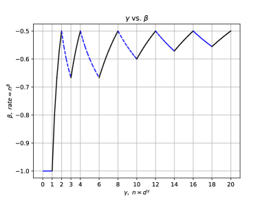
(a) Multiple descent behavior

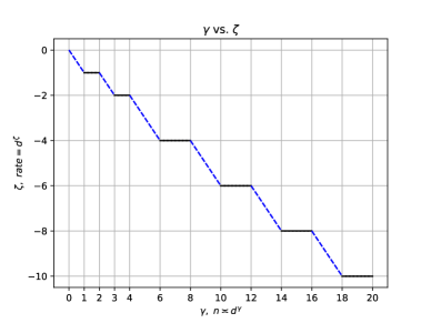
(b) Periodic plateau behavior

Figure 2: A graphical representation of the minimax optimal rate of the excess risk of NTK regression obtained from Theorem 5.2 and Theorem 5.3. The solid black line represents the upper bound that matches the minimax lower bound up to a constant factor. The dashed blue line indicates that, for any $\epsilon>0$, the ratio between the upper and lower bounds differs by at most $n^{-\epsilon}$.

6 Conclusion and Future Works

Since [38] introduced the NTK, studying the generalization performance of kernel methods has become a natural surrogate for studying the generalization performance of neural networks. In the past several years, lots of works have been done in kernel regression with fixed-dimension (e.g. [15, 46, 62, 69, 80, 81]). Though these works greatly extend our understanding of kernel regression, they also raise more natural problems for us. For example, [46] showed that fixed-dimensional kernel interpolation generalized poorly, which conflicts with the widely observed ‘benign overfitting’ phenomenon. Some researchers then speculated that in certain scenarios, the ‘benign overfitting phenomenon’ might be due to the large dimensionality of data. This urges researchers to study the kernel regression over large dimensional data (i.e., $n\asymp d^{\gamma}$ for some $\gamma>0$) ( see, e.g., [24, 30, 48, 49, 51, 64, 78]).

In this paper, we built a set of technical tools to study kernel regression in large dimensions (where the sample size $n$ was polynomially depending on the dimensionality $d$, i.e., $n\asymp d^{\gamma}$ for some $\gamma>0$). We have shown that a properly chosen early stopping rule results in a fitting function with its excess risk (generalization error) upper bounded by the Mendelson complexity $\varepsilon_{n}$ and the minimax lower bound of the generalization error is bounded below by the metric entropy $\bar{\varepsilon}_{n}$. We then examined the spherical data. Provided that $f_{\star}$ fell into the unit ball of $\mathcal{H}^{\mathtt{in}}$, the RKHS associated with an inner product kernel $K^{\mathtt{in}}$, we showed in Theorem 3.2 and Theorem 3.4 that the minimax rate of the excess risk of kernel regression with $K^{\mathtt{in}}$ is $n^{-1/2}$ when $n\asymp d^{\gamma}$ for any $\gamma=2,4,6,\cdots$. Then, in Section 4, we determined the minimax rate of kernel regression with $K^{\mathtt{in}}$ when $n\asymp d^{\gamma}$ for any $\gamma>0$. We also found some intriguing phenomena exhibited in large-dimension kernel regression, which were referred to as the ‘multiple descent behavior’ and the ‘periodic plateau behavior’.

This periodic behavior has been observed in a variety of research. For example, there are some works discussing the inconsistency of kernel methods with inner product kernels when $n\asymp d^{\gamma}$ for some non-integer $\gamma$ ( see e.g., [29, 30, 31, 55, 58]). Denote $R_{\mathrm{KR}}\left(f_{\star},\boldsymbol{X},\lambda\right)$ as the excess risk of kernel ridge regression and $\mathrm{P}_{>\ell}$ as the projection onto polynomials with degree $>\ell$. [30] showed that for any $\varepsilon>0$ and any regularization parameter $0<\lambda<\lambda^{*}$ with high probability, one has

$$\left|R_{\mathrm{KR}}\left(f_{\star},\boldsymbol{X},\lambda\right)-\left\|\mathrm{P}_{>\ell}f_{\star}\right\|_{L^{2}}^{2}\right|\leq\varepsilon\left(\left\|f_{\star}\right\|_{L^{2}}^{2}+\sigma^{2}\right),$$ (38)

where $\ell=\lfloor\gamma\rfloor$ and $\lambda^{*}$ is defined as (20) in [30]. They provided a cartoon representation of their results ( we replicated it in Figure 3 (a)).

Furthermore, there is also another line of work that obtained an upper bound on the convergence rate of the excess risk of kernel interpolation [49]. With the assumption that the regression function can be expressed as $f_{\star}(x)=\langle K(x,\cdot),\rho_{\star}(\cdot)\rangle_{L^{2}}$, with $\|\rho_{\star}\|_{L^{4}}^{4}\leq C$ for some constant $C>0$, they showed that with probability at least $1-\delta-\exp\{n/d^{\ell}\}$,

$$\left\|{f}_{\infty}^{\mathtt{in}}-f_{\star}\right\|_{L^{2}}^{2}\leq\mathfrak{C}_{1}n^{-\eta(\gamma)},$$ (39)

where $\ell=\lfloor\gamma\rfloor$, and $\eta(\gamma)=\min\left\{(\ell+1)/\gamma-1,1-\ell/\gamma\right\}$. In Figure 3 (c), we plot the upper bound results in [49] for kernel interpolation, represented by the orange line. It is clear that this curve also exhibits similar periodic behavior.

The new periodic phenomena exhibited in kernel regression with large dimensional data might be an interesting research direction. Motivated by recent work in kernel regression with fixed dimensions, we believe that there might be a uniform explanation for this periodic behavior of kernel regression with respect to the inner product kernels. In particular, whether the periodic plateau behavior holds for more general classes of kernels defined on some domain other than $\mathbb{S}^{d}$ would be of great interest.

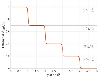
(a)

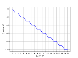
(b)

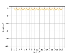
(c)

Figure 3: (a) A cartoon of the excess risk of kernel ridge regression when $f_{\star}$ is square-integrable. Borrowed from [30]. (b) The excess risk of early-stopping kernel regression when $f_{\star}\in\mathcal{H}^{\mathtt{in}}$. Obtained from Theorem 5.2 and Theorem 5.3. (c) The excess risk of kernel interpolation when $f_{\star}\in\mathcal{H}^{\mathtt{in}}$. Obtained from results in [49].

Supplement to "Optimal Rate of Kernel Regression in Large Dimensions"

Appendix A Proof of Theorems in Section 2

A.1 Proof of Theorem 2.3

The proof is divided into four lemmas below:

Lemma A.1.

Let $\widehat{\varepsilon}_{n}$ be the empirical Mendelson complexity defined in (6). There exist absolute constants $C_{2}$ and $C_{3}$ such that we have

$$\left\|f_{\widehat{T}}-f_{\star}\right\|_{n}^{2}\leq\frac{\sigma^{2}+1}{\sigma^{2}}\widehat{\varepsilon}_{n}^{2},$$ (40)

with probability at least $1-C_{2}\exp\left(-C_{3}n\widehat{\varepsilon}_{n}^{2}\right)$, where $\|g\|^{2}_{n}=\frac{1}{n}\sum_{j\leq n}g(x_{j})^{2}$, and the randomness comes from the noise term $\boldsymbol{y}-f_{\star}(\boldsymbol{X})$.

Lemma A.2.

Let $\varepsilon_{n}$ be the population Mendelson complexity defined in (5). There exist absolute constants $C_{1}$, $C_{2}$, and $C_{3}$, such that for any $M>0$, let $M\mathcal{B}:=\left\{g\in\mathcal{H}\mid\|g\|_{\mathcal{H}}\leq M\right\}$, then we have

$$\left|\|g\|_{n}^{2}-\|g\|_{L^{2}}^{2}\right|\leq\frac{1}{2}\|g\|_{L^{2}}^{2}+C_{1}{M^{2}\varepsilon_{n}^{2}}\quad\text{ for all }g\in M\mathcal{B},$$ (41)

holds with probability at least $1-C_{2}e^{-C_{3}n\varepsilon_{n}^{2}}$, where the randomness comes from $n$ samples $x_{1},\cdots,x_{n}$.

Lemma A.3.

Let $\widehat{\varepsilon}_{n}$ be the empirical Mendelson complexity defined in (6) and $\varepsilon_{n}$ be the population Mendelson complexity defined in (5). Under the same assumptions as Theorem 2.3, there exist absolute constants $C_{1}$, $C_{2}$, $C_{3}$, $C_{4}$, and a constant $\mathfrak{C}_{0}$ only depending on $c_{1}$,$c_{2}$ and $\gamma$, such that for any $n\geq\mathfrak{C}_{0}$, we have

$$C_{1}{\varepsilon}_{n}\leq\widehat{\varepsilon}_{n}\leq C_{2}{\varepsilon}_{n},$$ (42)

holds with probability at least $1-C_{3}\exp\left\{-C_{4}n\varepsilon_{n}^{2}\right\}$, where the randomness comes from $n$ samples $x_{1},\cdots,x_{n}$.

Lemma A.4.

There exists an absolute constant $C_{1}$, such that

$$\|{f}_{\widehat{T}}-f_{\star}\|_{\mathcal{H}} \leq 3,$$ (43)

holds with probability at least $1-C_{1}\exp\left\{-n(\min\{\widehat{\varepsilon}_{n},\varepsilon_{n}\})^{2}\right\}$, where the randomness comes from the noise term $\boldsymbol{y}-f_{\star}(\boldsymbol{X})$.

It is a tedious work to show that these constants are absolute constants. We defer the details of the proofs to Appendix E.2. Now let’s begin the proof of Theorem 2.3. Thanks to the Lemma A.3, we know the following three statements hold with probability at least $1-C_{2}\exp\{-C_{3}n\varepsilon_{n}^{2}\}$ for some absolute constants $C_{1}$, $C_{2}$, and $C_{3}$.

• Lemma A.1 and A.3 imply that $\|f_{\widehat{T}}-f_{\star}\|_{n}^{2}\leq\frac{\sigma^{2}+1}{\sigma^{2}}\widehat{\varepsilon}_{n}^{2}\leq C_{1}\varepsilon_{n}^{2}$.

• Lemma A.4 guarantees $\frac{1}{3}\left({f}_{\widehat{T}}-f_{\star}\right)\in\mathcal{B}$.

• Lemma A.2 then guarantees

  $$\frac{1}{2}\|{f}_{\widehat{T}}-f_{\star}\|_{L^{2}}^{2}\leq\|{f}_{\widehat{T}}-f_{\star}\|_{n}^{2}+{9C_{1}\varepsilon_{n}^{2}},$$ (44)

Conditioning on the event that both (40), (42), (43), and (44) hold. we have

$$\|f_{\widehat{T}}-f_{\star}\|^{2}_{L^{2}}{\leq}2\|{f}_{\widehat{T}}-f_{\star}\|_{n}^{2}+{C_{1}\varepsilon_{n}^{2}}\leq 3C_{1}\varepsilon_{n}^{2},$$

holds with probability at least $1-C_{2}\exp\left\{-C_{3}n\varepsilon_{n}^{2}\right\}$. $\square$

A.2 Proof of Proposition 2.8

Recall that each eigenvalue $\mu_{k}$ has multiplicity $N(d,k)$ (see, e.g., Appendix D).

For each $d\geq 1$, let $\tilde{\varepsilon}_{d}=13\sqrt{\mu_{2}}/\alpha$, where $\mu_{2}=\mu_{2}(d)$ is the eigenvalue of $K^{\mathtt{NT}}$ defined on $\mathbb{S}^{d}$. Then we have $(\alpha\tilde{\varepsilon}_{d}/12)^{2}>\mu_{2}$ for any $d\geq 1$. From results in Appendix D, when $d\geq\mathfrak{C}$, a sufficiently large constant only depending on $\alpha$ and $\delta$, we further have

$$\tilde{\varepsilon}_{d}^{2}=\frac{169}{\alpha^{2}}{\mu_{2}}<\frac{\mu_{1}}{2},\quad K(\sqrt{\mu_{1}/2})\geq\frac{1}{2}N(d,1)\log(2)>\frac{1}{\delta}\log\left(\frac{12}{\alpha}\right),$$

where $K(\varepsilon)=1/2\sum_{k:\mu_{k}>\varepsilon^{2}}N(d,k)\log\left({\mu_{k}}/{\varepsilon^{2}}\right)$.

From the monotonicity of $K(\cdot)$, when $d\geq\mathfrak{C}$, we have $K(\tilde{\varepsilon}_{d})\geq K(\sqrt{\mu_{1}/2})$. Therefore, from Lemma A.5 and Lemma A.7, we have

$$~{}\liminf_{d\rightarrow\infty}\frac{M_{2}(\alpha\tilde{\varepsilon}_{d},\mathcal{B})}{M_{2}(\tilde{\varepsilon}_{d},\mathcal{B})}\leq\sup_{d\geq\mathfrak{C}}\frac{K(\alpha\tilde{\varepsilon}_{d}/12)}{K(\tilde{\varepsilon}_{d})}=\sup_{d\geq\mathfrak{C}}\left(\frac{K(\tilde{\varepsilon}_{d})+\log\left(\frac{12}{\alpha}\right)}{K(\tilde{\varepsilon}_{d})}\right)\leq 1+\delta.$$

$\square$

A.3 Proof of Theorem 2.9

Suppose that there exists a constant $\mathfrak{C}$ only depending on $c_{1},c_{2}$ and $\gamma$, such that for any $n\geq\mathfrak{C}$, we have $n\bar{\varepsilon}_{n}^{2}\geq 2\log 2$. Then for any $n\geq\mathfrak{C}$, (1) for any $\varepsilon\leq\sqrt{2}\sigma\bar{\varepsilon}_{n}$, we have $M_{2}(\varepsilon,\mathcal{B})\geq V_{K}(\varepsilon/(\sqrt{2}\sigma),\mathcal{D})\geq V_{K}(\bar{\varepsilon}_{n},\mathcal{D})=n\bar{\varepsilon}_{n}^{2}\geq 2\log 2$ (see, e.g., Appendix A.3.1), and (2) we have $\underline{\varepsilon}_{n}<\infty$ since $M_{2}(\underline{\varepsilon}_{n},\mathcal{B})=4n\bar{\varepsilon}_{n}^{2}+2\log 2\geq 10\log 2$. Therefore, we have actually verified that all conditions in Proposition 2.7 hold.

Thanks to the Proposition 2.7, now we only need to verify that $\underline{\varepsilon}_{n}\geq\mathfrak{c}_{2}\bar{\varepsilon}_{n}/6$. In fact, thanks to the properties of metric entropy of $\mathcal{B}$ in subsection A.3.1, we have

$$n\bar{\varepsilon}_{n}^{2} =V_{K}(\bar{\varepsilon}_{n},\mathcal{D})\overset{(\ref{eqn:lower_condition_24})}{\leq}\mathfrak{c}_{1}V_{2}(\mathfrak{c}_{2}\bar{\varepsilon}_{n},\mathcal{B})\overset{(\ref{eqn:137})}{\leq}\frac{\mathfrak{c}_{1}}{2}\sum_{j:\lambda_{j}>\mathfrak{c}_{2}^{2}\bar{\varepsilon}_{n}^{2}/36}\log\left(\frac{\lambda_{j}}{\mathfrak{c}_{2}^{2}\bar{\varepsilon}_{n}^{2}/36}\right)$$ (45)

$$\leq\frac{1}{10}\sum_{j:\lambda_{j}>\mathfrak{c}_{2}^{2}\bar{\varepsilon}_{n}^{2}/36}\log\left(\frac{\lambda_{j}}{\mathfrak{c}_{2}^{2}\bar{\varepsilon}_{n}^{2}/36}\right).$$

Therefore,

$$V_{2}(\underline{\varepsilon}_{n},\mathcal{B}) \overset{Lemma\ref{lemma_M_2_and_V_2}}{\leq}M_{2}(\underline{\varepsilon}_{n},\mathcal{B})=4n\bar{\varepsilon}_{n}^{2}+2\log 2\leq 5n\bar{\varepsilon}_{n}^{2}$$ (46)

$$\overset{(\ref{eqn:127_modified_condition_of_lower_bound})}{\leq}\frac{1}{2}\sum_{j:\lambda_{j}>\mathfrak{c}_{2}^{2}\bar{\varepsilon}_{n}^{2}/36}\log\left(\frac{\lambda_{j}}{\mathfrak{c}_{2}^{2}\bar{\varepsilon}_{n}^{2}/36}\right)\overset{(\ref{eqn:137})}{\leq}V_{2}(\mathfrak{c}_{2}\bar{\varepsilon}_{n}/6,\mathcal{B}).$$

Since $V_{2}$ is monotone decreasing, we know that $\underline{\varepsilon}_{n}\geq\mathfrak{c}_{2}\bar{\varepsilon}_{n}/6$. From Proposition 2.7, we have

$$\mathbb{E}_{(\mathbb{X},\mathbb{y})\sim\rho_{f_{\star}}^{\otimes n}}\left\|\hat{f}-f_{\star}\right\|_{L^{2}}^{2} \geq\frac{1}{2}\left(\frac{\mathfrak{c}_{2}}{12}\right)^{2}\bar{\varepsilon}_{n}^{2},$$ (47)

and we get the desired result. $\square$

A.3.1 Properties of the metric entropy of $\mathcal{B}$

It is clear that $V_{2}(\varepsilon,\mathcal{B})$ is also the logarithm of the $\varepsilon$-covering number of $\{(\sqrt{\lambda_{i}}a_{i})_{i\geq 1}\mid\sum_{i}a_{i}^{2}\leq 1\}\subset\ell^{2}$ (with respect to the $\ell^{2}$ distance), where $\lambda_{i}$’s are given in (4). Then we have the following lemmas about the metric entropy of $\mathcal{B}$.

Lemma A.5.

For any $\varepsilon>0$, let $K(\varepsilon)=1/2\sum_{j:\lambda_{j}>\varepsilon^{2}}\log\left({\lambda_{j}}/{\varepsilon^{2}}\right)$. We have

$$V_{2}(6\varepsilon,\mathcal{B})\leq K(\varepsilon)\leq V_{2}(\varepsilon,\mathcal{B}).$$ (48)

Proof.

We need the following lemma:

Lemma A.6 (Proposition 1.3.2 in [17]).

For a non-increasing sequence $\{\lambda_{i}\}$ of positive numbers, let $S$ be an operator from $\ell^{2}$ to itself which is given by

$$S :\ell^{2}\to\ell^{2},\quad(a_{i})_{i\geq 1}\to(\sqrt{\lambda_{i}}a_{i})_{i\geq 1}.$$ (49)

Let us denote the unit ball in $\ell^{2}$ by $U_{E}$. Then, we have

$$\sup_{1\leq k<\infty}\left(\frac{\prod_{j=1}^{k}\sqrt{\lambda_{j}}}{q}\right)^{\frac{1}{k}}\leq\varepsilon_{q}(S)\leq 6\sup_{1\leq k<\infty}\left(\frac{\prod_{j=1}^{k}\sqrt{\lambda_{j}}}{q}\right)^{\frac{1}{k}},$$ (50)

where

$$\varepsilon_{q}(S)=\inf\left\{\varepsilon>0\mid\text{ there exist }n\text{ points }a_{1},\cdots,a_{q}\in\ell^{2}\text{ such that }S(U_{E})\subset\cup_{j=1}^{q}B(a_{i},\varepsilon)\right\}.$$

For any $\varepsilon>0$, let $m=\min\{k:\lambda_{k+1}\leq\varepsilon^{2}\}$ and $q=\prod_{j=1}^{m}(\sqrt{\lambda_{j}}/\varepsilon)$. Note that $q$ is exactly the $\varepsilon_{q}(S)$-covering number of the $S(U_{E})$. The lemma A.6 implies that

$$\exp\{V_{2}(6\varepsilon,\mathcal{B})\}\leq q\leq\exp\{V_{2}(\varepsilon,\mathcal{B})\}.$$ (51)

Taking the logarithm, we know that

$$V_{2}(6\varepsilon,\mathcal{B})\leq K(\varepsilon)\leq V_{2}(\varepsilon,\mathcal{B}).$$ (52)

$\square$

Lemma A.7.

For any $\varepsilon>0$, we have $M_{2}(2\varepsilon,\mathcal{B})\leq V_{2}(\varepsilon,\mathcal{B})\leq M_{2}(\varepsilon,\mathcal{B})$.

Proof.

Suppose $E=\left\{f_{1},\ldots,f_{M}\right\}$ is an $\varepsilon$-packing. Then for all $f\in\mathcal{B}\backslash E$, we can find $f_{i}$, such that $\left\|f-f_{i}\right\|\leq\varepsilon$. Hence $E$ is an $\varepsilon$-net. Therefore, we have $V_{2}(\varepsilon,\mathcal{B})\leq M_{2}(\varepsilon,\mathcal{B})$.

On the other side, suppose there exists a $2\varepsilon$-packing $\left\{f_{1},\ldots,f_{M}\right\}$ and an $\varepsilon$-net $\left\{g_{1},\ldots,g_{N}\right\}$ such that $M\geq N+1$. Then we must have $f_{i}$ and $f_{j}$ belonging to the same $\varepsilon$-ball $B\left(g_{k},\varepsilon\right)$ for some $i\neq j$ and $k$. This means that we have $\left\|f_{i}-f_{j}\right\|\leq 2\varepsilon$, which leads to a contradiction. Therefore, we have $M_{2}(2\varepsilon,\mathcal{B})\leq V_{2}(\varepsilon,\mathcal{B})$.

$\square$

Lemma A.8.

$V_{2}\left(\varepsilon,\mathcal{B}\right)=V_{K}\left(\frac{\varepsilon}{\sqrt{2}\sigma},\mathcal{D}\right)$.

Proof.

Denote the p.d.f. of $x$ as $\mu(x)$, and the p.d.f. of $y$ given $x$ as $\rho(y\mid x)$. Since $y\mid x\sim N(f(x),\sigma^{2})$, we then have

$$\rho(y\mid x)=\frac{1}{\sqrt{2\pi\sigma^{2}}}\exp\left\{-\frac{(y-f(x))^{2}}{2\sigma^{2}}\right\};$$ (53)

Therefore, for any $f,g\in\mathcal{H}$, we have

$$\ell_{K}^{2}(f,g)= \ \int\rho_{f}(x,y)\log\frac{\rho_{f}(x,y)}{\rho_{g}(x,y)}\mathsf{d}x\mathsf{d}y$$ (54)

$$= \ \int\rho_{f}(x,y)\frac{y}{\sigma^{2}}[f(x)-g(x)]\mathsf{d}x\mathsf{d}y+\int\rho_{f}(x,y)\frac{1}{2\sigma^{2}}[g^{2}(x)-f^{2}(x)]\mathsf{d}x\mathsf{d}y$$

$$= \ \int\left(\int y\rho(y\mid x)dy\right)\frac{f(x)-g(x)}{\sigma^{2}}\mu(x)\mathsf{d}x+\int\frac{g^{2}(x)-f^{2}(x)}{2\sigma^{2}}\mu(x)\mathsf{d}x$$

$$= \ \frac{1}{2\sigma^{2}}\int\left(2f^{2}(x)-2f(x)g(x)+g^{2}(x)-f^{2}(x)\right)\mu(x)\mathsf{d}x=\frac{1}{2\sigma^{2}}\ell_{2}^{2}(f,g).$$

Therefore, from the definition of $V_{2}$ and $V_{K}$, we have $V_{2}\left(\varepsilon,\mathcal{B}\right)=V_{K}\left(\frac{\varepsilon}{\sqrt{2}\sigma},\mathcal{D}\right)$. $\square$

The following proposition proves the claim in Remark 2.10.

Proposition A.9.

Suppose there is an $\alpha_{1}>1$ such that $\liminf_{\varepsilon\rightarrow 0}M_{2}(\alpha\varepsilon,\mathcal{B})/M_{2}(\varepsilon,\mathcal{B})=\alpha_{1}$. Let $\mathfrak{c}_{1}=1/5$ and $\mathfrak{c}_{2}=\alpha^{N}\sigma/\sqrt{2}$, then we have

$$V_{K}(\bar{\varepsilon}_{n},\mathcal{\mathcal{D}})\leq\mathfrak{c}_{1}V_{2}(\mathfrak{c}_{2}\bar{\varepsilon}_{n},\mathcal{B}).$$ (55)

Proof.

We have

$$V_{2}\left(\mathfrak{c}_{2}\bar{\varepsilon}_{n},\mathcal{B}\right) \geqslant M_{2}\left(2\mathfrak{c}_{2}\bar{\varepsilon}_{n},\mathcal{B}\right)=M_{2}\left(\alpha^{k}\sqrt{2}\sigma\bar{\varepsilon}_{n},\mathcal{B}\right)$$ (56)

$$\geq\alpha_{1}^{k}M_{2}\left(\sqrt{2}\sigma\bar{\varepsilon}_{n},\mathcal{B}\right)>5M_{2}\left(\sqrt{2}\sigma\bar{\varepsilon}_{n},\mathcal{B}\right).$$

$$\geqslant 5V_{2}\left(\sqrt{2}\sigma\bar{\varepsilon}_{n},\mathcal{B}\right)=5V_{k}\left(\bar{\varepsilon}_{n},\mathcal{D}\right).$$

$\blacksquare$

Appendix B Proof of Claims and Theorems in Section 3

B.1 Proof of Lemma 3.1

Fixed an integer $p\geq 0$. From (22) in [30], for any $d\geq\mathfrak{C}$, a sufficiently large constant only depending on $p$, we have

$$\frac{\Phi^{(k)}(0)}{d^{k}} \leq\mu_{k}\leq\frac{2\Phi^{(k)}(0)}{d^{k}},\quad k\leq p+1.$$ (57)

Observe that for any $k\geq 0$, we have $a_{k}=\Phi^{(k)}(0)$. Therefore, if we let $\mathfrak{C}_{1}:=\min_{k\leq p+1}\{a_{k}\}>0$ and $\mathfrak{C}_{2}:=2\max_{k\leq p+1}\{a_{k}\}<\infty$, then we get the desired results. $\square$

B.2 Proof of Theorem 3.2

Let $\varepsilon_{n}$ be the population Mendelson complexity defined in (5) with $K=K^{\mathtt{in}}$. We need the following lemmas.

Lemma B.1.

Suppose that $p\in\{1,2,3,\cdots\}$ and $k\in\{1,2,3,\cdots,p,p+1\}$. There exist constants $\mathfrak{C}_{1}$ and $\mathfrak{C}_{2}$ only depending on $p$, such that for any $d\geq\mathfrak{C}$, a sufficiently large constant only depending on $p$, we have

$$\frac{\mathfrak{C}_{1}}{d^{k}} \leq\mu_{k}\leq\frac{\mathfrak{C}_{2}}{d^{k}},$$ (58)

$$\mathfrak{C}_{1}d^{k} \leq N(d,k)\leq\mathfrak{C}_{2}d^{k}.$$

Proof.

It is a direct result of Lemma 3.1 and Lemma D.4. $\square$

Lemma B.2.

Suppose that $q\in\{1,2,3,\cdots\}$. There exists a constant $\mathfrak{C}_{3}$ only depending on $q$, such that for any $d\geq\mathfrak{C}$, a sufficiently large constant only depending on $q$, we have

$$\mathfrak{C}_{3}\leq\sum_{k=0}^{\infty}N(d,k)\min\{\mu_{k},\mu_{q}\}\leq 1.$$ (59)

Proof.

From Assumption  1 we have $\sum_{k}N(d,k)\min\{\mu_{k},\mu_{q}\}\leq\sum_{k}N(d,k)\mu_{k}\leq 1$; from Lemma B.1 we have $\sum_{k}N(d,k)\min\{\mu_{k},\mu_{q}\}\geq N(d,q)\mu_{q}\geq\mathfrak{C}_{1}^{2}$. $\square$

Lemma B.3.

Suppose that $\gamma>0$ is a real number and $p$ is an integer satisfying that $\gamma\in[2p,2p+2)$. Then, there exist constants $\mathfrak{C}_{1}$ and $\mathfrak{C}_{2}$ only depending on $p$ satisfying that for any constants $0<c_{1}\leq c_{2}<\infty$, there exists a sufficiently large constant $\mathfrak{C}$ only depending on $\gamma$, $c_{1}$, and $c_{2}$, such that for any $d\geq\mathfrak{C}$ and any $n\in[c_{1}d^{\gamma},c_{2}d^{\gamma}]$, we have

$$\mathfrak{C}_{1}n^{-1/2}\leq\varepsilon_{n}^{2}\leq\mathfrak{C}_{2}n^{-1/2}.$$ (60)

Now we begin to prove Theorem 3.2 by using Theorem 2.3.

• From Lemma B.3, it is easy to check that for any absolute constant $C$, there exists a sufficiently large constant $\mathfrak{C}$ only depending on $c_{1}$, $c_{2}$, and $\gamma$, such that for any $n\geq\mathfrak{C}$, we have $C^{2}\varepsilon_{n}^{2}\geq 1/n$.

• It is assumed that $K^{\mathtt{in}}$ satisfies Assumption  1.

• Therefore, all requirements in Theorem 2.3 are satisfied.

From Lemma B.3, we get the desired results. $\square$

B.2.1 Proof of Lemma B.3

We need to apply the Lemma E.1 and Remark E.2. Suppose that $\gamma\in[2p,2p+2)$ for some integer $p$. Let $C(p)=\left[{4e^{2}\sigma^{2}\mathfrak{C}_{3}}/{\mathfrak{C}_{2}^{2}}\right]^{1/2}$, where $\mathfrak{C}_{2}$ and $\mathfrak{C}_{3}$ are two constants only depending on $p$ given in the Lemma B.1 and the Lemma B.2 respectively. It is clear that

$$\varepsilon_{low}^{2}\triangleq C(p)\mu_{p}\sqrt{d^{2p}/n}\overset{Lemma\ref{lemma:inner_mendelson_point_control_assist_2}}{\geq}C(p)\mathfrak{C}_{1}\sqrt{\frac{1}{n}},$$ (61)

and for any $d\geq\mathfrak{C}$, a sufficiently large constant only depending on $p$ and $c_{2}$, we have

$$\frac{\varepsilon_{low}^{2}}{\mu_{p+1}} \overset{Lemma\ref{lemma:inner_mendelson_point_control_assist_2}}{\geq}\frac{\mathfrak{C}_{1}}{\mathfrak{C}_{2}}C(p)\sqrt{\frac{d^{2p+2}}{c_{2}d^{\gamma}}}\geq 1.$$ (62)

Therefore, we have

$$~{}\sum_{k=0}^{\infty}N(d,k)\min\{\mu_{k},\varepsilon_{low}^{2}\}\overset{(\ref{eqn:eps_low_larger_than_mu})}{\geq}\sum_{k=0}^{\infty}N(d,k)\min\{\mu_{k},\mu_{p+1}\}$$ (63)

$$\overset{Lemma\ref{lemma:theorem_upper_inner_assist_summation}}{\geq} ~{}\mathfrak{C}_{3}\overset{\text{Definition of }C(p)}{=}\frac{[C(p)]^{2}}{4e^{2}\sigma^{2}}\mathfrak{C}_{2}^{2}$$

$$\overset{Lemma\ref{lemma:inner_mendelson_point_control_assist_2}}{\geq} ~{}\frac{[C(p)]^{2}}{4e^{2}\sigma^{2}}\mu_{p}^{2}d^{2p}=\frac{n\varepsilon_{low}^{4}}{4e^{2}\sigma^{2}}.$$

Thus, we know that $\varepsilon_{n}^{2}\geq\varepsilon_{low}^{2}\geq C(p)\mathfrak{C}_{1}\sqrt{1/n}$.

We then produce the upper bound on $\varepsilon_{n}^{2}$ in a similar way. Let $\tilde{C}(p)=\left[{4e^{2}\sigma^{2}}/{\mathfrak{C}_{1}^{2}}\right]^{1/2}$, where $\mathfrak{C}_{1}$ is a constant only depending on $p$ given in the Lemma B.1. It is clear that

$$\varepsilon_{upp}^{2}\triangleq\tilde{C}(p)\mu_{p}\sqrt{d^{2p}/n}\overset{Lemma\ref{lemma:inner_mendelson_point_control_assist_2}}{\leq}\tilde{C}(p)\mathfrak{C}_{2}\sqrt{\frac{1}{n}},$$ (64)

and for any $d\geq\mathfrak{C}$, a sufficiently large constant only depending on $p\geq 2$ and $c_{1}$, we have

$$\frac{\varepsilon_{upp}^{2}}{\mu_{p-1}} \overset{Lemma\ref{lemma:inner_mendelson_point_control_assist_2}}{\leq}\frac{\mathfrak{C}_{2}}{\mathfrak{C}_{1}}\tilde{C}(p)\sqrt{\frac{d^{2p-2}}{c_{1}d^{\gamma}}}\leq 1.$$ (65)

Therefore, we have

$$~{}\sum_{k=0}^{\infty}N(d,k)\min\{\mu_{k},\varepsilon_{upp}^{2}\}\leq\sum_{k=0}^{\infty}N(d,k)\min\{\mu_{k},\mu_{p-1}\}$$ (66)

$$\overset{Lemma\ref{lemma:theorem_upper_inner_assist_summation}}{\leq} ~{}1\overset{\text{Definition of }\tilde{C}(p)}{=}\frac{[\tilde{C}(p)]^{2}}{4e^{2}\sigma^{2}}\mathfrak{C}_{1}^{2}$$

$$\overset{Lemma\ref{lemma:inner_mendelson_point_control_assist_2}}{\leq} ~{}\frac{[\tilde{C}(p)]^{2}}{4e^{2}\sigma^{2}}\mu_{p}^{2}d^{2p}=\frac{n\varepsilon_{upp}^{4}}{4e^{2}\sigma^{2}}.$$

Thus, we know that $\varepsilon_{n}^{2}\leq\varepsilon_{upp}^{2}{\leq}\tilde{C}(p)\mathfrak{C}_{2}\sqrt{1/n}$. $\square$

B.3 Proof of Lemma 3.3

We need the following lemma:

Lemma B.4.

For any integer $q\geq 0$, we have $\mu_{q}>\mu_{q+2}$.

Proof.

Deferred to the end of this subsection.

Now let’s begin to prove Lemma 3.3. From Lemma 3.1, for any $d\geq\mathfrak{C}$, a sufficiently large constant only depending on $p$, we have

$$\mu_{p+1}\leq\frac{\mathfrak{C}_{2}}{\mathfrak{C}_{1}}d^{-1}\mu_{p},\quad\mu_{p+2}\leq\frac{\mathfrak{C}_{2}}{\mathfrak{C}_{1}}d^{-2}\mu_{p}.$$

Then, from Lemma B.4, we further have

$$\mu_{j}\leq\max\{\mu_{p+1},\mu_{p+2}\}\leq\frac{\mathfrak{C}_{2}}{\mathfrak{C}_{1}}d^{-1}\mu_{p},\quad j=p+1,p+2,\cdots.$$

$\square$

Proof of Lemma B.4: From [5], we have

$$\frac{\mu_{k+2}}{\mu_{k}} =\frac{1}{4}\cdot\frac{\sum_{s=0}^{\infty}a_{2s+k+2}\frac{(2s+k+2)!}{(2s)!}\frac{\Gamma(s+\frac{1}{2})}{\Gamma(s+k+2+\frac{d+1}{2})}}{\sum_{s=0}^{\infty}a_{2s+k}\frac{(2s+k)!}{(2s)!}\frac{\Gamma(s+\frac{1}{2})}{\Gamma(s+k+\frac{d+1}{2})}}$$

$$=\frac{1}{4}\cdot\frac{\sum_{s=1}^{\infty}a_{2s+k}\frac{(2s+k)!}{(2s-2)!}\frac{\Gamma(s-\frac{1}{2})}{\Gamma(s+k+1+\frac{d+1}{2})}}{\sum_{s=0}^{\infty}a_{2s+k}\frac{(2s+k)!}{(2s)!}\frac{\Gamma(s+\frac{1}{2})}{\Gamma(s+k+\frac{d+1}{2})}}$$

$$=\frac{\sum_{s=1}^{\infty}a_{2s+k}\frac{(2s+k)!}{(2s)!}\frac{\Gamma(s+\frac{1}{2})}{\Gamma(s+k+\frac{d+1}{2})}\cdot\frac{s}{s+k+\frac{d+1}{2}}}{\sum_{s=0}^{\infty}a_{2s+k}\frac{(2s+k)!}{(2s)!}\frac{\Gamma(s+\frac{1}{2})}{\Gamma(s+k+\frac{d+1}{2})}}$$

$$<1.$$

$\square$

B.4 Proof of Theorem 3.4

Let $\bar{\varepsilon}_{n}$ be the covering radius defined in Proposition 2.7 with $\mathcal{H}=\mathcal{H}^{\mathtt{in}}$. We need the following lemma.

Lemma B.5.

Suppose that $\gamma\in\{2,4,6,\cdots\}$ is an integer and $p=\gamma/2$. Then, for any constants $0<c_{1}\leq c_{2}<\infty$, there exist constants $\mathfrak{C}$, $\mathfrak{C}_{1}$, and $\mathfrak{C}_{2}$ only depending on $\gamma$, $c_{1}$, and $c_{2}$, such that for any $d\geq\mathfrak{C}$ and any $n\in[c_{1}d^{\gamma},c_{2}d^{\gamma}]$, we have

$$\mathfrak{C}_{1}\sqrt{\frac{1}{n}} <\bar{\varepsilon}_{n}^{2}<\mathfrak{C}_{2}\sqrt{\frac{1}{n}}.$$ (67)

Proof.

Deferred to the end of this subsection.

Now let’s begin to prove Theorem 3.4 by using Theorem 2.9.

From Lemma B.5, it is easy to check that there exists a sufficiently large constant $\mathfrak{C}$ only depending on $c_{1},c_{2}$ and $\gamma$, such that for any $n\geq\mathfrak{C}$, we have $n\bar{\varepsilon}_{n}^{2}\geq 2\log 2$.

We also assert that there exist constants $\mathfrak{c}_{2}$ and $\mathfrak{C}$ only depending on $\gamma$, $c_{1}$, and $c_{2}$, such that for any $d\geq\mathfrak{C}$, we will prove the following inequality

$$\sum_{k:\mu_{k}>\mathfrak{c}_{2}^{2}\bar{\varepsilon}_{n}^{2}/36}N(d,k)\log\left(\frac{\mu_{k}}{\mathfrak{c}_{2}^{2}\bar{\varepsilon}_{n}^{2}/36}\right)\geq 10n\bar{\varepsilon}_{n}^{2},$$ (68)

at the end of this subsection.

From (46), we know that (68) implies $V_{K}(\bar{\varepsilon}_{n},\mathcal{\mathcal{D}})\leq V_{2}(\mathfrak{c}_{2}\bar{\varepsilon}_{n},\mathcal{B})/5$, and hence from Theorem 2.9 we get the desired results. $\square$

Proof of Lemma B.5: Suppose that $p$ is a fixed integer. Let $C(p)=\min\{\sqrt{c_{1}}/(4\sigma^{2}),$ $\frac{1}{2}\mathfrak{C}_{1}\log\left(2\right)/\left(\sqrt{c_{2}}\mathfrak{C}_{2}\right)\}$. It is clear that

$$\bar{\varepsilon}_{low}^{2}\triangleq C(p)\mu_{p}\sqrt{d^{2p}/n}<\mu_{p}/(2\sigma^{2}).$$ (69)

Therefore, for any $d\geq\mathfrak{C}$, where $\mathfrak{C}$ is a sufficiently large constant only depending on $p$ and $c_{2}$, we have

$$~{}V_{2}(\sqrt{2}\sigma\bar{\varepsilon}_{low},\mathcal{B})\overset{Lemma\ref{lemma_entropy_of_RKHS}}{\geq}K\left(\sqrt{2}\sigma\bar{\varepsilon}_{low}\right)\geq\frac{1}{2}N(d,p)\log\left(\frac{\mu_{p}}{2\sigma^{2}\bar{\varepsilon}_{low}^{2}}\right)$$ (70)

$$\overset{\text{Lemma }\ref{lemma:inner_mendelson_point_control_assist_2}\text{ and Definition of }\bar{\varepsilon}_{low}^{2}}{\geq} ~{}\frac{1}{2}\mathfrak{C}_{1}d^{p}\log\left(\frac{\sqrt{c_{1}}}{2\sigma^{2}C(p)}\right)\overset{\text{Definition of }C(p)}{\geq}\frac{1}{2}\mathfrak{C}_{1}d^{p}\log\left(2\right)$$

$$\overset{\text{Definition of }C(p)}{\geq} ~{}C(p)\sqrt{c_{2}}\mathfrak{C}_{2}d^{p}\overset{\text{Lemma }\ref{lemma:inner_mendelson_point_control_assist_2}}{\geq}C(p)\mu_{p}\sqrt{nd^{2p}}=n\bar{\varepsilon}_{low}^{2}.$$

Recall the definition of $\bar{\varepsilon}_{n}$ as well as Lemma A.8, we then have $n\bar{\varepsilon}_{n}^{2}=V_{K}(\bar{\varepsilon}_{n},\mathcal{D})=V_{2}(\sqrt{2}\sigma\bar{\varepsilon}_{n},\mathcal{B})$. From the monotonicity of $V_{2}(\cdot,\mathcal{B})$, we then have $\bar{\varepsilon}_{n}^{2}\geq\bar{\varepsilon}_{low}^{2}$.

On the other hand, let $\tilde{C}(p)=\max\{36\sqrt{c_{2}}/(2\sigma^{2}),$ $p\mathfrak{C}_{2}\log\left(2\right)/\left(\sqrt{c_{1}}\mathfrak{C}_{1}\right)\}$. It is clear that

$$\bar{\varepsilon}_{upp}^{2}\triangleq\tilde{C}(p)\mu_{p}\sqrt{d^{2p}/n}>36\mu_{p}/(2\sigma^{2}).$$ (71)

Furthermore, from Lemma B.1 and Lemma 3.3, one can check the following claim:

Claim 1.

For any $d\geq\mathfrak{C}$, where $\mathfrak{C}$ is a sufficiently large constant only depending on $c_{1}$, $c_{2}$, and $p$, we have

$$K\left(\sqrt{2}\sigma\bar{\varepsilon}_{upp}/6\right)=0,\quad\text{ if }p=0,$$ (72)

$$2\sigma^{2}\bar{\varepsilon}_{upp}^{2}/36<\mu_{p-1},\quad\text{ if }p=1,2,\cdots,$$

$$K\left(\sqrt{2}\sigma\bar{\varepsilon}_{upp}/6\right)\leq pN(d,p)\log\left(\frac{18\mu_{p}}{\sigma^{2}\bar{\varepsilon}_{upp}^{2}}\right),\quad\text{ if }p=1,2,\cdots.$$

Therefore, for any $d\geq\mathfrak{C}$, where $\mathfrak{C}$ is a sufficiently large constant only depending on $c_{1}$, $c_{2}$, and $p$, we have

$$~{}V_{2}(\sqrt{2}\sigma\bar{\varepsilon}_{upp},\mathcal{B})\overset{Lemma\ref{lemma_entropy_of_RKHS}}{\leq}K\left(\sqrt{2}\sigma\bar{\varepsilon}_{upp}/6\right)$$ (73)

$$\overset{\text{ Claim }\ref{claim_1}}{\leq} ~{}\left\{\begin{matrix}0,&\quad p=0\\ pN(d,p)\log\left(\frac{18\mu_{p}}{\sigma^{2}\bar{\varepsilon}_{upp}^{2}}\right)&\quad p=1,2,\cdots\end{matrix}\right.$$

$$\overset{\text{Lemma }\ref{lemma:inner_mendelson_point_control_assist_2}\text{ and Definition of }\bar{\varepsilon}_{upp}^{2}}{\leq} ~{}\left\{\begin{matrix}0,&\quad p=0\\ p\mathfrak{C}_{2}d^{p}\log\left(\frac{18\sqrt{c_{2}}}{\sigma^{2}\tilde{C}(p)}\right)&\quad p=1,2,\cdots\end{matrix}\right.$$

$$\overset{\text{Definition of }\tilde{C}(p)}{\leq} ~{}\left\{\begin{matrix}\tilde{C}(p)\mu_{0}\sqrt{n},&\quad p=0\\ \tilde{C}(p)\sqrt{c_{1}}\mathfrak{C}_{1}d^{p}&\quad p=1,2,\cdots\end{matrix}\right.$$

$$\overset{\text{Lemma }\ref{lemma:inner_mendelson_point_control_assist_2}}{\leq} ~{}n\bar{\varepsilon}_{upp}^{2}.$$

Recall the definition of $\bar{\varepsilon}_{n}$ as well as Lemma A.8, we then have $n\bar{\varepsilon}_{n}^{2}=V_{K}(\bar{\varepsilon}_{n},\mathcal{D})=V_{2}(\sqrt{2}\sigma\bar{\varepsilon}_{n},\mathcal{B})$. From the monotonicity of $V_{2}(\cdot,\mathcal{B})$, we then have $\bar{\varepsilon}_{upp}^{2}\geq\bar{\varepsilon}_{n}^{2}$. $\square$

Proof of (68): From (71), there exist constants $\mathfrak{C}$ and $\mathfrak{c}_{1}$ only depending on $p$, $c_{1}$, and $c_{2}$, such that for any $d\geq\mathfrak{C}$ and any $n\in[c_{1}d^{2p},c_{2}d^{2p}]$ (recall that we have $\gamma=2p$), we have

$$\mu_{p}>\mathfrak{c}_{1}^{2}\bar{\varepsilon}_{n}^{2}/36.$$

Let $\mathfrak{c}_{2}\leq\mathfrak{c}_{1}$ be a sufficiently small constant satisfying $\mathfrak{C}_{1}\log\left(\frac{36\mathfrak{C}_{1}}{\mathfrak{c}_{2}^{2}\mathfrak{C}_{2}}\right)>10\mathfrak{C}_{2}\sqrt{c_{2}}$, where $\mathfrak{C}_{1}$ and $\mathfrak{C}_{2}$ are two constants only depending on $p$ given in Lemma B.1. Then, we have

$$~{}\sum_{k:\mu_{k}>\mathfrak{c}_{2}^{2}\bar{\varepsilon}_{n}^{2}/36}N(d,k)\log\left(\frac{\mu_{k}}{\mathfrak{c}_{2}^{2}\bar{\varepsilon}_{n}^{2}/36}\right)-10n\bar{\varepsilon}_{n}^{2}$$ (74)

$$\overset{Lemma\ref{lemma:bound134_2}}{\geq} ~{}N(d,p)\log\left(\frac{36\mu_{p}}{\mathfrak{c}_{2}^{2}\mathfrak{C}_{2}\sqrt{1/n}}\right)-10\mathfrak{C}_{2}\sqrt{n}$$

$$\overset{\text{Lemma }\ref{lemma:inner_mendelson_point_control_assist_2}}{\geq} ~{}\mathfrak{C}_{1}d^{p}\log\left(\frac{36\mathfrak{C}_{1}}{\mathfrak{c}_{2}^{2}\mathfrak{C}_{2}}\right)-10\mathfrak{C}_{2}\sqrt{c_{2}}d^{p}$$

$$\overset{\text{Definition of }\mathfrak{c}_{2}}{>} ~{}0.$$

$\square$

Appendix C Proof of Claims and Theorems in Section 4

C.1 The inequality (13) does not hold when $\gamma\in(2p,2p+1]$ for some integer $p\geq 0$

Lemma C.1.

Let $\gamma>0$ be a fixed real number and $p=\lfloor\gamma/2\rfloor$. Then for any constant $\mathfrak{c}_{2}>0$ only depending on $c_{1},c_{2}$ and $\gamma$, when $n\geq\mathfrak{C}$, a sufficiently large constant only depending on $c_{1}$, $c_{2}$, and ${\gamma}$ defined in (12), we have

$$V_{K}(\bar{\varepsilon}_{n},\mathcal{\mathcal{D}})>\frac{1}{5}V_{2}(\mathfrak{c}_{2}\bar{\varepsilon}_{n},\mathcal{B}).$$ (75)

Proof.

Similar to (80), when $n\geq\mathfrak{C}$, a sufficiently large constant only depending on $c_{1}$, $c_{2}$, and ${\gamma}$, we have

$$\frac{V_{K}(\bar{\varepsilon}_{n},\mathcal{\mathcal{D}})}{V_{2}(\mathfrak{c}_{2}\bar{\varepsilon}_{n},\mathcal{B})}\geq\frac{K(\sqrt{2}\sigma\bar{\varepsilon}_{n})}{K(\mathfrak{c}_{2}\bar{\varepsilon}_{n}/6)}\overset{\text{ Claim }\ref{claim_3_inner}}{\geq}\frac{\frac{1}{2}N(d,p)\log\left(\frac{\mu_{p}}{2\sigma^{2}\bar{\varepsilon}_{n}^{2}}\right)}{\left(1+\frac{1}{4}\right)\frac{1}{2}N(d,p)\log\left(\frac{36\mu_{p}}{\mathfrak{c}_{2}^{2}\bar{\varepsilon}_{n}^{2}}\right)}\geq\frac{3}{5}>\frac{1}{5}.$$ (76)

$\square$

C.2 Proof of Lemma 4.1

The proof of Lemma 4.1 can be obtained by slightly modifying the proof of Theorem 1 in [79], where $\underline{\varepsilon}_{n,d}$ and $\varepsilon_{n}$ in [79] are replaced by $\tilde{\varepsilon}_{1}$ and $\tilde{\varepsilon}_{2}$ respectively. For the readers’ convenience, we present its proof below.

Let $N_{\tilde{\varepsilon}_{1}}$ be an $\tilde{\varepsilon}_{1}$-packing set of $(\mathcal{B},d^{2}=\|\cdot\|_{L^{2}}^{2})$ and let $G_{\tilde{\varepsilon}_{2}}$ be an $\tilde{\varepsilon}_{2}$-net of $(\mathcal{D},d^{2}=\text{ KL divergence })$. The proof of Theorem 1 in [79] showed that

$$\min_{\hat{f}}\max_{f_{\star}\in\mathcal{B}}\mathbb{P}_{(\mathbb{X},\mathbb{y})\sim\rho_{f_{\star}}^{\otimes n}}\left(\left\|\hat{f}-f_{\star}\right\|_{L^{2}}^{2}\geq\frac{1}{4}\tilde{\varepsilon}_{1}^{2}\right)\geq 1-\frac{V_{K}(\tilde{\varepsilon}_{2},\mathcal{D})+n\tilde{\varepsilon}_{2}^{2}+\log 2}{V_{2}(\tilde{\varepsilon}_{1},\mathcal{B})}.$$

Since $\frac{V_{K}(\tilde{\varepsilon}_{2},\mathcal{D})+n\tilde{\varepsilon}_{2}^{2}+\log(2)}{V_{2}(\tilde{\varepsilon}_{1},\mathcal{B})}\leq\mathfrak{c}$, we have

$$\min_{\hat{f}}\max_{f_{\star}\in\mathcal{B}}\mathbb{E}_{(\mathbb{X},\mathbb{y})\sim\rho_{f_{\star}}^{\otimes n}}\left\|\hat{f}-f_{\star}\right\|_{L^{2}}^{2}\geq\frac{1-\mathfrak{c}}{4}\tilde{\varepsilon}_{1}^{2}.$$

$\square$

C.3 Proof of Theorem 4.2

We will use Lemma 4.1 to prove Theorem 4.2, and the proof will be divided into three parts:

• $\gamma\in\{2,4,6,\cdots\}$,

• $\gamma\in\bigcup_{j=0}^{\infty}(2j,2j+1]$,

• $\gamma\in\bigcup_{j=0}^{\infty}(2j+1,2j+2)$.

Proof of Theorem 4.2 (i)

This part is a direct corollary of Theorem 3.4.

Proof of Theorem 4.2 (ii)

Suppose that $\gamma\in\bigcup_{j=0}^{\infty}(2j,2j+1]$. Let $p=\lfloor\gamma/2\rfloor$.

Let $\delta=\epsilon+(\gamma-2p)/(2\gamma)$. Then we have $\delta>(\gamma-2p)/(2\gamma)$ and $(\gamma-2p)/[(\gamma-2p+2\gamma\delta)/2]<1$. Thus, it is possible to find $\delta^{\prime}>0$ only depending on $\gamma$ and $\delta$, such that

$$(\gamma-2p)/[(\gamma-2p+2\gamma\delta)/2]<(1-\delta^{\prime})^{2}/(1+\delta^{\prime})<1.$$

Let $C(p)=\frac{\delta^{\prime}}{4}(\gamma-2p)\cdot\frac{1}{2}[C_{1}e^{p}p^{-p-1/2}]$ be a constant only depending on $\gamma$ and $\delta^{\prime}$. Then we introduce

$$\tilde{\varepsilon}_{1}^{2}\triangleq n^{-1/2-\delta}\mbox{~{}and~{}}\tilde{\varepsilon}_{2}^{2}\triangleq C(p)\frac{d^{p}}{n}\log(d).$$ (77)

Let us further assume that $d\geq\mathfrak{C}$, where $\mathfrak{C}$ is a sufficiently large constant only depending on $\gamma$ and $c_{1}$. By Lemma B.1 we have

$$\tilde{\varepsilon}_{1}^{2} =n^{-1/2-\delta}\leq\left(c_{1}d^{\gamma}\right)^{-1/2-\delta}<\frac{\mathfrak{C}_{1}}{d^{p}}\leq\mu_{p}$$ (78)

$$\mu_{p+1}<\tilde{\varepsilon}_{2}^{2} =C(p)\frac{d^{p}}{n}\log(d)\leq\frac{C(p)}{c_{1}}d^{p-\gamma}\log(d)<\mu_{p}$$

$$n\tilde{\varepsilon}_{2}^{2} \overset{\text{Definition of }\mathfrak{C}_{2}}{\leq}\frac{\delta^{\prime}}{4}(\gamma-2p)\cdot\frac{1}{2}N(d,p)\log(d).$$

Therefore, for any $d\geq\mathfrak{C}$, where $\mathfrak{C}$ is a sufficiently large constant only depending on $\gamma$, $\delta$, and $c_{1}$, we have

$$~{}V_{2}(\tilde{\varepsilon}_{1},\mathcal{B})\overset{Lemma\ref{lemma_entropy_of_RKHS}}{\geq}K\left(\tilde{\varepsilon}_{1}\right)\geq\frac{1}{2}N(d,p)\log\left(\frac{\mu_{p}}{\tilde{\varepsilon}_{1}^{2}}\right)$$ (79)

$$\overset{\text{Definition of }\tilde{\varepsilon}_{1}^{2}}{\geq} ~{}\frac{1}{2}N(d,p)\log\left(\mathfrak{C}_{1}c_{1}^{1/2+\delta}{d^{\frac{\gamma-2p+2\gamma\delta}{2}}}\right)$$

$$\geq ~{}(1-\delta^{\prime})\frac{\gamma-2p+2\gamma\delta}{2}\cdot\frac{1}{2}N(d,p)\log(d).$$

On the other hand, from Lemma B.1 and Lemma 3.3, one can check the following claim:

Claim 2.

Suppose that $\gamma\in\bigcup_{j=0}^{\infty}(2j,2j+1]$ is a real number and $p$ is an integer satisfying that $\gamma\in(2p,2p+1]$. For any $d\geq\mathfrak{C}$, where $\mathfrak{C}$ is a sufficiently large constant only depending on $\gamma$, $\delta$, $c_{1}$, and $c_{2}$, we have

$$K\left(\sqrt{2}\sigma\tilde{\varepsilon}_{2}/6\right)\leq\left(1+\frac{\delta^{\prime}}{4}\right)\frac{1}{2}N(d,p)\log\left(\frac{18\mu_{p}}{\sigma^{2}\tilde{\varepsilon}_{2}^{2}}\right).$$

Therefore, for any $d\geq\mathfrak{C}$, where $\mathfrak{C}$ is a sufficiently large constant only depending on $\gamma$, $\delta$, $c_{1}$, and $c_{2}$, we have

$$V_{K}(\tilde{\varepsilon}_{2},\mathcal{D})= ~{}V_{2}(\sqrt{2}\sigma\tilde{\varepsilon}_{2},\mathcal{B})\overset{Lemma\ref{lemma_entropy_of_RKHS}}{\leq}K\left(\sqrt{2}\sigma\tilde{\varepsilon}_{2}/6\right)$$ (80)

$$\overset{\text{ Claim }\ref{claim_3_inner}}{\leq} ~{}\left(1+\frac{\delta^{\prime}}{4}\right)\frac{1}{2}N(d,p)\log\left(\frac{18\mu_{p}}{\sigma^{2}\tilde{\varepsilon}_{2}^{2}}\right)$$

$$\overset{\text{Definition of }\tilde{\varepsilon}_{2}^{2}}{\leq} ~{}\left(1+\frac{\delta^{\prime}}{4}\right)\frac{1}{2}N(d,p)\log\left(18\mathfrak{C}_{2}\sigma^{-2}[C(p)]^{-1}c_{2}[\log(d)]^{-1}d^{\gamma-2p}\right)$$

$$\leq ~{}\left(1+\frac{\delta^{\prime}}{2}\right)(\gamma-2p)\cdot\frac{1}{2}N(d,p)\log(d).$$

Combining (78), (79), and (80), we finally have:

$$\frac{V_{K}(\tilde{\varepsilon}_{2},\mathcal{D})+n\tilde{\varepsilon}_{2}^{2}+\log(2)}{V_{2}(\tilde{\varepsilon}_{1},\mathcal{B})}\leq ~{}\frac{\left(1+\delta^{\prime}\right)(\gamma-2p)\cdot\frac{1}{2}N(d,p)\log(d)}{(1-\delta^{\prime})\frac{\gamma-2p+2\gamma\delta}{2}\cdot\frac{1}{2}N(d,p)\log(d)}$$

$$\overset{\text{Definition of }\delta^{\prime}}{<}(1-\delta^{\prime})<1,$$

and from Lemma 4.1, we get

$$\min_{\hat{f}}\max_{f_{\star}\in\mathcal{B}}\mathbb{E}_{(\mathbb{X},\mathbb{y})\sim\rho_{f_{\star}}^{\otimes n}}\left\|\hat{f}-f_{\star}\right\|_{L^{2}}^{2}\geq\frac{\delta^{\prime}}{4}\tilde{\varepsilon}_{1}^{2},$$

finishing the proof. $\square$

Remark C.2.

Suppose that $\gamma\in\bigcup_{j=0}^{\infty}(2j,2j+1]$. Let $p$ be an even integer such that $\gamma\in(2p,2p+1]$. In (78) and (80), if we let $\delta^{\prime}=1$ and $\tilde{\varepsilon}_{2}=\sqrt{\mathfrak{c_{3}}\frac{d^{p}}{n}\log(d)}$, one can further show that $V_{K}\left(\sqrt{\mathfrak{c_{3}}\frac{d^{p}}{n}\log(d)},\mathcal{D}\right)\leq\mathfrak{c_{3}}d^{p}\log(d)$, and thus $\bar{\varepsilon}_{n}^{2}\leq\mathfrak{c_{3}}\frac{d^{p}}{n}\log(d)\leq\mathfrak{C_{3}}d^{p-\gamma}\log(d)$, where $\mathfrak{c_{3}}$ and $\mathfrak{C_{3}}$ are constants only depending on $\gamma$ and $c_{1}$. Similarly, if we let $\delta^{\prime}=1$ and $\tilde{\varepsilon}_{2}=\sqrt{\mathfrak{c_{4}}\frac{d^{p}}{n}\log(d)}$, one can further show that $V_{K}\left(\sqrt{\mathfrak{c_{4}}\frac{d^{p}}{n}\log(d)},\mathcal{D}\right)\geq\mathfrak{c_{4}}d^{p}\log(d)$, and thus $\bar{\varepsilon}_{n}^{2}\geq\mathfrak{c_{4}}\frac{d^{p}}{n}\log(d)\geq\mathfrak{C_{4}}d^{p-\gamma}\log(d)$, where $\mathfrak{c_{4}}$ and $\mathfrak{C_{4}}$ are constants only depending on $\gamma$ and $c_{2}$.

Proof of Theorem 4.2 (iii)

Suppose that $\gamma\in\bigcup_{j=0}^{\infty}(2j+1,2j+2)$. Let $p=\lfloor\gamma/2\rfloor$.

We further introduce

$$\tilde{\varepsilon}_{1}^{2}\triangleq\frac{1}{2}\mathfrak{C}_{1}d^{-(p+2)}\mbox{\quad and\quad}\tilde{\varepsilon}_{2}^{2}\triangleq\tilde{C}(p)\frac{d^{p+1}}{n}$$

where $\mathfrak{C}_{1}$ is a constant only depending on $p$ given in the Lemma B.1, and $\tilde{C}(p)=\frac{\log(2)}{12}\mathfrak{C}_{1}$ is a constant only depending on $p$.

Suppose further that $d\geq\mathfrak{C}$, where $\mathfrak{C}$ is a sufficiently large constant only depending on $\gamma$ and $c_{1}$. By Lemma B.1, we have

$$\tilde{\varepsilon}_{1}^{2} =\frac{1}{2}\mathfrak{C}_{1}d^{-(p+1)}\leq\mu_{p+1}$$ (81)

$$\mu_{p+1}<\tilde{\varepsilon}_{2}^{2} =\tilde{C}(p)\frac{d^{p+1}}{n}\leq\frac{\tilde{C}(p)}{c_{1}}d^{p+1-\gamma}<\mu_{p}$$

$$n\tilde{\varepsilon}_{2}^{2} \overset{\text{Definition of }\mathfrak{C}_{2}}{\leq}\frac{\log(2)}{12}N(d,p+1).$$

Therefore, for any $d\geq\mathfrak{C}$, where $\mathfrak{C}$ is a sufficiently large constant only depending on $\gamma$ and $c_{1}$, we have

$$V_{2}(\tilde{\varepsilon}_{1},\mathcal{B})\overset{Lemma\ref{lemma_entropy_of_RKHS}}{\geq}K\left(\tilde{\varepsilon}_{1}\right)\geq ~{}\frac{1}{2}N(d,p+1)\log\left(\frac{\mu_{p+1}}{\tilde{\varepsilon}_{1}^{2}}\right)$$ (82)

$$\overset{\text{Definition of }\tilde{\varepsilon}_{1}^{2}}{\geq} ~{}\frac{\log(2)}{2}N(d,{p+1}).$$

On the other hand, from Lemma B.1 and Lemma 3.3, one can check the following claim:

Claim 3.

Suppose that $\gamma\in\bigcup_{j=1}^{\infty}(2j+1,2j+2)$ is a real number and $p$ is an integer satisfying that $\gamma\in(2p+1,2p+2)$. For any $d\geq\mathfrak{C}$, where $\mathfrak{C}$ is a sufficiently large constant only depending on $\gamma$, $c_{1}$, and $c_{2}$, we have

$$K\left(\sqrt{2}\sigma\tilde{\varepsilon}_{2}/6\right)\leq N(d,p)\log\left(\frac{18\mu_{p}}{\sigma^{2}\tilde{\varepsilon}_{2}^{2}}\right).$$

Therefore, for any $d\geq\mathfrak{C}$, where $\mathfrak{C}$ is a sufficiently large constant only depending on $\gamma$, $c_{1}$, and $c_{2}$, we have

$$V_{K}(\tilde{\varepsilon}_{2},\mathcal{D})= ~{}V_{2}(\sqrt{2}\sigma\tilde{\varepsilon}_{2},\mathcal{B})\overset{Lemma\ref{lemma_entropy_of_RKHS}}{\leq}K\left(\sqrt{2}\sigma\tilde{\varepsilon}_{2}/6\right)$$ (83)

$$\overset{\text{ Claim }\ref{claim_2_inner}}{\leq} ~{}N(d,{p})\log\left(\frac{18\mu_{p}}{\sigma^{2}\tilde{\varepsilon}_{2}^{2}}\right)$$

$$\overset{\text{Definition of }\tilde{\varepsilon}_{2}^{2}}{\leq} ~{}N(d,{p})\log\left(18[\tilde{C}(p)]^{-1}\sigma^{-2}\mathfrak{C}_{2}c_{2}d^{\gamma-2p-1}\right)$$

$$\overset{Lemma\ref{lemma:inner_mendelson_point_control_assist_2}}{\leq} ~{}n\tilde{\varepsilon}_{2}^{2}.$$

Combining (81), (82), and (83), we finally have:

$$\frac{V_{K}(\tilde{\varepsilon}_{2},\mathcal{D})+n\tilde{\varepsilon}_{2}^{2}+\log(2)}{V_{2}(\tilde{\varepsilon}_{1},\mathcal{B})}\leq ~{}\frac{\frac{\log(2)}{4}N(d,p+1)}{\frac{\log(2)}{2}N(d,p+1)}=\frac{1}{2},$$

and from Lemma 4.1, we get

$$\min_{\hat{f}}\max_{f_{\star}\in\mathcal{B}}\mathbb{E}_{(\mathbb{X},\mathbb{y})\sim\rho_{f_{\star}}^{\otimes n}}\left\|\hat{f}-f_{\star}\right\|_{L^{2}}^{2}\geq\frac{1}{8}\tilde{\varepsilon}_{1}^{2},$$

finishing the proof. $\square$

Remark C.3.

Suppose that $\gamma\in\bigcup_{j=0}^{\infty}(2j+1,2j+2)$ is a real number and $p$ is an integer satisfying that $\gamma\in(2p+1,2p+2)$. In (81) and (83), if we let $\tilde{\varepsilon}_{2}=\sqrt{\mathfrak{C_{3}}d^{-(p+1)}}$, we can further show that $V_{K}\left(\sqrt{\mathfrak{C_{3}}d^{-(p+1)}},\mathcal{D}\right)\leq\mathfrak{C_{3}}nd^{-(p+1)}$, and thus $\bar{\varepsilon}_{n}^{2}\leq\mathfrak{C_{3}}d^{-(p+1)}$, where $\mathfrak{C_{3}}$ is a constant only depending on $\gamma$.

C.4 Proof of Theorem 4.3

Let $\gamma>0$ be a fixed real number and $p=\lfloor\gamma/2\rfloor$. Recall that the empirical eigenvalues $\widehat{\lambda}_{i}$’s are defined in Definition 2.2. The following lemma shows that there is a gap between two empirical eigenvalues $\widehat{\lambda}_{N(p)+1}$ and $\widehat{\lambda}_{N(p)}$ in large dimensions.

Lemma C.4.

Adopt all notations and conditions in Theorem 4.3. Further suppose that $\gamma\neq 2,4,6,\cdots$. For any constants $0<c_{1}\leq c_{2}<\infty$ and any $\delta>0$, there exist constants $\mathfrak{C}^{\prime\prime}$ and $\mathfrak{C}_{1}$ only depending on $c_{1}$, $c_{2}$, $\delta$, and $\gamma$, such that for any $d\geq\mathfrak{C}^{\prime\prime}$, when $c_{1}d^{\gamma}\leq n<c_{2}d^{\gamma}$, we have

$$\widehat{\lambda}_{N(0)+1} <\frac{\mathfrak{C}_{1}}{n},\quad\mu_{0}/4<\widehat{\lambda}_{N(0)},\quad\text{ if }\gamma\in(0,1]$$ (84)

$$\widehat{\lambda}_{N(p)+1} <4\mu_{p+1}<\mu_{p}/4<\widehat{\lambda}_{N(p)},\quad\text{ if }\gamma>1,$$ (85)

with probability at least $1-\delta$, where $N(p)=\sum_{k=0}^{p}N(d,k)$.

Proof.

Deferred to the end of this subsection.

The proof of Theorem 4.3 is mainly based on the proof of Theorem 2.3. But we have to update Lemma A.2, E.3, and E.4 into following lemmas, respectively.

Lemma C.5 (Proposition A.4 in [46]).

Let $\mu$ be a probability measure on $\mathcal{X}$, and suppose we have $x_{1},\ldots,x_{n}$ sampled i.i.d. from $\mu$. For any $M>0$, suppose $g\in M\mathcal{B}:=\left\{g\in\mathcal{H}\mid\|g\|_{\mathcal{H}}\leq M\right\}$. Then, the following holds with probability at least $1-\delta_{1}$ :

$$\frac{1}{2}\|g\|_{L^{2}}^{2}-\frac{5M^{2}}{3n}\ln\frac{2}{\delta_{1}}\leq\|g\|_{n}^{2}\leq\frac{3}{2}\|g\|_{L^{2}}^{2}+\frac{5M^{2}}{3n}\ln\frac{2}{\delta_{1}}.$$ (86)

Lemma C.6.

For any $J\geq 1$, if $t^{-1}\in[\widehat{\lambda}_{J+1},\widehat{\lambda}_{J})$, then we have

$$\mathbf{B}_{t}^{2}\leq\frac{1}{t^{2}\widehat{\lambda}_{J}}+\widehat{\lambda}_{J+1}.$$ (87)

Proof.

Deferred to the end of this subsection.

Lemma C.7.

For any $\delta_{2}>0$ and any $J\geq 1$, if $t^{-1}\in[\widehat{\lambda}_{J+1},\widehat{\lambda}_{J})$, then we have

$$\mathbf{V}_{t}\leq 2\sigma^{2}\frac{t^{2}}{n}\left(\frac{J}{t^{2}}+\widehat{\lambda}_{J+1}\right)+\delta_{2},$$ (88)

with probability at least $1-\exp\left(-C\min\left\{\frac{n\delta_{2}}{2},\frac{n^{2}\delta_{2}^{2}}{4t^{2}\left(\frac{J}{t^{2}}+\widehat{\lambda}_{J+1}\right)}\right\}\right)$.

Proof.

Deferred to the end of this subsection.

Now let’s begin to prove Theorem 4.3. The proof will be divided into three parts:

• $\gamma\in\{2,4,6,\cdots\}$,

• $\gamma\in\bigcup_{j=0}^{\infty}(2j,2j+1]$,

• $\gamma\in\bigcup_{j=0}^{\infty}(2j+1,2j+2)$.

Proof of Theorem 4.3 (i)

This is a direct corollary of Theorem 3.2.

Proof of Theorem 4.3 (ii)

Suppose that $\gamma\in\bigcup_{j=0}^{\infty}(2j,2j+1]$ be a real number. Let $p=\lfloor\gamma/2\rfloor$.

For any given $\delta>0$, let $d\geq\mathfrak{C}=\max\{\mathfrak{C}^{\prime},\mathfrak{C}^{\prime\prime}\}$, where $\mathfrak{C}^{\prime}$ is the constant (only depending on $c_{1}$, $c_{2}$ and $\gamma$ ) introduced in Theorem 3.2 and $\mathfrak{C}^{\prime\prime}$ is the constant (only depending on $c_{1}$, $c_{2}$, $\gamma$ and $\delta$ ) introduced in Lemma C.4.

Note that Theorem 3.2, Lemma A.3, and Lemma B.3 imply that

$$4\mu_{p+1}\leq\mathfrak{C}_{1}n^{-1/2}\leq\widehat{T}^{-1}=\widehat{\varepsilon}_{n}^{2}\leq\mathfrak{C}_{2}n^{-1/2}\leq\mu_{p}/4$$

holds with probability at least $1-\mathfrak{C}_{3}\exp\left\{-\mathfrak{C}_{4}n^{1/2}\right\}$ and Lemma C.4 implies that

$$\widehat{\lambda}_{J+1}<4\mu_{p+1}<\mu_{p}/4<\widehat{\lambda}_{J}$$

holds with probability at least $1-\delta$ where $J=N(p)$. Thus, we know that $\widehat{\lambda}_{J+1}<4\mu_{p+1}\leq\widehat{T}^{-1}\leq\mu_{p}/4<\widehat{\lambda}_{J}$ with probability at least $1-\delta-\mathfrak{C}_{3}\exp\left\{-\mathfrak{C}_{4}n^{1/2}\right\}$.

Let $\delta_{2}=2\mathfrak{C_{3}}d^{p-\gamma}\log(d)$, where $\mathfrak{C_{3}}$ given in Remark C.2 is a constant only depending on $\gamma$ and $c_{1}$. Conditioning on the event $\Omega=\left\{\widehat{\lambda}_{J+1}<4\mu_{p+1}\leq\widehat{T}^{-1}\leq\mu_{p}/4<\widehat{\lambda}_{J}\right\}$, we have

$$\left\|f_{\widehat{T}}^{\mathtt{in}}-f_{\star}\right\|_{n}^{2} \leq\mathbf{B}_{\widehat{T}}^{2}+\mathbf{V}_{\widehat{T}}$$

$$\leq\frac{1}{\widehat{T}^{2}\widehat{\lambda}_{J}}+\widehat{\lambda}_{J+1}+2\sigma^{2}\frac{J}{n}+2\sigma^{2}\frac{\widehat{T}^{2}\widehat{\lambda}_{J+1}}{n}+\delta_{2}$$

$$\leq\frac{1}{n\mu_{p}}+\mu_{p+1}+2\sigma^{2}\frac{J}{n}+2\sigma^{2}\mu_{p+1}+\delta_{2}$$

$$\leq\mathfrak{C}_{4}\left(d^{p-\gamma}+d^{-p-1}+2\sigma^{2}d^{p-\gamma}+2\sigma^{2}d^{-p-1}\right)+\delta_{2}$$

$$\leq\frac{3}{2}\delta_{2},$$

holds with probability at least $1-\mathfrak{C}_{2}\exp\left(-\mathfrak{C}_{3}d^{p}\log(d)\right)$ where the second inequality follows from Lemma C.6 and Lemma C.7 and the second last inequality follows from Lemma B.1 with a constant $\mathfrak{C}_{4}$ only depending on $c_{1}$, $c_{2}$, $\mathfrak{C}_{1}$, and $\mathfrak{C}_{2}$.

Let $\bar{\mathcal{F}}=\{\bar{f}_{1},\cdots,\bar{f}_{N}\}$ be a $3\sqrt{2}\sigma\bar{\varepsilon}_{n}$-net of $\mathcal{B}^{\prime}:=3\mathcal{B}\cap\{g\in\mathcal{H}\mid\|g\|_{n}^{2}\leq\frac{3}{2}\delta_{2}\}$. By Definition 2.6 and Lemma A.8, the $3\sqrt{2}\sigma\bar{\varepsilon}_{n}$ covering-entropy of $3\mathcal{B}$ is

$$V_{2}(3\sqrt{2}\sigma\bar{\varepsilon}_{n},3\mathcal{B})=V_{2}(\sqrt{2}\sigma\bar{\varepsilon}_{n},\mathcal{B})=V_{K}(\bar{\varepsilon}_{n},\mathcal{D})=n\bar{\varepsilon}_{n}^{2}.$$ (89)

Thus, we have $\log N\leq n\bar{\varepsilon}_{n}^{2}\leq n\delta_{2}/2$ (Remark C.2).

Denote another event $\Omega_{1}=\{\omega\mid\|\bar{f}_{j}\|_{L^{2}}^{2}/2-15\delta_{2}\leq\|\bar{f}_{j}\|_{n}^{2}\leq 3\|\bar{f}_{j}\|_{L^{2}}^{2}/2+15\delta_{2},\ 1\leq j\leq N\}$. Applying Lemma C.5 with $M=3$ and $\delta_{1}=2\exp\{-n\delta_{2}\}$, we have

$$\mathbb{P}(\Omega_{1})\geq 1-2N\exp\{-n\delta_{2}\}\geq 1-2\exp\{-n\delta_{2}/2\}$$

Conditioning on the event $\Omega\cap\Omega_{1}$, for any $f\in\mathcal{B}^{\prime}:=3\mathcal{B}\cap\{g\in\mathcal{H}\mid\|g\|_{n}^{2}\leq\frac{3}{2}\delta_{2}\}$, we have

$$\|f\|_{L^{2}} \leq\|\bar{f}_{j}\|_{L^{2}}+\|f-\bar{f}_{j}\|_{L^{2}}\leq\sqrt{2\|\bar{f}_{j}\|_{n}^{2}+30\delta_{2}}+3\sqrt{2}\sigma\bar{\varepsilon}_{n}$$ (90)

$$\leq\sqrt{3\delta_{2}+30\delta_{2}}+3\sqrt{2}\sigma\sqrt{\delta_{2}/2}=(\sqrt{33}+3\sigma)\sqrt{\delta_{2}}.$$

Since $f_{\widehat{T}}^{\mathtt{in}}-f_{\star}\in\mathcal{B}^{\prime}$, we have

$$\|f_{\widehat{T}}^{\mathtt{in}}-f_{\star}\|^{2}_{L^{2}}{\leq}\mathfrak{C_{4}}d^{p-\gamma}\log(d),$$

holds with probability at least $1-\delta-\mathfrak{C}_{2}\exp\{-\mathfrak{C_{3}}d^{p}\log(d)\}$, where $\mathfrak{C}_{2}$, $\mathfrak{C}_{3}$, and $\mathfrak{C}_{4}$ are constants only depending on $\gamma$, $c_{1}$, and $c_{2}$. $\square$

Proof of Theorem 4.3 (iii)

Suppose that $\gamma\in\bigcup_{j=0}^{\infty}(2j+1,2j+2)$ be a real number. Let $p=\lfloor\gamma/2\rfloor$.

Similar to the above, we can show that $\widehat{\lambda}_{J+1}<4\mu_{p+1}\leq\widehat{T}^{-1}\leq\mu_{p}/4<\widehat{\lambda}_{J}$ holds with probability at least $1-\delta-\mathfrak{C}_{3}\exp\left\{-\mathfrak{C}_{4}n^{1/2}\right\}$ where $J=N(p)$.

Let $\delta_{2}=2\mathfrak{C_{3}}d^{-(p+1)}$, where $\mathfrak{C_{3}}$ given in Remark C.3 is a constant only depending on $\gamma$. Conditioning on the event $\Omega=\left\{\widehat{\lambda}_{J+1}<4\mu_{p+1}\leq\widehat{T}^{-1}\leq\mu_{p}/4<\widehat{\lambda}_{J}\right\}$, we have

$$\left\|f_{\widehat{T}}^{\mathtt{in}}-f_{\star}\right\|_{n}^{2} \leq\mathbf{B}_{\widehat{T}}^{2}+\mathbf{V}_{\widehat{T}}$$

$$\leq\frac{1}{\widehat{T}^{2}\widehat{\lambda}_{J}}+\widehat{\lambda}_{J+1}+2\sigma^{2}\frac{J}{n}+2\sigma^{2}\frac{\widehat{T}^{2}\widehat{\lambda}_{J+1}}{n}+\delta_{2}$$

$$\leq\frac{1}{n\mu_{p}}+\mu_{p+1}+2\sigma^{2}\frac{J}{n}+2\sigma^{2}\mu_{p+1}+\delta_{2}$$

$$\leq\mathfrak{C}_{4}\left(d^{p-\gamma}+d^{-p-1}+2\sigma^{2}d^{p-\gamma}+2\sigma^{2}d^{-p-1}\right)+\delta_{2}$$

$$\leq\mathfrak{C}_{5}\delta_{2},$$

holds with probability at least $1-\mathfrak{C}_{2}\exp\left(-\mathfrak{C_{3}}d^{-(p+1)}\right)$ where the second inequality follows from Lemma C.6 and Lemma C.7, the second last inequality follows from Lemma B.1 with a constant $\mathfrak{C}_{4}$ only depending on $c_{1}$, $c_{2}$, $\mathfrak{C}_{1}$, and $\mathfrak{C}_{2}$, and $\mathfrak{C}_{5}=\mathfrak{C}_{4}(1+2\sigma^{2})/(2\mathfrak{C}_{3})+2$.

Let $\bar{\mathcal{F}}=\{\bar{f}_{1},\cdots,\bar{f}_{N}\}$ be a $3\sqrt{2}\sigma\bar{\varepsilon}_{n}$-net of $\mathcal{B}^{\prime}:=3\mathcal{B}\cap\{g\in\mathcal{H}\mid\|g\|_{n}^{2}\leq\mathfrak{C}_{5}\delta_{2}\}$. By Definition 2.6 and Lemma A.8, the $3\sqrt{2}\sigma\bar{\varepsilon}_{n}$ covering-entropy of $3\mathcal{B}$ is

$$V_{2}(3\sqrt{2}\sigma\bar{\varepsilon}_{n},3\mathcal{B})=V_{2}(\sqrt{2}\sigma\bar{\varepsilon}_{n},\mathcal{B})=V_{K}(\bar{\varepsilon}_{n},\mathcal{D})=n\bar{\varepsilon}_{n}^{2}.$$ (91)

Thus, we have $\log N\leq n\bar{\varepsilon}_{n}^{2}\leq n\delta_{2}/2$ (Remark C.3).

Denote the event $\Omega_{2}=\{\omega\mid\|\bar{f}_{j}\|_{L^{2}}^{2}/2-15\mathfrak{C}_{5}\delta_{2}\leq\|\bar{f}_{j}\|_{n}^{2}\leq 3\|\bar{f}_{j}\|_{L^{2}}^{2}/2+15\mathfrak{C}_{5}\delta_{2},\ 1\leq j\leq N\}$. Applying Lemma C.5 with $M=3$ and $\delta_{1}=2\exp\{-\delta_{2}\}$, we have

$$\mathbb{P}(\Omega_{2})\geq 1-2N\exp\{-n\delta_{2}\}\overset{\text{Remark }\ref{remark_control_metric_case_3_inner}}{\geq}1-2\exp\{-n\delta_{2}/2\}.$$

Conditioning on the event $\Omega\cap\Omega_{2}$, for any $f\in\mathcal{B}^{\prime}=3\mathcal{B}\cap\{g\in\mathcal{H}\mid\|g\|_{n}^{2}\leq\mathfrak{C}_{5}\delta_{2}\}$, we have

$$\|f\|_{L^{2}} \leq\|\bar{f}_{j}\|_{L^{2}}+\|f-\bar{f}_{j}\|_{L^{2}}\leq\sqrt{2\|\bar{f}_{j}\|_{n}^{2}+30\delta_{2}}+3\sqrt{2}\sigma\bar{\varepsilon}_{n}$$ (92)

$$\leq\sqrt{2\mathfrak{C}_{5}\delta_{2}+30\delta_{2}}+3\sqrt{2}\sigma\sqrt{\delta_{2}/2}.$$

Since $f_{\widehat{T}}^{\mathtt{in}}-f_{\star}\in\mathcal{B}^{\prime}$, we have

$$\|f_{\widehat{T}}^{\mathtt{in}}-f_{\star}\|^{2}_{L^{2}}{\leq}\mathfrak{C_{4}}d^{-(p+1)},$$

holds with probability at least $1-\delta-\mathfrak{C}_{2}\exp\left(-\mathfrak{C}_{3}d^{\gamma-(p+1)}\right)$, where $\mathfrak{C}_{2}$, $\mathfrak{C}_{3}$, and $\mathfrak{C}_{4}$ are constants only depending on $\gamma$, $c_{1}$, and $c_{2}$. $\square$

Proof of Lemma C.4: First, consider the case $\gamma>1$, and let’s prove (85). From Mercer’s decomposition, we have the following decomposition:

$$\frac{1}{n}K(\boldsymbol{X},\boldsymbol{X}) =\frac{1}{n}\boldsymbol{Y}_{\leq p+1}\boldsymbol{D}_{\leq p+1}\boldsymbol{Y}_{\leq p+1}^{\tau}+\frac{1}{n}\sum_{k=2}^{\infty}\boldsymbol{Y}_{p+k}\boldsymbol{D}_{p+k}\boldsymbol{Y}_{p+k}^{\tau}$$ (93)

$$=K_{\text{main}}+K_{\text{residual}},$$

where $Y_{q,j}(\cdot)$ for $j=1,\cdots,N(d,q)$ are spherical harmonic polynomials of degree $q\in\{0,1,2,\cdots\}$, $\boldsymbol{Y}_{q}=\left(Y_{ql}\left(\boldsymbol{x}_{i}\right)\right)_{i\in[n],l\in[N(d,q)]}\in\mathbb{R}^{n\times N(d,q)}$,
$\boldsymbol{Y}_{\leq p+1}=\left(\boldsymbol{Y}_{0},\ldots,\boldsymbol{Y}_{p+1}\right)\in\mathbb{R}^{n\times N(p+1)}$, $\boldsymbol{D}_{\leq p+1}=\text{diag}(\mu_{0}\mathbf{I}_{N(d,0)},\cdots,\mu_{p+1}\mathbf{I}_{N(d,p+1)})$, and $\boldsymbol{D}_{p+k}=\mu_{p+k}\mathbf{I}_{N(d,p+k)}$.

We replicate some results from [30] and [78].

Proposition C.8 (Lemma 11 in [30]).

For any fixed integer $q\geq 0$, let $N(q)=\sum_{k=0}^{q}N(d,k)\mathbf{1}\{\mu_{k}>0\}$ be defined as in Lemma C.4. Then, when $n\gg N(q)\log(N(q))$, we have

$$\frac{\boldsymbol{Y}_{\leq q}^{\tau}\boldsymbol{Y}_{\leq q}}{n}=\mathbf{I}_{N(q)}+\boldsymbol{\Delta}_{\leq q},$$

where $\mathbb{E}\left[\|\boldsymbol{\Delta}_{\leq q}\|_{\mathrm{op}}\right]=o_{d}(1)$.

Proposition C.9 (Equation (67) and (72) in [30]).

For any fixed integer $q$, there exist constants $\mathfrak{C}_{0}$ and $\mathfrak{C}$ only depending on $q$, such that for any $n,d\geq\mathfrak{C}$, we have

$$\mathbb{E}\left[\left\|\frac{1}{N(d,q)}\boldsymbol{Y}_{q}\boldsymbol{Y}_{q}^{\tau}-\mathbf{I}_{n}\right\|_{\mathrm{op}}\right]\leq\mathfrak{C}_{0}\left\{n^{1/4}\sqrt{\frac{n}{d^{q}}}+\left(\sum_{v=2}^{4}\left(\frac{n}{d^{q}}\right)^{v}\right)^{1/4}\right\}.$$ (94)

Proposition C.10 (Proposition 3 in [30]).

If $n\ll d^{q-\delta_{1}}$ for a fixed integer $q$ and a fixed constant $\delta_{1}>0$, then we have

$$\lim_{d,n\rightarrow\infty}\mathbb{E}\left[\left\|\frac{1}{N(d,q)}\boldsymbol{Y}_{q}\boldsymbol{Y}_{q}^{\tau}-\mathbf{I}_{n}\right\|_{\mathrm{op}}\right]=0.$$ (95)

Proposition C.11 (Theorem 1 in [78]).

If $N(d,1)/n\to\alpha\in(0,\infty)$, then the empirical spectral distribution of $\boldsymbol{Y}_{1}^{\tau}\boldsymbol{Y}_{1}/n$ converges in distribution to the Marchenko-Pastur distribution $\mu_{MP}(\alpha)$ defined as (5) in [78].

The following proofs aim at bounding the eigenvalues of $K_{\text{main}}$ and $K_{\text{residual}}$. Then, the bounds on the eigenvalues of $\frac{1}{n}K(\boldsymbol{X},\boldsymbol{X})$ can be obtained by Weyl’s inequality. Therefore, we split the remaining proofs into three parts.

Part I: bounding $K_{\text{main}}$

Let us consider the singular value decomposition of $\mathbb{Y}_{\leq p+1}$. That is, $\boldsymbol{Y}_{\leq p+1}=\sqrt{n}\boldsymbol{O}\boldsymbol{S}\boldsymbol{V}^{\tau}$ where $\boldsymbol{O}\in\mathbb{R}^{n\times n}$ and $\boldsymbol{V}\in\mathbb{R}^{N(p+1)\times N(p+1)}$ are orthogonal matrices, and $\boldsymbol{S}=\left[\boldsymbol{S}_{\star};\mathbf{0}\right]^{\tau}\equiv\left[\mathbf{I}_{N(p+1)}+\boldsymbol{\Delta}_{s};\mathbf{0}\right]^{\tau}\in\mathbb{R}^{n\times N(p+1)}$.

Notice that we have $n\gg(p+1)d^{p+1}\log(d)$ when $\gamma>1$ and $\gamma\neq 2,4,6,\cdots$. From Lemma B.1, we further have $n\gg N(p+1)\log(N(p+1))$. Hence, from Proposition C.8 with $q=p+1$, we have $\boldsymbol{Y}_{\leq p+1}^{\tau}\boldsymbol{Y}_{\leq p+1}/n=\mathbf{I}_{N(p+1)}+\boldsymbol{\Delta}_{\leq p+1}$, where $\mathbb{E}\left[\|\boldsymbol{\Delta}_{\leq p+1}\|_{\mathrm{op}}\right]=o_{d}(1)$. Therefore, we have $\left\|\boldsymbol{\Delta}_{s}\right\|_{\mathrm{op}}=o_{d,\mathbb{P}}(1)$.

Conditioning on the event $\Omega_{1}=\{\left\|\boldsymbol{\Delta}_{s}\right\|_{\mathrm{op}}\leq 1/4\}$, then we have

$$\lambda_{N(p)}\left(K_{\text{main}}\right)= ~{}\lambda_{N(p)}\left(\frac{1}{n}\boldsymbol{Y}_{\leq p+1}\boldsymbol{D}_{\leq p+1}\boldsymbol{Y}_{\leq p+1}^{\tau}\right)$$ (96)

$$\overset{\text{Definition of }\boldsymbol{Y}_{\leq p+1}}{=} ~{}\lambda_{N(p)}\left(V^{\tau}\boldsymbol{D}_{\leq p+1}V(\mathbf{I}_{N(p+1)}+\boldsymbol{\Delta}_{s}+\boldsymbol{\Delta}_{s}^{\tau}+\boldsymbol{\Delta}_{s}\boldsymbol{\Delta}_{s}^{\tau})\right)$$

$$\overset{\text{Weyl's ineuqality}}{\geq} ~{}\frac{7}{16}\lambda_{N(p)}\left(\boldsymbol{D}_{\leq p+1}\right)=\frac{7}{16}\mu_{p}.$$

Similarly, we have

$$\lambda_{N(p)+1}\left(K_{\text{main}}\right)=\lambda_{N(p)+1}\left(V^{\tau}\boldsymbol{D}_{\leq p+1}V(\mathbf{I}_{N(p+1)}+\boldsymbol{\Delta}_{s}+\boldsymbol{\Delta}_{s}^{\tau}+\boldsymbol{\Delta}_{s}\boldsymbol{\Delta}_{s}^{\tau})\right)\overset{\text{Weyl's ineuqality}}{\leq}\frac{25}{16}\mu_{p+1}.$$ (97)

Part II: bounding $K_{\text{residual}}$

For any $2\leq k\leq p+1$ and any $\delta$, when $d\geq\mathfrak{C}$, where $\mathfrak{C}$ is a sufficiently large constant only depending on $c_{1}$, $c_{2}$, $\delta$, and $p$, from Proposition C.9, we have

$$~{}\mathbb{E}\left[\frac{1}{n}\|\boldsymbol{Y}_{p+k}\boldsymbol{D}_{p+k}\boldsymbol{Y}_{p+k}^{\tau}\|_{\mathrm{op}}\right]$$ (98)

$$\leq ~{}\frac{\mu_{p+k}}{n}\mathbb{E}\left[\|\boldsymbol{Y}_{p+k}\boldsymbol{Y}_{p+k}^{\tau}-N(d,p+k)\mathbf{I}_{n}\|_{\mathrm{op}}\right]+\frac{\mu_{p+k}N(d,p+k)}{n}$$

$$\leq ~{}\mathfrak{C}_{0}\frac{\mu_{p+k}N(d,p+k)}{n}\left\{n^{1/4}\sqrt{\frac{n}{d^{p+k}}}+\frac{n}{d^{p+k}}+1\right\}$$

$$\leq ~{}\mathfrak{C}_{0}\frac{\mathfrak{C}_{2}^{2}}{n}\left\{n^{1/4}\sqrt{\frac{n}{d^{p+2}}}+\frac{n}{d^{p+2}}+1\right\}$$

$$\leq ~{}\frac{\delta}{3p}\mu_{p+1},$$

where the second last inequality comes from Lemma B.1.

For any $k\geq p+2$, if we denote $q=p+k\geq 2p+2$ and $\delta_{1}=(2p+2-\gamma)/2$, then we have $n\ll d^{q-\delta_{1}}$. Hence, from Proposition C.10, we have

$$\mathbb{E}\left[\frac{1}{n}\|\boldsymbol{Y}_{p+k}\boldsymbol{D}_{p+k}\boldsymbol{Y}_{p+k}^{\tau}\|_{\mathrm{op}}\right]= ~{}\frac{\mu_{p+k}N(d,p+k)}{n}\left(1+o_{d}(1)\right).$$ (99)

Therefore, for any $\delta$, when $d\geq\mathfrak{C}$, where $\mathfrak{C}$ is a sufficiently large constant only depending on $c_{1}$, $c_{2}$, $\delta$, and $\gamma$, from Markov’s inequality we have

$$~{}\mathbb{P}\left(\|K_{\text{residual}}\|_{\mathrm{op}}>\mu_{p+1}\right)$$ (100)

$$= ~{}\mathbb{P}\left(\frac{1}{n}\|\sum_{k=2}^{\infty}\boldsymbol{Y}_{p+k}\boldsymbol{D}_{p+k}\boldsymbol{Y}_{p+k}^{\tau}\|_{\mathrm{op}}>\mu_{p+1}\right)$$

$$\leq ~{}\left(\sum_{k=2}^{p+1}\frac{\delta}{3p}\mu_{p+1}+\frac{2}{n}\sum_{k=0}^{\infty}\mu_{k}N(d,k)\right)/(\mu_{p+1})$$

$$\leq ~{}\left(\frac{\delta}{3}\mu_{p+1}+\frac{2}{n}\right)/(\mu_{p+1})<\frac{2\delta}{3}.$$

Part III: bounding the empirical matrix

When $d\geq\mathfrak{C}$, where $\mathfrak{C}$ is a sufficiently large constant only depending on $c_{1}$, $c_{2}$, and $\gamma$, we have $\frac{7}{16}\mu_{p}-\mu_{p+1}\geq\frac{1}{4}\mu_{p}$.

Define the event $\Omega_{2}=\left\{\left\|K_{\text{residual}}\right\|_{\mathrm{op}}\leq\mu_{p+1}\right\}$. Conditioning on the event $\Omega_{1}\cap\Omega_{2}$, then we have

$$\widehat{\lambda}_{N(p)}= ~{}\lambda_{N(p)}\left(\frac{1}{n}K(\boldsymbol{X},\boldsymbol{X})\right)$$ (101)

$$\overset{\text{Weyl's ineuqality}}{\geq} ~{}\lambda_{N(p)}\left(K_{\text{main}}\right)-\|K_{\text{residual}}\|_{\mathrm{op}}$$

$$\overset{\eqref{eqn_182_main_part_inner}}{\geq} ~{}\frac{7}{16}\mu_{p}-\mu_{p+1}\geq\frac{1}{4}\mu_{p}.$$

Similarly, we have

$$\widehat{\lambda}_{N(p)+1}= ~{}\lambda_{N(p)+1}\left(\frac{1}{n}K(\boldsymbol{X},\boldsymbol{X})\right)$$ (102)

$$\overset{\text{Weyl's ineuqality}}{\leq} ~{}\lambda_{N(p)+1}\left(K_{\text{main}}\right)+\|K_{\text{residual}}\|_{\mathrm{op}}$$

$$\overset{\eqref{eqn_183_main_part_inner}}{\leq} ~{}4\mu_{p+1}.$$

Since $\mathbb{P}(\Omega_{1}\cap\Omega_{2})>1-\delta$, we then get (85).

Next, we consider the case where $\gamma\in(0,1)$. Recall that we have $p=0$ and $\gamma\in(p,p+1)$. For any integer $q=1,2,\cdots$, if we denote $\delta_{1}=(1-\gamma)/2$, then we have $n\ll d^{q-\delta_{1}}$. Hence, from Proposition C.10, we have

$$\lim_{d,n\rightarrow\infty}\mathbb{E}\left[\left\|\boldsymbol{Y}_{q}\boldsymbol{D}_{q}\boldsymbol{Y}_{q}^{\tau}-\mu_{q}N(d,q)\mathbf{I}_{n}\right\|_{\mathrm{op}}\right]=0,\quad q=1,2,\cdots.$$ (103)

Hence, Equation (93) can be rewritten as

$$\frac{1}{n}K(\boldsymbol{X},\boldsymbol{X})=\frac{1}{n}\boldsymbol{Y}_{0}\boldsymbol{D}_{0}\boldsymbol{Y}_{0}^{\tau}+\frac{\kappa_{1}}{n}\left(\mathbf{I}_{n}+\boldsymbol{\Delta}_{h}\right),$$ (104)

where $\kappa_{q}:=\sum_{k=q}^{\infty}\mu_{k}N(d,k)\leq 1$, and $\left\|\boldsymbol{\Delta}_{h}\right\|_{\mathrm{op}}=o_{d,\mathbb{P}}(1)$. Similar as the case for $\gamma>1$, we can get

$$\widehat{\lambda}_{N(0)+1} <\frac{4}{n},\quad\mu_{0}/4<\widehat{\lambda}_{N(0)},$$ (105)

with probability at least $1-\delta$.

Finally, let’s consider the case where $\gamma=1$. For any integer $q=2,3,\cdots$, if we denote $\delta_{1}=1/2$, then we have $n\ll d^{q-\delta_{1}}$. Hence, from Proposition C.10, we have

$$\lim_{d,n\rightarrow\infty}\mathbb{E}\left[\left\|\boldsymbol{Y}_{q}\boldsymbol{D}_{q}\boldsymbol{Y}_{q}^{\tau}-\mu_{q}N(d,q)\mathbf{I}_{n}\right\|_{\mathrm{op}}\right]=0,\quad q=2,4,6,\cdots.$$ (106)

Hence, Equation (93) can be rewritten as

$$\frac{1}{n}K(\boldsymbol{X},\boldsymbol{X})=\frac{1}{n}\boldsymbol{Y}_{0}\boldsymbol{D}_{0}\boldsymbol{Y}_{0}^{\tau}+\frac{1}{n}\boldsymbol{Y}_{1}\boldsymbol{D}_{1}\boldsymbol{Y}_{1}^{\tau}+\frac{\kappa_{2}}{n}\left(\mathbf{I}_{n}+\boldsymbol{\Delta}_{h}\right);$$ (107)

Furthermore, from Proposition C.11, for any $\delta$, there exist two constant $\mathfrak{C}^{\prime\prime}$ and $\mathfrak{C}_{1}$ only depending on $c_{1}$, $c_{2}$, and $\delta$, such that when $d\geq\mathfrak{C}^{\prime\prime}$, we have

$$\mathbb{P}\left(\frac{1}{n}\|\boldsymbol{Y}_{1}\boldsymbol{D}_{1}\boldsymbol{Y}_{1}^{\tau}\|_{\mathrm{op}}\geq\mathfrak{C}_{1}\mu_{1}\right)\leq\frac{\delta}{2}.$$

For any given $\delta>0$, let $d\geq\mathfrak{C}=\max\{\mathfrak{C}^{\prime},\mathfrak{C}^{\prime\prime}\}$, where $\mathfrak{C}^{\prime}$ is the constant (only depending on $c_{1}$ and $c_{2}$ ) introduced in Lemma B.1 and $\mathfrak{C}^{\prime\prime}$ is the constant (only depending on $c_{1}$, $c_{2}$, and $\delta$ ) introduced as the previous paragraph.

Since $n\asymp d$, from Lemma B.1, we have $\mu_{1}\leq\mathfrak{C}_{2}c_{2}n^{-1}$. Similar as the case for $\gamma>1$, we can get

$$\widehat{\lambda}_{N(0)+1} <\frac{\mathfrak{C}_{3}}{n},\quad\mu_{0}/4<\widehat{\lambda}_{N(0)},$$ (108)

with probability at least $1-\delta$, where $\mathfrak{C}_{3}$ is a constant only depending on $c_{1}$, $c_{2}$, and $\delta$. $\square$

Proof of Lemma C.6: The proof is a simple modification of the proof of Lemma E.3:

$$\mathbf{B}_{t}^{2} =\frac{2}{n}\left\|e^{-t\Sigma}U^{\tau}f_{\star}(\boldsymbol{X})\right\|^{2}\overset{(\ref{eqn:inequality_lemma_B_t:thm:empirical_loss})}{\leq}\frac{2}{n}\sum_{i=1}^{J}\frac{[U^{\tau}f_{\star}(\boldsymbol{X})]_{i}^{2}}{(t\widehat{\lambda}_{i})^{2}}+\frac{1}{n}\sum_{i=J+1}^{n}z_{i}^{2}$$ (109)

$$=\frac{1}{nt^{2}}\sum_{i=1}^{J}\frac{z_{i}^{2}}{\widehat{\lambda}_{i}^{2}}+\frac{1}{n}\sum_{i=J+1}^{n}z_{i}^{2}=\frac{1}{t^{2}}\sum_{i=1}^{J}\frac{\widehat{\lambda}_{i}[\Psi^{*}a]_{i}^{2}}{\widehat{\lambda}_{i}^{2}}+\sum_{i=J+1}^{n}\widehat{\lambda}_{i}[\Psi^{*}a]_{i}^{2}$$

$$\leq\left(\frac{1}{t^{2}\widehat{\lambda}_{J}}+\widehat{\lambda}_{J+1}\right)\|\Psi^{*}a\|_{2}^{2}\leq\frac{1}{t^{2}\widehat{\lambda}_{J}}+\widehat{\lambda}_{J+1}.$$

$\square$

Proof of Lemma C.7: Let $H=\left(\boldsymbol{I}-e^{-t\Sigma}\right)$ and $P=\sqrt{\frac{2}{n}}H$. Then, $\boldsymbol{V}_{t}=\boldsymbol{e}^{\tau}UP^{2}U^{\tau}\boldsymbol{e}\overset{d}{=}\boldsymbol{e}^{\tau}P^{2}\boldsymbol{e}$, where $\boldsymbol{e}=(\boldsymbol{e}_{1},\cdots,\boldsymbol{e}_{n})^{\tau}$ and $\boldsymbol{e}_{i}=\boldsymbol{y}_{i}-f_{\star}(X_{i})\sim N(0,\sigma^{2})$ for any $1\leq i\leq n$. Applying Lemma F.10 with $A=P^{2}$, $\delta=\delta_{2}$, and $Q=\sum_{i,j=1}^{n}a_{ij}\boldsymbol{e}_{i}\boldsymbol{e}_{j}\overset{d}{=}\boldsymbol{V}_{t}$, we then have that

$$|Q-\mathbb{E}[Q]|\leq\delta_{2},$$ (110)

holds with probability at least $1-\exp\left(-\mathfrak{c}_{1}\min\left\{\frac{\delta_{2}}{\|A\|_{op}},\frac{\delta_{2}^{2}}{\|A\|^{2}_{F}}\right\}\right)$ where $\mathfrak{c}_{1}$ is a constant only depending on $\sigma$, and the randomness comes from the noise term $\boldsymbol{e}$.

It is easy to verify that $\|H\|_{op}\leq 1$ , $\|A\|_{op}\leq\frac{2}{n}$ and

$$tr(H^{2})\overset{(\ref{eqn:inequality_lemma_B_t:thm:empirical_loss})}{\leq}\sum_{j}\left(1\wedge{t}\widehat{\lambda}_{j}\right)^{2}\leq t^{2}\left(\frac{J}{t^{2}}+\widehat{\lambda}_{J+1}\sum_{j=J+1}^{n}\widehat{\lambda}_{j}\right)\leq t^{2}\left(\frac{J}{t^{2}}+\widehat{\lambda}_{J+1}\right).$$ (111)

Thus, we have

$$\|A\|_{F}^{2} =tr(P^{4})=\frac{4}{n^{2}}tr(H^{4})\leq\frac{4}{n^{2}}tr(H^{2})\leq\frac{4t^{2}}{n^{2}}\left(\frac{J}{t^{2}}+\widehat{\lambda}_{J+1}\right),$$ (112)

$$\mathbb{E}[Q] =\mathbb{E}[\mathbf{V}_{t}]=\frac{2\sigma^{2}}{n}tr\left(\left(\mathbf{I}-e^{-{t}\Sigma}\right)^{2}\right)\leq\frac{2\sigma^{2}}{n}t^{2}\left(\frac{J}{t^{2}}+\widehat{\lambda}_{J+1}\right);$$

From (110), we know that there exists an absolute constant $C$, such that we have

$$\mathbf{V}_{t}\leq\mathbb{E}[Q]+\delta_{2}\leq\frac{2\sigma^{2}}{n}t^{2}\left(\frac{J}{t^{2}}+\widehat{\lambda}_{J+1}\right)+\delta_{2},$$ (113)

with probability at least $1-\exp\left(-C\min\left\{\frac{n\delta_{2}}{2},\frac{n^{2}\delta_{2}^{2}}{4t^{2}\left(\frac{J}{t^{2}}+\widehat{\lambda}_{J+1}\right)}\right\}\right)$. $\square$

Appendix D Properties of the inner product kernels

D.1 Mercer decomposition of the inner product kernels on the sphere

For inner product kernels on the sphere, Mercer’s decomposition (4) can be expressed in the basis of spherical harmonics [66, 67]. This allows for the eigenvalues of such kernels to be computed. In this subsection, we will briefly review the Mercer decomposition corresponding to inner product kernels on the sphere. See [28, 11] for references.

Let $\rho_{\mathcal{X}}$ be the uniform measure on $\mathbb{S}^{d}$, and let’s assume that $K^{\mathtt{in}}$ is an inner product kernel defined on $\mathbb{S}^{d}$, that is , there exists a function $\Phi:\mathbb{S}^{d}\to[-1,1]$, such that for any $\boldsymbol{x},\boldsymbol{x}^{\prime}\in\mathbb{S}^{d}$, we have $K^{\mathtt{in}}(\boldsymbol{x},\boldsymbol{x}^{\prime})=\Phi(\left\langle\boldsymbol{x},\boldsymbol{x}^{\prime}\right\rangle)$.

Similar to (4), Mercer’s decomposition for the inner product kernel ${K}^{\mathtt{in}}$ is given in the basis of spherical harmonics :

$${K}^{\mathtt{in}}(\boldsymbol{x},\boldsymbol{x}^{\prime})=\sum_{k=0}^{\infty}\mu_{k}\sum_{j=1}^{N(d,k)}Y_{k,j}(\boldsymbol{x})Y_{k,j}\left(\boldsymbol{x}^{\prime}\right),$$ (114)

where $Y_{k,j}$ for $j=1,\cdots,N(d,k)$ are spherical harmonic polynomials of degree $k$, $\mu_{k}$’s are the eigenvalues of $K^{\mathtt{in}}$ with multiplicity $N(d,k)$, where $N(d,0)=1$, and $N(d,k)=\frac{2k+d-1}{k}\cdot\frac{(k+d-2)!}{(d-1)!(k-1)!}$ for any $k=1,\cdots$.

By known results on spherical harmonics, the eigenvalues $\mu_{k}$’s have the following explicit expression [11]:

$$\mu_{k}=\frac{\omega_{d-1}}{\omega_{d}}\int_{-1}^{1}\Phi(t)P_{k}(t)\left(1-t^{2}\right)^{(d-2)/2}~{}\mathsf{d}t,$$ (115)

where $P_{k}$ is the $k$-th Legendre polynomial in dimension $d+1$, $\omega_{d}$ denotes the surface of the sphere $\mathbb{S}^{d}$.

D.2 Neural tangent kernel defined on the sphere

In this part, we will calculate the eigenvalues of the neural tangent kernel defined on the sphere, and the multiplicity of eigenvalues.

Recall that: for $\boldsymbol{x},\boldsymbol{x}^{\prime}\in\mathbb{R}^{d+1}$, the neural tangent kernel $K^{\mathtt{NT}}(\boldsymbol{x},\boldsymbol{x}^{\prime})$ for a two-layer neural network is defined by

$$K^{\mathtt{NT}}(\boldsymbol{x},\boldsymbol{x}^{\prime}) :=\langle\boldsymbol{x},\boldsymbol{x}^{\prime}\rangle\dot{\Sigma}(\boldsymbol{x},\boldsymbol{x}^{\prime})+\Sigma(\boldsymbol{x},\boldsymbol{x}^{\prime}),$$ (116)

where

$$\Sigma(\boldsymbol{x},\boldsymbol{x}^{\prime}) :=\mathbf{E}_{\boldsymbol{w}\sim\mathcal{N}(\mathbf{0},\boldsymbol{I}_{d+1})}\left[(\langle\boldsymbol{w},\boldsymbol{x}\rangle)^{+}\left(\left\langle\boldsymbol{w},\boldsymbol{x}^{\prime}\right\rangle\right)^{+}\right],$$ (117)

$$\dot{\Sigma}(\boldsymbol{x},\boldsymbol{x}^{\prime}) :=\mathbf{E}_{\boldsymbol{w}\sim\mathcal{N}(\mathbf{0},\boldsymbol{I}_{d+1})}\left[\mathbf{1}\left\{\langle\boldsymbol{w},\boldsymbol{x}\rangle\geq 0\right\}\mathbf{1}\left\{\left\langle\boldsymbol{w},\boldsymbol{x}^{\prime}\right\rangle\geq 0\right\}\right].$$

One can easily verify that $K^{\mathtt{NT}}$ defined on $\mathbb{S}^{d}$ is an inner product kernel and possesses the following explicit formula for any $\boldsymbol{x},\boldsymbol{x}^{\prime}\in\mathbb{S}^{d}$ (see, e.g., [11]):

$$K^{\mathtt{NT}}(\boldsymbol{x},\boldsymbol{x}^{\prime}) =\Phi(\langle\boldsymbol{x},\boldsymbol{x}^{\prime}\rangle),$$ (118)

where $\Phi(t)=\frac{1}{2\pi}\left[\sin(\arccos t)+2(\pi-\arccos t)t\right]$. Therefore, from (114), the Mercer’s decomposition for the inner product kernel ${K}^{\mathtt{NT}}$ is given by:

$${K}^{\mathtt{NT}}(\boldsymbol{x},\boldsymbol{x}^{\prime})=\sum_{k=0}^{\infty}\mu_{k}\sum_{j=1}^{N(d,k)}Y_{k,j}(\boldsymbol{x})Y_{k,j}\left(\boldsymbol{x}^{\prime}\right),$$ (119)

where $\mu_{k}$’s are the eigenvalues of ${K}^{\mathtt{NT}}$, and $N(d,k)$ is the multiplicity of $\mu_{k}$ for any $k=0,1,\cdots$.

D.2.1 Calculation of $\mu_{k}$

Lemma D.1.

Let $\mu_{k}$’s be defined as (119). Then for any $k=3,5,7,\cdots$, we have $\mu_{k}=0$. Moreover, there exist absolute constants $C_{1},C_{2}$, such that we have $C_{1}\leq\mu_{0}\leq C_{2}$, and for any $k=1,2,4,6,8,\cdots$, we have

$$C_{1}\frac{d^{{d}}k^{{k-2}}}{(k+d)^{{(k+d+1)}}}\cdot[k^{2}+kd+d] \leq\mu_{k}\leq C_{2}\frac{d^{{d}}k^{{k-2}}}{(k+d)^{{(k+d+1)}}}\cdot[k^{2}+kd+d].$$ (120)

Proof.

From [11], for any $k=3,5,7,\cdots$, we have $\mu_{k}=0$.

For any $k=1,2,4,6,\cdots$, from the proof of Proposition 5 in [11], we have

$$\mu_{k} =\frac{k}{2k+d-1}\left(\beta_{0,k-1}\right)^{2}+\frac{k+d-1}{2k+d-1}\left(\beta_{0,k+1}\right)^{2}+(d+1)\left(\beta_{1,k}\right)^{2};$$ (121)

where

$$\beta_{0,k} =\frac{\omega_{d-1}}{\omega_{d}}\int_{0}^{1}P_{k}(t)\left(1-t^{2}\right)^{(d-2)/2}~{}\mathsf{d}t,$$ (122)

$$\beta_{1,k} =\frac{\omega_{d-1}}{\omega_{d}}\int_{0}^{1}tP_{k}(t)\left(1-t^{2}\right)^{(d-2)/2}~{}\mathsf{d}t,$$

$\omega_{d}=\frac{2\pi^{(d+1)/2}}{\Gamma((d+1)/2)}$ denotes the surface of the sphere $\mathbb{S}^{d}$ in $d+1$ dimensions. We need the following lemma:

Lemma D.2.

There exist two absolute constants $C_{1},C_{2}>0$, such that for any $\alpha=0,1$, and for any $k=0,1,2,\cdots$,

$$C_{1}{d^{{d}}k^{{k-\alpha-1}}}{(k+d)^{-{(k+d+\alpha)}}}\leq\left(\beta_{\alpha,k}\right)^{2}\leq C_{2}{d^{{d}}k^{{k-\alpha-1}}}{(k+d)^{-{(k+d+\alpha)}}}.$$ (123)

Proof.

Deferred to the end of this subsection.

From Lemma D.2 and (121), we know that there are two absolute constants $C_{1},C_{2}>0$, such that for any $\alpha=0,1$, and for any $k=1,2,4,6,\cdots$,

$$C_{1}\frac{d^{{d}}k^{{k-2}}}{(k+d)^{{(k+d+1)}}}\cdot[k^{2}+kd+d]\leq\mu_{k}\leq C_{2}\frac{d^{{d}}k^{{k-2}}}{(k+d)^{{(k+d+1)}}}\cdot[k^{2}+kd+d].$$ (124)

$\square$

Proof of Lemma D.2: In [6], when $k-\alpha=1,3,5,\cdots$, explicit expressions of $\beta_{\alpha,k}$ are presented as follows:

$$\beta_{\alpha,k}=\sqrt{\frac{d-1}{2\pi}}\frac{\alpha!(-1)^{(k-\alpha-1)/2}}{2^{k}}\frac{\Gamma(d/2)\Gamma(k-\alpha)}{\Gamma\left(\frac{k}{2}-\frac{\alpha}{2}+\frac{1}{2}\right)\Gamma\left(\frac{k}{2}+\frac{d}{2}+\frac{\alpha}{2}+\frac{1}{2}\right)};$$ (125)

by using Stirling formula $x!\sim\sqrt{2\pi}x^{x+1/2}e^{-x}$ (meaning that
$\lim_{x\to\infty}x!/(\sqrt{2\pi}x^{x+1/2}e^{-x})=1$), we can find two absolute constants $C_{1},C_{2}>0$, such that

$$C_{1}{d^{{d}}k^{{k-\alpha-1}}}{(k+d)^{-{(k+d+\alpha)}}}\leq\left(\beta_{\alpha,k}\right)^{2}\leq C_{2}{d^{{d}}k^{{k-\alpha-1}}}{(k+d)^{-{(k+d+\alpha)}}}.$$ (126)

Moreover, we can find two absolute constants $C_{1},C_{2}>0$, such that

$$C_{1} \leq\left(\beta_{0,0}\right)^{2}\leq C_{2}$$ (127)

$$C_{1}d^{-1} \leq\left(\beta_{1,0}\right)^{2}\leq C_{2}d^{-1}$$

$$C_{1}d^{-2} \leq\left(\beta_{1,1}\right)^{2}\leq C_{2}d^{-2}.$$

Therefore, for any $\alpha=0,1$, and for any $k=0,1,2,\cdots$, we have

$$C_{1}{d^{{d}}k^{{k-\alpha-1}}}{(k+d)^{-{(k+d+\alpha)}}}\leq\left(\beta_{\alpha,k}\right)^{2}\leq C_{2}{d^{{d}}k^{{k-\alpha-1}}}{(k+d)^{-{(k+d+\alpha)}}}.$$ (128)

$\square$

Remark D.3.

We observed there might be a typo in the last line of page 42 in [6], where the first term should be $\omega_{d-1}/\omega_{d}=\sqrt{\frac{d-1}{2\pi}}$ instead of ${\frac{d-1}{2\pi}}$. We have made the necessary correction in equation (125).

D.2.2 Calculation of $N(d,k)$

Lemma D.4.

Let $N(d,k)$ be defined as (119). Then there exist absolute constants $C_{1},C_{2}$, such that for any $k=1,2,3,\cdots$ and any $d$, we have

$$C_{1}\cdot(2k+d)\frac{(k+d)^{k+d-3/2}}{k^{k+1/2}d^{d-1/2}} \leq N(d,k)\leq C_{2}\cdot(2k+d)\frac{(k+d)^{k+d-3/2}}{k^{k+1/2}d^{d-1/2}}.$$ (129)

Proof.

From Section 1.6 in [28], when $k\geq 2$, we have

$$N(d,k) =\frac{2k+d-1}{k(k+d-1)}\cdot\frac{(k+d-1)!}{(d-1)!(k-1)!}$$ (130)

$$\triangleq\frac{2k+d-1}{k(k+d-1)}\frac{1}{B(k,d)}.$$

From Stirling’s approximation we have $x!\sim\sqrt{2\pi}x^{x+1/2}e^{-x}$ (meaning that
$\lim_{x\to\infty}x!/(\sqrt{2\pi}x^{x+1/2}e^{-x})=1$). Moreover, we further have

$$\lim_{x\to\infty}\frac{(x+1)^{x+1/2}}{x^{x+1/2}}=\lim_{x\to\infty}\left(1+\frac{1}{x}\right)^{x}\lim_{x\to\infty}\left(1+\frac{1}{x}\right)^{1/2}=e.$$

Therefore, when when both $k$ and $d$ are large, we have

$$\frac{1}{B(k,d)} =\frac{(k+d-1)!}{(d-1)!(k-1)!}$$ (131)

$$\sim\frac{(k+d-1)^{k+d-1/2}e^{-(k+d-1)}}{\sqrt{2\pi}(d-1)^{d-1/2}e^{-(d-1)}(k-1)^{k-1/2}e^{-(k-1)}}$$

$$\sim\frac{(k+d)^{k+d-1/2}}{\sqrt{2\pi}d^{d-1/2}k^{k-1/2}}.$$

Combining (130) and (131), there exist absolute constants $C_{1},C_{2}$, such that for any $k\geq 2$ and any $d$, we have

$$C_{1}\cdot(2k+d)\frac{(k+d)^{k+d-3/2}}{k^{k+1/2}d^{d-1/2}}\leq N(d,k)\leq C_{2}\cdot(2k+d)\frac{(k+d)^{k+d-3/2}}{k^{k+1/2}d^{d-1/2}}.$$ (132)

When $k=1$, from Section 1.6 in [28] we have $N(d,1)=d+1$, hence (132) also holds when $k=1$. $\square$

D.2.3 Maximum value of NTK

Lemma D.5.

We have

$$\max_{\boldsymbol{x}\in\mathbb{S}^{d}}K^{\mathtt{NT}}(\boldsymbol{x},\boldsymbol{x})\leq 1,$$ (133)

where $K^{\mathtt{NT}}$ is defined as (116).

Proof.

From [20] we know that for $\boldsymbol{x},\boldsymbol{y}\in\mathbb{R}^{d+1}$,

$$\dot{\Sigma}(\boldsymbol{x},\boldsymbol{y}) =\frac{1}{2\pi}(\pi-\theta(\boldsymbol{x},\boldsymbol{y}))$$ (134)

$$\Sigma(\boldsymbol{x},\boldsymbol{y}) =\|\boldsymbol{x}\|\|\boldsymbol{y}\|\cdot\frac{1}{2\pi}\left[\sin\theta(\boldsymbol{x},\boldsymbol{y})+(\pi-\theta(\boldsymbol{x},\boldsymbol{y}))\cos\theta(\boldsymbol{x},\boldsymbol{y})\right],$$

where $\theta(\boldsymbol{x},\boldsymbol{y})=\arccos\left(\frac{\langle\boldsymbol{x},\boldsymbol{y}\rangle}{\|\boldsymbol{x}\|\|\boldsymbol{y}\|}\right)\in[0,\pi)$. Therefore, from equation (116) we have

$$\max_{\boldsymbol{x}\in\mathbb{S}^{d}}K^{\mathtt{NT}}(\boldsymbol{x},\boldsymbol{x})=\max_{\boldsymbol{x}\in\mathbb{S}^{d}}\dot{\Sigma}(\boldsymbol{x},\boldsymbol{x})+{\Sigma}(\boldsymbol{x},\boldsymbol{x})=1.$$

$\square$

Appendix E Supplementary proofs of Theorem 2.3

E.1 An elementary lemma

Lemma E.1.

Let $\varepsilon_{n}=\min\left\{\varepsilon~{}\mid~{}R_{K}(\varepsilon_{n})=\frac{\varepsilon^{2}}{2e\sigma}\right\}$. Then we have

• For any $\varepsilon$ satisfying $R_{K}(\varepsilon)\geq\frac{\varepsilon^{2}}{2e\sigma}$, we have $\varepsilon_{n}\geq\varepsilon$.

• For any $\varepsilon$ satisfying $R_{K}(\varepsilon)\leq\frac{\varepsilon^{2}}{2e\sigma}$, we have $\varepsilon_{n}\geq\varepsilon$.

Similarly, let $\widehat{\varepsilon}_{n}=\min\left\{\varepsilon~{}\mid~{}\widehat{R}_{K}(\varepsilon_{n})=\frac{\varepsilon^{2}}{2e\sigma}\right\}$. Then we have

• For any $\epsilon>0$, the inequality $\varepsilon\leq\widehat{\varepsilon}_{n}$ holds if the the following event occurs:

  $$\Omega_{1}(\varepsilon)=\left\{\omega~{}\big{|}~{}\widehat{\mathcal{R}}_{{K}}\left(\varepsilon\right)\geq\frac{\varepsilon^{2}}{2e\sigma}\right\}.$$ (135)

• For any $\epsilon>0$, the inequality $\varepsilon\leq\widehat{\varepsilon}_{n}$ holds if the the following event occurs:

  $$\Omega_{2}(\varepsilon)=\left\{\omega~{}\big{|}~{}\widehat{\mathcal{R}}_{{K}}\left(\varepsilon\right)\leq\frac{\varepsilon^{2}}{2e\sigma}\right\}.$$ (136)

Proof.

It is clear that $R_{K}(\varepsilon)/\varepsilon=\left(\sum_{i}\frac{\lambda_{i}}{\varepsilon^{2}}\wedge 1\right)^{1/2}$ is a non-increasing function and $\frac{\varepsilon}{2e\sigma}$ is a strictly increasing function.

If $R_{K}(\varepsilon)\geq\frac{\varepsilon^{2}}{2e\sigma}$, for any $\delta<\varepsilon$, we have

$$\frac{R_{K}(\delta)}{\delta}\geq\frac{R_{K}(\varepsilon)}{\varepsilon}\geq\frac{\varepsilon}{2e\sigma}>\frac{\delta}{2e\sigma}.$$ (137)

Thus, we have $\varepsilon_{n}\geq\varepsilon$.

If $R_{K}(\varepsilon)\leq\frac{\varepsilon^{2}}{2e\sigma}$, for any $\delta>\varepsilon$, we have

$$\frac{R_{K}(\delta)}{\delta}\leq\frac{R_{K}(\varepsilon)}{\varepsilon}\leq\frac{\varepsilon}{2e\sigma}<\frac{\delta}{2e\sigma}.$$ (138)

Thus, we have $\varepsilon_{n}\leq\varepsilon$.

The empirical version can be proved similarly. $\square$

Remark E.2.

The Lemma E.1 provides us an easy way to bound the Mendelson complexity $\varepsilon_{n}$ and the empirical Mendelson complexity $\widehat{\varepsilon}_{n}$. For example, if we can find $\varepsilon_{low}$ and $\varepsilon_{upp}$ satisfying that

$$R_{K}(\varepsilon_{low})\geq\frac{\varepsilon_{low}^{2}}{2e\sigma}~{}\mbox{ and }~{}R_{K}(\varepsilon_{upp})\leq\frac{\varepsilon_{upp}^{2}}{2e\sigma},$$ (139)

then we have $\varepsilon_{low}\leq\varepsilon\leq\varepsilon_{upp}$.

E.2 Detailed proofs of the Lemmas A.1, A.2, A.3 and A.4

The purpose of these proofs is to illustrate the constants that appeared in the Lemmas A.1, A.2, A.3 and A.4 are absolute constants. We included them here for self-content.

E.2.1 Proof of Lemma A.1

Proof.

From (7) we have

$$f_{t}(\boldsymbol{X})-f_{\star}(\boldsymbol{X}) =\left(\mathbf{I}-e^{-\frac{1}{n}tK(\boldsymbol{X},\boldsymbol{X})}\right)\boldsymbol{y}-f_{\star}(\boldsymbol{X})$$ (140)

$$=-e^{-\frac{1}{n}tK(\boldsymbol{X},\boldsymbol{X})}f_{\star}(\boldsymbol{X})+\left(\mathbf{I}-e^{-\frac{1}{n}tK(\boldsymbol{X},\boldsymbol{X})}\right)(\boldsymbol{y}-f_{\star}(\boldsymbol{X})).$$

Let $\frac{1}{n}K(\boldsymbol{X},\boldsymbol{X})=U\Sigma U^{\tau}$, where $U$ is an orthogonal matrix, and $\Sigma=diag\{\widehat{\lambda}_{1},\cdots,\widehat{\lambda}_{n}\}$. Let $g_{t}=U^{\tau}f_{t}(\boldsymbol{X})$, $g^{*}=U^{\tau}f_{\star}(\boldsymbol{X})$, and $\boldsymbol{e}=\boldsymbol{y}-f_{\star}(\boldsymbol{X})$, then we have

$$\left\|f_{t}-f_{\star}\right\|_{n}^{2} =\frac{1}{n}\left\|g_{t}-g^{*}\right\|^{2}=\frac{1}{n}\left\|-e^{-t\Sigma}g^{*}+\left(\mathbf{I}-e^{-t\Sigma}\right)U^{\tau}\boldsymbol{e}\right\|^{2}$$ (141)

$$\leq\frac{2}{n}\left\|e^{-t\Sigma}g^{*}\right\|^{2}+\frac{2}{n}\left\|\left(\mathbf{I}-e^{-t\Sigma}\right)U^{\tau}\boldsymbol{e}\right\|^{2}:=\mathbf{B}_{t}^{2}+\mathbf{V}_{t}.$$

We then bound the terms $\mathbf{B}_{t}^{2}$ and $\mathbf{V}_{t}$ based on the proof of Theorem 1 in [62]. We need the following two lemmas:

Lemma E.3.

For any $t>0$, we have

$$\mathbf{B}_{t}^{2}\leq\frac{1}{t}.$$ (142)

Proof.

Deferred to the end of this subsection.

Recall that $\widehat{T}=(\widehat{\varepsilon}_{n})^{-2}$ where $\widehat{\varepsilon}_{n}$ is the empirical Mendelson complexity defined by (6).

Lemma E.4.

There exists an absolute constant $C$, such that for $\widehat{T}=(\widehat{\varepsilon}_{n})^{-2}$, we have

$$\mathbf{V}_{\widehat{T}}\leq\frac{\widehat{\varepsilon}_{n}^{2}}{e^{2}\sigma^{2}},$$ (143)

with probability at least $1-\exp\left(-Cn\widehat{\varepsilon}_{n}^{2}\right)$, where the randomness comes from the noise term $\boldsymbol{e}$.

Proof.

Deferred to the end of this subsection.

From the above lemmas, when $t=\widehat{T}$ ( which is $(\widehat{\varepsilon}_{n})^{-2}$ ), there exist absolute constants $C_{2}$ and $C_{3}$, such that we have

$$\left\|f_{\widehat{T}}-f_{\star}\right\|_{n}^{2}\leq\widehat{\varepsilon}_{n}^{2}+\frac{\widehat{\varepsilon}_{n}^{2}}{e^{2}\sigma^{2}}\leq\frac{\sigma^{2}+1}{\sigma^{2}}\widehat{\varepsilon}_{n}^{2},$$ (144)

with probability at least $1-C_{2}\exp\left(-C_{3}n\widehat{\varepsilon}_{n}^{2}\right)$. $\square$

Proof of Lemma E.3: We have the following inequality:

$$e^{-tx}\leq\frac{1}{tx}\text{ and }(1\wedge tx)/2\leq 1-e^{-tx}\leq 1\wedge tx.$$ (145)

Define

$$\Phi_{\boldsymbol{X}}:\ell^{2} \rightarrow\mathbb{R}^{n},$$ (146)

$$(a_{j}) \rightarrow(\sum_{j}a_{j}\phi_{j}(x_{1}),\cdots,\sum_{j}a_{j}\phi_{j}(x_{n}))^{\tau}.$$

Similarly, we define a (diagonal) linear operator $D:\ell^{2}\rightarrow\ell^{2}$ with entries $[D]_{jk}=\lambda_{j}\delta_{jk}$. Then we have $f_{\star}(\boldsymbol{X})=\Phi_{\boldsymbol{X}}D^{1/2}a$ for some sequence $a\in\ell^{2}$. By Mercer’s decomposition, we have

$$\frac{1}{n}K(\boldsymbol{X},\boldsymbol{X})=U\Sigma U^{\tau}=\frac{1}{n}\Phi_{\boldsymbol{X}}D\Phi_{\boldsymbol{X}}^{\tau},$$ (147)

and hence there exists an operator $\Psi:\mathbb{R}^{n}\mapsto\ell^{2}$ such that

$$\frac{1}{\sqrt{n}}\Phi_{\boldsymbol{X}}D^{1/2}=U\Sigma^{1/2}\Psi^{*}\text{ and }\Psi^{*}\circ\Psi=I_{n}.$$ (148)

Denote

$$(z_{1},\cdots,z_{n})^{\tau}=U^{\tau}f_{\star}(\boldsymbol{X})=U^{\tau}\Phi_{\boldsymbol{X}}D^{1/2}a=\sqrt{n}U^{\tau}U\Sigma^{1/2}\Psi^{*}a=\sqrt{n}\Sigma^{1/2}\Psi^{*}a,$$ (149)

then from (145) we have

$$\mathbf{B}_{t}^{2} \leq\frac{2}{n}\sum_{i=1}^{n}\frac{[U^{\tau}f_{\star}(\boldsymbol{X})]_{i}^{2}}{2t\widehat{\lambda}_{i}}=\frac{1}{nt}\sum_{i=1}^{n}\frac{z_{i}^{2}}{\widehat{\lambda}_{i}}=\frac{1}{t}\sum_{i=1}^{n}\frac{\widehat{\lambda}_{i}[\Psi^{*}a]_{i}^{2}}{\widehat{\lambda}_{i}}=\frac{1}{t}\|\Psi^{*}a\|_{2}^{2}\leq\frac{1}{t}.$$ (150)

$\square$

Proof of Lemma E.4: Let $H=\left(\boldsymbol{I}-e^{-\widehat{T}\Sigma}\right)$ and $P=\sqrt{\frac{2}{n}}H$. Then, $\boldsymbol{V}_{\widehat{T}}=\boldsymbol{e}^{\tau}UP^{2}U^{\tau}\boldsymbol{e}\overset{d}{=}\boldsymbol{e}^{\tau}P^{2}\boldsymbol{e}$, where $\boldsymbol{e}=(\boldsymbol{e}_{1},\cdots,\boldsymbol{e}_{n})^{\tau}$ and $\boldsymbol{e}_{i}=\boldsymbol{y}_{i}-f_{\star}(X_{i})\sim N(0,\sigma^{2})$ for any $1\leq i\leq n$. Applying Lemma F.10 with $A=P^{2}$, $\delta=\widehat{\varepsilon}_{n}^{2}/({2e^{2}\sigma^{2}})$, and $Q=\sum_{i,j=1}^{n}a_{ij}\boldsymbol{e}_{i}\boldsymbol{e}_{j}\overset{d}{=}\boldsymbol{V}_{{\widehat{T}}}$, we then have that

$$|Q-\mathbb{E}[Q]|\leq\frac{\widehat{\varepsilon}_{n}^{2}}{2e^{2}\sigma^{2}}$$ (151)

holds with probability at least $1-\exp\left(-\mathfrak{c}_{1}\min\left\{\frac{\widehat{\varepsilon}_{n}^{2}}{2e^{2}\sigma^{2}\|A\|_{op}},\frac{\widehat{\varepsilon}_{n}^{4}}{4e^{4}\sigma^{4}\|A\|^{2}_{F}}\right\}\right)$ where $\mathfrak{c}_{1}$ is a constant only depending on $\sigma$, and the randomness comes from the noise term $\boldsymbol{e}$.

It is easy to verify that $\|H\|_{op}\leq 1$ , $\|A\|_{op}\leq\frac{2}{n}$ and

$$tr(H)\overset{(\ref{eqn:inequality_lemma_B_t:thm:empirical_loss})}{\leq}\sum_{j}\left(1\wedge{\widehat{T}}\widehat{\lambda}_{j}\right)=n\widehat{T}\left(\widehat{\mathcal{R}}_{{K}}(1/\sqrt{{\widehat{T}}})\right)^{2}=\frac{n\widehat{\varepsilon}_{n}^{2}}{4e^{2}\sigma^{4}}.$$ (152)

Thus, we have

$$\|A\|_{F}^{2} =tr(P^{4})=\frac{4}{n^{2}}tr(H^{4})\leq\frac{4}{n^{2}}tr(H)\leq\frac{\widehat{\varepsilon}_{n}^{2}}{e^{2}\sigma^{4}n},$$ (153)

$$\mathbb{E}[Q] =\mathbb{E}[\mathbf{V}_{\widehat{T}}]=\frac{2\sigma^{2}}{n}tr\left(\left(\mathbf{I}-e^{-{\widehat{T}}\Sigma}\right)^{2}\right)\leq\frac{2\sigma^{2}}{n}tr\left(\boldsymbol{I}-e^{-{\widehat{T}}\Sigma}\right)\leq\frac{\widehat{\varepsilon}_{n}^{2}}{2e^{2}\sigma^{2}};$$

From (151), we know that there exists an absolute constant $C$, such that we have

$$\mathbf{V}_{\widehat{T}}\leq\mathbb{E}[Q]+\frac{\widehat{\varepsilon}_{n}^{2}}{2e^{2}\sigma^{2}}\leq\frac{\widehat{\varepsilon}_{n}^{2}}{e^{2}\sigma^{2}},$$ (154)

with probability at least $1-\exp\left(-Cn\widehat{\varepsilon}_{n}^{2}\right)$. $\square$

E.2.2 Proof of Lemma A.2

Proof.

For any $M>0$, and any $g\in M\mathcal{B}$, it is clear that we have

$$\|g\|_{\infty}^{2}=\|\left\langle g,K(x,\cdot)\right\rangle\|_{\infty}^{2}\leq\|g\|_{\mathcal{H}}^{2}\sup_{x\in\mathcal{X}}K(x,x)\leq M^{2}.$$

Thus, if we choose $\varepsilon=\varepsilon_{n}$ in Lemma F.12, then we have

$$Q_{n}(\varepsilon_{n})\overset{Lemma\ref{theorem:1}}{\leq}\sqrt{2}R_{K}(\varepsilon_{n})\overset{(\ref{eqn:def_population_mendelson_complexity})}{=}\frac{\sqrt{2}\varepsilon_{n}^{2}}{2e\sigma},$$

and from Lemma F.12, we have

$$\left|\|f\|_{n}^{2}-\|f\|_{L^{2}}^{2}\right|\leq\frac{1}{2}\|f\|_{L^{2}}^{2}+C_{1}{M^{2}\varepsilon^{2}}\quad\text{ for all }f\in M\mathcal{B},$$

with probability at least $1-C_{2}e^{-C_{3}n\varepsilon^{2}}$, where $C_{1}$, $C_{2}$, and $C_{3}$ are absolute constants. $\square$

E.2.3 Proof of Lemma A.3

Proof.

Before we start the proof, we need the following three lemmas.

Lemma E.5.

Suppose that $w_{i}$ are i.i.d. Rademacher random variables independent of $x_{i}$ and let

$$\hat{Z}_{n}(w,t):= \sup_{\begin{subarray}{c}g\in{\mathcal{B}}\\ \|g\|_{n}\leq t\end{subarray}}\left|\frac{1}{n}\sum_{i=1}^{n}w_{i}g\left(x_{i}\right)\right|\mbox{~{}and~{}}Z_{n}(w,t):=\mathbb{E}_{x_{1},x_{2},...\sim\mu}\left[\sup_{\begin{subarray}{c}g\in{\mathcal{B}}\\ \|g\|_{L^{2}}\leq t\end{subarray}}\left|\frac{1}{n}\sum_{i=1}^{n}w_{i}g\left(x_{i}\right)\right|\right]$$

where $\|g\|^{2}_{n}=\frac{1}{n}\sum_{j}g(x_{j})^{2}$ and $\mathcal{B}=\left\{g\in\mathcal{H}\mid\|g\|_{\mathcal{H}}\leq 1\right\}$. For any $c>0$, the event

$$\Omega_{3}(c)=\left\{\begin{aligned} \widehat{Z}_{n}(w,c\varepsilon_{n})&\leq\frac{3}{2}Z_{n}(w,2\max\{c,1\}\varepsilon_{n})+100\varepsilon_{n}^{2},\\ \widehat{Z}_{n}(w,c\varepsilon_{n})&\geq\frac{1}{2}Z_{n}(w,\sqrt{2}c\varepsilon_{n}/\sqrt{5})-\sqrt{4.32}c\varepsilon_{n}^{2}-100\varepsilon_{n}^{2}\end{aligned}\right\}$$ (155)

occurs with probability at least $1-5\exp\{-\min\{c^{2},c^{-2}\}n\varepsilon_{n}^{2}\}$.

Proof.

Deferred to the end of this subsection.

Lemma E.6.

Suppose that $w_{i}$ are i.i.d. Rademacher random variables independent of $x_{i}$ and let

$$\widehat{Q}_{n}(t)=\mathbb{E}_{w}[\widehat{Z}_{n}(w,t)],\quad Q_{n}(t)=\mathbb{E}_{w}[Z_{n}(w,t)].$$

There exist absolute constants $C_{4}$, $C_{5}$, such that for any $t,t_{0}>0$, the event

$$\Omega_{4}(t,t_{0})=\left\{\quad\left|\widehat{Z}_{n}(w,t)-\widehat{\mathcal{Q}}_{n}(t)\right|\leq t_{0},~{}\text{ and }\left|Z_{n}(w,t)-\mathcal{Q}_{n}(t)\right|\leq t_{0},\right\}$$ (156)

occurs with probability at least $1-C_{4}\exp\left\{-C_{5}\frac{nt_{0}^{2}}{t^{2}}\right\}$.

Proof.

Deferred to the end of this subsection.

Lemma E.7.

There exists an absolute positive constant $C_{3}$ such that for any $t^{2}\geq\frac{1}{n}$, one has

$$C_{3}\mathcal{R}_{{K}}(t)\leq\mathcal{Q}_{n}(t)\leq\sqrt{2}\mathcal{R}_{{K}}(t).$$ (157)

Moreover, as random variables, we have

$$C_{3}\widehat{\mathcal{R}}_{{K}}(t)\leq\widehat{\mathcal{Q}}_{n}(t)\leq\sqrt{2}\widehat{\mathcal{R}}_{{K}}(t),\ a.e.$$ (158)

Proof.

Deferred to Appendix F.1.

Thanks to Lemma E.1 and Remark E.2, we only need to prove that, there exist absolute constants $C_{1}$ and $C_{2}$, such that the event

$$\Omega_{1}(C_{1}\varepsilon_{n})\cap\Omega_{2}(C_{2}\varepsilon_{n})=\begin{aligned} \left\{\omega~{}\big{|}~{}\widehat{\mathcal{R}}_{{K}}\left(C_{1}\varepsilon_{n}\right)\geq\frac{C_{1}^{2}\varepsilon_{n}^{2}}{2e\sigma}\mbox{~{}~{}and~{} }\widehat{\mathcal{R}}_{{K}}\left(C_{2}\varepsilon_{n}\right)\leq\frac{C_{2}^{2}\varepsilon_{n}^{2}}{2e\sigma}\right\}\end{aligned}$$ (159)

occurs with high probability.

For any absolute constant $C$, there exist a constant $\mathfrak{C}$ only depending on $c_{1},c_{2}$, and $\gamma$, such that for any $n\geq\mathfrak{C}$, we have $C^{2}\varepsilon_{n}^{2}\geq 1/n$. Therefore, when $n\geq\mathfrak{C}$, we can use the results given in Lemma E.7 to prove (159). For any absolute constant $C_{2}\geq 1$, conditioning on the event

$$\Omega_{4}\left(C_{2}\varepsilon_{n},\sqrt{2}C_{2}\varepsilon_{n}^{2}\right)\cap\Omega_{3}\left(C_{2}\right)\cap\Omega_{4}\left(2C_{2}\varepsilon_{n},2\sqrt{2}C_{2}\varepsilon_{n}^{2}\right),$$

we have

$$\widehat{\mathcal{R}}_{{K}}\left(C_{2}\varepsilon_{n}\right) \leq\frac{1}{C_{3}}\widehat{\mathcal{Q}}_{n}(C_{2}\varepsilon_{n})\quad((\ref{eqn:example_7_of_kol}))$$ (160)

$$\leq\frac{1}{C_{3}}\widehat{Z}_{n}(w,C_{2}\varepsilon_{n})+\frac{\sqrt{2}C_{2}}{C_{3}}\varepsilon_{n}^{2}\quad\left((\ref{eqn:concentration_ledoux}),\text{ let }t=C_{2}\varepsilon_{n},t_{0}=\sqrt{2}C_{2}\varepsilon_{n}^{2}\right)$$

$$\leq\frac{3}{2C_{3}}{Z}_{n}(w,2C_{2}\varepsilon_{n})+\frac{\sqrt{2}C_{2}+100}{C_{3}}\varepsilon_{n}^{2}\quad(\text{ Lemma }\ref{lemma:relation_between_Z_and_hat_Z})$$

$$\leq\frac{3}{2C_{3}}{\mathcal{Q}}_{n}(2C_{2}\varepsilon_{n})+\frac{\sqrt{2}C_{2}+100+3\sqrt{2}C_{2}}{C_{3}}\varepsilon_{n}^{2}\quad\left((\ref{eqn:concentration_ledoux}),\text{ let }t=2C_{2}\varepsilon_{n},t_{0}=2\sqrt{2}C_{2}\varepsilon_{n}^{2}\right)$$

$$\leq\frac{3\sqrt{2}}{2C_{3}}\mathcal{R}_{{K}}(2C_{2}\varepsilon_{n})+\frac{\sqrt{2}C_{2}+100+3\sqrt{2}C_{2}}{C_{3}}\varepsilon_{n}^{2}\quad((\ref{eqn:example_7_of_kol}))$$

$$\leq\frac{C_{2}^{2}\varepsilon_{n}^{2}}{2e\sigma}.\quad(\text{we can choose }C_{2}\text{ large enough, see the remarks below.})$$

Therefore, there exist three absolute constants $C_{2},C_{6}$, and $C_{7}$, such that

$$\mathbb{P}\left(\Omega_{2}\left(C_{2}\varepsilon_{n}\right)\right) \geq\mathbb{P}\left(\Omega_{4}\left(C_{2}\varepsilon_{n},\sqrt{2}C_{2}\varepsilon_{n}^{2}\right)\cap\Omega_{3}\left(C_{2}\right)\cap\Omega_{4}\left(2C_{2}\varepsilon_{n},2\sqrt{2}C_{2}\varepsilon_{n}^{2}\right)\right)$$ (161)

$$\geq 1-C_{6}\exp\left\{C_{7}n\varepsilon_{n}^{2}\right\}.$$

Similarly, there exist three absolute constants $C_{1},C_{8}$, and $C_{9}$, such that

$$\mathbb{P}\left(\Omega_{1}\left(C_{1}\varepsilon_{n}\right)\right) \geq 1-C_{8}\exp\left\{C_{9}n\varepsilon_{n}^{2}\right\};$$ (162)

and thus we get the desired results. $\square$

Remark E.8.

Here we give a detailed discussion of the last inequality in (160). Suppose $C_{2}\geq 1$. Since for any $j\geq 1$, $\min\left\{\lambda_{j},4C_{2}^{2}\varepsilon_{n}^{2}\right\}\leq\max\{4C_{2}^{2},1\}\min\left\{\lambda_{j},\varepsilon_{n}^{2}\right\}=4C_{2}^{2}\min\left\{\lambda_{j},\varepsilon_{n}^{2}\right\}$, we have

$$\mathcal{R}_{{K}}(2C_{2}\varepsilon_{n})\leq{2C_{2}}\mathcal{R}_{{K}}(\varepsilon_{n}).$$ (163)

If $C_{2}$ is sufficiently large such that

$$C_{2}^{2} \geq\frac{6\sqrt{2}C_{2}}{C_{3}},$$ (164)

$$C_{2}^{2} \geq 4e\sigma\frac{\sqrt{2}C_{2}+100+3\sqrt{2}C_{2}}{C_{3}},$$ (165)

then we have

$$\frac{3\sqrt{2}}{2C_{3}}\mathcal{R}_{{K}}(2C_{2}\varepsilon_{n})\overset{(\ref{eqn:C_2_kappa_def_0})}{\leq}\frac{3\sqrt{2}C_{2}}{C_{3}}\mathcal{R}_{{K}}(\varepsilon_{n})=\frac{3\sqrt{2}C_{2}}{2e\sigma C_{3}}\varepsilon_{n}^{2}\overset{(\ref{eqn:C_2_kappa_def_1})}{\leq}\frac{C_{2}^{2}\varepsilon_{n}^{2}}{4e\sigma},$$ (166)

and

$$\frac{\sqrt{2}C_{2}+100+3\sqrt{2}C_{2}}{C_{3}}\varepsilon_{n}^{2}\overset{(\ref{eqn:C_2_kappa_def_2})}{\leq}\frac{C_{2}^{2}\varepsilon_{n}^{2}}{4e\sigma}.$$ (167)

Proof of Lemma E.5: From Lemma A.2, the event

$$\Omega_{3,1}=\left\{\omega~{}\big{|}~{}\text{ For any }\tilde{g}\in\mathcal{B},\|\tilde{g}\|_{n}\leq c\varepsilon_{n},\text{ we have }\|\tilde{g}\|_{L^{2}}^{2}\leq 4\max\{c^{2},1\}\varepsilon_{n}^{2}\right\},$$

occurs with probability at least $1-C_{1}e^{-C_{2}n\varepsilon_{n}^{2}}$.

Conditioning on the event $\Omega_{3,1}$, we have

$$\widehat{Z}_{n}(w,c\varepsilon_{n})=\sup_{\begin{subarray}{c}g\in{\mathcal{B}}\\ \|g\|_{n}\leq c\varepsilon_{n}\end{subarray}}\left|\frac{1}{n}\sum_{i=1}^{n}w_{i}g\left(x_{i}\right)\right|\leq\sup_{\begin{subarray}{c}g\in\mathcal{B}\\ \|g\|_{L^{2}}\leq 2\max\{c,1\}\varepsilon_{n}\end{subarray}}\left|\frac{1}{n}\sum_{i=1}^{n}w_{i}g\left(x_{i}\right)\right|.$$ (168)

For any $t>0$, denote $H_{n}(t):=\sup_{\begin{subarray}{c}f\in{\mathcal{B}}\\ \|f\|_{L^{2}}\leq t\end{subarray}}\frac{1}{n}\sum_{i=1}^{n}f\left(x_{i}\right)$. For any $g\in\mathcal{B}$, $\|g\|_{L^{2}}\leq t$, there exists $f\in\mathcal{B}$, $\|f\|_{L^{2}}\leq t$, such that $\sum_{i=1}^{n}w_{i}g\left(x_{i}\right)=\sum_{i=1}^{n}f\left(x_{i}\right)$. Therefore, we have

$$\sup_{\begin{subarray}{c}g\in\mathcal{B}\\ \|g\|_{L^{2}}\leq t\end{subarray}}\left|\frac{1}{n}\sum_{i=1}^{n}w_{i}g\left(x_{i}\right)\right|=H_{n}(t),\ a.e..$$ (169)

Similarly, we have

$$Z_{n}(w,t)=\mathbb{E}_{x_{1},x_{2},...\sim\mu}H_{n}(t),\ a.e..$$ (170)

Using results in Lemma F.13 (and the remark below Lemma F.13) with $\mathcal{F}=\{f\in\mathcal{B},\|f\|_{L^{2}}\leq 2\max\{c,1\}\varepsilon_{n}\}$, $Z=nH_{n}(2\max\{c,1\}\varepsilon_{n})$, and $\delta=\min\{c^{-2},1\}n\varepsilon_{n}^{2}$, we have

$$H_{n}(2\max\{c,1\}\varepsilon_{n}) \leq\frac{3}{2}Z_{n}(w,2\max\{c,1\}\varepsilon_{n})+4\sqrt{2}\varepsilon_{n}^{2}+66.5\min\{c^{-2},1\}\varepsilon_{n}^{2}$$ (171)

$$\leq\frac{3}{2}Z_{n}(w,2\max\{c,1\}\varepsilon_{n})+100\varepsilon_{n}^{2},$$

with probability at least $1-\exp\{-\min\{c^{-2},1\}n\varepsilon_{n}^{2}\}$, where the randomness comes from $n$ samples $x_{1},\cdots,x_{n}$.

Denote the event $\Omega_{3,2}=\left\{\omega~{}\big{|}~{}H_{n}(2\max\{c,1\}\varepsilon_{n})\leq(3/2)Z_{n}(w,2\max\{c,1\}\varepsilon_{n})+100\varepsilon_{n}^{2}\right\}$. Combining results in (168), (169), and (171), conditioning on the event $\Omega_{3,1}\cap\Omega_{3,2}$, we have

$$\widehat{Z}_{n}(w,c\varepsilon_{n}) \leq\frac{3}{2}Z_{n}(w,2\max\{c,1\}\varepsilon_{n})+100\varepsilon_{n}^{2}.$$ (172)

Since $\Omega_{3,1}\cap\Omega_{3,2}$ occurs with probability at least $1-3\exp\{-\min\{c^{-2},3/5\}n\varepsilon_{n}^{2}\}$, we obtain the first inequality in (155).

As for the second inequality in (155), from Lemma A.2, the event

$$\Omega_{3,3}=\left\{\omega~{}\big{|}~{}\text{ For any }\tilde{g}\in\mathcal{B},\|\tilde{g}\|_{n}\geq c\varepsilon_{n},\text{ we have }\|\tilde{g}\|_{L^{2}}\geq\sqrt{2/5}c\varepsilon_{n}\right\},$$

occurs with probability at least $1-C_{1}e^{-C_{2}n\varepsilon_{n}^{2}}$.

Conditioning on the event $\Omega_{3,3}$, we have

$$\widehat{Z}_{n}(w,c\varepsilon_{n})=\sup_{\begin{subarray}{c}g\in{\mathcal{B}}\\ \|g\|_{n}\leq c\varepsilon_{n}\end{subarray}}\left|\frac{1}{n}\sum_{i=1}^{n}w_{i}g\left(x_{i}\right)\right|\geq\sup_{\begin{subarray}{c}g\in\mathcal{B}\\ \|g\|_{L^{2}}\leq\sqrt{2}c\varepsilon_{n}/\sqrt{5}\end{subarray}}\left|\frac{1}{n}\sum_{i=1}^{n}w_{i}g\left(x_{i}\right)\right|.$$ (173)

Using results in Lemma F.13 again with $\mathcal{F}=\{f\in\mathcal{B},\|f\|_{L^{2}}\leq\sqrt{2}c\varepsilon_{n}/\sqrt{5}\}$, $Z=nH_{n}(\sqrt{2}c\varepsilon_{n}/\sqrt{5})$, and $\delta=n\varepsilon_{n}^{2}$, we have

$$H_{n}(\sqrt{2}c\varepsilon_{n}/\sqrt{5}) \geq\frac{1}{2}Z_{n}(w,\sqrt{2}c\varepsilon_{n}/\sqrt{5})-\sqrt{4.32}c\varepsilon_{n}^{2}-88.9\varepsilon_{n}^{2}$$ (174)

$$\geq\frac{1}{2}Z_{n}(w,\sqrt{2}c\varepsilon_{n}/\sqrt{5})-\sqrt{4.32}c\varepsilon_{n}^{2}-100\varepsilon_{n}^{2},$$

with probability at least $1-\exp\left\{-n\varepsilon_{n}^{2}\right\}$.

Denote the event $\Omega_{3,4}=\left\{\omega~{}\big{|}~{}H_{n}(\sqrt{2}c\varepsilon_{n}/\sqrt{5})\geq\frac{1}{2}Z_{n}(w,\sqrt{2}c\varepsilon_{n}/\sqrt{5})-\sqrt{4.32}c\varepsilon_{n}^{2}-100\varepsilon_{n}^{2}\right\}$. Combining results in (173), (169), and (174), conditioning on the event $\Omega_{3,3}\cap\Omega_{3,4}$, we have

$$\widehat{Z}_{n}(w,c\varepsilon_{n}) \geq\frac{1}{2}Z_{n}(w,\sqrt{2}c\varepsilon_{n}/\sqrt{5})-\sqrt{4.32}c\varepsilon_{n}^{2}-100\varepsilon_{n}^{2}.$$ (175)

Since $\Omega_{3,3}\cap\Omega_{3,4}$ occurs with probability at least $1-3\exp\left\{-6\min\{c^{2},1\}n\varepsilon_{n}^{2}/25\right\}$, we obtain the second inequality in (155), and finishing the proof. $\square$

Proof of Lemma E.6: We will use Lemma F.11 to prove Lemma E.6. Therefore, we need to show that for any $t>0$, both $\hat{Z}_{n}(w,t)$ and ${Z}_{n}(w,t)$ are Lipschitz convex functions with respect to $w\in\{-1,1\}^{n}$.

Denote $\widehat{F}(w):=\sqrt{n}/t\widehat{Z}_{n}(w,t)$, $F(w):=\sqrt{n}/t{Z}_{n}(w,t)$. Notice that we have

$$\hat{Z}_{n}(w,t):=\sup_{\begin{subarray}{c}g\in\mathcal{B}\\ \|g\|_{n}\leq t\end{subarray}}\left|\frac{1}{n}\sum_{i=1}^{n}w_{i}g\left(x_{i}\right)\right|=\sup_{\begin{subarray}{c}g\in\mathcal{B}\\ \|g\|_{n}\leq t\end{subarray}}\frac{1}{n}\sum_{i=1}^{n}w_{i}g\left(x_{i}\right).$$ (176)

Since $\max\{a-b,b-a\}=\left|a-b\right|$, we have

$$\left|\widehat{Z}_{n}(w,t)-\widehat{Z}_{n}\left(w^{\prime},t\right)\right| \leq\sup_{\begin{subarray}{c}g\in{\mathcal{B}}\\ \|g\|_{n}\leq t\end{subarray}}\frac{1}{n}\left|\sum_{i=1}^{n}\left(w_{i}-w_{i}^{\prime}\right)g\left(x_{i}\right)\right|$$ (177)

$$\leq\frac{1}{n}\|w-w^{\prime}\|_{2}\sup_{\begin{subarray}{c}g\in{\mathcal{B}}\\ \|g\|_{n}\leq t\end{subarray}}\sqrt{\sum_{i=1}^{n}g^{2}\left(x_{i}\right)}$$

$$\leq\frac{t}{\sqrt{n}}\left\|w-w^{\prime}\right\|_{2},$$

and hence $\widehat{F}(w)=\sqrt{n}/t\widehat{Z}_{n}(w,t)$ is a 1-Lipschitz function. Similarly, we can show that $F(w)=\sqrt{n}/t{Z}_{n}(w,t)$ is a 1-Lipschitz function as follows:

$$\left|{Z}_{n}(w,t)-{Z}_{n}\left(w^{\prime},t\right)\right| \leq E_{x}\sup_{\begin{subarray}{c}g\in{\mathcal{B}}\\ \|g\|_{L^{2}}\leq t\end{subarray}}\frac{1}{n}\left|\sum_{i=1}^{n}\left(w_{i}-w_{i}^{\prime}\right)g\left(x_{i}\right)\right|$$ (178)

$$\leq\frac{1}{n}\|w-w^{\prime}\|_{2}\sup_{\begin{subarray}{c}g\in{\mathcal{B}}\\ \|g\|_{L^{2}}\leq t\end{subarray}}E_{x}\sqrt{\sum_{i=1}^{n}g^{2}\left(x_{i}\right)}$$

$$\leq\frac{1}{n}\|w-w^{\prime}\|_{2}\sup_{\begin{subarray}{c}g\in{\mathcal{B}}\\ \|g\|_{L^{2}}\leq t\end{subarray}}\sqrt{\sum_{i=1}^{n}\|g\|_{L^{2}}^{2}}$$

$$\leq\frac{t}{\sqrt{n}}\left\|w-w^{\prime}\right\|_{2}.$$

From (176), for any $0<a<1$, and any $w,\tilde{w}\in\{-1,1\}^{n}$, we have

$$\frac{t}{\sqrt{n}}\widehat{F}(aw+(1-a)\tilde{w}) =\sup_{\begin{subarray}{c}g\in\mathcal{B}\\ \|g\|_{n}\leq t\end{subarray}}\frac{1}{n}\sum_{i=1}^{n}(aw_{i}+(1-a)\tilde{w}_{i})g\left(x_{i}\right)$$ (179)

$$\overset{(i)}{\leq}\sup_{\begin{subarray}{c}g\in\mathcal{B}\\ \|g\|_{n}\leq t\end{subarray}}\frac{1}{n}\sum_{i=1}^{n}aw_{i}g\left(x_{i}\right)+\sup_{\begin{subarray}{c}g\in\mathcal{B}\\ \|g\|_{n}\leq t\end{subarray}}\frac{1}{n}\sum_{i=1}^{n}(1-a)\tilde{w}_{i}g\left(x_{i}\right)$$

$$=\frac{t}{\sqrt{n}}\left(\widehat{F}(aw)+\widehat{F}((1-a)\tilde{w})\right),$$

where inequality (i) follows by noticing that for any $\tilde{g}\in\mathcal{B}$, and $\|\tilde{g}\|_{n}\leq t$, we have

$$\frac{1}{n}\sum_{i=1}^{n}(aw_{i}+(1-a)\tilde{w}_{i})\tilde{g}\left(x_{i}\right) =\frac{1}{n}\sum_{i=1}^{n}aw_{i}\tilde{g}\left(x_{i}\right)+\frac{1}{n}\sum_{i=1}^{n}(1-a)\tilde{w}_{i}\tilde{g}\left(x_{i}\right)$$ (180)

$$\leq\sup_{\begin{subarray}{c}g\in\mathcal{B}\\ \|g\|_{n}\leq t\end{subarray}}\frac{1}{n}\sum_{i=1}^{n}aw_{i}g\left(x_{i}\right)+\sup_{\begin{subarray}{c}g\in\mathcal{B}\\ \|g\|_{n}\leq t\end{subarray}}\frac{1}{n}\sum_{i=1}^{n}(1-a)\tilde{w}_{i}g\left(x_{i}\right).$$

Therefore, $\widehat{F}(w)$ is a convex function. Similarly, we can show that $F(w)$ is a convex function.

Applying Lemma F.11 with $G=\widehat{F}$ (and $F$), and $\delta=\sqrt{n}t_{0}/t$, then we have

$$\left|\widehat{Z}_{n}(w,t)-\widehat{\mathcal{Q}}_{n}(t)\right| =\frac{t}{\sqrt{n}}\left|\widehat{F}(w)-\mathbb{E}\widehat{F}(w)\right|\leq t_{0},$$ (181)

$$\left|{Z}_{n}(w,t)-{\mathcal{Q}}_{n}(t)\right| =\frac{t}{\sqrt{n}}\left|F(w)-\mathbb{E}F(w)\right|\leq t_{0},$$

with probability at least $1-C_{1}\exp\left(-C_{2}\frac{nt_{0}^{2}}{t^{2}}\right)$ for some absolute constants $C_{1},C_{2}>0$. $\square$

E.2.4 Proof of Lemma A.4

Proof.

The bound on the $\mathcal{H}$-norm can be attained by modifying the proof of Lemma 9 in [62]. To make the proof self-content, we reproduce a full proof below.

Let us write ${f}_{\widehat{T}}=\sum_{k=0}^{\infty}\sqrt{\lambda_{k}}\hat{a}_{k}\phi_{k}$. Thus, we have $\left\|{f}_{\widehat{T}}\right\|_{\mathcal{H}}^{2}=\sum_{k=0}^{\infty}\hat{a}_{k}^{2}$. Recall the linear operator $\Phi_{X}:\ell^{2}\rightarrow\mathbb{R}^{n}$ defined in (146). Similar to (149), we have

$$\hat{a} =\frac{1}{\sqrt{n}}(\Psi^{*})^{\tau}\Sigma^{-1/2}U^{\tau}{f}_{\widehat{T}}(\boldsymbol{X})$$ (182)

$$=\frac{1}{\sqrt{n}}(\Psi^{*})^{\tau}\Sigma^{1/2}U^{\tau}U\Sigma^{-1}U^{\tau}{f}_{\widehat{T}}(\boldsymbol{X})$$

$$\overset{(\ref{eqn:64_phi})}{=}\frac{1}{n}D^{1/2}(\Phi_{\boldsymbol{X}})^{\tau}\left[\frac{1}{n}K(\boldsymbol{X},\boldsymbol{X})\right]^{-1}{f}_{\widehat{T}}(\boldsymbol{X});$$

therefore, from (147), we have

$$\left\|f_{\widehat{T}}\right\|_{\mathcal{H}}^{2}=\|\hat{a}\|_{2}^{2}=\frac{1}{n}{f}_{\widehat{T}}(\boldsymbol{X})^{\tau}\left[\frac{1}{n}K(\boldsymbol{X},\boldsymbol{X})\right]^{-1}{f}_{\widehat{T}}(\boldsymbol{X}).$$ (183)

Recall the eigen-decomposition in (147) that $\frac{1}{n}K(\boldsymbol{X},\boldsymbol{X})=U\Sigma U^{\tau}$, and the relation in (7) that $U^{\tau}{f}_{\widehat{T}}(\boldsymbol{X})=\left(\mathbf{I}-e^{-\frac{1}{n}\widehat{T}K(\boldsymbol{X},\boldsymbol{X})}\right)U^{\tau}\boldsymbol{y}$. Substituting into Equation (183) yields

$$\left\|{f}_{\widehat{T}}\right\|_{\mathcal{H}}^{2}=\frac{1}{n}\boldsymbol{y}^{\tau}U\left(\mathbf{I}-e^{-\frac{1}{n}{\widehat{T}}K(\boldsymbol{X},\boldsymbol{X})}\right)^{2}\Sigma^{-1}U^{\tau}\boldsymbol{y}$$ (184)

$$=\frac{1}{n}\left(f^{*}\left(\boldsymbol{X}\right)+\boldsymbol{e}\right)^{\tau}U\left(\mathbf{I}-e^{-\frac{1}{n}\widehat{T}K(\boldsymbol{X},\boldsymbol{X})}\right)^{2}\Sigma^{-1}U^{\tau}\left(f^{*}\left(\boldsymbol{X}\right)+\boldsymbol{e}\right)$$

$$=\underbrace{\frac{2}{n}\boldsymbol{e}^{\tau}U\left(\mathbf{I}-e^{-\frac{1}{n}{\widehat{T}}K(\boldsymbol{X},\boldsymbol{X})}\right)^{2}\Sigma^{-1}U^{\tau}f^{*}\left(\boldsymbol{X}\right)}_{A_{\widehat{T}}}+\underbrace{\frac{1}{n}\boldsymbol{e}^{\tau}U\left(\mathbf{I}-e^{-\frac{1}{n}\widehat{T}K(\boldsymbol{X},\boldsymbol{X})}\right)^{2}\Sigma^{-1}U^{\tau}\boldsymbol{e}}_{B_{\widehat{T}}}$$

$$+\underbrace{\frac{1}{n}f^{*}\left(\boldsymbol{X}\right)^{\tau}U\left(\mathbf{I}-e^{-\frac{1}{n}\widehat{T}K(\boldsymbol{X},\boldsymbol{X})}\right)^{2}\Sigma^{-1}U^{\tau}f^{*}\left(\boldsymbol{X}\right)}_{C_{\widehat{T}}};$$

where $\boldsymbol{e}=\boldsymbol{y}-f_{\star}(\boldsymbol{X})$. From (145), we have

$$C_{\widehat{T}}\leq\frac{1}{n}f^{*}\left(\boldsymbol{X}\right)^{\tau}U\Sigma^{-1}U^{\tau}f^{*}\left(\boldsymbol{X}\right){\leq}1,$$ (185)

where the last inequality follows from (150). It remains to derive upper bounds on the random variables $A_{\widehat{T}}$ and $B_{\widehat{T}}$.

Bounding $A_{\widehat{T}}$

Since the elements of $\boldsymbol{e}$ are i.i.d, zero-mean Gaussian with variance $\sigma^{2}$, we have $\mathbb{P}\left[\left|A_{\widehat{T}}\right|\geq 1\right]\leq 2\exp\left(-\frac{n}{2\sigma^{2}\nu^{2}}\right)$, where

$$\nu^{2}:=\frac{4}{n}f^{*}\left(\boldsymbol{X}\right)^{\tau}U\left(\mathbf{I}-e^{-\frac{1}{n}{\widehat{T}}K(\boldsymbol{X},\boldsymbol{X})}\right)^{4}\Sigma^{-2}U^{\tau}f^{*}\left(\boldsymbol{X}\right).$$ (186)

From (145) we have

$$\nu^{2} \leq\frac{4}{n}f^{*}\left(\boldsymbol{X}\right)^{\tau}U\left(\mathbf{I}-e^{-\frac{1}{n}{\widehat{T}}K(\boldsymbol{X},\boldsymbol{X})}\right)\Sigma^{-2}U^{\tau}f^{*}\left(\boldsymbol{X}\right)$$ (187)

$$\leq\frac{4}{n}\sum_{j=1}^{n}\frac{\left[U^{\tau}f^{*}\left(\boldsymbol{X}\right)\right]_{j}^{2}}{\widehat{\lambda}_{j}^{2}}\min\left(1,\widehat{T}\widehat{\lambda}_{j}\right)$$

$$\leq 4\frac{{\widehat{T}}}{n}\sum_{j=1}^{n}\frac{\left[U^{\tau}f^{*}\left(x_{1}^{n}\right)\right]_{j}^{2}}{\widehat{\lambda}_{j}}$$

$$\leq 4{\widehat{T}}=4\widehat{\varepsilon}^{-2}_{n},$$

where the final inequality follows from (150).

Bounding $B_{\widehat{T}}$

We begin by noting that

$$B_{\widehat{T}}=\frac{1}{n}\sum_{j=1}^{n}\frac{\left[\left(\mathbf{I}-e^{-\frac{1}{n}{\widehat{T}}K(\boldsymbol{X},\boldsymbol{X})}\right)\right]_{jj}^{2}}{\widehat{\lambda_{j}}}\left[U^{\tau}\boldsymbol{e}\right]_{j}^{2}=\frac{1}{n}\sum_{i,j=1}^{n}\left[UPU^{\tau}\right]_{ij}(\boldsymbol{e}_{i}\boldsymbol{e}_{j}),$$ (188)

where $P=\left(\boldsymbol{I}-e^{-\widehat{T}\Sigma}\right)^{2}$. Consequently, $B_{\widehat{T}}$ is a quadratic form in zero-mean Gaussian variables with variance $\sigma^{2}$, and using the tail bound Lemma F.10, we have

$$\mathbb{P}\left[\left|B_{\widehat{T}}-\mathbb{E}\left[B_{\widehat{T}}\right]\right|\geq 1\right]\leq\exp\left(-C\min\left\{n\left\|UPU^{\tau}\right\|_{\mathrm{op}}^{-1},n^{2}\left\|UPU^{\tau}\right\|_{\mathrm{F}}^{-2}\right\}\right),$$ (189)

for an absolute constant $C$. It remains to bound $\mathbb{E}\left[B_{\widehat{T}}\right],\left\|UPU^{\tau}\right\|_{\mathrm{op}}$ and $\left\|UPU^{\tau}\right\|_{\mathrm{F}}$. We first bound the mean. Since $\mathbb{E}\left[\boldsymbol{e}\boldsymbol{e}^{\tau}\right]=\sigma^{2}\boldsymbol{I}_{n}$, we have

$$\mathbb{E}\left[B_{\widehat{T}}\right]\leq\frac{\sigma^{2}}{n}\sum_{j=1}^{n}\frac{\left[\left(\mathbf{I}-e^{-\frac{1}{n}{\widehat{T}}K(\boldsymbol{X},\boldsymbol{X})}\right)\right]_{jj}^{2}}{\widehat{\lambda_{j}}}\leq\frac{\sigma^{2}{\widehat{T}}}{n}\sum_{j=1}^{n}\min\left(\left({\widehat{T}}\widehat{\lambda_{j}}\right)^{-1},{\widehat{T}}\widehat{\lambda_{j}}\right).$$ (190)

Since ${\widehat{T}}=\widehat{\varepsilon}^{-2}_{n}$, we have

$$\frac{{\widehat{T}}}{n}\sum_{j=1}^{n}\min\left(\left({\widehat{T}}\widehat{\lambda_{j}}\right)^{-1},{\widehat{T}}\widehat{\lambda_{j}}\right)\leq{\widehat{T}}^{2}\widehat{\mathcal{R}}_{{K}}^{2}\left(1/\sqrt{{\widehat{T}}}\right)\leq\frac{1}{\sigma^{2}},$$ (191)

showing that $\mathbb{E}\left[B_{\widehat{T}}\right]\leq 1$.

Turning to the operator norm, we have

$$\left\|UPU^{\tau}\right\|_{\mathrm{op}}=\max_{j=1,\cdots,n}\left(\frac{\left[\left(\mathbf{I}-e^{-\frac{1}{n}{\widehat{T}}K(\boldsymbol{X},\boldsymbol{X})}\right)\right]_{jj}^{2}}{\widehat{\lambda}_{j}}\right)\leq\max_{j=1,\cdots,n}\left[\min\left({\widehat{\lambda_{j}}}^{-1},{\widehat{T}}^{2}\widehat{\lambda_{j}}\right)\right]\leq{\widehat{T}}.$$ (192)

As for the Frobenius norm, we have

$$\frac{1}{n}\left\|UPU^{\tau}\right\|_{\mathrm{F}}^{2} =\sum_{j=1}^{n}\left(\frac{\left[\left(\mathbf{I}-e^{-\frac{1}{n}{\widehat{T}}K(\boldsymbol{X},\boldsymbol{X})}\right)\right]_{jj}^{4}}{{\widehat{\lambda_{j}}}^{2}}\right)$$ (193)

$$\leq\frac{1}{n}\sum_{j=1}^{n}\min\left({\widehat{\lambda_{j}}}^{-2},{\widehat{T}}^{4}{\widehat{\lambda_{j}}}^{2}\right)$$

$$\leq\frac{{\widehat{T}}^{3}}{n}\sum_{j=1}^{n}\min\left({\widehat{T}}^{-3}{\widehat{\lambda_{j}}}^{-2},{\widehat{T}}{\widehat{\lambda_{j}}}^{2}\right).$$

Using the definition of empirical Mendelson complexity, we have

$$\frac{1}{n}\left\|UPU^{\tau}\right\|_{\mathrm{F}}^{2}\leq{\widehat{T}}^{3}\mathcal{R}_{K}^{2}\left(1/\sqrt{{\widehat{T}}}\right)\leq\frac{{\widehat{T}}}{\sigma^{2}}.$$ (194)

Putting together the pieces, we have shown that there exists an absolute constant $C$, such that we have

$$\mathbb{P}\left[\left|B_{\widehat{T}}\right|\geq 2\text{ or }\left|A_{\widehat{T}}\right|\geq 1\right]\leq\exp\left(-Cn/{\widehat{T}}\right).$$ (195)

Since ${\widehat{T}}=\widehat{\varepsilon}_{n}^{-2}$, the claim follows.

Appendix F Assisting Lemmas

F.1 Local Rademacher complexity

Suppose that $K$ is a kernel defined on $\mathcal{X}\subset\mathbb{R}^{d+1}$ and $\mathcal{H}$ is the RKHS associated to the kernel $K$. Let

$$K(x,y)=\sum_{j}\lambda_{j}\phi_{j}(x)\phi_{j}(y)$$ (196)

be the Mercer’s decomposition of $K$ where $\lambda_{1}\geq\lambda_{2}\geq...\geq 0$ is non-increasing non-negative real numbers and $\{\phi_{j}\}$ are orthonormal functions in $L^{2}(\mathcal{X},\rho_{\mathcal{X}})$. Let $\Phi(x)^{\tau}=(\sqrt{\lambda_{1}}\phi_{1}(x),\sqrt{\lambda_{1}}\phi_{2}(x),....)$. Then we introduce a natural isomorphism $i:\ell^{2}\to\mathcal{H}$ given by

$$a=(a_{1},a_{2},\cdots)\mapsto a^{\tau}\Phi=\sum_{j}a_{j}\sqrt{\lambda_{j}}\phi_{j}(x).$$ (197)

F.1.1 Population version

We introduce the following quantities:

$$R_{K}(t)=\left[\frac{1}{n}\sum_{j=1}^{\infty}\min\{\lambda_{j},t^{2}\}\right]^{1/2},\quad Q_{n}(t)=\mathbb{E}_{w}[Z_{n}(w,t)]$$ (198)

where $Z_{n}(w,t):=\mathbb{E}_{x_{1},x_{2},...\sim\mu}\left[\sup_{\begin{subarray}{c}g\in{\mathcal{B}}\\ \|g\|_{L^{2}}\leq t\end{subarray}}\left|\frac{1}{n}\sum_{i=1}^{n}w_{i}g\left(x_{i}\right)\right|\right]$, $w_{i}$ are i.i.d. Rademacher random variables independent of $x_{i}$, and $\mathcal{B}=\left\{g\in\mathcal{H}\mid\|g\|_{\mathcal{H}}\leq 1\right\}$.

The following Lemma is modified from Theorem 41 of [56], and the proof is mainly based on that for Theorem 41 of [56].

Lemma F.1.

For any $t>0$, we have

$$Q_{n}(t)\leq\sqrt{2}R_{K}(t).$$ (199)

Furthermore, there exist an absolute positive constant $c$ such that for any $t^{2}\geq\frac{1}{n}$, one has

$$Q_{n}(t)\geq cR_{K}(t).$$ (200)

Proof.

Let $T(t)=\sup_{\begin{subarray}{c}g\in{\mathcal{B}}\\ \|g\|_{L^{2}}\leq t\end{subarray}}\left|\sum_{i=1}^{n}w_{i}g\left(x_{i}\right)\right|$. We need the following two lemmas:

Lemma F.2 (Lemma 42 in [56]).

For any $t>0$, we have

$$n^{2}R_{K}^{2}(t)\leq\mathbb{E}_{w,x_{1},..,x_{n}}T(t)^{2}\leq 2n^{2}R_{K}^{2}(t).$$ (201)

Proof.

Denote $\mathcal{F}(t)=\left\{f\in{\mathcal{B}}\mid\|f\|_{L^{2}}\leq t\right\}$. Since there exists $\beta\in\ell^{2}$ such that $f(x)=\beta^{\tau}\Phi(x)$, we know that $\mathcal{F}(t)=i\left(\left\{\beta~{}|~{}\sum\beta_{j}^{2}\leq 1\text{ and }\sum\beta_{j}^{2}\lambda_{j}\leq t^{2}\right\}\right)$.

For any $s$, Let $\mathcal{E}(s)=\left\{~{}\beta~{}\mid~{}\sum_{j}\beta^{2}_{j}\mu_{j}\leq s~{}\right\}$ where $\mu_{j}:=\mu_{j}(t)=\left(\min\{1,t^{2}/\lambda_{j}\}\right)^{-1}\leq\max\{1,\lambda_{j}/t^{2}\}$. Then

$$i\left(\mathcal{E}(1)\right)\subset\mathcal{F}(t)\subset i\left(\mathcal{E}(2)\right).$$

Thus we have

$$\mathbb{E}T(t)^{2}\leq\mathbb{E}\sup_{\sum\beta^{2}_{j}\mu_{j}\leq 2}\langle\beta,\sum_{i=1}^{n}w_{i}\Phi(x_{i})\rangle^{2}=2n\sum_{i=1}^{\infty}\frac{\lambda_{i}}{\mu_{i}}=2n\sum_{i=1}^{\infty}\min\left\{\lambda_{i},t^{2}\right\}=2n^{2}R_{K}(t)^{2}.$$

Similarly, we can show that $\mathbb{E}T(t)^{2}\geq n^{2}R_{K}^{2}(t)$.

$\square$

Lemma F.3 (Theorem 43 in [56]).

There exists an absolute constant $c$ such that for any $t^{2}\geq\frac{1}{n}$, one has

$$\left(\mathbb{E}\frac{1}{n}T(t)\right)^{2}\geq c\mathbb{E}\left(\frac{1}{n}T(t)\right)^{2}$$ (202)

Note that $Q_{n}(t)=\frac{1}{n}\mathbb{E}_{w,x_{1},...,x_{n}}T(t)$. For any $t>0$, we have the following holds:

$$Q_{n}(t)\leq\frac{1}{n}\left(\mathbb{E}_{w,x_{1},...,x_{n}}T(t)^{2}\right)^{1/2}\overset{(\ref{rademacher_popu_lemma_235})}{\leq}\sqrt{2}R_{K}(t).$$ (203)

Furthermore, for any $t^{2}\geq 1/n$, we have the following holds for some absolute constant $c$:

$$cR_{K}(t)\overset{(\ref{rademacher_popu_lemma_235})}{\leq}\frac{c}{n}\left(\mathbb{E}_{w,x_{1},...,x_{n}}T(t)^{2}\right)^{1/2}\overset{(\ref{rademacher_popu_lemma_236})}{\leq}Q_{n}(t).$$ (204)

$\square$

F.1.2 Empirical version

Suppose that we have $n$ i.i.d. random samples $x_{i}\sim\mu,i=1,...$. Let $\widehat{\lambda}_{1}\geq...\geq\widehat{\lambda}_{n}$ be the eigenvalues of $\frac{1}{n}K(X,X)$. We then introduce the empirical version of the aforementioned quantities:

$$\widehat{R}_{K}(t)=\left[\frac{1}{n}\sum_{j}\min\{\widehat{\lambda}_{j},t^{2}\}\right]^{1/2},\quad\widehat{Q}_{n}(t)=\mathbb{E}_{w}[\widehat{Z}_{n}(w,t)]$$ (205)

where $\hat{Z}_{n}(w,t):=sup_{\begin{subarray}{c}g\in{\mathcal{B}}\\ \|g\|_{n}\leq t\end{subarray}}\left|\frac{1}{n}\sum_{i=1}^{n}w_{i}g\left(x_{i}\right)\right|$, $w_{i}$ are i.i.d. Rademacher random variables independent of $x_{i}$, $\|g\|^{2}_{n}=\frac{1}{n}\sum_{j}g(x_{j})^{2}$, and $\mathcal{B}=\left\{g\in\mathcal{H}\mid\|g\|_{\mathcal{H}}\leq 1\right\}$.

Lemma F.4.

For any $t>0$, we have

$$\widehat{Q}_{n}(t)\leq\sqrt{2}\widehat{R}_{K}(t).$$ (206)

Furthermore, there exist an absolute positive constant $c$ such that for any $t^{2}\geq\frac{1}{n}$, one has

$$\widehat{Q}_{n}(t)\geq c\widehat{R}_{K}(t).$$ (207)

Remark F.5.

We notice that [41] claimed that (206) and (207) held without proving it, and [7] only gave the proof of the upper bound of $\widehat{Q}_{n}(t)$.

Proof.

Introduce the operator $\hat{C}_{n}$ on $\mathcal{H}$ defined by

$$\left(\hat{C}_{n}f\right)(x)=\frac{1}{n}\sum_{i=1}^{n}f\left(X_{i}\right)K\left(X_{i},x\right),$$

then we have the following lemma:

Lemma F.6.

The $n$ largest eigenvalues of $\hat{C}_{n}$ are $\widehat{\lambda}_{1}\geq...\geq\widehat{\lambda}_{n}$, and the remaining eigenvalues of $\hat{C}_{n}$ are zero.

Proof.

Deferred to the end of this subsection.

Note that $\hat{C}_{n}$ is an operator with rank $\leq n$. Thus it takes 0 as its eigenvalue with infinite multiplicity. For notation simplicity, let $\left(\hat{\lambda}_{i}\right)_{i=1}^{\infty}$ denote the eigenvalues of $\hat{C}_{n}$, arranged in non-increasing order. Let $\left(\hat{\phi}_{i}\right)_{i\geq 1}$ be an orthonormal basis of $\mathcal{H}$ of eigen-functions of $\hat{C}_{n}$ (such that $\hat{\phi}_{i}$ is associated with $\hat{\lambda}_{i}$ ). Since $\hat{\lambda}_{i}=0$ when $i>n$, the choice of $\left(\hat{\phi}_{i}\right)_{i\geq 1}$ is not unique. For any $f\in\mathcal{H}$, we have the following decomposition:

$$f =\sum_{i\geq 1}\left\langle f,\hat{\phi}_{i}\right\rangle_{\mathcal{H}}\hat{\phi}_{i}$$ (208)

$$\hat{C}_{n}f =\sum_{i\geq 1}\hat{\lambda}_{i}\left\langle f,\hat{\phi}_{i}\right\rangle_{\mathcal{H}}\hat{\phi}_{i}$$

We need the following three lemmas:

Lemma F.7.

For any $t>0$, we have

$$\left(\mathbb{E}_{w}\widehat{Z}_{n}(w,t)\right)^{2}\leq\frac{2}{n}\sum_{j}\min\{\widehat{\lambda}_{j},t^{2}\}.$$ (209)

Proof.

Deferred to the end of this subsection.

Lemma F.8 (Theorem 43 in [56]).

There exists an absolute constant $c$ such that for any $t^{2}\geq\frac{1}{n}$, one has

$$\left(\mathbb{E}_{w}\widehat{Z}_{n}(w,t)\right)^{2}\geq c\mathbb{E}_{w}\left(\widehat{Z}_{n}(w,t)\right)^{2}$$ (210)

Proof.

Deferred to the end of this subsection.

Lemma F.9.

For any $t>0$, we have

$$\mathbb{E}_{w}\left(\widehat{Z}_{n}(w,t)\right)^{2}\geq\frac{1}{n}\sum_{j}\min\{\widehat{\lambda}_{j},t^{2}\}.$$ (211)

Proof.

Deferred to the end of this subsection.

Note that $\widehat{Q}_{n}(t)=\mathbb{E}_{w}\widehat{Z}_{n}(w,t)$. For any $t>0$, we have

$$\widehat{Q}_{n}(t)\overset{(\ref{eqn:lemma:men_empirical_upper})}{\leq}\sqrt{2}\widehat{R}_{K}(t).$$ (212)

Furthermore, for any $t^{2}\geq 1/n$, we have the following holds for some absolute constant $c$:

$$c\widehat{R}_{K}(t)\overset{(\ref{rademacher_popu_lemma_245})}{\leq}c\left[\mathbb{E}_{w}\left(\widehat{Z}_{n}(w,t)\right)^{2}\right]^{1/2}\overset{(\ref{rademacher_popu_lemma_244})}{\leq}\widehat{Q}_{n}(t).$$ (213)

$\square$

Proof of Lemma F.6: For any $f,g\in\mathcal{H}$, we have

$$\left\langle g,\hat{C}_{n}f\right\rangle_{\mathcal{H}}=\frac{1}{n}\sum_{i=1}^{n}f\left(X_{i}\right)g\left(X_{i}\right),$$

and $\left\langle f,\hat{C}_{n}f\right\rangle_{\mathcal{H}}=\|f\|_{n}^{2}$, implying that $\hat{C}_{n}$ is positive semi-definite. Suppose that $f$ is an eigenfunction of $\hat{C}_{n}$ with eigenvalue $\lambda$. Then for all $i$,

$$\lambda f\left(X_{i}\right)=\left(\hat{C}_{n}f\right)\left(X_{i}\right)=\frac{1}{n}\sum_{j=1}^{n}f\left(X_{j}\right)K\left(X_{j},X_{i}\right).$$

Thus, the vector $\left(f\left(X_{1}\right),\ldots,f\left(X_{n}\right)\right)$ is either zero (which implies $\hat{C}_{n}f=0$ and hence $\lambda=0$ ) or is an eigenvector of $\frac{1}{n}K(\boldsymbol{X},\boldsymbol{X})$ with eigenvalue $\lambda$. Conversely, if $\frac{1}{n}K(\boldsymbol{X},\boldsymbol{X})v=\lambda v$ for some vector $v$, then

$$\hat{C}_{n}\left(\sum_{i=1}^{n}v_{i}K\left(X_{i},\cdot\right)\right)=\frac{1}{n}\sum_{i,j=1}^{n}v_{i}K\left(X_{i},X_{j}\right)K\left(X_{j},\cdot\right)=\frac{\lambda}{n}\sum_{j=1}^{n}v_{j}K\left(X_{j},\cdot\right).$$

Thus, the eigenvalues of $\frac{1}{n}K(\boldsymbol{X},\boldsymbol{X})$ are the same as the $n$ largest eigenvalues of $\hat{C}_{n}$, and the remaining eigenvalues of $\hat{C}_{n}$ are zero. $\square$

Proof of Lemma F.7: Fix $0\leq h\leq n$. For any $f\in\mathcal{H}$ satisfying $\|f\|_{\mathcal{H}}\leq 1$ and

$$\|f\|_{n}^{2} =\left\langle f,\hat{C}_{n}f\right\rangle_{\mathcal{H}}=\sum_{i\geq 1}\hat{\lambda}_{i}\left\langle f,\hat{\phi}_{i}\right\rangle_{\mathcal{H}}^{2}\leq t^{2},$$ (214)

we have

$$\sum_{i=1}^{n}w_{i}f\left(X_{i}\right)= \ \left\langle f,\sum_{i=1}^{n}w_{i}K\left(X_{i},\cdot\right)\right\rangle_{\mathcal{H}}$$ (215)

$$= \ \left\langle\sum_{j=1}^{h}\sqrt{\hat{\lambda}_{j}}\left\langle f,\hat{\phi}_{j}\right\rangle_{\mathcal{H}}\hat{\phi}_{j},\sum_{j=1}^{h}\frac{1}{\sqrt{\hat{\lambda}_{j}}}\left\langle\sum_{i=1}^{n}w_{i}K\left(X_{i},\cdot\right),\hat{\phi}_{j}\right\rangle_{\mathcal{H}}\hat{\phi}_{j}\right\rangle_{\mathcal{H}}$$

$$\ +\left\langle f,\sum_{j>h}\left\langle\sum_{i=1}^{n}w_{i}K\left(X_{i},\cdot\right),\hat{\phi}_{j}\right\rangle_{\mathcal{H}}\hat{\phi}_{j}\right\rangle_{\mathcal{H}}$$

$$\leq \ \sqrt{t^{2}\cdot\sum_{j=1}^{h}\frac{1}{\hat{\lambda}_{j}}\left\langle\sum_{i=1}^{n}w_{i}K\left(X_{i},\cdot\right),\hat{\phi}_{j}\right\rangle_{\mathcal{H}}^{2}}+\sqrt{1^{2}\cdot\sum_{j>h}\left\langle\sum_{i=1}^{n}w_{i}K\left(X_{i},\cdot\right),\hat{\phi}_{j}\right\rangle_{\mathcal{H}}^{2}}.$$

By Jensen’s inequality that $\mathbb{E}\sqrt{Z}\leq\sqrt{\mathbb{E}Z}$, we have

$$n\mathbb{E}_{w}\widehat{Z}_{n}(w,t)= \ \mathbb{E}_{w}\sup_{\begin{subarray}{c}f\in{\mathcal{B}}\\ \|f\|_{n}\leq t\end{subarray}}\left|\sum_{i=1}^{n}w_{i}f\left(x_{i}\right)\right|$$ (216)

$$\leq \ t\mathbb{E}_{w}\sqrt{\sum_{j=1}^{h}\frac{1}{\hat{\lambda}_{j}}\left\langle\sum_{i=1}^{n}w_{i}K\left(X_{i},\cdot\right),\hat{\phi}_{j}\right\rangle_{\mathcal{H}}^{2}}+\mathbb{E}_{w}\sqrt{\sum_{j>h}\left\langle\sum_{i=1}^{n}w_{i}K\left(X_{i},\cdot\right),\hat{\phi}_{j}\right\rangle_{\mathcal{H}}^{2}}$$

$$\leq \ t\sqrt{\sum_{j=1}^{h}\frac{1}{\hat{\lambda}_{j}}\mathbb{E}_{w}\left\langle\sum_{i=1}^{n}w_{i}K\left(X_{i},\cdot\right),\hat{\phi}_{j}\right\rangle_{\mathcal{H}}^{2}}+\sqrt{\sum_{j>h}\mathbb{E}_{w}\left\langle\sum_{i=1}^{n}w_{i}K\left(X_{i},\cdot\right),\hat{\phi}_{j}\right\rangle_{\mathcal{H}}^{2}}$$

$$= \ t\sqrt{\sum_{j=1}^{h}\frac{1}{\hat{\lambda}_{j}}\mathbf{H}_{j}}+\sqrt{\sum_{j>h}\mathbf{H}_{j}},$$

where $\mathbf{H}_{j}=\mathbb{E}_{w}\left\langle\sum_{i=1}^{n}w_{i}K\left(X_{i},\cdot\right),\hat{\phi}_{j}\right\rangle_{\mathcal{H}}^{2}$.

For any $j\geq 1$, we have

$$\mathbf{H}_{j} =\mathbb{E}_{w}\sum_{i,\ell=1}^{n}w_{i}w_{\ell}\left\langle K\left(X_{i},\cdot\right),\hat{\phi}_{j}\right\rangle_{\mathcal{H}}\left\langle K\left(X_{l},\cdot\right),\hat{\phi}_{j}\right\rangle_{\mathcal{H}}$$ (217)

$$=\sum_{i=1}^{n}\left\langle K\left(X_{i},\cdot\right),\hat{\phi}_{j}\right\rangle_{\mathcal{H}}^{2}=\sum_{i=1}^{n}\phi_{j}(X_{i})^{2}=n\|\phi_{j}\|_{n}^{2}$$

$$\overset{(\ref{eqn:men_empirical_14})}{=}n\left\langle\hat{\phi}_{j},\hat{C}_{n}\hat{\phi}_{j}\right\rangle_{\mathcal{H}}$$

$$=n\hat{\lambda}_{j}.$$

Combining (216) and (217) we have the upper bound of $\widehat{\mathcal{Q}}_{n}(t)$:

$$\left(\mathbb{E}_{w}\widehat{Z}_{n}(w,t)\right)^{2} \leq\frac{1}{n^{2}}\min_{h\leq n}\left(t\sqrt{nh}+\sqrt{n\sum_{j>h}\hat{\lambda}_{j}}\right)^{2}$$ (218)

$$\leq\frac{2}{n}\min_{h\leq n}\left(t^{2}h+\sum_{j>h}\hat{\lambda}_{j}\right)$$

$$=\frac{2}{n}\sum_{j\leq n}\min\{\hat{\lambda}_{j},t^{2}\}.$$

$\square$

Proof of Lemma F.8: This proof is essentially borrowed from the proof of Lemma 43 in [56], for the self-consistency of the article, we show that all "absolute constants" mentioned in the proof of Lemma 43 in [56] are indeed absolute constants.

Set $R=n^{-1/2}\sup_{\begin{subarray}{c}f\in{\mathcal{B}}\\ \|f\|_{n}\leq t\end{subarray}}\left|\sum_{i=1}^{n}w_{i}f\left(X_{i}\right)\right|$. Denote $\sigma^{2}=nt^{2}$, we apply (4.1) in [56], for the random variable

$$Z=\sup_{\begin{subarray}{c}f\in{\mathcal{B}}\\ \|f\|_{n}\leq t\end{subarray}}\left|\sum_{i=1}^{n}w_{i}f\left(X_{i}\right)-\mathbb{E}_{w}\sum_{i=1}^{n}w_{i}f\left(X_{i}\right)\right|=\sqrt{n}R,$$ (219)

and with probability larger than $1-e^{-x}$ we have

$$\frac{1}{\sqrt{n}}\sup_{\begin{subarray}{c}f\in{\mathcal{B}}\\ \|f\|_{n}\leq t\end{subarray}}\left|\sum_{i=1}^{n}w_{i}f\left(X_{i}\right)\right|\leq 2\mathbb{E}_{w}\frac{1}{\sqrt{n}}\sup_{\begin{subarray}{c}f\in{\mathcal{B}}\\ \|f\|_{n}\leq t\end{subarray}}\left|\sum_{i=1}^{n}w_{i}f\left(X_{i}\right)\right|+C\left(t\sqrt{x}+\frac{x}{\sqrt{n}}\right),$$ (220)

and from Theorem 3 of [53], we know that $C$ can be taken as $45.7$.

From Lemma 45 of [56], we have

$$ct\leq n^{-1/2}\mathbb{E}_{w}\sup_{\begin{subarray}{c}f\in{\mathcal{B}}\\ \|f\|_{n}\leq t\end{subarray}}\left|\sum_{i=1}^{n}w_{i}f\left(X_{i}\right)\right|,$$ (221)

and from Section 9.2 in [57] we know that $c$ is an absolute constant.

From (220) and (221), with probability larger than $1-e^{-x}$ we have

$$R \leq 2\mathbb{E}_{w}R+C\left(t\sqrt{x}+\frac{x}{\sqrt{n}}\right)$$ (222)

$$\leq c_{1}x\mathbb{E}_{w}R,$$

where $c_{1}$ is an absolute constant. Hence, $\mathbb{P}\{R\geq m\mathbb{E}_{w}R\}\leq e^{-c_{2}m}$, where $c_{2}$ is an absolute constant, and $m$ is an integer. Using Lemma 44 in [56], we get the desired result. $\square$

Proof of Lemma F.9: Since $\{\hat{\phi}_{j}\}$ is a basis of $\mathcal{H}$, we have a natural isomorphism $\widehat{i}:\ell^{2}\to\mathcal{H}$ given by

$$b=(b_{1},b_{2},\cdots)\mapsto\sum_{j}b_{j}\hat{\phi}_{j}(\cdot).$$ (223)

Denote $\mathcal{F}(t)=\{f\in{\mathcal{B}}\mid\|f\|_{n}\leq t\}$. Since there exists $b\in\ell^{2}$ such that $f(x)=\sum_{j}b_{j}\hat{\phi}_{j}(x)$, we know that $\mathcal{F}(t)=i\left(\{\sum b_{j}^{2}\leq 1\text{ and }\sum b_{j}^{2}\hat{\lambda}_{j}\leq t^{2}\}\right)$.

Let $\widehat{\mathcal{E}}=\left\{b\mid\sum_{i=1}^{\infty}\hat{\mu}_{i}b_{i}^{2}\leq 1\right\}$, where $\hat{\mu}_{i}=\left(\min\left\{1,t^{2}/\hat{\lambda}_{i}\right\}\right)^{-1}$. Then $\widehat{i}\left(\widehat{\mathcal{E}}\right)\subset\mathcal{F}(t)$. Thus we have

$$\mathbb{E}_{w}\left(\widehat{Z}_{n}(w,t)\right)^{2} \geq\mathbb{E}_{w}\sup_{f\in\widehat{\mathcal{E}}}\left|\frac{1}{n}\sum_{i=1}^{n}w_{i}f\left(X_{i}\right)\right|^{2}$$ (224)

$$=\mathbb{E}_{w}\sup_{\{\hat{\beta}_{i}\mid\sum\hat{\mu}_{i}\hat{\beta}_{i}^{2}\leq 1\}}\left|\frac{1}{n}\sum_{i=1}^{n}w_{i}\sum_{j=1}^{\infty}\hat{\beta}_{j}\hat{\phi}_{j}\left(X_{i}\right)\right|^{2}$$

$$=\frac{1}{n^{2}}\cdot\mathbb{E}_{w}\sum_{j=1}^{\infty}\frac{1}{\hat{\mu}_{j}}\left(\sum_{i=1}^{n}w_{i}\hat{\phi}_{j}\left(X_{i}\right)\right)^{2}$$

$$\overset{(\ref{eqn:men_empirical_16})}{=}\frac{1}{n}\cdot\sum_{j=1}^{\infty}\frac{\hat{\lambda}_{j}}{\hat{\mu}_{j}}=\frac{1}{n}\sum_{i=1}^{n}\min\left\{\hat{\lambda}_{i},t^{2}\right\}.$$

$\square$

F.2 Concentration bounds

The following quadratic concentration inequality is introduced in [77].

Lemma F.10 (The main theorem in [77]).

Suppose we have $\boldsymbol{e}_{1},\cdots,\boldsymbol{e}_{n}\sim_{i.i.d.}N(0,\sigma^{2})$. For any matrix $A=\left\{a_{ij}\right\}_{i,j=1}^{n}$, denote $Q=\sum_{i,j=1}^{n}a_{ij}\boldsymbol{e}_{i}\boldsymbol{e}_{j}$, then we have

$$\mathbb{P}[|Q-\mathbb{E}[Q]|\geq\delta]\leq\exp\left(-\mathfrak{c}_{1}\min\left\{\frac{\delta}{\|A\|_{\mathrm{op}}},\frac{\delta^{2}}{\|A\|_{\mathrm{F}}^{2}}\right\}\right)\quad\text{ for all }\delta>0,$$ (225)

where $\mathfrak{c}_{1}$ is a constant only depending on $\sigma$, and $\left(\|A\|_{\mathrm{op}},\|A\|_{\mathrm{F}}\right)$ are (respectively) the operator and Frobenius norms of the matrix $A$.

Lemma F.11 (Theorem 9 in [74]).

Let $w_{1},\ldots,w_{n}$ be independent random variables with $\left|w_{i}\right|\leq 1$ for all $1\leq i\leq n$. Let $G:\mathbb{R}^{n}\rightarrow\mathbb{R}$ be a 1-Lipschitz convex function. Then for any $\delta>0$ one has

$$\mathbb{P}\left(|G(w_{1},\ldots,w_{n})-\mathbb{E}G(w_{1},\ldots,w_{n})|\geq\delta\right)\leq C_{1}\exp\left(-C_{2}\delta^{2}\right)$$ (226)

for some absolute constants $C_{1},C_{2}>0$.

Lemma F.12 (Theorem 14.1 in [76]).

Let $\mathcal{B}$ be the unit ball of the RKHS $\mathcal{H}$. Let $\delta_{n}$ be any positive solution of the inequality

$$Q_{n}(\delta)\leq\frac{\sqrt{2}\delta^{2}}{2e\sigma},$$

where $Q_{n}$ is defined in Lemma E.6. Then there exist absolute constants $C_{1}$, $C_{2}$, and $C_{3}$, such that for any $\varepsilon\geq\delta_{n}$, we have

$$\left|\|f\|_{n}^{2}-\|f\|_{L^{2}}^{2}\right|\leq\frac{\|f\|_{L^{2}}^{2}}{2}+C_{1}\varepsilon^{2}\quad\text{ for all }f\in\mathcal{B},$$

with probability at least $1-C_{2}e^{-C_{3}n\varepsilon^{2}}$.

Lemma F.13 (Theorem 3 in [53]).

Consider $n$ independent random variables $x_{1},\cdots,x_{n}$ sampling from $\rho_{\mathcal{X}}$ on $\mathcal{X}$. For any $t>0$, let $\mathcal{F}$ be some countable family of real-valued measurable functions in $L^{2}$ spaces, such that $\|f\|_{L^{2}}\leq t$ and $\|f\|_{\infty}\leq 1$ for every $f\in\mathcal{F}$. Let $Z$ denote $\sup_{f\in\mathcal{F}}\left|\sum_{i=1}^{n}f\left(x_{i}\right)\right|$. Let $\sigma^{2}:=nt^{2}\geq\sup_{f\in\mathcal{F}}\sum_{i=1}^{n}\operatorname{Var}\left(f\left(x_{i}\right)\right)$, then, for any positive real number $\delta$,

$$\mathbb{P}\left(Z\geq\frac{3}{2}\mathbb{E}[Z]+2\sigma\sqrt{2\delta}+66.5\delta\right)\leq\exp\{-\delta\}.$$ (227)

Moreover, one also has

$$\mathbb{P}\left(Z\leq\frac{1}{2}\mathbb{E}[Z]-\sigma\sqrt{10.8\delta}-88.9\delta\right)\leq\exp\{-\delta\}.$$ (228)

Remark F.14.

From Corollary 3.6 of [70] and Assumption 1, we know that the RKHS $\mathcal{H}$ as well as its unit ball $\mathcal{B}$ are separable. Therefore, there exists a countable dense subset $\mathcal{F}\subset\mathcal{B}$. One can show that

$$\sup_{\begin{subarray}{c}f\in{\mathcal{F}}\\ \|f\|_{L^{2}}\leq t\end{subarray}}\left|\sum_{i=1}^{n}f\left(x_{i}\right)\right|=\sup_{\begin{subarray}{c}f\in{\mathcal{B}}\\ \|f\|_{L^{2}}\leq t\end{subarray}}\left|\sum_{i=1}^{n}f\left(x_{i}\right)\right|,$$ (229)

and hence results in Lemma F.13 still hold when $\mathcal{F}$ is replaced by the set $\{f\in{\mathcal{B}}\mid\|f\|_{L^{2}}\leq t\}$.

References

- [1] Michael Aerni, Marco Milanta, Konstantin Donhauser, and Fanny Yang. Strong inductive biases provably prevent harmless interpolation. arXiv preprint arXiv:2301.07605, 2023.
- [2] Laurent Amsaleg, Oussama Chelly, Teddy Furon, Stéphane Girard, Michael E Houle, Ken-ichi Kawarabayashi, and Michael Nett. Estimating local intrinsic dimensionality. In Proceedings of the 21th ACM SIGKDD International Conference on Knowledge Discovery and Data Mining, pages 29–38, 2015.
- [3] Sanjeev Arora, Simon Du, Wei Hu, Zhiyuan Li, and Ruosong Wang. Fine-grained analysis of optimization and generalization for overparameterized two-layer neural networks. In International Conference on Machine Learning, pages 322–332. PMLR, 2019.
- [4] Sanjeev Arora, Simon S Du, Wei Hu, Zhiyuan Li, Russ R Salakhutdinov, and Ruosong Wang. On exact computation with an infinitely wide neural net. Advances in Neural Information Processing Systems, 32, 2019.
- [5] Douglas Azevedo and Valdir A Menegatto. Eigenvalues of dot-product kernels on the sphere. Proceeding Series of the Brazilian Society of Computational and Applied Mathematics, 3(1), 2015.
- [6] Francis Bach. Breaking the curse of dimensionality with convex neural networks. The Journal of Machine Learning Research, 18(1):629–681, 2017.
- [7] Peter L. Bartlett, Olivier Bousquet, and Shahar Mendelson. Local Rademacher complexities. The Annals of Statistics, 33(4):1497 – 1537, 2005.
- [8] Peter L Bartlett, Philip M Long, Gábor Lugosi, and Alexander Tsigler. Benign overfitting in linear regression. Proceedings of the National Academy of Sciences, 117(48):30063–30070, 2020.
- [9] Daniel Beaglehole, Mikhail Belkin, and Parthe Pandit. Kernel ridgeless regression is inconsistent for low dimensions. arXiv preprint arXiv:2205.13525, 2022.
- [10] Alberto Bietti and Francis Bach. Deep equals shallow for relu networks in kernel regimes. arXiv preprint arXiv:2009.14397, 2020.
- [11] Alberto Bietti and Julien Mairal. On the inductive bias of neural tangent kernels. Advances in Neural Information Processing Systems, 32, 2019.
- [12] Abdulkadir Canatar, Blake Bordelon, and Cengiz Pehlevan. Spectral bias and task-model alignment explain generalization in kernel regression and infinitely wide neural networks. Nature communications, 12(1):2914, 2021.
- [13] Yuan Cao, Zixiang Chen, Misha Belkin, and Quanquan Gu. Benign overfitting in two-layer convolutional neural networks. Advances in Neural Information Processing Systems, 35:25237–25250, 2022.
- [14] Andrea Caponnetto. Optimal rates for regularization operators in learning theory. Technical Report CBCL Paper #264/AI Technical Report #062, Massachusetts Institute of Technology, September 2006.
- [15] Andrea Caponnetto and Ernesto De Vito. Optimal rates for the regularized least-squares algorithm. Foundations of Computational Mathematics, 7(3):331–368, 2007.
- [16] Andrea Caponnetto and Yuan Yao. Cross-validation based adaptation for regularization operators in learning theory. Analysis and Applications, 8(02):161–183, 2010.
- [17] Bernd Carl and Irmtraud Stephani. Entropy, Compactness and the Approximation of Operators. Cambridge Tracts in Mathematics. Cambridge University Press, 1990.
- [18] Hung Chen. Convergence Rates for Parametric Components in a Partly Linear Model. The Annals of Statistics, 16(1):136 – 146, 1988.
- [19] Lenaic Chizat, Edouard Oyallon, and Francis Bach. On lazy training in differentiable programming. Advances in Neural Information Processing Systems, 32, 2019.
- [20] Youngmin Cho and Lawrence Saul. Kernel methods for deep learning. Advances in Neural Information Processing Systems, 22, 2009.
- [21] William S. Cleveland. Robust locally weighted regression and smoothing scatterplots. Journal of the American Statistical Association, 74(368):829–836, 1979.
- [22] Felipe Cucker and Steve Smale. On the mathematical foundations of learning. Bulletin of the American mathematical society, 39(1):1–49, 2002.
- [23] Jacob Devlin, Ming-Wei Chang, Kenton Lee, and Kristina Toutanova. BERT: Pre-training of deep bidirectional transformers for language understanding. In Proceedings of the 2019 Conference of the North American Chapter of the Association for Computational Linguistics: Human Language Technologies, Volume 1 (Long and Short Papers), pages 4171–4186, Minneapolis, Minnesota, June 2019. Association for Computational Linguistics.
- [24] Konstantin Donhauser, Mingqi Wu, and Fanny Yang. How rotational invariance of common kernels prevents generalization in high dimensions. In International Conference on Machine Learning, pages 2804–2814. PMLR, 2021.
- [25] Simon Du, Jason Lee, Haochuan Li, Liwei Wang, and Xiyu Zhai. Gradient descent finds global minima of deep neural networks. In International Conference on Machine Learning, pages 1675–1685. PMLR, 2019.
- [26] Simon S Du, Xiyu Zhai, Barnabas Poczos, and Aarti Singh. Gradient descent provably optimizes over-parameterized neural networks. arXiv preprint arXiv:1810.02054, 2018.
- [27] Keinosuke Fukunaga and David R Olsen. An algorithm for finding intrinsic dimensionality of data. IEEE Transactions on Computers, 100(2):176–183, 1971.
- [28] Jean Gallier. Notes on spherical harmonics and linear representations of lie groups. preprint, 2009.
- [29] Behrooz Ghorbani, Song Mei, Theodor Misiakiewicz, and Andrea Montanari. When do neural networks outperform kernel methods? Advances in Neural Information Processing Systems, 33:14820–14830, 2020.
- [30] Behrooz Ghorbani, Song Mei, Theodor Misiakiewicz, and Andrea Montanari. Linearized two-layers neural networks in high dimension. The Annals of Statistics, 49(2):1029 – 1054, 2021.
- [31] Nikhil Ghosh, Song Mei, and Bin Yu. The three stages of learning dynamics in high-dimensional kernel methods. arXiv preprint arXiv:2111.07167, 2021.
- [32] Ian Goodfellow, Yoshua Bengio, and Aaron Courville. Deep learning. MIT press, 2016.
- [33] Trevor Hastie, Andrea Montanari, Saharon Rosset, and Ryan J. Tibshirani. Surprises in high-dimensional ridgeless least squares interpolation. The Annals of Statistics, 50(2):949 – 986, 2022.
- [34] Kaiming He, Xiangyu Zhang, Shaoqing Ren, and Jian Sun. Deep residual learning for image recognition. In Proceedings of the IEEE conference on computer vision and pattern recognition, pages 770–778, 2016.
- [35] Nancy E. Heckman. Spline smoothing in a partly linear model. Journal of the Royal Statistical Society: Series B (Methodological), 48(2):244–248, 1986.
- [36] Tianyang Hu, Wenjia Wang, Cong Lin, and Guang Cheng. Regularization matters: A nonparametric perspective on overparametrized neural network. In International Conference on Artificial Intelligence and Statistics, pages 829–837. PMLR, 2021.
- [37] Wei Hu, Zhiyuan Li, and Dingli Yu. Simple and effective regularization methods for training on noisily labeled data with generalization guarantee. arXiv preprint arXiv:1905.11368, 2019.
- [38] Arthur Jacot, Franck Gabriel, and Clément Hongler. Neural tangent kernel: Convergence and generalization in neural networks. Advances in Neural Information Processing Systems, 31, 2018.
- [39] Noureddine El Karoui. The spectrum of kernel random matrices. The Annals of Statistics, 38(1):1 – 50, 2010.
- [40] Michael Kohler and Adam Krzyzak. Nonparametric regression estimation using penalized least squares. IEEE Transactions on Information Theory, 47(7):3054–3058, 2001.
- [41] Vladimir Koltchinskii. Local Rademacher complexities and oracle inequalities in risk minimization. The Annals of Statistics, 34(6):2593 – 2656, 2006.
- [42] Alex Krizhevsky, Ilya Sutskever, and Geoffrey E Hinton. Imagenet classification with deep convolutional neural networks. Communications of the ACM, 60(6):84–90, 2017.
- [43] Jianfa Lai, Manyun Xu, Rui Chen, and Qian Lin. Generalization ability of wide neural networks on , 2023.
- [44] Yann LeCun, Yoshua Bengio, and Geoffrey Hinton. Deep learning. nature, 521(7553):436–444, 2015.
- [45] Yicheng Li, Zixiong Yu, Guhan Chen, and Qian Lin. Statistical optimality of deep wide neural networks. arXiv preprint arXiv:2305.02657, 2023.
- [46] Yicheng Li, Haobo Zhang, and Qian Lin. Kernel interpolation generalizes poorly. arXiv preprint arXiv:2303.15809, 2023.
- [47] Yuanzhi Li and Yingyu Liang. Learning overparameterized neural networks via stochastic gradient descent on structured data. Advances in Neural Information Processing Systems, 31, 2018.
- [48] Tengyuan Liang and Alexander Rakhlin. Just interpolate: Kernel “Ridgeless” regression can generalize. The Annals of Statistics, 48(3):1329 – 1347, 2020.
- [49] Tengyuan Liang, Alexander Rakhlin, and Xiyu Zhai. On the multiple descent of minimum-norm interpolants and restricted lower isometry of kernels. In Conference on Learning Theory, pages 2683–2711. PMLR, 2020.
- [50] Junhong Lin, Alessandro Rudi, Lorenzo Rosasco, and Volkan Cevher. Optimal rates for spectral algorithms with least-squares regression over hilbert spaces. Applied and Computational Harmonic Analysis, 48(3):868–890, may 2020.
- [51] Fanghui Liu, Zhenyu Liao, and Johan Suykens. Kernel regression in high dimensions: Refined analysis beyond double descent. In International Conference on Artificial Intelligence and Statistics, pages 649–657. PMLR, 2021.
- [52] Neil Mallinar, James B Simon, Amirhesam Abedsoltan, Parthe Pandit, Mikhail Belkin, and Preetum Nakkiran. Benign, tempered, or catastrophic: A taxonomy of overfitting. arXiv preprint arXiv:2207.06569, 2022.
- [53] Pascal Massart. About the constants in Talagrand’s concentration inequalities for empirical processes. The Annals of Probability, 28(2):863 – 884, 2000.
- [54] Song Mei, Theodor Misiakiewicz, and Andrea Montanari. Learning with invariances in random features and kernel models. In Conference on Learning Theory, pages 3351–3418. PMLR, 2021.
- [55] Song Mei, Theodor Misiakiewicz, and Andrea Montanari. Generalization error of random feature and kernel methods: Hypercontractivity and kernel matrix concentration. Applied and Computational Harmonic Analysis, 59:3–84, 2022.
- [56] Shahar Mendelson. Geometric parameters of kernel machines. In Computational Learning Theory, volume 2375 of Lecture Notes in Artificial Intelligence, pages 29–43, Berlin, 2002. Springer.
- [57] Vitali D Milman and Gideon Schechtman. Asymptotic theory of finite dimensional normed spaces: Isoperimetric inequalities in riemannian manifolds, volume 1200. Springer, 2009.
- [58] Theodor Misiakiewicz. Spectrum of inner-product kernel matrices in the polynomial regime and multiple descent phenomenon in kernel ridge regression. arXiv preprint arXiv:2204.10425, 2022.
- [59] Theodor Misiakiewicz and Song Mei. Learning with convolution and pooling operations in kernel methods. Advances in Neural Information Processing Systems, 35:29014–29025, 2022.
- [60] Vidya Muthukumar, Kailas Vodrahalli, Vignesh Subramanian, and Anant Sahai. Harmless interpolation of noisy data in regression. IEEE Journal on Selected Areas in Information Theory, 1(1):67–83, 2020.
- [61] Razvan Pascanu, Tomas Mikolov, and Yoshua Bengio. On the difficulty of training recurrent neural networks. In International Conference on Machine Learning, pages 1310–1318. PMLR, 2013.
- [62] Garvesh Raskutti, Martin J. Wainwright, and Bin Yu. Early stopping and non-parametric regression: An optimal data-dependent stopping rule. Journal of Machine Learning Research, 15(11):335–366, 2014.
- [63] Olga Russakovsky, Jia Deng, Hao Su, Jonathan Krause, Sanjeev Satheesh, Sean Ma, Zhiheng Huang, Andrej Karpathy, Aditya Khosla, Michael Bernstein, et al. Imagenet large scale visual recognition challenge. International Journal of Computer Vision, 115:211–252, 2015.
- [64] Mojtaba Sahraee-Ardakan, Melikasadat Emami, Parthe Pandit, Sundeep Rangan, and Alyson K Fletcher. Kernel methods and multi-layer perceptrons learn linear models in high dimensions. arXiv preprint arXiv:2201.08082, 2022.
- [65] Amartya Sanyal, Puneet K Dokania, Varun Kanade, and Philip HS Torr. How benign is benign overfitting? arXiv preprint arXiv:2007.04028, 2020.
- [66] Bernhard Schölkopf, Alexander J Smola, Francis Bach, et al. Learning with kernels: support vector machines, regularization, optimization, and beyond. MIT press, 2002.
- [67] Alex Smola, Zoltán Ovári, and Robert C Williamson. Regularization with dot-product kernels. Advances in Neural Information Processing Systems, 13, 2000.
- [68] Ingo Steinwart and Andreas Christmann. Support vector machines. Springer Science & Business Media, 2008.
- [69] Ingo Steinwart, Don Hush, and Clint Scovel. Optimal rates for regularized least squares regression. In Conference on Learning Theory, pages 79–93. PMLR, 2009.
- [70] Ingo Steinwart and Clint Scovel. Mercer’s theorem on general domains: On the interaction between measures, kernels, and rkhss. Constructive Approximation, 35:363–417, 2012.
- [71] Charles J. Stone. Consistent Nonparametric Regression. The Annals of Statistics, 5(4):595 – 620, 1977.
- [72] Charles J. Stone. The Use of Polynomial Splines and Their Tensor Products in Multivariate Function Estimation. The Annals of Statistics, 22(1):118 – 171, 1994.
- [73] Namjoon Suh, Hyunouk Ko, and Xiaoming Huo. A non-parametric regression viewpoint : Generalization of overparametrized deep RELU network under noisy observations. In The Tenth International Conference on Learning Representations, ICLR 2022, Virtual Event, April 25-29, 2022. OpenReview.net, 2022.
- [74] Terence Tao. 254a, notes 1: Concentration of measure. https://terrytao.wordpress.com/2010/01/03/254a-notes-1-concentration-of-measure/, 2010.
- [75] Alexander Tsigler and Peter L Bartlett. Benign overfitting in ridge regression. arXiv preprint arXiv:2009.14286, 2020.
- [76] Martin J Wainwright. High-dimensional statistics: A non-asymptotic viewpoint, volume 48. Cambridge university press, 2019.
- [77] F. T. Wright. A Bound on Tail Probabilities for Quadratic Forms in Independent Random Variables Whose Distributions are not Necessarily Symmetric. The Annals of Probability, 1(6):1068 – 1070, 1973.
- [78] Lechao Xiao and Jeffrey Pennington. Precise learning curves and higher-order scaling limits for dot product kernel regression. arXiv preprint arXiv:2205.14846, 2022.
- [79] Yuhong Yang and Andrew Barron. Information-theoretic determination of minimax rates of convergence. The Annals of Statistics, 27(5):1564 – 1599, 1999.
- [80] Haobo Zhang, Yicheng Li, and Qian Lin. On the optimality of misspecified spectral algorithms. arXiv preprint arXiv:2303.14942, 2023.
- [81] Haobo Zhang, Yicheng Li, Weihao Lu, and Qian Lin. On the optimality of misspecified kernel ridge regression. arXiv preprint arXiv:2305.07241, 2023.