A Tutorial on Distributed Optimization for
Cooperative Robotics: from Setups and Algorithms to
Toolboxes and Research Directions
Abstract
Several interesting problems in multi-robot systems can be cast in the framework of distributed optimization. Examples include multi-robot task allocation, vehicle routing, target protection and surveillance. While the theoretical analysis of distributed optimization algorithms has received significant attention, its application to cooperative robotics has not been investigated in detail. In this paper, we show how notable scenarios in cooperative robotics can be addressed by suitable distributed optimization setups. Specifically, after a brief introduction on the widely investigated consensus optimization (most suited for data analytics) and on the partition-based setup (matching the graph structure in the optimization), we focus on two distributed settings modeling several scenarios in cooperative robotics, i.e., the so-called constraint-coupled and aggregative optimization frameworks. For each one, we consider use-case applications, and we discuss tailored distributed algorithms with their convergence properties. Then, we revise state-of-the-art toolboxes allowing for the implementation of distributed schemes on real networks of robots without central coordinators. For each use case, we discuss their implementation in these toolboxes and provide simulations and real experiments on networks of heterogeneous robots.
Index Terms:
Distributed Robot Systems; Cooperating Robots; Distributed Optimization; Optimization and Optimal ControlI Introduction
In the last decade, the optimization community has developed a novel theoretical framework to solve optimization problems over networks of communicating agents. In this computational setting, agents (e.g., processors or robots) cooperate with the aim of optimizing a common performance index without resorting to a central computing unit. The key assumption is that each agent is aware of only a small part of the optimization problem and can communicate only with a few neighbors [1, 2, 3, 4, 5]. These features of distributed optimization are attractive for a wide range of application scenarios arising in different scientific communities. Popular examples can be found, e.g., in the context of cooperative learning [6], distributed signal processing [7], and smart energy systems [8, 9]. On the other hand, cooperative robotics has become a pervasive technology in a wide range of fields [10]. Moreover, robotics is increasingly enhanced toward autonomy by relying on typical tools from artificial intelligence [11, 12].
The multidisciplinarity and the potential of combining distributed optimization and multi-robot systems can be harnessed synergistically within the framework of distributed cooperative robotics. Indeed, cooperative multi-robot systems are attracting more and more attention, as they can be used to perform complex tasks in an efficient manner. Despite the increasing popularity of distributed optimization in the context of cooperative learning and data analytics, this novel computation paradigm has not been extensively exploited to address cooperative robotics tasks [13]. Indeed, several problems of interest in cooperative robotics, such as surveillance, task allocation, and cooperative (optimal) control can be written as optimization problems in which the goal is to minimize a certain cost function while satisfying a number of constraints. In this paper, we show how several problems from cooperative robotics can be solved using distributed optimization techniques.
I-A Contributions
The main contribution of this tutorial paper is twofold. As a first contribution, we show how distributed optimization can be a valuable modeling and solution framework for several applications in cooperative robotics. Specifically, after a brief revision of the widely investigated consensus optimization, the paper focuses on two problem classes, namely constraint-coupled and aggregative optimization, modeling several complex (control, decision-making and planning) tasks in which robots do not need to necessarily achieve a consensus. For each setting, we show how notable problems arising in multi-robot applications can be tackled by leveraging these optimization frameworks. As for the constraint-coupled optimization setup, we provide as main examples the task-assignment, pickup-and-delivery, and battery-charge scheduling problems. For the aggregative optimization setting, instead, we consider multi-robot surveillance and resource allocation as motivating scenarios. Then, we review different distributed algorithms tailored to these optimization setups and show how they provide an optimal solution in a scalable fashion. Indeed, an important property of these algorithms is that the local computation does not depend on the number of robots in the network. Moreover, each robot retrieves only a useful subset of the entire optimization variable. For these reasons, they are amenable to onboard implementations in limited memory and computation settings. As a second contribution, we revise toolboxes that allow users to implement distributed optimization algorithms in multi-robot networks. The toolboxes allow users to solve distributed optimization settings without central coordination implementing WiFi communications. For each application scenario, we discuss implementations of the distributed optimization algorithms via toolboxes based on the novel Robotic Operating System (ROS) 2 and show simulations and experiments on real teams of heterogeneous robots. While other tutorial and survey papers are available on distributed consensus optimization, [1, 2, 3], also applied to cooperative robotics, [14, 15, 16], to the best of the authors’ knowledge, this is the first tutorial paper targeting constraint-coupled and aggregative optimization settings. These frameworks model a large class of multi-robot decision-making, planning, and control scenarios in which the multi-robot system goal can be very general and is not limited to reaching an agreement on a (possibly large) solution vector, as for consensus optimization. Moreover, to the best of the authors’ knowledge, toolboxes tailored for distributed optimization are not discussed in other related surveys and tutorials.
I-B Optimization in Robotic Applications
In this section, we review well-known robotic applications modeled as optimization problems.
A widely investigated setup, related to distributed optimization, is the formation control (or flocking), i.e., the framework in which robots of a team coordinate their motion to maintain a desired shape, see the survey [17]. In [18], a distributed control algorithm embedded with an assignment switch scheme is proposed. In [19], the authors propose a method for the navigation of a team of robots while re-configuring their formation to avoid static and dynamic obstacles. Assignment and formation placement are simultaneously addressed in [20]. Formation control is used in [21] for application in vision-based measurements. A neural-dynamic optimization-based nonlinear model predictive control approach is used in [22] in the context of formation control. The work [23] shows that formation control can be addressed through an abstract optimization approach. In [24], formation control problems are cast as convex optimization programs, while [25] exploits a dual decomposition approach. Some of the above references can be derived as distributed control laws without optimization schemes. Other, as, e.g., [20, 24, 25] use optimization schemes that exploit the sparsity of the problem. Indeed, the formation control setup may be cast as a partition-based optimization problem, which is discussed in Section III.
Another area of interest is multi-robot path planning, where the goal is to generate trajectories for a team of robots that minimize a performance index. A decentralized and distributed trajectory planner is proposed in [26]. Trajectory planning for multi-quadrotor autonomous navigation is studied in [27]. In [28], trajectory planning is studied for teams of non-holonomic mobile robots. The work [29] proposes an algorithm for trajectory planning combining optimization- and grid-based concepts. The path-planner method designed in [30] combines particle swarm optimization with evolutionary operators, while [31] combines it with a gravitational search algorithm. The path-planning problem of a team of mobile robots is studied in [32] to cover an area of interest with prior-defined obstacles. Multi-robot path planning is addressed in [33] through a multi-objective artificial bee colony algorithm. In [34], path planning is used to reduce the energy consumption of an industrial multi-robot system. In [35], multi-robot path planning is cast as a distributed optimization problem with pairwise constraints. The work [36] deals with path-planning for robots moving on a road map guided by wireless nodes. Path-planning problems are often solved by leveraging ad-hoc schemes that do not involving optimization procedures. However, in order to keep into account dynamics constraints and interaction among robots, these problems fall in the class of scheduling problems modeled via the constraint-coupled optimization framework discussed in Section IV.
Another popular area of robotic applications involves cooperative coverage, where multi-robot systems aim to cover a given area in an optimal manner for, e.g., mapping, monitoring, or surveillance purposes. In [37], by using tools from Bayesian Optimization with Gaussian Processes, a team of robots optimizes the coverage of an unknown density function progressively estimated. In [38], a distributed algorithm is proposed and then applied in the context of multi-robot coverage. The authors of [39] investigate the concept of survivability in robotics, with an application in the context of coverage control. In [40], monitoring of aquatic environments using autonomous surface vehicles is considered. Distributed asynchronous coordination schemes for multi-robot coverage are proposed in [41]. Coverage problems are often related to surveillance problems. In this paper, we show how surveillance problems can be addressed by leveraging the recent aggregative optimization framework, see Section V.
Other popular multi-robot applications can be found in the context of task allocation, where the aim is to assign a set of tasks to a team of cooperative robots according to an underlying performance criterion. In [42], the pickup-and-delivery vehicle routing problem is addressed through a distributed algorithm based on a primal decomposition approach. Dynamic vehicle routing problems are solved using centralized optimization techniques in [43, 44]. In [45], a distributed branch-and-price algorithm is proposed to solve the generalized assignment problem in a cooperative way. A time-varying multi-robot task allocation problem is studied in [46] by using a prior model on how the cost may change. The article [47] studies the precedence-constrained task assignment problem for a team of heterogeneous vehicles. In [48], mixed-integer linear programs are addressed through a distributed algorithm based on the local generation of cutting planes, the solution of local linear program relaxations, and the exchange of active constraints. Authors in [49] propose a distributed algorithm for target assignment problems in multi-robot systems. A distributed version of the Hungarian method is proposed in [50] to solve a multi-robot assignment problem. In [51], the authors propose distributed algorithms to perform multi-robot task assignments where the tasks have to be completed within given deadlines since each robot has limited battery life. In [52], the multi-robot task assignment is addressed by considering also the local robot dynamics. A distributed version of the simplex algorithm is proposed in [53] for general degenerate linear programs. In [54], a team of Unmanned Aerial Vehicles (UAVs) addresses multi-robot tasks and/or target assignment problems via a dual simplex ascent. In [55], the case of discovery of new tasks or potential failures of some robots is addressed. In [56], both topological and abstract constraints are used for task allocation problems by applying the combinatorial theory of the so-called matroids. Task allocation with energy constraints is studied in [57] for a team of drones. In this tutorial, in Section IV-A, task allocation problems are formalized in the form of constraint-coupled optimization programs. Coherently, Section VIII-A provides experiments in which task allocation is addressed through a distributed dual decomposition algorithm.
Finally, increasing attention has been received by Model Predictive Control (MPC) approaches for multi-robot systems. MPC is used in [58] to control a team of quadrotors affected by aerodynamic effects modeled using Gaussian Processes. In [59], a robust MPC approach is used for a robotic manipulator and its computational effort is mitigated using a neural network. In [60, 61], trajectory generation for multi-robot systems is performed through MPC. Localization and control problems involving multi-robot systems are concurrently addressed in [62] using MPC. In [63], MPC is used in the context of multi-vehicle systems moving in formation, while, in [64, 65], is used for multi-robot target tracking. In Section IV-B, we consider a distributed MPC problem arising in the context of optimal charging of electric robots and we show that the obtained problem matches the constraint-coupled formulation. This formulation allows us to address this setup by leveraging a distributed algorithm for constraint-coupled optimization, see Section VIII-B for the related numerical simulations.
In cooperative robotic surveillance, a team of robots needs to find the optimal configuration to protect a target from a set of intruders, see the surveys [66, 67] for a related overview. In [68], the problem is addressed by using tools from Markov chains. In [69], the multi-robot surveillance is cast as a vehicle routing problem with time windows, i.e., a class of problems widely studied in operations research. Multi-robot surveillance is also related to cooperative target tracking, see, e.g., [70, 71, 72]. In Section V-A, we model multi-robot surveillance problems by resorting to the aggregative optimization framework. Based on this formulation, in Section VIII-D, we show related experiments using a distributed algorithm tailored for the aggregative setup.
I-C Toolboxes for Cooperative Robotics
As for toolboxes to run simulations and experiments on multi-robot teams, several computational architectures have been proposed, most of them based on the Robot Operating System (ROS). In the context of cooperative robotics, a ROS architecture is proposed in [73]. As for ROS-based toolboxes for UAVs instead, the works [74, 75] propose packages to simulate and control UAVs. Authors in [76] propose a software architecture for task allocation scenarios. The Robotarium [77] instead is a proprietary platform allowing users to test and run control algorithms on robotic teams. Recently, ROS 2 is substituting ROS as a new framework for robot programming. Authors in [78, 79] propose ROS 2 frameworks for collaborative manipulators, while works in [80, 81] propose toolboxes for ground mobile robots executing cooperative tasks. However, these frameworks are tailored for specific tasks and platforms. Moreover, cooperation and communication among robots are often neglected or simulated by computing demanding all-to-all broadcasts. As for works addressing the development of toolboxes for distributed, cooperative robotics, authors in [82] propose a ROS 2 architecture to run simulations and experiments on multi-robot teams in which robots are able to communicate with a few neighbors on a WiFi mesh. Leveraging the DISROPT package [83], the package allows users to also model and solve distributed optimization problems. Recently, authors in [84] tailored the work in [82] for fleets of Crazyflie nano-quadrotors.
I-D Related Tutorial and Survey Papers
Several survey and tutorial works have been proposed in the literature concerning the solution of optimization problems via distributed algorithms. Tutorial [4] and survey [5] provide an introductory overview of foundations in distributed optimization with some example applications in data analytics and energy systems. The works in [1, 2, 3] focus on theoretical methods for consensus optimization in multi-agent systems. The survey [85] is instead centered on big-data optimization, while the survey [86] considers also games over networks. In [87], the main focus is on the online framework. These surveys take into account different setups arising in distributed optimization and discuss the role of the communication network in the convergence of the considered optimization protocols. However, these works are not focused on multi-robot applications and do not discuss optimization settings arising in robotic scenarios such as task allocation, pickup and delivery and surveillance. To the best of the authors’ knowledge, few works address distributed optimization settings in multi-robot scenarios. The works [14, 15, 16] consider distributed algorithms to address consensus optimization problems in which the cost is the sum of local objective functions depending on a common variable. Finally, a game-theoretic framework for multi-robot systems is addressed in the survey [88].
I-E Organization
The paper unfolds as follows. In Section II the distributed optimization model for multi-robot systems is introduced. In Section III we recall the widely-investigated consensus and partition-based optimization frameworks. In Section IV we describe the constraint-coupled optimization framework and three applications in multi-robot settings. In Section V we describe the aggregative optimization framework and two applications for multi-robot networks. In Section VI we show distributed algorithms to solve constraint-coupled optimization problems, while distributed schemes for the aggregative setting are presented in Section VII. In Section VIII we resume toolboxes to implement distributed optimization schemes on multi-robot networks and provide simulations and experiments. In Section IX we discuss possible future research directions.
I-F Notation
The set of natural numbers is denoted as , denotes the set of real numbers and + denotes the set of non-negative real numbers. We use to denote the vertical concatenation of the column vectors . The Kronecker product is denoted by . The identity matrix in n×n is , while is the zero matrix in n×n. The column vector of ones is denoted as . Dimensions are omitted whenever they are clear from the context. Given a closed and convex set , we use to denote the projection of a vector on , namely , while we use to denote its distance from the set, namely . Given a function of two variables , we denote as the gradient of with respect to its first argument and as the gradient of with respect to its second argument. Given the vector , the symbol denotes the natural logarithm in a component-wise sense. Given with , the symbol denotes the subset whose belonging vectors have components for all .
II Distributed Multi-Robot Setup: from Theoretical Modeling to ROS 2 Implementation
In this section, we first introduce the main theoretical ingredients to model optimization-based multi-robot frameworks. Then, we show how to convert such a modeling into a practical implementation by relying on the novel robotic operating system ROS 2.
II-A Theoretical Modeling
Throughout this tutorial, we consider a set of robots endowed with computation and communication capabilities. Robots aim to self-coordinate by cooperatively solving optimization problems. More in detail, each robot is equipped with a decision variable and a related performance index depending on the local decision variable and possibly other ones. The aim of the robotic team is to cooperatively optimize the decision variables with respect to a global performance index . Moreover, since the decision variables are related to the robots’ states and control inputs, then they may be constrained to belong to local sets, i.e, it must hold for some . Moreover, in some applications, bounded, shared resources are available so that constraints coupling all variables are needed. A distinctive feature of distributed optimization is that each robot knows only a part of the optimization problem and can interact only with neighboring robots. Thereby, in order to solve the problem, robots have to exchange some kind of information with neighboring robots and perform local computations based on local data.
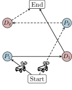
From a mathematical perspective, this communication can be modeled by means of a time-varying digraph , where is a universal slotted time representing temporal information on the graph evolution, while represents the set of edges of . A digraph models inter-robot communications in the sense that there is an edge if and only if robot can send information to robot at time . In this tutorial, we will denote the set of in-neighbors of robot at time by , that is, the set of such that there exists an edge (cf. Figure 1). We now recall basic properties from graph theory which will be used in the rest of the tutorial. If does not depend on the time , then the graph is called static, otherwise, it is called time-varying. A graph is said to be undirected if for each edge at time it stands at time . Otherwise, the graph is said to be directed and is also called digraph. A static digraph is said to be strongly connected if there exists a directed path connecting each pair . A time-varying digraph is said to be jointly strongly connected if, for all , the graph constructed as is strongly connected. Finally, is said to be -strongly connected if there exists an integer such that, for all , the graph defined as is strongly connected.
II-B Hardware-Software Implementation: a ROS-2 perspective
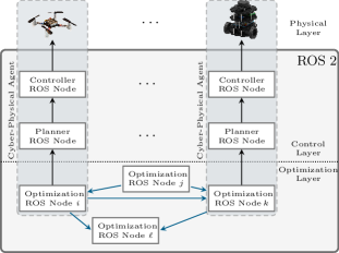
In real experiments, robots are controlled by a set of inter-communicating processes. These processes may read data from sensors, implement decision, planning, and control schemes, and may exchange data with other robots or with the environment by means of, e.g., WiFi communication. Following this line, in this tutorial, we consider each robot as a cyber-physical system in which the aforementioned actions are performed by a set of ROS 2 independent processes (also called nodes). In ROS 2, nodes can be deployed on independent computing units and can exchange data according to different protocols. We focus on the publish-subscribe protocol in which nodes can act in two ways, i.e., publisher and subscriber. When a node acts as a publisher, it sends data over a dedicated topic on the TCP/IP stack. Nodes interested in the data can then subscribe to the topic to receive it as soon as it is published. Nodes can act simultaneously as publishers and subscribers on different topics (cf. Figure 1). Moreover, they can change almost at run-time the topics they are subscribed to. Interestingly, ROS 2 implements a broker-less publish-subscribe protocol in which nodes are able to find and exchange data without the need for a central coordinating unity. We refer the reader to Figure 1 for an illustrative example.
III Consensus Optimization
and Partition-Based Optimization
In this section, we briefly recall the consensus optimization and partition-based optimization frameworks. As we detail next, these two frameworks have been extensively studied from a theoretical perspective. Thus, in this paper we briefly recall them and, instead, we focus on two other setups that model a larger set of multi-robot scenarios.
III-A Consensus Optimization
In the so-called consensus optimization setup, the objective is to minimize the sum of local functions , each one depending on a global variable , i.e.:
| (1) | ||||
In more general versions of this setup, the set can be defined as the intersection of local constraint sets . In this setup, robots usually update local solution estimates that eventually converge to a common optimal solution to (1). This setup is particularly suited for decision systems performing data analytics in which data are private and the consensus has to be reached on a common set of parameters characterizing a global classifier or estimator (e.g., neural network) based on all data. This setup has been investigated in several papers for decision-making in multi-agent systems, see, e.g., [4, 14, 15, 88, 1, 2, 87, 3, 85, 16, 86] for detailed dissertations. In cooperative robotics, this scenario can be interesting to reach a consensus on a common quantity, e.g., target estimation. We refer the reader to the survey [16] that is centered around this optimization setting.
III-B Partition-Based Optimization
This framework models problems with a partitioned structure. More in detail, let the decision vector be in the form . Here, and . The subset represents information related to robot . Assume that robots communicate according to a static connected, undirected graph. The partition-based optimization framework assumes that the objective functions and the constraints have the same sparsity structure as the communication graph. That is, the function and the constraint set depend only on and on for all . Thereby, partition-based optimization problems are in the form
| (2) | ||||
This framework has been extensively analyzed from a theoretical perspective, see, e.g., [89, 90, 91, 92]. However, this setup is strictly related to application scenarios in which the sparsity of the communication can match the one of functions and constraints. In this tutorial instead, we consider more general application scenarios in which the formulation is independent of the network structure. Indeed, in multi-robot applications, the communication topology may be not related to the optimization sparsity and it may vary during time due to robot movements.
IV Constraint-Coupled Optimization Setup
for Cooperative Robotics
In this distributed optimization framework, robots aim at minimizing the sum of local cost functions , each one depending only on a local decision vector . The decision vectors of the robots are coupled by means of separable coupling constraints . Distributed constraint-coupled optimization problems can be formalized as
| (3) | ||||
An example of a constraint-coupled linear program with and for each is provided in Figure 2.
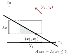
In this distributed setup, the size of the entire decision vector , usually increases with the number of robots in the network. Thus, scalable distributed optimization algorithms are designed so that the generic robot only constructs its local, small portion of the optimal decision vector .
IV-A Multi-Robot Constraint-Coupled 1: Multi-Robot Task Allocation
In this section, we consider a scenario in which a team of robots has to negotiate how to optimally serve a set of tasks, see, e.g., [53] for a detailed discussion. This task allocation problem is a notable example of constraint-coupled optimization. Here, we focus on a linear assignment problem. Consider a network of robots, that has to serve a set of tasks. The generic robot incurs a cost if it serves task . Moreover, each robot may be able to serve only a subset of the tasks. A graphical representation is given in Figure 3.
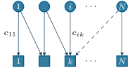
The objective is to find a robot-to-task assignment such that all the tasks are served, each robot serves one task and the overall cost is minimized. Let be the set of tuples defined as . To each robot it is associated a binary decision vector with . The -th entry of is equal to if the robot serves task and otherwise. Let be the vector stacking the costs . The constraint that each robot has to serve one task can be enforced by the following . Let be a matrix obtained by extracting from a identity matrix all the columns such that . Then, the linear assignment problem can be written as an integer linear program in the form
| (4) | ||||
It is worth noting that the linear assignment is a special case of the constraint-coupled optimization problem in which the coupling constraint is a linear, equality constraint. It is immediate to see that, considering and it is possible to recover the structure of problem (3). Moreover, exploiting the so-called unimodularity of the constraint matrices, the local sets can be replaced with linear, convex sets in the form . In this way, the task assignment can be solved as a linear program.
IV-B Multi-Robot Constraint-Coupled 2: Planning of Battery Charging for Electric Robots
Inspired by the application proposed in [93], we consider a charging scheduling problem in a fleet of battery-operated robots drawing power from a common infrastructure. This schedule has to satisfy local requirements for each robot, e.g., the final state of charge (SoC). The schedule also has to satisfy power constraints, e.g., limits on the maximum power flow. We assume that charging can be interrupted and resumed. The overall charging period is discretized into time steps. For each robot , let be a set of decision variables handling the charging of the robot. That is robot charges at time step with a certain charge rate between (no charging) and . The -th battery charge level during time is denoted by . The -th battery initial SoC is and, at the end of the charging period, its SoC must be at least .
We denote by and the battery’s capacity limits, by the maximum charging power that can be fed to the -th robot, and by the maximum power flow that robots can draw from the infrastructure. Let be the price for electricity consumption at time slot . Let denote the set . The objective is to minimize the cost consumption. Then, the optimization problem can be cast as
| (5a) | ||||||
| subj. to | (5b) | |||||
| (5c) | ||||||
| (5d) | ||||||
| (5e) | ||||||
| (5f) | ||||||
| (5g) | ||||||
In order to cast (5) as a constraint-coupled optimization problem, let us define the following quantities. For each robot , let be the stack of . Also, let be the stack of . Then,
| (6) |
where is a suitable vector in the form . As for the local constraints, let us define for all the set
| (7) |
Finally, all the local variables are coupled by the constraint (5b).
IV-C Multi-Robot Constraint-Coupled 3: Multi-Robot Pickup-and-Delivery
Inspired by the work [42], we consider a network of robots that have to serve a number of pickup and delivery requests. That is, robots have to pick up goods at some locations and deliver them to other locations. We denote by denote the index set of pickup requests, while delivery requests are denoted as . A good picked up at location must be delivered at . This enforces that the two requests have to be served by the same robot. Let be the set of all the requests. The objective is to serve all the requests by minimizing the total traveled distance, see Figure 4 for an example.
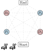
Each request is characterized by a service time , which is the time needed to perform the pickup or delivery operation. Within each request, it is also associated a load , which is positive if and negative if . Each robot has a maximum load capacity of goods that can be simultaneously held. The travel time needed for the -th robot to move from a location to another location is denoted by . In order to travel from two locations , the -th robot incurs a cost . Finally, two additional locations and are considered. The first one represents the mission starting point, while the second one is a virtual ending point. For this reason, the corresponding demands and service times are set to . The goal is to construct minimum-cost paths satisfying all transportation requests. To this end, a graph of all possible paths through the transportation requests can be defined. We underline that this graph models the optimization problem and it is not related to the graph modeling inter-robot communication. Let , be the graph with vertex set and edge set . contains edges starting from or from locations in and ending in or other locations in (cf. Figure 4). For all edges , let be a binary variable denoting whether robot is traveling () or not () from a location to a location . Also, let be an the optimization variable modeling the time at which robot begins its service at location . Similarly, let be the load of robot when leaving location . The PDVRP can be formulated as the following optimization problem,
| (8a) | ||||
| subj. to | (8b) | |||
| (8c) | ||||
| (8d) | ||||
| (8e) | ||||
For the sake of presentation, we do not report the explicit form of all the constraints. We refer the reader to [94] for the detailed formulation. The PDVRP problem can be cast as a constraint-coupled problem (3) as follows. For each , let be the stack of all the for all . Similarly, let be the stack of all the for all . Finally, let be the stack of . With this notation at hand, it stands
| (9) |
Note that the constraints (8c)–(8e) are repeated for each index . Thus, let us define for all the set
| (10) |
Finally, notice that (8b) is a constraint coupling the variables of all the robots. Thereby, we model them by setting
| (11) |
V Aggregative Optimization Setup for Cooperative Robotics
The aggregative optimization setup has been originally introduced in the pioneering works [95, 96] in which first distributed algorithms have been provided. Such a framework suitably models applications in which the robots take decisions by simultaneously considering their local evolution and an aggregative behavior of the network. Formally, in this setup, the robots are interested in minimizing the sum of local cost functions but, differently from the constraint-coupled framework (cf. Section IV), each local function depends both on (i) the associated decision variable and (ii) an aggregation of all the decision variables of the network, for a suitable function . That is, the aggregative optimization problem is defined as
| (12) | ||||
where, for all , is the objective function of robot , its feasible set, and, given , the aggregative variable reads as
where is the -th contribution to the aggregative variable. According to the distributed paradigm, we assume each robot is aware only of , and , thus not having knowledge of other robot data.
V-A Multi-Robot Aggregative 1: Target Surveillance
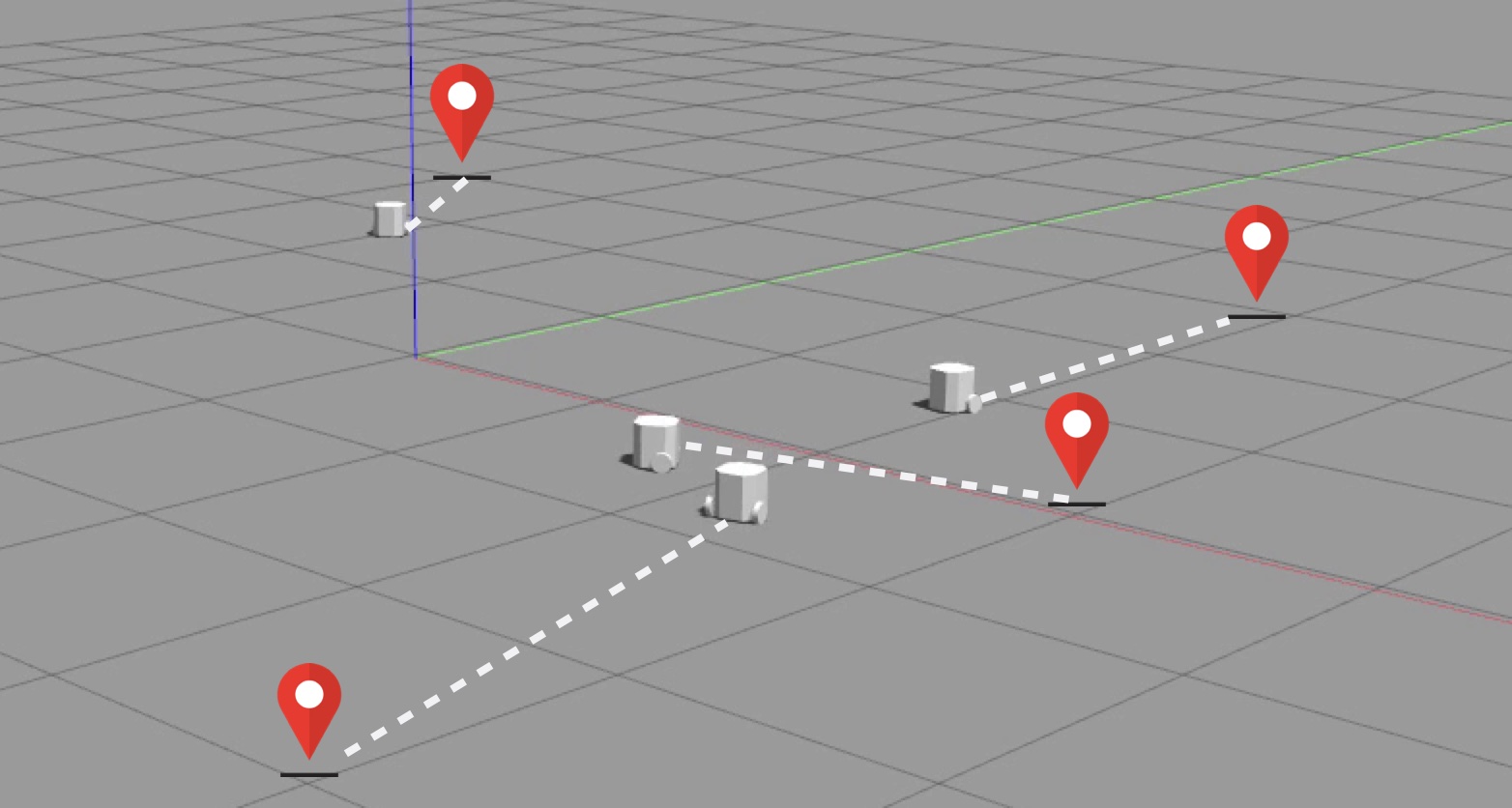
We now introduce a motivating example, namely the Target Surveillance problem, that can be cast into a distributed aggregative optimization problem. An illustrative example is given in Figure 5.
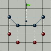
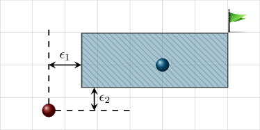
In this scenario, a team of robots has to protect a target from a set of intruders. We denote by the position of robot and by the position of the target. Each robot wants to stay as close as possible to its designated intruder, but simultaneously not to drift apart from the target so as not to leave it unprotected. Moreover, we impose that each defending robot poses itself between the corresponding intruder and the target to protect. A 2D example of this constraint set is shown in Figure 6.
In this setting, we assume that each robot only knows its position and the position of the -th intruder. Hence, the resulting strategy for the target-surveillance problem can be chosen by solving the optimization program
| (13a) | ||||
| subj. to | (13b) | |||
| (13c) | ||||
In (13a), are scaling parameters, while, in the constraints (13b) and (13c), we used to denote the -th component of the vectors and to denote an additional tolerance. Problem (13) can be cast as an instance of the aggregative optimization problem (12) as follows. First, notice that the cost (13a) can be split into the sum of functions. Each one of them depends on a local variable and on an aggregated term
with . Thus,
Finally, note that constraints (13b) and (13c) are local for each robot. Therefore, is it possible to define for each
V-B Multi-Robot Aggregative 2: Multi-Robot Resource Allocation with Soft Constraints
Here, we consider a version of the Multi-Robot Resource Allocation in which we relax the resource allocation constraint and we handle it through a suitable recasting into a distributed aggregative optimization problem. In this scenario, a team of robots have to cooperatively perform a set of individual tasks by relying on a common, finite resource. Specifically, we denote by be the portion of resource allocated to robot to perform its individual tasks. Then, we denote with the utility function used to measure the quality of the service provided by robot in performing its individual task. Moreover, it is desirable to not exceed a certain bound about the aggregate allocated resource , so that a penalty function depending on is added to the cost. We remark that, here, differently from more standard resource allocation formulations, it is possible to exceed such a bound because it is not modeled through a hard constraint. Further, we assume that each quantity is constrained to satisfy a bound in the form , for some . Therefore, we can model this allocation problem through the program
| (14a) | ||||
| subj. to | (14b) | |||
The objective function in (14a) can be split into the sum of functions depending on the local variable and the aggregated term . Therefore, the aggregative structure (12) is recovered by setting each local function as
where and, thus, each aggregation rule as
Finally, we impose the (local) constraints (14b) by defining, for each robot , the (local) feasible set defined as
VI Distributed Methods for Constrained-Coupled Optimization
In this section, we describe two algorithms to address constraint-coupled optimization problems in the form (3), namely the Distributed Dual Decomposition, [97], and the Distributed Primal Decomposition, [98]. The algorithms address convex optimization problems, but suitable extensions can be designed to handle mixed-integer linear programs, [93, 98].
VI-A Distributed Dual Decomposition
Given optimization problems as in (3), let us define the Lagrangian function, ,
with the vector of Lagrange multipliers. With this definition at hand, it is possible to define the (concave) dual function as
By exploiting the structure of the Lagrangian, it turns out that with
| (15) |
Thus, we can define the dual problem of (3) as
| (16) |
As discussed in [99], the dual of a constraint-coupled problem has a consensus optimization structure. In [97], a distributed algorithm based on a distributed proximal on the dual is proposed. This scheme is reported in Algorithm 1 from the perspective of robot .
We now briefly explain the main steps in Algorithm 1. Each robot initializes its portion of the solution vector estimate as , and the dual vector estimate with a feasible solution to problem (16). More details on the initialization procedure can be found in [97]. At every iteration , each robot computes a weighted average of the dual vector based on its own estimate and on neighbor estimates , . Then, it updates by minimizing the local term of the Lagrangian function evaluated at , and via a proximal minimization step. It can be shown that may not converge to the optimal solution to (3). Therefore, each robot computes a local candidate solution as the weighted running average of , i.e.,
| (17) |
This procedure is often referred to as the primal recovery procedure of dual decomposition [100, 101, 102]. It is worth noting that robots do not exchange any information on their local estimates . Indeed, robots only exchange local dual estimates. This is an appealing feature in privacy-preserving settings.
The main convergence result for Algorithm 1 requires the following assumptions.
Assumption VI.1.
For each , the functions and each component of are convex. Also, for each the sets are convex and compact.
Assumption VI.2.
There exists , in the relative interior of the set , such that for those components of that are linear in , if any, while for all other components.
Assumption VI.3.
is a non-increasing sequence of positive reals such that for all . Also,
-
(i)
,
-
(ii)
.
Assumption VI.4.
There exists such that for all and all , , , and implies that . Moreover, for all ,
-
(i)
for all ,
-
(ii)
for all .
Assumption VI.5.
Let and let . Then, the graph is strongly connected, i.e., for any two nodes there exists a path of directed edges that connects them. Moreover, there exists such that for every , robot receives information from a neighboring robot at least once every consecutive iterations.
The main convergence result is as follows.
Theorem VI.6.
Remark VI.7.
An effective approach to improve the numerical robustness of dual decomposition is the well-known (centralized) algorithm named Alternating Direction Method of Multipliers (ADMM). A distributed version of ADMM is provided in [103], where a dynamic average consensus protocol is suitably embedded in the parallel version to track missing global information. Indeed, to solve (3), the parallel ADMM would require the knowledge of the coupling constraint violation, which is a global quantity not available at each robot.
VI-B Distributed Primal Decomposition
Primal decomposition is a powerful tool to recast constraint-coupled convex programs such as (3) into a master-subproblem architecture, [104]. In the following, we consider coupling constraints in the form111We introduced the constraint-coupled setup with coupling constraints in the form . The additional, constant term in this section can be easily embedded into the functions . , with . The main idea is to interpret the right-hand side vector as a limited resource that must be shared among robots. Thus, for all we introduce local allocation vectors satisfying . With these new variables, problem (3) can be equivalently restated as
This problem can be rewritten as a master-subproblem architecture. Specifically, robots cooperatively solve a so-called master problem, in the form
| (20) | ||||
Here, for each , is defined as the optimal cost of the -th subproblem, i.e.
| (21) | ||||
In problem (20), the constraint defines the set of feasible solutions for problem (24). Given an optimal allocation , each robot can reconstruct its portion of the optimal solution for problem (3) by using its corresponding local allocation .
In [105, 106], authors propose distributed primal decomposition schemes to address constraint-coupled convex problems. In the remainder of this section, we focus on a challenging mixed-integer setup, and we introduce a tailored distributed primal-decomposition scheme to solve it [98]. Then, we discuss in a remark how the algorithm can be customized to address convex problems. In [98] authors provide numerical simulations showing that this distributed decomposition scheme allows for the solution of a larger set of problems and achieves better sub-optimality bounds with respect to distributed duality decomposition schemes.
The distributed optimization algorithm proposed in [98] addresses mixed-integer programs in the form
| (22) | ||||
Here, the decision variable of the generic robot has components and the constraint set is of the form , where is a non-empty, compact polyhedron. The decision variables are coupled by linear constraints, described by the matrices and the vector . Following [93, 107, 108, 109], the idea is to solve a convex, relaxed version of (22) in the form
| (23) | ||||
where for all and denotes the convex hull of . The restriction is designed to guarantee that (23) admits a solution. More details are provided in [98]. Once an optimal solution has been found, the optimal solution to (22) can be reconstructed. With this reformulation at hand, the idea is to exploit a primal decomposition approach. To this end, robots cooperatively solve a so-called master problem, in the form of (20), with subproblems in the form
| (24) | ||||
The algorithm, from the -th robot perspective, is summarized in Table 2, where is the step-size, and means that the variables , and are minimized in a lexicographic order [4]. In Algorithm 2, the generic robot maintains a local allocation estimate , and reconstructs a local feasible solution to the original problem (22).
| (25) | ||||
Remark VI.8.
A distributed primal decomposition algorithm for (nonlinear) convex constraint-coupled problems can be obtained from Algorithm 2 as follows. In the Compute step, together with the multiplier , each robot also stores a candidate solution to the local subproblem. The sequence can be shown to converge to a feasible solution to (3). The final solution step of (25) is then not required [105, 106].
Algorithm 2 can be shown to achieve finite-time feasibility under the following assumptions.
Assumption VI.9.
The step-size sequence , with each , satisfies , .
Assumption VI.10.
For a given , the optimal solution of problem (23) is unique.
Assumption VI.11.
For a given , there exists a vector , with for all , such that
| (26) |
The cost of is denoted by .
Let denote an a-priori restriction computed as described in [98]. Then, the main result can be stated as follows.
Theorem VI.12 ( [98]).
VII Distributed Methods for Aggregative Optimization
In this section, we describe two schemes to address aggregative optimization problems in the form (12). The Projected Aggregative Tracking proposed in [110] (as a modified scheme of the one introduced in [96]) is a distributed scheme inspired by a projected gradient method. The Distributed Frank-Wolfe Algorithm with Gradient Tracking proposed in [111] is instead inspired by the so-called Franke-Wolfe update. Recently, in [112] a distributed feedback law for aggregative problems is designed in the context of feedback optimization. Finally, in [113], the aggregative framework is addressed via an ADMM-based algorithm.
VII-A Projected Aggregative Tracking
The algorithm in [110] consists of maintaining in each robot , at each iteration , an estimate about the -th block of a solution to problem (12). In order to update such an estimate, one may use the projected gradient method. In each robot , such a method would require the knowledge of the derivative of with respect to computed in the current configuration . In light of the chain rule, such a quantity reads as
| (27) |
Computing the quantity (27) would require the knowledge of the global quantities and . To overcome this issue, robot resorts to two auxiliary variables called trackers compensating for the local lack of knowledge. Specifically, robot exploits neighboring communication to update the trackers according to two suitable perturbed consensus dynamics. The whole fully-distributed procedure is summarized in Algorithm 3 where are the weights of a weighted adjacency matrix associated to the graph, is the step-size, while is a convex combination constant.
The main convergence result for Algorithm 3 requires the following assumptions where, for the sake of readability, we adopt , , and defined as
where and with and for all .
Assumption VII.1.
The graph is undirected and connected and is doubly stochastic.
Assumption VII.2.
For all , is nonempty, closed, and convex, while the global objective function is -strongly convex.
Assumption VII.3.
The function is differentiable with -Lipschitz continuous gradients, and , are Lipschitz continuous with constants , respectively. For all , the aggregation function is differentiable and -Lipschitz continuous.
The following theorem guarantees the linear convergence of Algorithm 3 to the (unique, cf. Assumption VII.2) solution to problem (12).
Theorem VII.4 ([110]).
A first, pioneering version of Algorithm 3 was proposed in [95] for the static, unconstrained setting. A first version for the online, constrained setting was introduced in [96], whose continuous-time counterpart has been extended in [114] to deal with quantized communication. In [115], Algorithm 3 has been combined with a Recursive Least Squares mechanism to learn unknown parts of the objective functions in a personalized setting. It is worth noting that Algorithm 3 achieves linear convergence (cf. Theorem VII.4) in solving problem (12). As for the unconstrained setting, the linear convergence is also achieved by the distributed method proposed in [95], its extension in [111] dealing with quantized communication, and its accelerated versions proposed in [116].
VII-B Distributed Frank-Wolfe Algorithm with Gradient Tracking
The algorithm in [111] is inspired by the so-called Franke-Wolfe method. The main difference between the projected gradient method and the Franke-Wolfe method lies in the fact that the latter, at the cost of loosing linear convergence, requires a lower computational cost. When applied to problem (12), in each robot , the Franke-Wolfe method reads as
| (28a) | ||||
| (28b) | ||||
where is the time-varying step-size at iteration , while, in order to ease the notation, we introduced to denote the derivative of computed at , namely
As in Section VII-A, the presence of global, unavailable quantities required to compute makes the update (28) not implementable in a distributed fashion. For this reason, the update (28) is modified and suitably interlaced with two trackers and having the same role and dynamics as in Section VII-A. The whole procedure is named Distributed Frank-Wolfe Algorithm with Gradient Tracking and is summarized in Algorithm 4. In [111], the algorithm has been studied to deal with time-varying graphs . Indeed, we notice that the trackers’ updates depend on time-varying weights corresponding to a time-varying adjacency matrix associated to .
We state suitable assumptions to provide the convergence result related to Algorithm 4.
Assumption VII.5.
For each robot , the feasible set is closed, convex, and compact, while the global objective function is convex and differentiable over .
Assumption VII.6.
is doubly stochastic for all . Moreover, there exists a constant such that for all , , and . Further, there exists such that the union graph is strongly connected for all .
Assumption VII.7.
For all , it holds , , and .
VIII Toolboxes and Experiments
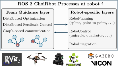
To further highlight the potentialities of the considered frameworks in multi-robot applications, in this section we provide simulations and experiments on teams of robots for the proposed theoretical settings. The implementation of the distributed algorithms has been performed using the DISROPT Python package [83]. This framework allows users to implement distributed algorithms from the perspective of the generic robot in the network and provides API to exchange data according to user-defined graphs. The implementation on the robotic platform instead is performed using ChoiRbot [82], and CrazyChoir [84], two novel ROS 2 frameworks tailored for multi-robot applications. Specifically, ChoiRbot is a general-purpose framework allowing for the implementation of distributed optimization and control schemes on generic robots, whereas CrazyChoir is tailored to manage Crazyflie nano-quadrotor fleets. Both frameworks are based on the ROS 2 framework. Each robot is modeled as a cyber-physical agent and consists of three interacting layers: distributed optimization layer, trajectory planning layer, and low-level control layer. For each robot, each layer is handled by a different ROS 2 process. As for the distributed optimization layer, the two frameworks support the implementation of algorithms using DISROPT, and implement inter-robot communication using the inter-process communication stack of ROS 2. To better clarify this structure, we report the ChoiRbot architecture in Figure 7. Here, it is possible to see how these toolboxes allow for the implementation of distributed algorithms in a flexible and scalable fashion. It is worth noting that, in these frameworks, low-level planning and control are independent of the implementation of distributed algorithms. In this way, users can also resort to existing low-level control routines to actuate the robots. Moreover, the toolboxes allow for seamless integration with external simulators, e.g., Gazebo [117] or Webots [118], and allow users to switch from simulation to experiments by changing a few lines of code.
.
In the ROS 2 framework, communication is implemented via a publish-subscribe protocol, enabling message exchange among different computing units connected across the network. Leveraging this feature, the experiments are performed over a real WiFi network, thus taking into account delays and asynchronous (or lossy) communications over a given, user-defined communication graph.
VIII-A Experiments for Multi-Robot Constraint-Coupled 1
In the following, we provide Gazebo simulations on a team of TurtleBot 3 Burger mobile robots tackling a task allocation problem as in Section IV-A by using the Dual Decomposition scheme in Algorithm 1. In the considered scenario, robots have to fulfill tasks, randomly scattered in the environment. For the sake of simplicity, we assume that a task is accomplished once the allocated robot reaches its position. To solve the optimization problem, robots communicate according to an Erdős-Rényi random graph with edge probability . Following the setup described in [82], we consider the scenario in which more tasks arrive during time. We assume that a new task is revealed as soon as robots complete an already-known task. As soon as robots receive information on new tasks, they restart the optimization procedure and evaluate a novel, optimal allocation. As soon as robots finish the optimization, they start moving toward their designated task. To this end, we have a proportional control scheme. To avoid collisions, the control inputs are fed into a collision avoidance scheme using a barrier function as in [77]. In Figure 8, we provide a snapshot of the simulation222A video of the simulation is available at https://youtu.be/9YzbdmIgCYg..
VIII-B Simulations for Multi-Robot Constraint-Coupled 2
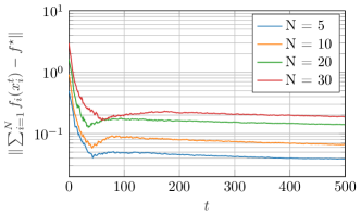
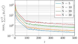
In this section, we provide numerical simulations for the constraint-coupled optimization setup described in Section IV-B. The distributed algorithm has been implemented using DISROPT from the perspective of the -th robot as in Algorithm 1. In DISROPT, each robot is simulated using an isolated process. Different processes communicate according to a user-defined graph using the MPI (Message Passing Interface) protocol. We run a Monte Carlo simulation for a different number of robots. That is, we considered the cases with . Robots are connected according to an Erdős-Rényi random graph with edge probability . For each case, we run different simulations with varying parameters. More in detail, we assumed a charging period of time slots, with each time slot having a duration of minutes. All the other quantities in (5) have been generated according to [93]. During each simulation, we run the algorithm for iterations. Then, we evaluated the maximum for each iteration over the simulations. Results are provided in Figure 9. Here, we provide the cost error and the violation of the coupling constraints. As expected from theory, robot estimates converge towards the optimal value, and the violation of the coupling constraints approaches .
VIII-C Experiments for Multi-Robot Constraint-Coupled 3
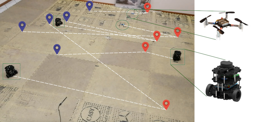
In the next, we report the results of an experiment for the pickup-and-delivery problem solved using the Distributed Primal Decomposition scheme summarized in Algorithm 2, [42]. We consider an experimental setting in which a pickup and delivery tasks must be served by a team of robots. A task is considered accomplished once the designated robot reaches the task position. To simulate the load/unload of goods in classical pickup-and-delivery settings, robots have to wait on the task for a certain random time, which is drawn uniformly between and seconds. Also, each robot can serve only a subset of the overall number of tasks. The designated robotic fleet is composed of Crazyflie nano-quadrotors and TurtleBot3 Burger mobile robots. As for the low-level control routines, we follow the setting discussed in Section VIII-A to avoid collisions among mobile, ground robots. As for the quadrotors instead, we implemented a flatness-based hierarchical control scheme. A snapshot from the experiment is provided in Figure 10. 333A video can be found at https://youtu.be/NwqzIEBNIS4..
VIII-D Experiments for Multi-Robot Aggregative 1
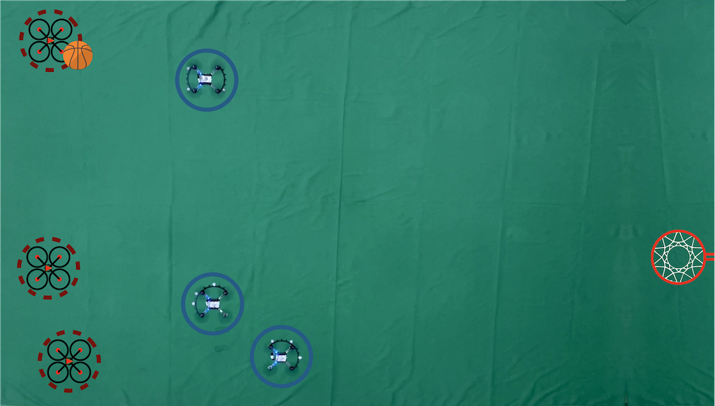
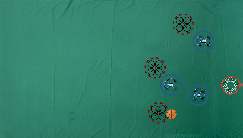
Here, we report the experiments provided in [119]. Specifically, we develop the experimental setting in Section V-A as a multi-robot basketball match. The scenario unfolds as follows. A fleet of robots plays the role of the defending team, with the defensive strategy modeled as an aggregative optimization problem. The offending team, also composed of robots, moves following pre-defined trajectories. In this setting, the optimization variable models the position of robot at time . Each robot has to man-mark a robot in the offending team, whose position is denoted as . The position of the ball, known by all the robots, is denoted by . Similarly, the position of the basket is denoted by . The generic robot in the defending team aims at placing over the segment linking and . Also, robots in the defending team want to steer their barycenter on the segment linking the basket and the ball. This strategy can be cast as an aggregative optimization problem in the form of (12), with objective functions
| (29) |
where . Also, models a point on the segment connecting the basket and the -th offensive player. Similarly, models a point on the segment connecting the ball to the basket. It is worth noting that, differently from the setup in Section V, the cost function (29) has also a term taking into account the position of other neighboring robots. This particular function models a barrier to avoid inter-robot collisions in the defending team. In the proposed experiments, we choose as robotic platform the Crazyflie nano-quadrotor. Intruders are virtual, simulated quadrotors. The described setup is tackled by implementing a distributed method, proposed in [119], extending Algorithm 3 to deal with (i) time-varying networks and (ii) the barrier functions. Moreover, in order to predict the updated positions of the target and the intruders, a Kalman-based mechanism is interlaced with the optimization scheme. A snapshot from an experiment is in Figure 11 444The video is available at https://www.youtube.com/watch?v=5bFFdURhTYs..
VIII-E Simulations for Multi-Robot Aggregative 2
In this section, we provide numerical simulations addressing the multi-robot resource allocation scenario described in Section V-B, i.e., the one formulated as an instance of the aggregative optimization problem as given in (12). To tackle this problem in a distributed fashion, we implement Algorithm 3 and Algorithm 4 (cf. Section VII). The numerical simulation is organized as follows. A team of robots cooperatively allocates a common, scalar resource according to a common performance criterion. Specifically, the robots have to perform a set of individual tasks and, for each robot , there is a quadratic utility function assessing the quality of of the service provided by robot according to
| (30) |
where and for all . Further, given , the penalty function is defined as
Therefore, for all , the local objective function reads as
Moreover, each quantity is constrained to belong to for some . For all , the parameters and are randomly generated extracting them, with uniform probability, from the intervals and , respectively. Then, we set and . As for the communication among the robots of the network, we randomly generate an undirected, connected Erdős-Rényi graph with parameter and an associated doubly stochastic weighted adjacency matrix. As for the algorithm parameters, we implement (i) Algorithm 3 choosing , and (ii) Algorithm 4 choosing . Figure 12 reports the performance of the algorithms in terms of the convergence of the relative optimality error , where is the (unique) solution to the considered problem.
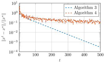
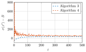
As predicted by Theorem VII.4 and VII.8, Figure 12 shows that both Algorithm 3 and 4 converges toward but the linear convergence is only achieved by Algorithm 3. Finally, in Figure 13, we report the evolution over of the quantity achieved by running Algorithm 3 and 4. As one may expect, such a quantity is not necessarily negative because exceeding configurations are not forbidden but only penalized.
IX Research Directions
In this section, we present some research directions extending the scenarios considered in this tutorial.
Imperfect communication protocols
In several applications involving networks of robots, assuming a perfectly synchronous and reliable communication protocol among robots may be not realistic. For this reason, it would be useful to either design reliable communication protocols or design algorithms that are robust with respect to asynchronous exchanges and/or packet losses in the communication among robots. In an asynchronous setting, each robot updates and/or sends its local quantities in a totally asynchronous fashion with respect to the other robots of the network. In the distributed optimization literature, such a setting has already gained attention from a theoretical point of view but mainly in the consensus optimization setup, see, e.g., [120, 91, 90, 121, 122, 123, 124, 125, 126]. As for networks with packet losses, they are often modeled by considering that a message sent by robot is successfully received by robot with a given probability. Preliminary theoretical results dealing with networks subject to packet losses are available in [127, 128, 129, 124]. Several challenges are still open at a theoretical level for the presented (constraint-coupled and aggregative) optimization frameworks. Moreover, handling realistic communication models in specific robotic applications is mainly an open problem.
Unknown functions and personalized optimization scenarios
There has been in the last years an increasing interest in scenarios in which the objective function is completely or partially unknown. These scenarios arise, e.g., when robots take measurements via onboard sensors and the function profile is not explicitly available. When functions are not known, gradient-based algorithms are not implementable. To overcome this issue, extremum-seeking and zero-order techniques have been proposed to solve the optimization problem. Several applications have been considered, including, e.g., source seeking [130, 131] and resource allocation [132, 133], object manipulation [134], and trajectory planning [135, 136]. These algorithms have been studied from a theoretical perspective in the distributed framework, [137, 138, 139, 140, 141, 142]. However, there are few applications of these distributed methodologies in multi-robot settings. Another interesting scenario arises when a portion of the local functions is known, while another part related to, e.g., user preferences is unknown. In robotics, this may be due to the presence of humans, interacting with robots, that introduce non-engineering cost functions in the optimization problem. Addressing this scenario for the constraint-coupled and aggregative optimization frameworks discussed in Sections IV and V is an open research direction.
For the constraint-coupled scenario, the cost function in problem (3) becomes , where and are respectively the known and unknown parts of the local objective function of robot . Analogously, for the aggregative framework, the cost function in problem (12) becomes , with the same meaning for the two functions. Interesting examples in robotics can be found, e.g., in the context of trajectory generation [143, 144, 145], rehabilitation robots [146], and demand response tasks in energy networks [147, 148]. Here, human preferences are hard to model and, thus, a possible strategy to deal with them consists in resorting to the so-called personalized approach, i.e., to progressively estimate the unknown objective function by using human feedback. In a centralized setting, personalized optimization has been originally addressed in [149, 150]. As for the distributed setup, personalized strategies are used in [151] to deal with consensus optimization problems and in [115] to address the aggregative scenario. Finally, in [152], the personalized framework is addressed in the context of game theory.
Online and stochastic scenarios
Many applications arising in robotic scenarios occur in dynamic environments and, hence, need to be formalized by resorting to online and/or stochastic problems. Indeed, in the online setup, the cost function and constraints vary over time. That is, for the constraint-coupled setup we have , and , which are revealed to robot only once its decision has been taken. Similarly, for the aggregative case , and . The goal is to design algorithms involving at each only one iteration step (e.g., a gradient update) without solving the entire problem revealed at . In this context, algorithms are evaluated through the dynamic regret, , performance metrics. For the constraint-coupled framework, reads as
where denotes the time horizon, while and denote respectively the minimizer of and the corresponding robots’ estimate for all . Analogously, for the aggregative setting, is defined as
Distributed algorithms for online constraint-coupled optimization can be found in [153, 154, 155, 156, 157, 158], while for online aggregative problems can be found in [96, 110, 115, 119]. In the stochastic versions of the above problems, the variation over of these functions and sets is due to the realization at iteration of a stochastic process, see, e.g.,[159] for the constraint-coupled framework or [96] for the aggregative one.
Recently, in the context of online and/or stochastic optimization, novel methods embedding prediction schemes have gained attention for centralized settings [160, 161, 162, 163]. Designing distributed optimization algorithms for the above frameworks is an interesting research direction. Moreover, implementing enhanced schemes in multi-robot scenarios is mainly an open problem.
X Conclusion
In this paper, we considered cooperative robotics from the point of view of distributed optimization. Specifically, we focused on constraint-coupled and aggregative optimization setups and showed how to recast several challenging problems arising in multi-robot applications into these distributed optimization settings. Then, for both these setups, we reviewed different distributed algorithms to solve them and provided their convergence properties. Moreover, we revised toolboxes to implement distributed optimization schemes on real, multi-robot networks. To bridge the theoretical analysis and the toolbox presentation, we provided simulations and experiments on real teams of heterogeneous robots for different use cases.
References
- [1] A. Nedić and J. Liu, “Distributed optimization for control,” Ann. Review of Control, Robotics, and Autonom. Systems, vol. 1, pp. 77–103, 2018.
- [2] A. Nedić, A. Olshevsky, and M. G. Rabbat, “Network topology and communication-computation tradeoffs in decentralized optimization,” Proceedings of the IEEE, vol. 106, no. 5, pp. 953–976, 2018.
- [3] A. Nedić, “Distributed optimization over networks,” in Multi-agent Optimization. Springer, 2018, pp. 1–84.
- [4] G. Notarstefano, I. Notarnicola, and A. Camisa, “Distributed optimization for smart cyber-physical networks,” Foundations and Trends® in Systems and Control, vol. 7, no. 3, pp. 253–383, 2019.
- [5] T. Yang, X. Yi, J. Wu, Y. Yuan, D. Wu, Z. Meng, Y. Hong, H. Wang, Z. Lin, and K. H. Johansson, “A survey of distributed optimization,” Annual Reviews in Control, vol. 47, pp. 278–305, 2019.
- [6] J. Park, S. Samarakoon, A. Elgabli, J. Kim, M. Bennis, S.-L. Kim, and M. Debbah, “Communication-efficient and distributed learning over wireless networks: Principles and applications,” Proceedings of the IEEE, vol. 109, no. 5, pp. 796–819, 2021.
- [7] A. G. Dimakis, S. Kar, J. M. Moura, M. G. Rabbat, and A. Scaglione, “Gossip algorithms for distributed signal processing,” Proceedings of the IEEE, vol. 98, no. 11, pp. 1847–1864, 2010.
- [8] X. Yu and Y. Xue, “Smart grids: A cyber–physical systems perspective,” Proceedings of the IEEE, vol. 104, no. 5, pp. 1058–1070, 2016.
- [9] D. K. Molzahn, F. Dörfler, H. Sandberg, S. H. Low, S. Chakrabarti, R. Baldick, and J. Lavaei, “A survey of distributed optimization and control algorithms for electric power systems,” IEEE Transactions on Smart Grid, vol. 8, no. 6, pp. 2941–2962, 2017.
- [10] M. Dorigo, G. Theraulaz, and V. Trianni, “Swarm robotics: Past, present, and future [point of view],” Proceedings of the IEEE, vol. 109, no. 7, pp. 1152–1165, 2021.
- [11] T. Haidegger, S. Speidel, D. Stoyanov, and R. M. Satava, “Robot-assisted minimally invasive surgery—surgical robotics in the data age,” Proceedings of the IEEE, vol. 110, no. 7, pp. 835–846, 2022.
- [12] A. Nanjangud, P. C. Blacker, S. Bandyopadhyay, and Y. Gao, “Robotics and ai-enabled on-orbit operations with future generation of small satellites,” Proceedings of the IEEE, vol. 106, no. 3, pp. 429–439, 2018.
- [13] Y. Rizk, M. Awad, and E. W. Tunstel, “Cooperative heterogeneous multi-robot systems: A survey,” ACM Computing Surveys (CSUR), vol. 52, no. 2, pp. 1–31, 2019.
- [14] O. Shorinwa, T. Halsted, J. Yu, and M. Schwager, “Distributed optimization methods for multi-robot systems: Part i–a tutorial,” arXiv preprint arXiv:2301.11313, 2023.
- [15] ——, “Distributed optimization methods for multi-robot systems: Part ii–a survey,” arXiv preprint arXiv:2301.11361, 2023.
- [16] T. Halsted, O. Shorinwa, J. Yu, and M. Schwager, “A survey of distributed optimization methods for multi-robot systems,” arXiv preprint arXiv:2103.12840, 2021.
- [17] L. E. Beaver and A. A. Malikopoulos, “An overview on optimal flocking,” Annual Reviews in Control, 2021.
- [18] J. Hu, H. Zhang, L. Liu, X. Zhu, C. Zhao, and Q. Pan, “Convergent multiagent formation control with collision avoidance,” IEEE Transactions on Robotics, vol. 36, no. 6, pp. 1805–1818, 2020.
- [19] J. Alonso-Mora, S. Baker, and D. Rus, “Multi-robot formation control and object transport in dynamic environments via constrained optimization,” The International Journal of Robotics Research, vol. 36, no. 9, pp. 1000–1021, 2017.
- [20] A. R. Mosteo, E. Montijano, and D. Tardioli, “Optimal role and position assignment in multi-robot freely reachable formations,” Automatica, vol. 81, pp. 305–313, 2017.
- [21] R. Tron, J. Thomas, G. Loianno, K. Daniilidis, and V. Kumar, “A distributed optimization framework for localization and formation control: Applications to vision-based measurements,” IEEE Control Systems Magazine, vol. 36, no. 4, pp. 22–44, 2016.
- [22] H. Xiao, Z. Li, and C. P. Chen, “Formation control of leader–follower mobile robots’ systems using model predictive control based on neural-dynamic optimization,” IEEE Transactions on Industrial Electronics, vol. 63, no. 9, pp. 5752–5762, 2016.
- [23] G. Notarstefano and F. Bullo, “Distributed abstract optimization via constraints consensus: Theory and applications,” IEEE Transactions on Automatic Control, vol. 56, no. 10, pp. 2247–2261, 2011.
- [24] J. C. Derenick and J. R. Spletzer, “Convex optimization strategies for coordinating large-scale robot formations,” IEEE Transactions on Robotics, vol. 23, no. 6, pp. 1252–1259, 2007.
- [25] R. L. Raffard, C. J. Tomlin, and S. P. Boyd, “Distributed optimization for cooperative agents: Application to formation flight,” in IEEE Conference on Decision and Control, vol. 3, 2004, pp. 2453–2459.
- [26] J. Tordesillas and J. P. How, “Mader: Trajectory planner in multiagent and dynamic environments,” IEEE Transactions on Robotics, vol. 38, no. 1, pp. 463–476, 2021.
- [27] X. Zhang, H. Shen, G. Xie, H. Lu, and B. Tian, “Decentralized motion planning for multi quadrotor with obstacle and collision avoidance,” Intern. Journ. of Intelligent Robotics and Applications, pp. 1–10, 2021.
- [28] J. Li, M. Ran, and L. Xie, “Efficient trajectory planning for multiple non-holonomic mobile robots via prioritized trajectory optimization,” IEEE Robotics and Automation Lett., vol. 6, no. 2, pp. 405–412, 2020.
- [29] J. Park, J. Kim, I. Jang, and H. J. Kim, “Efficient multi-agent trajectory planning with feasibility guarantee using relative bernstein polynomial,” in IEEE International Conference on Robotics and Automation, 2020, pp. 434–440.
- [30] P. Das and P. K. Jena, “Multi-robot path planning using improved particle swarm optimization algorithm through novel evolutionary operators,” Applied Soft Computing, vol. 92, p. 106312, 2020.
- [31] C. Purcaru, R.-E. Precup, D. Iercan, L.-O. Fedorovici, E. M. Petriu, and E.-I. Voisan, “Multi-robot gsa-and pso-based optimal path planning in static environments,” in 9th International Workshop on Robot Motion and Control. IEEE, 2013, pp. 197–202.
- [32] A. C. Kapoutsis, S. A. Chatzichristofis, and E. B. Kosmatopoulos, “Darp: divide areas algorithm for optimal multi-robot coverage path planning,” Journal of Intelligent & Robotic Systems, vol. 86, no. 3-4, pp. 663–680, 2017.
- [33] Z. Wang, M. Li, L. Dou, Y. Li, Q. Zhao, and J. Li, “A novel multi-objective artificial bee colony algorithm for multi-robot path planning,” in IEEE Inter. Conf. on Inform. and Automation, 2015, pp. 481–486.
- [34] S. Riazi, K. Bengtsson, O. Wigström, E. Vidarsson, and B. Lennartson, “Energy optimization of multi-robot systems,” in IEEE Intern. Conference on Automation Science and Engineering, 2015, pp. 1345–1350.
- [35] S. Bhattacharya and V. Kumar, “Distributed optimization with pairwise constraints and its application to multi-robot path planning,” Robotics: Science and Systems VI, vol. 177, 2011.
- [36] R. Luna and K. E. Bekris, “Network-guided multi-robot path planning in discrete representations,” in 2010 IEEE/RSJ International Conference on Intelligent Robots and Systems. IEEE, 2010, pp. 4596–4602.
- [37] A. Benevento, M. Santos, G. Notarstefano, K. Paynabar, M. Bloch, and M. Egerstedt, “Multi-robot coordination for estimation and coverage of unknown spatial fields,” in IEEE International Conference on Robotics and Automation, 2020, pp. 7740–7746.
- [38] A. C. Kapoutsis, S. A. Chatzichristofis, and E. B. Kosmatopoulos, “A distributed, plug-n-play algorithm for multi-robot applications with a priori non-computable objective functions,” The International Journal of Robotics Research, vol. 38, no. 7, pp. 813–832, 2019.
- [39] G. Notomista and M. Egerstedt, “Constraint-driven coordinated control of multi-robot systems,” in IEEE American Control Conference, 2019, pp. 1990–1996.
- [40] N. Karapetyan, J. Moulton, J. S. Lewis, A. Q. Li, J. M. O’Kane, and I. Rekleitis, “Multi-robot dubins coverage with autonomous surface vehicles,” in IEEE International Conference on Robotics and Automation, 2018, pp. 2373–2379.
- [41] J. Cortes, S. Martinez, T. Karatas, and F. Bullo, “Coverage control for mobile sensing networks,” IEEE Transactions on robotics and Automation, vol. 20, no. 2, pp. 243–255, 2004.
- [42] A. Camisa, A. Testa, and G. Notarstefano, “Multi-robot pickup and delivery via distributed resource allocation,” IEEE Transactions on Robotics, vol. 39, no. 2, pp. 1106–1118, 2022.
- [43] F. Bullo, E. Frazzoli, M. Pavone, K. Savla, and S. L. Smith, “Dynamic vehicle routing for robotic systems,” Proceedings of the IEEE, vol. 99, no. 9, pp. 1482–1504, 2011.
- [44] S. D. Bopardikar, S. L. Smith, F. Bullo, and J. P. Hespanha, “Dynamic vehicle routing for translating demands: Stability analysis and receding-horizon policies,” IEEE Transactions on Automatic Control, vol. 55, no. 11, pp. 2554–2569, 2010.
- [45] A. Testa and G. Notarstefano, “Generalized assignment for multi-robot systems via distributed branch-and-price,” IEEE Transactions on Robotics, vol. 38, no. 3, pp. 1990–2001, 2021.
- [46] C. Nam and D. A. Shell, “Robots in the huddle: Upfront computation to reduce global communication at run time in multirobot task allocation,” IEEE Transactions on Robotics, 2019.
- [47] X. Bai, M. Cao, W. Yan, and S. S. Ge, “Efficient routing for precedence-constrained package delivery for heterogeneous vehicles,” IEEE Transactions on Automation Science and Engineering, vol. 17, no. 1, pp. 248–260, 2019.
- [48] A. Testa, A. Rucco, and G. Notarstefano, “Distributed mixed-integer linear programming via cut generation and constraint exchange,” IEEE Transac. on Automatic Control, vol. 65, no. 4, pp. 1456–1467, 2019.
- [49] S. L. Smith and F. Bullo, “Monotonic target assignment for robotic networks,” IEEE Transactions on Automatic Control, vol. 54, no. 9, pp. 2042–2057, 2009.
- [50] S. Chopra, G. Notarstefano, M. Rice, and M. Egerstedt, “A distributed version of the hungarian method for multirobot assignment,” IEEE Transactions on Robotics, vol. 33, no. 4, pp. 932–947, 2017.
- [51] L. Luo, N. Chakraborty, and K. Sycara, “Distributed algorithms for multirobot task assignment with task deadline constraints,” IEEE Transactions on Automation Science and Engineering, vol. 12, no. 3, pp. 876–888, 2015.
- [52] A. Settimi and L. Pallottino, “A subgradient based algorithm for distributed task assignment for heterogeneous mobile robots,” in IEEE Conference on Decision and Control (CDC), 2013, pp. 3665–3670.
- [53] M. Bürger, G. Notarstefano, F. Bullo, and F. Allgöwer, “A distributed simplex algorithm for degenerate linear programs and multi-agent assignments,” Automatica, vol. 48, no. 9, pp. 2298–2304, 2012.
- [54] S. Karaman and G. Inalhan, “Large-scale task/target assignment for UAV fleets using a distributed branch and price optimization scheme,” IFAC Proceedings Volumes, vol. 41, no. 2, pp. 13 310–13 317, 2008.
- [55] D. A. Castanón and C. Wu, “Distributed algorithms for dynamic reassignment,” in IEEE Conference on Decision and Control, vol. 1, 2003, pp. 13–18.
- [56] R. K. Williams, A. Gasparri, and G. Ulivi, “Decentralized matroid optimization for topology constraints in multi-robot allocation problems,” in IEEE Inter. Conf. on Robotics and Automation, 2017, pp. 293–300.
- [57] E. Hartuv, N. Agmon, and S. Kraus, “Scheduling spare drones for persistent task performance under energy constraints,” in Intern. Conf. on Autonomous Agents and MultiAgent Systems, 2018, pp. 532–540.
- [58] G. Torrente, E. Kaufmann, P. Föhn, and D. Scaramuzza, “Data-driven mpc for quadrotors,” IEEE Robotics and Automation Letters, vol. 6, no. 2, pp. 3769–3776, 2021.
- [59] J. Nubert, J. Köhler, V. Berenz, F. Allgöwer, and S. Trimpe, “Safe and fast tracking on a robot manipulator: Robust mpc and neural network control,” IEEE Robotics and Automation Letters, vol. 5, no. 2, pp. 3050–3057, 2020.
- [60] C. Leung, S. Huang, N. Kwok, and G. Dissanayake, “Planning under uncertainty using model predictive control for information gathering,” Robotics and Autonomous Systems, vol. 54, no. 11, pp. 898–910, 2006.
- [61] C. E. Luis, M. Vukosavljev, and A. P. Schoellig, “Online trajectory generation with distributed model predictive control for multi-robot motion planning,” IEEE Robotics and Automation Letters, vol. 5, no. 2, pp. 604–611, 2020.
- [62] M. W. Mehrez, G. K. Mann, and R. G. Gosine, “An optimization based approach for relative localization and relative tracking control in multi-robot systems,” Journal of Intelligent & Robotic Systems, vol. 85, no. 2, pp. 385–408, 2017.
- [63] R. Van Parys and G. Pipeleers, “Distributed mpc for multi-vehicle systems moving in formation,” Robotics and Autonomous Systems, vol. 97, pp. 144–152, 2017.
- [64] T. P. Nascimento, A. P. Moreira, and A. G. S. Conceição, “Multi-robot nonlinear model predictive formation control: Moving target and target absence,” Robotics and Autonomous Systems, vol. 61, no. 12, pp. 1502–1515, 2013.
- [65] T. P. Nascimento, A. G. Conceiçao, and A. P. Moreira, “Multi-robot nonlinear model predictive formation control: the obstacle avoidance problem,” Robotica, vol. 34, no. 3, pp. 549–567, 2016.
- [66] C. Robin and S. Lacroix, “Multi-robot target detection and tracking: taxonomy and survey,” Autonomous Robots, vol. 40, no. 4, pp. 729–760, 2016.
- [67] F. Pasqualetti, A. Franchi, and F. Bullo, “On cooperative patrolling: Optimal trajectories, complexity analysis, and approximation algorithms,” IEEE Transactions on Robotics, vol. 28, no. 3, pp. 592–606, 2012.
- [68] X. Duan and F. Bullo, “Markov chain–based stochastic strategies for robotic surveillance,” Annual Review of Control, Robotics, and Autonomous Systems, vol. 4, pp. 243–264, 2021.
- [69] E. Stump and N. Michael, “Multi-robot persistent surveillance planning as a vehicle routing problem,” in 2011 IEEE International Conference on Automation Science and Engineering. IEEE, 2011, pp. 569–575.
- [70] J. Derenick, J. Spletzer, and A. Hsieh, “An optimal approach to collaborative target tracking with performance guarantees,” Journal of Intelligent and Robotic Systems, vol. 56, no. 1, pp. 47–67, 2009.
- [71] S. Kamath, E. Meisner, and V. Isler, “Triangulation based multi target tracking with mobile sensor networks,” in IEEE International Conference on Robotics and Automation, 2007, pp. 3283–3288.
- [72] Z. Tang and U. Ozguner, “Motion planning for multitarget surveillance with mobile sensor agents,” IEEE Transactions on Robotics, vol. 21, no. 5, pp. 898–908, 2005.
- [73] C. Paxton, A. Hundt, F. Jonathan, K. Guerin, and G. D. Hager, “CoSTAR: Instructing collaborative robots with behavior trees and vision,” in IEEE International Conference on Robotics and Automation, 2017, pp. 564–571.
- [74] V. Grabe, M. Riedel, H. H. Bülthoff, P. R. Giordano, and A. Franchi, “The TeleKyb framework for a modular and extendible ROS-based quadrotor control,” in IEEE European Conference on Mobile Robots, 2013, pp. 19–25.
- [75] J. Meyer, A. Sendobry, S. Kohlbrecher, U. Klingauf, and O. Von Stryk, “Comprehensive simulation of quadrotor uavs using ROS and gazebo,” in International conference on simulation, modeling, and programming for autonomous robots. Springer, 2012, pp. 400–411.
- [76] W. P. N. dos Reis and G. S. Bastos, “Implementing and simulating an alliance-based multi-robot task allocation architecture using ros,” in Robotics. Springer, 2016, pp. 210–227.
- [77] S. Wilson, P. Glotfelter, L. Wang, S. Mayya, G. Notomista, M. Mote, and M. Egerstedt, “The robotarium: Globally impactful opportunities, challenges, and lessons learned in remote-access, distributed control of multirobot systems,” IEEE Control Systems Magazine, vol. 40, no. 1, pp. 26–44, 2020.
- [78] E. Erős, M. Dahl, A. Hanna, A. Albo, P. Falkman, and K. Bengtsson, “Integrated virtual commissioning of a ROS2-based collaborative and intelligent automation system,” in IEEE International Conference on Emerging Technologies and Factory Automation, 2019, pp. 407–413.
- [79] E. Erős, M. Dahl, K. Bengtsson, A. Hanna, and P. Falkman, “A ROS2 based communication architecture for control in collaborative and intelligent automation systems,” Procedia Manufacturing, vol. 38, pp. 349–357, 2019.
- [80] S. Mai, N. Traichel, and S. Mostaghim, “Driving swarm: A swarm robotics framework for intelligent navigation in a self-organized world,” in IEEE Intern. Conf. on Robotics and Automation, 2022, pp. 01–07.
- [81] T. K. Kaiser, M. J. Begemann, T. Plattenteich, L. Schilling, G. Schildbach, and H. Hamann, “Ros2swarm-a ros 2 package for swarm robot behaviors,” in IEEE International Conference on Robotics and Automation (ICRA), 2022, pp. 6875–6881.
- [82] A. Testa, A. Camisa, and G. Notarstefano, “Choirbot: A ROS 2 toolbox for cooperative robotics,” IEEE Robotics and Automation Letters, vol. 6, no. 2, pp. 2714–2720, 2021.
- [83] F. Farina, A. Camisa, A. Testa, I. Notarnicola, and G. Notarstefano, “Disropt: a python framework for distributed optimization,” IFAC-PapersOnLine, vol. 53, no. 2, pp. 2666–2671, 2020.
- [84] L. Pichierri, A. Testa, and G. Notarstefano, “Crazychoir: Flying swarms of crazyflie quadrotors in ros 2,” IEEE Robotics and Automation Letters, vol. 8, no. 8, pp. 4713–4720, 2023.
- [85] G. Scutari and Y. Sun, “Parallel and distributed successive convex approximation methods for big-data optimization,” in Multi-agent Optimization. Springer, 2018, pp. 141–308.
- [86] B. Yang and M. Johansson, “Distributed optimization and games: A tutorial overview,” Networked Control Systems, pp. 109–148, 2010.
- [87] X. Li, L. Xie, and N. Li, “A survey of decentralized online learning,” arXiv preprint arXiv:2205.00473, 2022.
- [88] H. Jaleel and J. S. Shamma, “Distributed optimization for robot networks: From real-time convex optimization to game-theoretic self-organization,” Proceedings of the IEEE, vol. 108, no. 11, pp. 1953–1967, 2020.
- [89] M. Todescato, N. Bof, G. Cavraro, R. Carli, and L. Schenato, “Partition-based multi-agent optimization in the presence of lossy and asynchronous communication,” Automatica, vol. 111, p. 108648, 2020.
- [90] I. Notarnicola, R. Carli, and G. Notarstefano, “Distributed partitioned big-data optimization via asynchronous dual decomposition,” IEEE Transactions on Control of Network Systems, vol. 5, no. 4, pp. 1910–1919, 2017.
- [91] I. Notarnicola and G. Notarstefano, “A randomized primal distributed algorithm for partitioned and big-data non-convex optimization,” in IEEE Conference on Decision and Control, 2016, pp. 153–158.
- [92] N. Bastianello, R. Carli, L. Schenato, and M. Todescato, “A partition-based implementation of the relaxed admm for distributed convex optimization over lossy networks,” in 2018 IEEE Conference on Decision and Control (CDC). IEEE, 2018, pp. 3379–3384.
- [93] R. Vujanic, P. M. Esfahani, P. J. Goulart, S. Mariéthoz, and M. Morari, “A decomposition method for large scale milps, with performance guarantees and a power system application,” Automatica, vol. 67, pp. 144–156, 2016.
- [94] S. N. Parragh, K. F. Doerner, and R. F. Hartl, “A survey on pickup and delivery models part II: Transportation between pickup and delivery locations,” Jou. für Betriebswirtschaft, vol. 58, no. 2, pp. 81–117, 2008.
- [95] X. Li, L. Xie, and Y. Hong, “Distributed aggregative optimization over multi-agent networks,” IEEE Transactions on Automatic Control, vol. 67, no. 6, pp. 3165–3171, 2021.
- [96] X. Li, X. Yi, and L. Xie, “Distributed online convex optimization with an aggregative variable,” IEEE Transactions on Control of Network Systems, vol. 9, no. 1, pp. 438–449, 2021.
- [97] A. Falsone, K. Margellos, S. Garatti, and M. Prandini, “Dual decomposition for multi-agent distributed optimization with coupling constraints,” Automatica, vol. 84, pp. 149–158, 2017.
- [98] A. Camisa, I. Notarnicola, and G. Notarstefano, “Distributed primal decomposition for large-scale milps,” IEEE Transactions on Automatic Control, vol. 67, no. 1, pp. 413–420, 2021.
- [99] I. Notarnicola and G. Notarstefano, “Constraint-coupled distributed optimization: a relaxation and duality approach,” IEEE Transactions on Control of Network Systems, vol. 7, no. 1, pp. 483–492, 2019.
- [100] A. Nedić and A. Ozdaglar, “Approximate primal solutions and rate analysis for dual subgradient methods,” SIAM Journal on Optimization, vol. 19, no. 4, pp. 1757–1780, 2009.
- [101] T.-H. Chang, A. Nedić, and A. Scaglione, “Distributed constrained optimization by consensus-based primal-dual perturbation method,” IEEE Tran. on Automatic Control, vol. 59, no. 6, pp. 1524–1538, 2014.
- [102] M. Zhu and S. Martínez, “On distributed convex optimization under inequality and equality constraints,” IEEE Transactions on Automatic Control, vol. 57, no. 1, pp. 151–164, 2011.
- [103] A. Falsone, I. Notarnicola, G. Notarstefano, and M. Prandini, “Tracking-admm for distributed constraint-coupled optimization,” Automatica, vol. 117, p. 108962, 2020.
- [104] G. J. Silverman, “Primal decomposition of mathematical programs by resource allocation: I–basic theory and a direction-finding procedure,” Operations Research, vol. 20, no. 1, pp. 58–74, 1972.
- [105] A. Camisa, F. Farina, I. Notarnicola, and G. Notarstefano, “Distributed constraint-coupled optimization via primal decomposition over random time-varying graphs,” Automatica, vol. 131, p. 109739, 2021.
- [106] ——, “Distributed constraint-coupled optimization over random time-varying graphs via primal decomposition and block subgradient approaches,” in IEEE Conf. on Decis. and Control, 2019, pp. 6374–6379.
- [107] A. Falsone, K. Margellos, and M. Prandini, “A distributed iterative algorithm for multi-agent milps: finite-time feasibility and performance characterization,” IEEE control systems letters, vol. 2, no. 4, pp. 563–568, 2018.
- [108] ——, “A decentralized approach to multi-agent milps: finite-time feasibility and performance guarantees,” Automatica, vol. 103, pp. 141–150, 2019.
- [109] D. P. Bertsekas, Constrained optimization and Lagrange multiplier methods. Academic press, 2014.
- [110] G. Carnevale, A. Camisa, and G. Notarstefano, “Distributed online aggregative optimization for dynamic multi-robot coordination,” IEEE Transactions on Automatic Control, 2022.
- [111] T. Wang and P. Yi, “Distributed projection-free algorithm for constrained aggregative optimization,” arXiv:2207.11885, 2022.
- [112] G. Carnevale, N. Mimmo, and G. Notarstefano, “Nonconvex distributed feedback optimization for aggregative cooperative robotics,” arXiv preprint arXiv:2302.01892, 2023.
- [113] P. D. Grontas, M. W. Fisher, and F. Dörfler, “Distributed and constrained h 2 control design via system level synthesis and dual consensus admm,” in IEEE Conference on Decision and Control, 2022, pp. 301–307.
- [114] M. Chen, D. Wang, X. Wang, Z.-G. Wu, and W. Wang, “Distributed aggregative optimization via finite-time dynamic average consensus,” IEEE Transactions on Network Science and Engineering, 2023.
- [115] G. Carnevale and G. Notarstefano, “A learning-based distributed algorithm for personalized aggregative optimization,” in IEEE Conference on Decision and Control. IEEE, 2022, pp. 1576–1581.
- [116] J. Liu, S. Chen, S. Cai, and C. Xu, “Accelerated distributed aggregative optimization,” arXiv preprint arXiv:2304.08051, 2023.
- [117] N. Koenig and A. Howard, “Design and use paradigms for gazebo, an open-source multi-robot simulator,” in IEEE/RSJ International Conference on Intelligent Robots and Systems, vol. 3, 2004, pp. 2149–2154.
- [118] O. Michel, “Cyberbotics ltd. webots™: professional mobile robot simulation,” International Journal of Advanced Robotic Systems, vol. 1, no. 1, p. 5, 2004.
- [119] L. Pichierri, G. Carnevale, L. Sforni, A. Testa, and G. Notarstefano, “A distributed online optimization strategy for cooperative robotic surveillance,” in IEEE International Conference on Robotics and Automation, 2023, pp. 5537–5543.
- [120] I. Notarnicola and G. Notarstefano, “Asynchronous distributed optimization via randomized dual proximal gradient,” IEEE Transactions on Automatic Control, vol. 62, no. 5, pp. 2095–2106, 2016.
- [121] Y. Tian, Y. Sun, and G. Scutari, “Asy-sonata: Achieving linear convergence in distributed asynchronous multiagent optimization,” in 2018 56th Annual Allerton Conference on Communication, Control, and Computing (Allerton). IEEE, 2018, pp. 543–551.
- [122] J. Zhang and K. You, “Asyspa: An exact asynchronous algorithm for convex optimization over digraphs,” IEEE Transactions on Automatic Control, vol. 65, no. 6, pp. 2494–2509, 2019.
- [123] Y. Tian, Y. Sun, and G. Scutari, “Achieving linear convergence in distributed asynchronous multiagent optimization,” IEEE Transactions on Automatic Control, vol. 65, no. 12, pp. 5264–5279, 2020.
- [124] N. Bastianello, R. Carli, L. Schenato, and M. Todescato, “Asynchronous distributed optimization over lossy networks via relaxed admm: Stability and linear convergence,” IEEE Transactions on Automatic Control, vol. 66, no. 6, pp. 2620–2635, 2020.
- [125] W. Jiang, A. Grammenos, E. Kalyvianaki, and T. Charalambous, “An asynchronous approximate distributed alternating direction method of multipliers in digraphs,” in 2021 60th IEEE Conference on Decision and Control (CDC). IEEE, 2021, pp. 3406–3413.
- [126] G. Carnevale, I. Notarnicola, L. Marconi, and G. Notarstefano, “Triggered gradient tracking for asynchronous distributed optimization,” Automatica, vol. 147, p. 110726, 2023.
- [127] N. Bof, R. Carli, G. Notarstefano, L. Schenato, and D. Varagnolo, “Multiagent newton–raphson optimization over lossy networks,” IEEE Tran. on Automatic Control, vol. 64, no. 7, pp. 2983–2990, 2018.
- [128] J. Lei, H.-F. Chen, and H.-T. Fang, “Asymptotic properties of primal-dual algorithm for distributed stochastic optimization over random networks with imperfect communications,” SIAM Journal on Control and Optimization, vol. 56, no. 3, pp. 2159–2188, 2018.
- [129] N. Bastianello, M. Todescato, R. Carli, and L. Schenato, “Distributed optimization over lossy networks via relaxed peaceman-rachford splitting: a robust admm approach,” in IEEE European Control Conference, 2018, pp. 477–482.
- [130] Z. Li, K. You, and S. Song, “Cooperative source seeking via networked multi-vehicle systems,” Automatica, vol. 115, p. 108853, 2020.
- [131] S. Z. Khong, Y. Tan, C. Manzie, and D. Nešić, “Multi-agent source seeking via discrete-time extremum seeking control,” Automatica, vol. 50, no. 9, pp. 2312–2320, 2014.
- [132] J. Poveda and N. Quijano, “Distributed extremum seeking for real-time resource allocation,” in IEEE American Control Conference, 2013, pp. 2772–2777.
- [133] D. Wang, M. Chen, and W. Wang, “Distributed extremum seeking for optimal resource allocation and its application to economic dispatch in smart grids,” IEEE Transactions on Neural Networks and Learning Systems, vol. 30, no. 10, pp. 3161–3171, 2019.
- [134] B. Calli, W. Caarls, M. Wisse, and P. P. Jonker, “Active vision via extremum seeking for robots in unstructured environments: Applications in object recognition and manipulation,” IEEE Transac. on Automation Science and Engineering, vol. 15, no. 4, pp. 1810–1822, 2018.
- [135] M. Bagheri, M. Krstić, and P. Naseradinmousavi, “Multivariable extremum seeking for joint-space trajectory optimization of a high-degrees-of-freedom robot,” Journal of Dynamic Systems, Measurement, and Control, vol. 140, no. 11, p. 111017, 2018.
- [136] A. Jain, L. Chan, D. S. Brown, and A. D. Dragan, “Optimal cost design for model predictive control,” in Learning for Dynamics and Control. PMLR, 2021, pp. 1205–1217.
- [137] A. Menon and J. S. Baras, “Collaborative extremum seeking for welfare optimization,” in 53rd IEEE Conference on Decision and Control. IEEE, 2014, pp. 346–351.
- [138] M. Guay, “Distributed newton seeking,” Computers & Chemical Engineering, vol. 146, p. 107206, 2021.
- [139] N. Mimmo, G. Carnevale, A. Testa, and G. Notarstefano, “Extremum seeking tracking for derivative-free distributed optimization,” arXiv preprint arXiv:2110.04234, 2021.
- [140] Y. Tang, J. Zhang, and N. Li, “Distributed zero-order algorithms for nonconvex multiagent optimization,” IEEE Transactions on Control of Network Systems, vol. 8, no. 1, pp. 269–281, 2020.
- [141] J. Liu and W. Chen, “Sample-based zero-gradient-sum distributed consensus optimization of multi-agent systems,” in World Congress on Intelligent Control and Automation. IEEE, 2014, pp. 215–219.
- [142] D. Yuan and D. W. Ho, “Randomized gradient-free method for multiagent optimization over time-varying networks,” IEEE Tran. on Neural Networks and Learning Systems, vol. 26, no. 6, pp. 1342–1347, 2014.
- [143] T. Kruse, A. K. Pandey, R. Alami, and A. Kirsch, “Human-aware robot navigation: A survey,” Robotics and Autonomous Systems, vol. 61, no. 12, pp. 1726–1743, 2013.
- [144] X. Luo, Y. Zhang, and M. M. Zavlanos, “Socially-aware robot planning via bandit human feedback,” in ACM/IEEE International Conference on Cyber-Physical Systems, 2020, pp. 216–225.
- [145] Y. Zhou, Y. Zhang, X. Luo, and M. M. Zavlanos, “Human-in-the-loop robot planning with non-contextual bandit feedback,” in IEEE Conference on Decision and Control, 2021, pp. 2848–2853.
- [146] M. Menner, L. Neuner, L. Lünenburger, and M. N. Zeilinger, “Using human ratings for feedback control: A supervised learning approach with application to rehabilitation robotics,” IEEE Transactions on Robotics, vol. 36, no. 3, pp. 789–801, 2020.
- [147] P. Chatupromwong and A. Yokoyama, “Optimization of charging sequence of plug-in electric vehicles in smart grid considering user’s satisfaction,” in 2012 IEEE International Conference on Power System Technology (POWERCON). IEEE, 2012, pp. 1–6.
- [148] A. M. Ospina, A. Simonetto, and E. Dall’Anese, “Personalized demand response via shape-constrained online learning,” in IEEE International Conference on Communications, Control, and Computing Technologies for Smart Grids, 2020, pp. 1–6.
- [149] A. Simonetto, E. Dall’Anese, J. Monteil, and A. Bernstein, “Personalized optimization with user’s feedback,” Automatica, vol. 131, p. 109767, 2021.
- [150] A. M. Ospina, A. Simonetto, and E. Dall’Anese, “Time-varying optimization of networked systems with human preferences,” IEEE Transactions on Control of Network Systems, 2022.
- [151] I. Notarnicola, A. Simonetto, F. Farina, and G. Notarstefano, “Distributed personalized gradient tracking with convex parametric models,” IEEE Tran. on Automatic Control, vol. 68, no. 1, pp. 588–595, 2022.
- [152] F. Fabiani, A. Simonetto, and P. J. Goulart, “Learning equilibria with personalized incentives in a class of nonmonotone games,” in 2022 European Control Conference (ECC). IEEE, 2022, pp. 2179–2184.
- [153] C. Gu, J. Li, and Z. Wu, “An adaptive online learning algorithm for distributed convex optimization with coupled constraints over unbalanced directed graphs,” Journal of the Franklin Institute, vol. 356, no. 13, pp. 7548–7570, 2019.
- [154] X. Yi, X. Li, L. Xie, and K. H. Johansson, “A distributed algorithm for online convex optimization with time-varying coupled inequality constraints,” in IEEE Conf. on Decis. and Control, 2019, pp. 555–560.
- [155] X. Yi, X. Li, T. Yang, L. Xie, T. Chai, and K. H. Johansson, “Distributed bandit online convex optimization with time-varying coupled inequality constraints,” IEEE Transactions on Automatic Control, vol. 66, no. 10, pp. 4620–4635, 2020.
- [156] J. Li, C. Gu, Z. Wu, and T. Huang, “Online learning algorithm for distributed convex optimization with time-varying coupled constraints and bandit feedback,” IEEE transactions on cybernetics, vol. 52, no. 2, pp. 1009–1020, 2020.
- [157] X. Li, X. Yi, and L. Xie, “Distributed online optimization for multi-agent networks with coupled inequality constraints,” IEEE Transactions on Automatic Control, vol. 66, no. 8, pp. 3575–3591, 2020.
- [158] X. Yi, X. Li, L. Xie, and K. H. Johansson, “Distributed online convex optimization with time-varying coupled inequality constraints,” IEEE Transactions on Signal Processing, vol. 68, pp. 731–746, 2020.
- [159] A. Camisa, I. Notarnicola, and G. Notarstefano, “Distributed stochastic dual subgradient for constraint-coupled optimization,” IEEE Control Systems Letters, vol. 6, pp. 644–649, 2021.
- [160] A. Simonetto, A. Mokhtari, A. Koppel, G. Leus, and A. Ribeiro, “A class of prediction-correction methods for time-varying convex optimization,” IEEE Transactions on Signal Processing, vol. 64, no. 17, pp. 4576–4591, 2016.
- [161] A. Simonetto and E. Dall’Anese, “Prediction-correction algorithms for time-varying constrained optimization,” IEEE Transactions on Signal Processing, vol. 65, no. 20, pp. 5481–5494, 2017.
- [162] A. Simonetto, “Dual prediction–correction methods for linearly constrained time-varying convex programs,” IEEE Transactions on Automatic Control, vol. 64, no. 8, pp. 3355–3361, 2018.
- [163] N. Bastianello, A. Simonetto, and E. Dall’Anese, “Opreg-boost: Learning to accelerate online algorithms with operator regression,” in Learning for Dynamics and Control Conference. PMLR, 2022, pp. 138–152.