Adaptive Distributed Kernel Ridge Regression: A Feasible Distributed Learning Scheme for Data Silos

Abstract

Data silos, mainly caused by privacy and interoperability, significantly constrain collaborations among different organizations with similar data for the same purpose. Distributed learning based on divide-and-conquer provides a promising way to settle the data silos, but it suffers from several challenges, including autonomy, privacy guarantees, and the necessity of collaborations. This paper focuses on developing an adaptive distributed kernel ridge regression (AdaDKRR) by taking autonomy in parameter selection, privacy in communicating non-sensitive information, and the necessity of collaborations in performance improvement into account. We provide both solid theoretical verification and comprehensive experiments for AdaDKRR to demonstrate its feasibility and effectiveness. Theoretically, we prove that under some mild conditions, AdaDKRR performs similarly to running the optimal learning algorithms on the whole data, verifying the necessity of collaborations and showing that no other distributed learning scheme can essentially beat AdaDKRR under the same conditions. Numerically, we test AdaDKRR on both toy simulations and two real-world applications to show that AdaDKRR is superior to other existing distributed learning schemes. All these results show that AdaDKRR is a feasible scheme to defend against data silos, which are highly desired in numerous application regions such as intelligent decision-making, pricing forecasting, and performance prediction for products.

Keywords: distributed learning, data silos, learning theory, kernel ridge regression

1 Introduction

Big data has made a profound impact on people’s decision-making, consumption patterns, and ways of life (Davenport et al., 2012; Tambe, 2014), with many individuals now making decisions based on analyzing data rather than consulting experts; shopping online based on historical sales data rather than going to physical stores; gaining insights into consumer behaviors and preferences based on the consumption data rather than language communications. With the help of big data, organizations can identify patterns, trends, and correlations that may not be apparent in data of small size, which leads to more accurate predictions, better understanding of behaviors, and improved operational efficiencies.

However, data privacy and security (Jain et al., 2016; Li and Qin, 2017) have garnered widespread attention, inevitably resulting in the so-called data silos, meaning that large-scale data distributed across numerous organizations cannot be centrally accessed, that is, organizations can only use their own local data but cannot obtain relevant data from elsewhere. For example, a large amount of medical data are stored in fragmented forms in different medical institutions but cannot be effectively aggregated; massive amounts of operational data are distributed among various companies but cannot be centrally accessed; and numerous consumer behavior data are collected by different platforms but cannot become public resources due to privacy factors. Data silos is a significant challenge (Fan et al., 2014) for the use of big data, requiring ingenious multi-party collaboration methods to increase the willingness of data holders to cooperate and improve their efficiency of data analysis without leaking their sensitive information. Designing and developing feasible methods to avoid data silos is a recent focus of machine learning, which not only determines the role that machine learning plays in the era of big data but also guides the future direction of machine learning development.

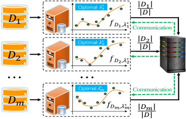
(a) Flow of training

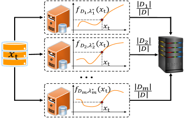
(b) Flow of testing

Figure 1: Training and testing flows of DKRR

Distributed learning (Balcan et al., 2012; Lea and Nicoll, 2013) is a promising approach for addressing the data silos, as it enables multiple parties to collaborate and learn from each other’s data without having to share the data themselves. As shown in Figure 1, there are generally three ingredients in a distributed learning scheme. The first one is local processing, in which each local machine (party) runs a specific learning algorithm with its own algorithmic parameters and data to yield a local estimator. The second one is communication, where several useful but non-sensitive pieces of information are communicated with each other to improve the quality of local estimators. To protect data privacy, neither data nor information that could lead to data disclosure is permitted to be communicated. The last one is synthesization, in which all local estimators are communicated to the global machine to synthesize a global estimator. In this way, multiple parties can collaborate on solving problems that require access to the whole data from different sources while also addressing privacy concerns, as sensitive data are kept in their original locations and only non-sensitive information is shared among the parties involved.

Due to the success in circumventing the data silos, numerous distributed learning schemes with solid theoretical verification have been developed, including distributed linear regression (Zhang et al., 2013), distributed online learning (Dekel et al., 2012), distributed conditional maximum entropy learning (Mcdonald et al., 2009), distributed kernel ridge regression (Zhang et al., 2015), distributed local average regression (Chang et al., 2017a), distributed kernel-based gradient descent (Lin and Zhou, 2018), distributed spectral algorithms (Mücke and Blanchard, 2018), distributed multi-penalty regularization algorithms (Guo et al., 2019), and distributed coefficient regularization algorithms (Shi, 2019). In particular, these algorithms have been proven to achieve optimal rates of generalization error bounds for their batch counterparts, as long as the algorithm parameters are properly selected and the number of local machines is not too large. However, how to choose appropriate algorithm parameters without sharing the data to achieve the theoretically optimal generalization performance of these distributed learning schemes is still open, because all the existing provable parameter selection strategies, such as the logarithmic mechanism for cross-validation (Liu et al., 2022), generalized cross-validation (Xu et al., 2019), and the discrepancy principle (Celisse and Wahl, 2021), need to access the whole data. This naturally raises the following problem:

Problem 1

How to develop a feasible parameter selection strategy without communicating the individual data of local machines with each other to equip distributed learning to realize its theoretically optimal generalization performance and successfully circumvent the data silos?

In this paper, taking distributed kernel ridge regression as an example, we develop an adaptive parameter selection strategy based on communicating non-sensitive information to solve the above problem. Our basic idea is to find a fixed basis, and each local machine computes an approximation of its derived rule (the relationship between the input and output) based on the basis and transfers the coefficients of the basis to the global machine. The global machine then synthesizes all the collected coefficients through a specific synthesis scheme and communicates the synthesized coefficients back to each local machine. In this way, each local machine obtains a good approximation of the global rule and uses this rule for cross-validation to determine its algorithm parameters. The road map of our approach is shown in Figure 2. Using the developed parameter selection strategy, we propose a novel adaptive distributed kernel ridge regression (AdaDKRR) to address the data silos. Our main contributions can be concluded as follows:

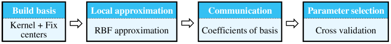
Figure 2: Road map of the proposed parameter selection strategy

$\bullet$ Methodology novelty: Since data stored in different local machines cannot be communicated, developing an adaptive parameter selection strategy based on local data to equip distributed learning is not easy. The main novelty of our approach is a nonparametric-to-parametric model transition method, which determines the algorithm parameters of distributed nonparametric learning schemes by communicating the coefficients of fixed basis functions without leaking any sensitive information about the local data. With such a novel design, we develop a provable and effective parameter selection strategy for distributed learning based on cross-validation to solve the data silos. As far as we know, this is the first attempt at designing provable parameter selection strategies for distributed learning to address the data silos.

$\bullet$ Theoretical assessments: Previous theoretical research (Zhang et al., 2015; Lin et al., 2017; Mücke and Blanchard, 2018; Shi, 2019) on distributed learning was carried out with three crucial assumptions: 1) the sizes of data in local machines are almost the same; 2) the parameters selected by different local machines are almost the same; 3) the number of local machines is not so large. In this paper, we present a detailed theoretical analysis by considering the role of the synthesization strategy and removing the assumption of the same data size. Furthermore, we borrow the idea of low-discrepancy sequences (Dick and Pillichshammer, 2010) and the classical radial basis function approximation (Wendland and Rieger, 2005; Rudi et al., 2015) to prove the feasibility of the proposed parameter selection strategy and remove the above-mentioned same parameter assumption. Finally, we provide an optimal generalization rate for AdaDKRR in the framework of statistical learning theory (Cucker and Zhou, 2007; Steinwart and Christmann, 2008), which shows that if the number of local machines is not so large, the performance of AdaDKRR is similar to running KRR on the whole data. This provides a solid theoretical verification for the feasibility of AdaDKRR to address the data silos.

$\bullet$ Experimental verification: We conduct both toy simulations and real-world data experiments to illustrate the excellent performance of AdaDKRR and verify our theoretical assertions. The numerical results show that AdaDKRR is robust to the number of basis functions, which makes the selection of the basis functions easy, thus obtaining satisfactory results. In addition, AdaDKRR shows stable and effective learning performances in parameter selection for distributed learning, regardless of whether the numbers of samples allocated to local machines are the same or not. We also apply AdaDKRR to two real-world data sets, including ones designed to help determine car prices and GPU acceleration models, to test its usability in practice.

The rest of this paper is organized as follows. In the next section, we introduce the challenges, motivations, and some related work of parameter selection in distributed learning. In Section 3, we propose AdaDKRR and introduce some related properties. In Section 4, we provide theoretical evidence of the effectiveness of the proposed adaptive parameter selection strategy and present an optimal generalization error bound for AdaDKRR. In Section 5, we numerically analyze the learning performance of AdaDKRR in toy simulations and two real-world applications. Finally, we draw a simple conclusion. The proofs of all theoretical results and some other relevant information about AdaDKRR are postponed to the Appendix.

2 Challenges, Our approaches, and Related Work

Let $({\mathcal{H}}_{K},\|\cdot\|_{K})$ be a reproducing kernel Hilbert space (RKHS) induced by a Mercer kernel $K$ (Cucker and Zhou, 2007) on a compact input space ${\mathcal{X}}$. Suppose there is a data set $D_{j}=\{(x_{i,j},y_{i,j})\}_{i=1}^{|D_{j}|}\subset\mathcal{X}\times\mathcal{Y}$ stored in the $j$-th local machine with $1\leq j\leq m$ and $\mathcal{Y}\subseteq\mathbb{R}$ as the output space. Without loss of generality, we assume that there are no common samples of local machines, i.e. $D_{j}\cap D_{j^{\prime}}=\varnothing$ for $j\neq j^{\prime}$. Distributed kernel ridge regression (DKRR) with regularization parameters $\vec{\lambda}:=\{\lambda_{1},\dots,\lambda_{m}\}$ is defined by (Zhang et al., 2015; Lin et al., 2017)

$$\overline{f}_{D,\vec{\lambda}}=\sum_{j=1}^{m}\frac{|D_{j}|}{|D|}f_{D_{j},\lambda_{j}},$$ (1)

where $\lambda_{j}>0$ is a regularization parameter for $j=1,\dots,m$, $D=\cup_{j=1}^{m}D_{j}$, $|D|$ denotes the cardinality of the data set $D$, and the local estimator $f_{D_{j},\lambda_{j}}$ is defined by

$$f_{D_{j},\lambda_{j}}=\arg\min_{f\in\mathcal{H}_{K}}\left\{\frac{1}{|D_{j}|}\sum_{(x,y)\in D_{j}}(f(x)-y)^{2}+\lambda_{j}\|f\|^{2}_{K}\right\}.$$ (2)

Therefore, in DKRR defined by (1), each local machine runs KRR (2) on its own data $D_{j}$ with a specific regularization parameter $\lambda_{j}$ to generate a local estimator, and the global machine synthesizes the global estimator $\overline{f}_{D,\vec{\lambda}}$ by using a weighted average based on data sizes. If $\lambda_{j}$ is given, then it does not need additional communications in DKRR to handle the data silos. However, how to choose $\lambda_{j}$ to optimize DKRR is important and difficult, as data are distributively stored across different local machines and cannot be shared.

2.1 Challenges and road-map for parameter selection in distributed learning

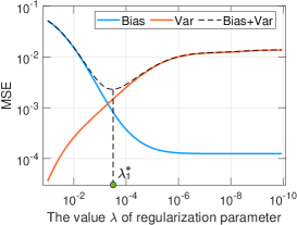
(a) DKRR-machine 1

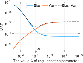
(b) DKRR

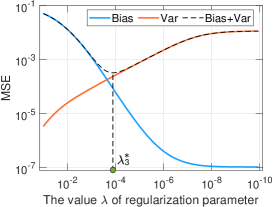
(c) KRR

Figure 3: Relationship between bias (variance) and regularization parameter values. Training data $\{(x_{i},y_{i})\}_{i=1}^{5000}$ are generated by drawing $\{x_{i}\}_{i=1}^{5000}$ i.i.d. according to the uniform distribution on $[0,1]^{3}$ and $y_{i}=g_{1}(x_{i})+\varepsilon$, where $g_{1}(x)$ is defined by (22) and $\varepsilon\sim\mathcal{N}(0,0.1^{2})$; testing data $\{(x_{i}^{\prime},y_{i}^{\prime})\}_{i=1}^{1000}$ are generated similarly to the training data but with a promise that $y_{i}^{\prime}=g_{1}(x_{i}^{\prime})$. The training samples are uniformly distributed to $m$ local machines, and the number $m$ is set to 10. “DKRR-machine1” represents running KRR on a local machine with a data subset of size $5000/m$.

Recalling that the introduction of the regularization term in (2) is to avoid the well-known over-fitting phenomenon (Cucker and Zhou, 2007) that the derived estimator fits the training data well but fails to predict other queries, the optimal regularization parameter is frequently selected when the bias is close to the variance. However, as shown in Figure 3, if we choose the theoretically optimal regularization parameter based on its own data in each local machine, it is usually larger than the optimal parameter of the global estimator, i.e., $\lambda_{1}^{*}>\lambda_{2}^{*}\sim\lambda_{3}^{*}$, resulting in the derived global estimator under-fitting. This is not surprising, as the weighted average in the definition of (1) helps to reduce the variance but has little influence on the bias, just as Figure 4 purports to show.

Therefore, a smaller regularization parameter than the theoretically optimal one is required for each local machine based on its own data, leading to over-fitting for each local estimator. The weighted average in (1) then succeeds in reducing the variance of DKRR and avoids over-fitting. The problem is, however, that each local machine only accesses its own data, making it difficult to determine the extent of over-fitting needed to optimize the performance of distributed learning. This refers to the over-fitting problem of parameter selection in distributed learning, and it is also the main challenge of our study.

(a) Bias

(b) Variance

Figure 4: Comparisons of bias and variance with different regularization parameter values. The data and simulation settings are the same as in Figure 3.

Generally speaking, there are two ways to settle the over-fitting problem of parameter selection in distributed learning. One is to modify the existing parameter selection strategies, such as cross-validation (Györfi et al., 2002; Caponnetto and Yao, 2010), the balancing principle (De Vito et al., 2010; Lu et al., 2020), the discrepancy principle (Raskutti et al., 2014; Celisse and Wahl, 2021), and the Lepskii principle (Blanchard et al., 2019), to force the local estimator in each local machine to over-fit their own data. A typical example is the logarithmic mechanism (Liu et al., 2022), which uses $\lambda_{j}^{\log_{|D_{j}|}|D|}$ to reduce the regularization parameter $\lambda_{j}$ selected by $D_{j}$ alone as the optimal one. Recalling that it is unknown what the extent of over-fitting should be, it is difficult for this approach to get appropriate regularization parameters to achieve the theoretically optimal learning performance established in (Zhang et al., 2015; Lin et al., 2017) of DKRR. The other is to modify the target functions for parameter selection in each local machine so that the existing strategies can directly find the optimal regularization parameter for distributed learning. We adopt the latter in this paper since it is feasible for this purpose by designing delicate communication strategies. In particular, it is possible to find a good approximation of the global estimator $\overline{f}_{D,\vec{\lambda}}$ by communicating non-private information.

Our approach is motivated by four interesting observations. First, it can be seen in Figure 3 that the optimal regularization parameter for the local estimator $f_{D_{j}}$ is not the optimal one for the global estimator. If we can find an approximation of the global estimator $\overline{f}_{D,\vec{\lambda}}$ and use this approximation instead of the local estimator $f_{D_{j},\lambda_{j}}$ as the target of parameter selection in the $j$-th local machine, then it is not difficult to determine a nearly optimal regularization parameter for the global estimator $\overline{f}_{D,\vec{\lambda}}$ through the existing parameter selection strategies. Second, due to privacy, it is impossible to communicate the local estimator $f_{D_{j},\lambda_{j}}$ directly since such a communication requires not only the coefficients of linear combinations of shifts of kernels but also the centers of the kernel that should be inputs of data $D_{j}$. However, these local estimators can be well approximated by linear combinations of some fixed basis functions, which is a classical research topic in approximation theory (Narcowich and Ward, 2004; Wendland and Rieger, 2005; Narcowich et al., 2006). Third, the well-developed sampling approaches including Monte Carlo sampling and Quasi-Monte Carlo sampling (Dick and Pillichshammer, 2010; Leobacher and Pillichshammer, 2014) introduced several low-discrepancy sequences, such as Sobol sequences, Niederreiter sequences, and Halton sequences, to improve the efficiency of the above approximation. Based on this, each local machine can generate the same centers of the kernel to establish a set of fixed basis functions, thus realizing the communication of functions by transmitting coefficients. Finally, though data cannot be communicated, some other non-private information, such as predicted values of queries, gradients, and coefficients of some basis functions, is communicable in distributed learning (Li et al., 2014; Lee et al., 2017; Jordan et al., 2019). According to the above four important observations, we design the road map for parameter selection in distributed learning, as shown in Figure 2.

As stated above, there are five crucial ingredients in our approach: basis functions generation, local approximation, communications, global approximation, and local parameter selection. For the first issue, we focus on searching low-discrepancy sequences (Dick and Pillichshammer, 2010; Leobacher and Pillichshammer, 2014) to form the centers of the kernel and then obtain a linear space spanned by these basis functions. For the second issue, we use the radial basis function approximation approach (Narcowich and Ward, 2004; Narcowich et al., 2006; Rudi et al., 2015) with the noise-free data $\left\{\left(x_{i,j},f_{D_{j},\lambda_{j}}(x_{i,j})\right)\right\}$ to provide a local approximation of the local estimator. For the third issue, each local machine transmits the coefficients of its local approximation to the global machine without leaking any sensitive information about its own data. For the fourth issue, the global machine synthesizes these coefficients by weighted average like (1) and transmits the synthesized coefficients back to all local machines. For the last issue, each local machine executes a specific parameter selection strategy to determine the regularization parameter of the global approximation. Noting that besides the coefficients of some fixed basis functions, the sensitive information of the data in local machines is not communicated, which implies that the proposed approach provides a feasible scheme to settle the data silos.

2.2 Related work

Since data silos caused by a combination of data privacy and interoperability impede the effective integration and management of data, it is highly desirable to develop feasible machine learning schemes to settle them and sufficiently explore the value of big data. Federated learning (Li et al., 2020) is a popular approach to handling the data silos. It starts with a pre-training model that all data holders know and aims at collaborative training through multiple rounds of communications of non-sensitive information from the data holders to aggregate a golden model. Although it has been numerically verified that federated learning is excellent in some specific application areas (Tuor et al., 2021; Li et al., 2022), the exploration of pre-training models and multiple rounds of communications leads to essential weaknesses of the current defense against privacy attacks, such as data poisoning, model poisoning, and inference attacks (Li et al., 2020; Lyu et al., 2020). More importantly, the lack of solid theoretical verifications restricts the use of federated learning in high-risk areas such as natural disaster prediction, financial market prediction, medical diagnosis prediction, and crime prediction.

Theoretically, nonparametric distributed learning based on a divide-and-conquer strategy (Zhang et al., 2015; Zhou and Tang, 2020) is a more promising approach for addressing the data silos. As shown in Figure 1, it does not need a pre-training model or multiple rounds of communications. Furthermore, solid theoretical verification has been established for numerous distributed learning schemes, including DKRR (Zhang et al., 2015; Lin et al., 2017), distributed gradient descents (Lin and Zhou, 2018), and distributed spectral algorithms (Guo et al., 2017a; Mücke and Blanchard, 2018), in the sense that such a distributed learning scheme performs almost the same as running the corresponding algorithms on the whole data under some conditions. These interesting results seem to show that distributed learning can successfully address the data silos while realizing the benefits of big data without communicating sensitive information about the data. However, all these exciting theoretical results are based on the assumption of proper selection of the algorithm (hyper-)parameters for distributed learning, which is challenging in reality if the data cannot be shared. This is the main reason why nonparametric distributed learning has not been practically used for settling the data silos, though its design flow is very suitable for this purpose.

As an open question in numerous papers (Zhang et al., 2015; Lin et al., 2017; Mücke and Blanchard, 2018; Zhao et al., 2019), the parameter selection of distributed learning has already been noticed by (Xu et al., 2019) and (Liu et al., 2022). In particular, Xu et al. (2019) proposed a distributed generalized cross-validation (DGCV) for DKRR and provided some solid theoretical analysis. It should be noted that the proposed DGCV essentially requires the communication of data, making it suffer from the data silos. Liu et al. (2022) proposed a logarithmic mechanism to force the over-fitting of local estimators without communicating sensitive information about local data and theoretically analyzed the efficacy of the logarithmic mechanism. However, their theoretical results are based on the assumption that the optimal parameter is algebraic with respect to the data size, which is difficult to verify in practice.

Compared with all these related works, our main novelty is to propose an adaptive parameter selection strategy to equip non-parametric distributed learning schemes and thus settle the data silos. It should be highlighted that our proposed approach only needs two rounds of communications of non-sensitive information. We provide the optimality guarantee in theory and the feasibility evidence in applications.

3 Adaptive Distributed Kernel Ridge Regression

In this section, we propose an adaptive parameter selection strategy for distributed kernel ridge regression, which is named AdaDKRR, to address the data silos. As discussed in the

  Algorithm 1  AdaDKRR with hold-out

 

1: Input: Training data subset $D_{j}=\{(x_{ij},y_{ij})\}_{i=1}^{|D_{j}|}$ with $x_{ij}\in\mathcal{X}$ and $|y_{ij}|\leq M$ stored in the $j$-th local machine for $j=1,\cdots,m$, a candidate set of the regularization parameter $\Lambda=\{\lambda_{\ell}\}_{\ell=1}^{L}$, and a query point $x$. Divide $D_{j}=\{(x_{ij},y_{ij})\}_{i=1}^{|D_{j}|}$ into training and validation sets, and denote them as $D_{j}^{tr}$ and $D_{j}^{val}$, respectively.

2:Local machines: given $\lambda_{\ell}\in\Lambda$ and $j$, run KRR with data $D_{j}^{tr}$ to obtain a local estimator

$$f_{D_{j}^{tr},\lambda_{\ell}}=\arg\min_{f\in\mathcal{H}_{K}}\left\{\frac{1}{|D_{j}^{tr}|}\sum_{(x,y)\in D_{j}^{tr}}(f(x)-y)^{2}+\lambda_{\ell}\|f\|^{2}_{K}\right\}.$$ (3)

$\triangleright$ Local Processing

3:Local machines: generate the same set of centers $\Xi_{n}=\{\xi_{k}\}_{k=1}^{n}$ and define a set of basis functions $B_{n,K}:=\left\{\sum_{k=1}^{n}a_{k}K_{\xi_{k}}:a_{k}\in\mathbb{R}\right\}$ with $K_{\xi}(x)=K(\xi,x)$. $\triangleright$ Basis Generation

4:Local machines: for some $s\in\mathbb{N}$, generate a set of points $\{x_{i,j}^{*}\}_{i=1}^{s}\subseteq\mathcal{X}$ and define an approximation of $f_{D_{j}^{tr},\lambda_{\ell}}$ by running KRR on data $\left\{\left(x_{i,j}^{*},f_{D_{j}^{tr},\lambda_{\ell}}(x^{*}_{i,j})\right)\right\}_{i=1}^{s}$, that is,

$${f}^{local}_{D_{j}^{tr},\lambda_{\ell},n,\mu,s}=\arg\min_{f\in B_{n,K}}\frac{1}{s}\sum_{i=1}^{s}\left(f(x^{*}_{i,j})-f_{D_{j}^{tr},\lambda_{\ell}}(x^{*}_{i,j})\right)^{2}+\mu\|f\|_{K}^{2}$$ (4)

for some $\mu>0$, and denote ${f}^{local}_{D_{j}^{tr},\lambda_{\ell},n,\mu,s}=\sum_{k=1}^{n}a^{local}_{j,k,\ell}K_{\xi_{k}}.$ $\triangleright$ Local Approximation

5:Local machines: transmit the cofficient matrix $\left(a^{local}_{j,k,\ell}\right)_{k=1,\ell=1}^{n,L}$ to the global machine.

6:$\triangleright$ Communication(I)

7:Global machine: synthesize the coefficients by ${a}^{global}_{k,\ell}=\sum_{j=1}^{m}\frac{|D^{tr}_{j}|}{|D^{tr}|}a^{local}_{j,k,\ell}$ and communicate $\left(a_{k,\ell}^{global}\right)_{k=1,\ell=1}^{n,L}$ to each local machine. $\triangleright$ Synthesization and Communication(II)

8:Local machines: obtain a global approximation ${f}^{global}_{D^{tr},{\lambda}_{\ell},n,\mu,s}$ as

$${f}^{global}_{D^{tr},{\lambda}_{\ell},n,\mu,s}:=\sum_{k=1}^{n}{a}^{global}_{k,\ell}K_{\xi_{k}}=\sum_{j=1}^{m}\frac{|D_{j}^{tr}|}{|D^{tr}|}\sum_{k=1}^{n}a^{local}_{j,k,\ell}K_{\xi_{k}}=\sum_{j=1}^{m}\frac{|D_{j}^{tr}|}{|D^{tr}|}{f}^{local}_{D_{j}^{tr},\lambda_{\ell},n,\mu,s}$$ (5)

and define

$$\lambda_{j}^{*}=\arg\min_{\lambda_{\ell}\in\Lambda}\frac{1}{|D_{j}^{val}|}\sum_{(x,y)\in D_{j}^{val}}\left(\pi_{M}{f}^{global}_{D^{tr},{\lambda}_{\ell},n,\mu,s}(x)-y\right)^{2}$$ (6)

with $\pi_{M}f(x)=\mbox{sign}(f(x))\min\{|f(x)|,M\}.$$\triangleright$ Local Validation

9:Local machines: calculate $\pi_{M}{f}^{global}_{D^{tr},\lambda^{*}_{j},n,\mu,s}(x)$ and communicate it to the global machine.

10:$\triangleright$ Communication(III)

11:Global machine: synthesize the AdaDKRR estimator as $\triangleright$ Global Estimator

$$\overline{f}^{Ada}_{D,\vec{\lambda}^{*}}(x):=\overline{f}^{Ada}_{D,\vec{\lambda}^{*},n,\mu,s}(x)=\sum_{j=1}^{m}\frac{|D_{j}|}{|D|}\pi_{M}{f}^{global}_{D^{tr},\lambda^{*}_{j},n,\mu,s}(x).$$ (7)

12: Output: The global estimator $\overline{f}^{Ada}_{D,\vec{\lambda}^{*}}(x)$.

 

previous section, our approach includes five important ingredients: basis generation, local approximation, communications, global approximation, and parameter selection. To ease the description, we use the “hold-out” approach (Caponnetto and Yao, 2010) in each local machine to adaptively select the parameter, though our approach can be easily designed for other strategies. The detailed implementation of AdaDKRR is shown in Algorithm 3.

Compared with the classical DKRR (Zhang et al., 2015; Lin et al., 2017), AdaDKRR presented in Algorithm 3 requires five additional steps (Steps 2–6) that include basis generation, local approximation, global approximation, and two rounds of communications with $\mathcal{O}(mnL)$ communication complexity. Algorithm 3 actually presents a feasible framework for selecting parameters of distributed learning, as the basis functions, local approximation, and global approximation are not unique. It should be highlighted that Algorithm 3 uses the “hold-out” method in selecting the parameters, while our approach is also available for cross-validation (Györfi et al., 2002), which requires a random division of the training data $D_{j}$. We refer the readers to Algorithm Appendix A: Training and Testing Flows of AdaDKRR in the Appendix for the detailed training and testing flows of the cross-validation version of AdaDKRR.

In the basis generation step (Step 2), we generate the same set of basis functions in all local machines so that the local estimators defined in (3) can be well approximated by linear combinations of these basis functions. Noting that the local estimators are smooth and in $\mathcal{H}_{K}$, numerous basis functions, such as polynomials, splines, and kernels, can approximate them well from the viewpoint of approximation theory (Wendland and Rieger, 2005). Since we have already obtained a kernel $K$, we use the kernel to build up the basis functions, and then the problem boils down to selecting a suitable set of centers $\Xi_{n}:=\{\xi_{k}\}_{k=1}^{n}$ so that $\mbox{span}\{K_{\xi_{k}}\}$ can well approximate functions in $\mathcal{H}_{K}$. There are roughly two approaches to determining $\Xi_{n}$. One is to generate a set of fixed low sequences, such as Sobol sequences and Halton sequences, with the same size (Dick and Pillichshammer, 2010). It can be found in (Dick and Pillichshammer, 2010) that the complexity of generating $n$ Sobol sequences (or Halton sequences) is $\mathcal{O}(n\log n)$. Furthermore, it can be found in (Dick and Pillichshammer, 2010; Dick, 2011; Feng et al., 2021) that there are $c,\beta>0$ such that

$$\sup_{\|f\|_{K}\leq 1,\|g\|_{K}\leq 1}\left|\int f(x)g(x)dP_{u}(x)-\frac{1}{n}\sum_{k=1}^{n}f(\xi_{k})g(\xi_{k})\right|\leq cn^{-\beta},$$ (8)

where $P_{u}$ denotes a uniform distribution. The other method is to generate $n$ points (in a random manner according to a uniform distribution) in the global machine, and then the global machine transmits this set of points to all local machines. In this paper, we focus on the first method to reduce the cost of communications, though the second one is also feasible.

In the local approximation step (Step 3), we aim to finding a good approximation of the local estimator $f_{D_{j}^{tr},\lambda_{\ell}}$. The key is to select a suitable set of points $\{x_{i,j}^{*}\}_{j=1}^{s}$ and a suitable parameter $\mu$ so that the solution to (4) can well approximate $f_{D_{j}^{tr},\lambda_{\ell}}$. Since there are already two point sets, $\{x_{i,j}\}_{i=1}^{|D_{j}^{tr}|}$ and $\{\xi_{k}\}_{k=1}^{n}$, we can select one of them as $\{x_{i,j}^{*}\}_{j=1}^{s}$. In this paper, we use the former, but choosing the latter is also reasonable because the solution to (4) is a good approximation of the local estimator (Wendland and Rieger, 2005). Noting $s=|D_{j}^{tr}|$, we write $f^{local}_{D_{j}^{tr},\lambda_{\ell},n,\mu,s}$ as $f^{local}_{D_{j}^{tr},\lambda_{\ell},n,\mu}$. Recalling the idea of Nyström regularization (Rudi et al., 2015; Sun et al., 2021) and regarding (4) as a Nyström regularization scheme with the noise-free data $\left\{\left(x_{i,j},f_{D_{j}^{tr},\lambda_{\ell}}(x_{i,j})\right)\right\}_{i=1}^{|D_{j}^{tr}|}$, we obtain from (4) that ${f}^{local}_{D_{j}^{tr},\lambda_{\ell},n,\mu}(\cdot)=\sum_{k=1}^{n}\alpha^{local}_{j,k,\ell}K_{\xi_{k}}(\cdot),$ where

$$\vec{a}_{j,\ell}^{local}:=\left(a_{j,1,\ell}^{local},\cdots,a_{j,n,\ell}^{local}\right)^{T}=\left(\mathbb{K}_{\left|D_{j}^{tr}\right|,n}^{T}\mathbb{K}_{\left|D_{j}^{tr}\right|,n}+\mu\left|D_{j}^{tr}\right|\mathbb{K}_{n,n}\right)^{\dagger}\mathbb{K}_{\left|D_{j}^{tr}\right|,n}^{T}{\vec{f}}_{D_{j}^{tr},\lambda_{\ell}},$$ (9)

$A^{\dagger}$ and $A^{T}$ denote the Moore-Penrose pseudo-inverse and transpose of a matrix $A$, respectively, $\left(\mathbb{K}_{|D_{j}^{tr}|,n}\right)_{i,k}=K(x_{i,j},\xi_{k})$, $(\mathbb{K}_{n,n})_{k,k^{\prime}}=K(\xi_{k},\xi_{k^{\prime}})$, and $\vec{f}_{D_{j}^{tr},\lambda_{\ell}}=\left(f_{D_{j}^{tr},\lambda_{\ell}}(x_{1,j}),\dots,\right.$ $\left.f_{D_{j}^{tr},\lambda_{\ell}}(x_{\left|D_{j}^{tr}\right|,j})\right)^{T}$. Therefore, it requires $\mathcal{O}\left(|D_{j}^{tr}|n^{2}+n^{3}\right)$ floating computations to derive the local approximation. Since $\left\{\left(x_{i,j},f_{D_{j}^{tr},\lambda_{\ell}}(x_{i,j})\right)\right\}_{i=1}^{|D_{j}^{tr}|}$ is noise-free, the parameter $\mu$ in (4) is introduced to overcome the ill-conditionness of the linear least problems and thus can be set to be small (e.g., $\mu=10^{-4}$).

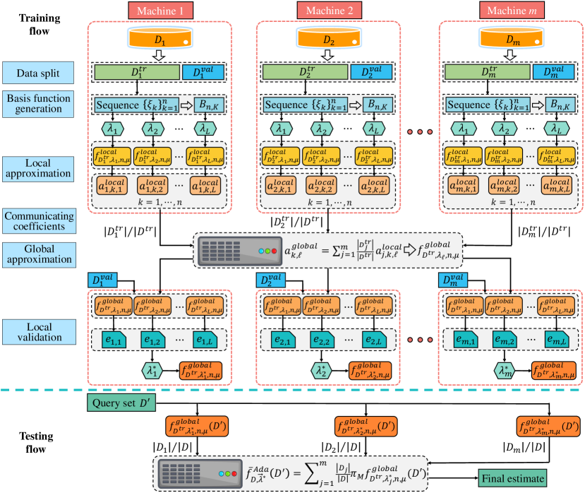
Figure 5: Training and testing flows of the proposed method

In the global approximation step (Step 6), the global approximation is obtained through a weighted average. The optimal parameters of local machines are then searched for the global approximation via the validation set. If $f^{local}_{D_{j}^{tr},\lambda_{\ell},n,\mu}$ is a good approximation of $f_{D_{j}^{tr},\lambda_{\ell}}$, then $f^{global}_{D^{tr},\lambda_{\ell},n,\mu}$ is a good approximation of the global estimator $\overline{f}_{D^{tr},\lambda_{\ell}}$ defined by (1). Therefore, the optimal parameters selected for the global approximation are close to those of the global estimator. It should be noted that introducing the truncation operator $\pi_{M}$ in parameter selection is to ease the theoretical analysis and does not require additional computation. It requires $\mathcal{O}\left(|D_{j}^{val}|nL\right)$ floating computations in this step. The flows of AdaDKRR adopted in this paper can be found in Figure 5.

4 Theoretical Verifications

In this section, we study the generalization performance of AdaDKRR defined by (7) in a framework of statistical learning theory (Cucker and Zhou, 2007; Steinwart and Christmann, 2008), where samples in $D_{j}$ for $j=1,2,\dots,m$ are assumed to be independently and identically drawn according to an unknown joint distribution $\rho:=\rho(x,y)=\rho_{X}(x)\rho(y|x)$ with the marginal distribution $\rho_{X}$ and the conditional distribution $\rho(\cdot|x)$. The regression function $f_{\rho}(x)=E[y|X=x]$ minimizes the generalization error $\mathcal{E}(f):=\int_{\mathcal{Z}}(f(x)-y)^{2}d\rho$ for $f\in L_{\rho_{X}}^{2}$, where $L^{2}_{\rho_{{}_{X}}}$ denotes the Hilbert space of $\rho_{X}$-square integrable functions on $\mathcal{X}$, with the norm denoted by $\|\cdot\|_{\rho}$. Therefore, the purpose of learning is to obtain an estimator $f_{D}$ based on $D_{j}$ for $j=1,2,\dots,m$ to approximate the regression function $f_{\rho}$ without leaking the privacy information of $D_{j}$. In this way, the performance of the global estimator $\overline{f}^{Ada}_{D,\vec{\lambda}^{*}}$ is quantitatively measured by the excess generalization error

$$\mathcal{E}(\overline{f}^{Ada}_{D,\vec{\lambda}^{*}})-\mathcal{E}(f_{\rho})=\left\|\overline{f}^{Ada}_{D,\vec{\lambda}^{*}}-f_{\rho}\right\|^{2}_{\rho},$$ (10)

which describes the relationship between the prediction error and the data size.

4.1 Generalization error for DKRR

Before presenting the generalization error analysis for AdaDKRR, we first study the theoretical assessments of DKRR, which have been made in (Zhang et al., 2015; Lin et al., 2017) to show that DKRR performs similarly to running KRR on the whole data stored in a large enough machine, provided $m$ is not so large, $|D_{1}|\sim\dots\sim|D_{j}|$, and the regularization parameters $\lambda_{1}\sim\dots\sim\lambda_{m}$ are similar to the optimal regularization parameter of KRR with the whole data.

The restriction on the number of local machines is natural since it is impossible to derive satisfactory generalization error bounds for DKRR when $m=|D|$, i.e., there is only one sample in each local machine. However, the assumptions $|D_{1}|\sim\dots\sim|D_{j}|$ and $\lambda_{1}\sim\dots\sim\lambda_{m}$ are a little bit unreasonable. On the one hand, local agents attending to the distributed learning system frequently have different data sizes, making it unrealistic to assume that the data sizes of local machines are the same. On the other hand, it is difficult to develop a parameter selection strategy for local machines so that $\lambda_{1}\sim\dots\sim\lambda_{m}$ are similar to the optimal regularization parameter of KRR with the whole data, as local agents only access their own data.

Noticing these, we derive optimal generalization error bounds for DKRR without the assumptions $|D_{1}|\sim\dots\sim|D_{j}|$ and $\lambda_{1}\sim\cdots\sim\lambda_{m}$ the same as the theoretically optimal one. For this purpose, we introduce several standard assumptions on the data $D_{j}$, regression function $f_{\rho}$, and kernel $K$. As shown in Algorithm 3, our first assumption is the boundedness assumption of the output.

Assumption 1

There exists a $M>0$ such that $|y|\leq M$ almost surely.

Assumption 1 is quite mild since we are always faced with finitely many data, whose outputs are naturally bounded. It should be mentioned that Assumption 1 implies $\|f_{\rho}\|_{L^{\infty}}\leq M$ directly. To present the second assumption, we should introduce the integral operator $L_{K}$ on ${\mathcal{H}}_{K}$ (or $L_{\rho_{X}}^{2}$) given by

$$L_{K}f:=\int_{\mathcal{X}}K_{x}f(x)d\rho_{X},\qquad f\in{\mathcal{H}}_{K}\quad(\mbox{or}\ f\in L_{\rho_{X}}^{2}).$$

The following assumption shows the regularity of the regression function $f_{\rho}$.

Assumption 2

For some $r>0$, assume

$$f_{\rho}=L_{K}^{r}h_{\rho},~{}~{}{\rm for~{}some}~{}h_{\rho}\in L_{\rho_{X}}^{2},$$ (11)

where $L_{K}^{r}$ denotes the $r$-th power of $L_{K}:L_{\rho_{X}}^{2}\to L_{\rho_{X}}^{2}$ as a compact and positive operator.

According to the no-free-lunch theory (Györfi et al., 2002, Chap.3), it is impossible to derive a satisfactory rate for the excess generalization error if there is no restriction on the regression functions. Assumption 2 actually connects $f_{\rho}$ with the adopted kernel $K$, where the index $r$ in (11) quantifies the relationship. Indeed, (11) with $r=1/2$ implies $f_{\rho}\in\mathcal{H}_{K}$, $0<r<1/2$ implies $f_{\rho}\notin\mathcal{H}_{K}$, and $r>1/2$ implies that $f_{\rho}$ is in an RKHS generated by a smoother kernel than $K$.

Our third assumption is on the property of the kernel, measured by the effective dimension (Caponnetto and De Vito, 2007),

$$\mathcal{N}(\lambda)={\rm Tr}((\lambda I+L_{K})^{-1}L_{K}),\qquad\lambda>0.$$

Assumption 3

There exists some $s\in(0,1]$ such that

$$\mathcal{N}(\lambda)\leq C_{0}\lambda^{-s},$$ (12)

where $C_{0}\geq 1$ is a constant independent of $\lambda$.

It is obvious that (12) always holds with $s=0$ and $C_{0}=\kappa:=\sqrt{\sup_{x\in\mathcal{X}}K(x,x)}$. As discussed in (Fischer and Steinwart, 2020), Assumption 3 is equivalent to the eigenvalue decay assumption employed in (Caponnetto and De Vito, 2007; Steinwart et al., 2009; Zhang et al., 2015). It quantifies the smoothness of the kernel and the structure of the marginal distribution $\rho_{X}$. For example, if $\rho_{X}$ is the uniform distribution on the unit cube in the $d$-dimensional space $\mathbb{R}^{d}$ (i.e., $\mathcal{X}=\mathbb{I}^{d}$), and $K$ is a Sobolev kernel of order $\tau>d/2$, then Assumption 3 holds with $s=\frac{d}{2\tau}$ (Steinwart et al., 2009). The above three assumptions have been widely used to analyze generalization errors for kernel-based learning algorithms (Blanchard and Krämer, 2016; Chang et al., 2017b; Dicker et al., 2017; Guo et al., 2017a, b; Lin et al., 2017; Lin and Zhou, 2018; Mücke and Blanchard, 2018; Shi, 2019; Fischer and Steinwart, 2020; Lin et al., 2020; Sun et al., 2021), and optimal rates of excess generalization error for numerous learning algorithms have been established under these assumptions.

Under these well-developed assumptions, we provide the following theorem that DKRR can achieve the optimal rate of excess generalization error established for KRR with the whole data (Caponnetto and De Vito, 2007; Lin et al., 2017; Fischer and Steinwart, 2020), even when different local machines possess different data sizes.

Theorem 1

Under Assumption 1, Assumption 2 with $\frac{1}{2}\leq r\leq 1$, and Assumption 3 with $0<s\leq 1$, if

$$\lambda_{j}=C_{1}\left\{\begin{array}[]{cc}|D|^{-\frac{1}{2r+s}},&\mbox{if}\quad|D_{j}|\geq|D|^{\frac{1}{2r+s}}\log^{4}|D|,\\ |D_{j}|^{-1}\log^{4}|D|,&\mbox{otherwise},\end{array}\right.$$ (15)

and

$$m\leq|D|^{\frac{s}{2r+s}}(\log|D|)^{-8r},$$ (16)

then

$$E\left[\|\overline{f}_{D,\vec{\lambda}}-f_{\rho}\|_{\rho}^{2}\right]\leq C_{2}|D|^{-\frac{2r}{2r+s}},$$ (17)

where $C_{1}$ and $C_{2}$ are constants independent of $|D|$ or $m$.

Under Assumptions 1–3, it can be found in (Caponnetto and De Vito, 2007) that the derived learning rates in (17) are optimal in the sense that there is a regression function $f^{*}_{\rho}$ satisfying the above three assumptions such that

$$E\left[\|\overline{f}_{D,\vec{\lambda}}-f_{\rho}^{*}\|_{\rho}^{2}\right]\geq C_{3}|D|^{-\frac{2r}{2r+s}}$$

for a constant $C_{3}$ depending only on $r$ and $s$. Unlike the existing results on distributed learning (Zhang et al., 2015; Lin et al., 2017; Mücke and Blanchard, 2018; Lin et al., 2020) that imposed strict restrictions on the data sizes of local machines, i.e., $|D_{1}|\sim|D_{2}|\sim\dots\sim|D_{m}|$, Theorem 1 removes this condition since it is difficult to guarantee the same data size for all participants in the distributed learning system. As a result, it requires completely different mechanisms (15) to select the regularization parameter and stricter restriction on the number of local machines (16). The main reason for the stricter restriction on $m$ is that the distributed learning system accommodates local machines with little data, i.e., $|D_{j}|\leq|D|^{\frac{1}{2r+s}}\log^{4}|D|$. If we impose a qualification requirement that each participant in the distributed learning system has at least $|D|^{\frac{1}{2r+s}}\log^{4}|D|$ samples, then the restriction can be greatly relaxed, just as the following corollary shows.

Corollary 2

Under Assumption 1, Assumption 2 with $\frac{1}{2}\leq r\leq 1$, and Assumption 3 with $0<s\leq 1$, if $|D_{j}|\geq|D|^{\frac{1}{2r+s}}\log^{4}|D|$, $\lambda_{j}=C_{1}|D|^{-\frac{1}{2r+s}}$ for all $j=1,2,\dots,m$, and

$$m\leq|D|^{\frac{2r+s-1}{2r+s}}\log^{-4}|D|,$$ (18)

then

$$E\left[\|\overline{f}_{D,\vec{\lambda}}-f_{\rho}\|_{\rho}^{2}\right]\leq C_{2}|D|^{-\frac{2r}{2r+s}},$$ (19)

where $C_{1}$ and $C_{2}$ are constants independent of $|D|$ or $m$.

Theorem 1 and Corollary 2 provide a baseline for the analysis of AdaDKRR in terms that the generalization error of AdaDKRR should be similar to (17).

4.2 Learning performance of AdaDKRR

In this subsection, we study the theoretical behavior of AdaDKRR (7) by estimating its generalization error in the following theorem.

Theorem 3

Under Assumption 1, Assumption 2 with $1/2\leq r\leq 1$, and Assumption 3 with $0<s\leq 1$, if $\rho_{X}$ is a uniform distribution, $|D_{j}|\geq(8C_{1}^{*}(\log(1+\kappa)+2))^{2}|D|^{\frac{1}{2r+s}}\log^{4}|D|$, $\Lambda$ contains a $\bar{\lambda}\sim|D|^{-\frac{1}{2r+s}}$, and

$$m\leq\min\left\{|D|^{\frac{2r+s-1}{4r+2s}}\log^{-4}|D|,|D|^{\frac{s}{2r+s}}\log^{-1}L\right\},$$ (20)

then for any $\mu\in\left[\left(8C_{1}^{*}\left(\log(1+\kappa)+2\right)\right)^{2}\max_{j=1,\dots,m}\frac{\log^{4}|D_{j}^{tr}|}{|D_{j}^{tr}|},|D|^{-\frac{1}{2r+s}}\right]$ and $\Xi_{n}$ satisfying (8) for some $c,\beta>0$ with $\mu n^{\beta}\geq 2c$, there holds

$$E\left[\left\|\overline{f}^{Ada}_{D,\vec{\lambda^{*}}}-f_{\rho}\right\|_{\rho}^{2}\right]\leq C|D|^{-\frac{2r}{2r+s}},$$ (21)

where $C,C_{1}^{*}$ are constants depending only on $\|h_{\rho}\|_{\rho},M,r,C_{0},c,$ and $\beta$.

Compared with Theorem 1, it can be found that AdaDKRR possesses the same generalization error bounds under some additional restrictions, implying that the proposed parameter selection strategy is optimal in the sense that no other strategies always perform better. There are five additional restrictions that may prohibit the wide use of the proposed approach: (I) $m$ satisfies (20); (II) $|D_{j}|\geq(8C_{1}^{*}(\log(1+\kappa)+2))^{2}|D|^{\frac{1}{2r+s}}\log^{4}|D|$; (III) $\Lambda$ contains a $\bar{\lambda}\sim|D|^{-\frac{1}{2r+s}}$; (IV) $\rho_{X}$ is a uniform distribution; (V) $\mu\in\left(\left(8C_{1}^{*}(\log(1+\kappa)+2)\right)^{2}\right.$ $\left.\max_{j=1,\dots,m}{(\log^{4}|D_{j}^{tr}|})/{|D_{j}^{tr}|},|D|^{-\frac{1}{2r+s}}\right)$ and $\Xi_{n}$ satisfies (8) for some $c,\beta>0$ with $n$ satisfying $\mu n^{\beta}\geq 2c$.

Condition (I) is necessary since it is impossible to derive a satisfactory distributed learning estimator when each local machine has only one sample. Condition (II) presents a qualification requirement for the local machines participating in the distributed learning system, indicating that their data sizes should not be so small. Condition (III) means that the candidate set $\Lambda$ should include the optimal parameter. Noting (20), the restriction on $m$ is logarithmic with respect to $L$, and we can set $\Lambda=\{\lambda_{k}\}_{k=1}^{L}$ with $\lambda_{k}=q^{k}$ for some $q\in(0,1)$ and $L\sim|D|$. Conditions (IV) and (V) are mainly due to setting $\{x_{i,j}^{*}\}_{i=1}^{s}$ to $\{x_{i,j}\}_{i=1}^{|D_{j}|}$ in the local approximation step (Step 3 in Algorithm 3). Therefore, we have to use the quadrature property (8) of the low-discrepancy property, which requires the samples to be drawn i.i.d. according to the uniform distribution. Furthermore, the well-conditioness of the local approximation imposes a lower bound of $\mu$. Since $|D_{j}|\geq(8C_{1}^{*}(\log(1+\kappa)+2))^{2}|D|^{\frac{1}{2r+s}}\log^{4}|D|$, it is easy to check that $(8C_{1}^{*}(\log(1+\kappa)+2))^{2}\frac{\log^{4}|D_{j}^{tr}|}{|D_{j}^{tr}|}\leq|D|^{-\frac{1}{2r+s}}$, and there are numerous feasible values for $\mu$. The restriction on $\mu$ is to theoretically verify the well-conditionness of the local approximation in the worst case. In practice, it can be set to $10^{-4}$ directly. It would also be interesting to set a suitable $\{x_{i,j}^{*}\}_{i=1}^{s}$ to remove or relax conditions (IV) and (V).

As shown in Theorem 3, under some assumptions, we prove that AdaDKRR performs similarly to running the optimal learning algorithms on the whole data $D=\cup_{j=1}^{m}D_{j}$ without considering data privacy. Recalling in Algorithm 3 that AdaDKRR only requires communicating non-sensitive information, it is thus a feasible strategy to address the data silos.

5 Experimental Results

In this section, we use the following parameter selection methods for distributed learning to conduct experiments on synthetic and real-world data sets:

• On each local machine, the parameters are selected by cross-validation, and DKRR is executed with these selected parameters; we call this method DKRR with cross-validation (“DKRR” for short).

• On the $j$-th local machine, we first select parameters by cross-validation, and then transform the selected regularization parameter $\lambda_{j}$ by $\lambda_{j}\leftarrow\lambda_{j}^{\log{|D|}/\log{|D_{j}|}}$, and transform the selected kernel width $\sigma_{j}$ by $\sigma_{j}\leftarrow\sigma_{j}^{\log{|D|}/\log{|D_{j}|}}$ if the Gaussian kernel is used; DKRR is executed with these transformed parameters; we call this method DKRR with cross-validation and logarithmic transformation (“DKRRLog” for short).

• The proposed adaptive parameter selection method is applied to distributed learning and is denoted by “AdaDKRR”.

All the experiments are run on a desktop workstation equipped with an Intel(R) Core(TM) i9-10980XE 3.00 GHz CPU, 128 GB of RAM, and Windows 10. The results are recorded by averaging the results from multiple individual trials with the best parameters.

5.1 Synthetic Results

In this part, the performance of the proposed method is verified by four simulations. The first one studies the influence of the number and type of center points for local approximation on generalization ability. The second one exhibits the robustness of AdaDKRR to the number of center points. The third simulation presents comparisons of the generalization ability of the three mentioned methods with changing the number of local machines, provided that all training samples are uniformly distributed to local machines. The last simulation focuses on comparisons of generalization ability for the three methods when the training samples are unevenly distributed on local machines.

Before carrying out experiments, we describe the generating process of the synthetic data and some important settings of the simulations. The inputs $\{x_{i}\}_{i=1}^{N}$ of training samples are independently drawn according to the uniform distribution on the (hyper-)cube $[0,1]^{d}$ with $d=3$ or $d=10$. The corresponding outputs $\{y_{i}\}_{i=1}^{N}$ are generated from the regression models $y_{i}=g_{j}(x_{i})+\varepsilon$ with the Gaussian noise $\mathcal{N}(0,0.2)$ for $j=1,2$, where

$$g_{1}(x)=\left\{\begin{array}[]{ll}(1-\|x\|_{2})^{6}(35\|x\|_{2}^{2}+18\|x\|_{2}+3)&\quad\mbox{if}~{}0<\|x\|_{2}\leq 1,\\ 0&\quad\mbox{if}~{}\|x\|_{2}>1,\end{array}\right.$$ (22)

for the 3-dimensional data, and

$$g_{2}(x)=\left(\|x\|_{2}-1\right)\left(\|x\|_{2}-2\right)\left(\|x\|_{2}-3\right)$$ (23)

for the 10-dimensional data. The generation of test sets $\{(x_{i}^{\prime},y_{i}^{\prime})\}_{i=1}^{N^{\prime}}$ is similar to that of training sets, but it has the promise of $y_{i}^{\prime}=g_{j}(x_{i}^{\prime})$.

For the 3-dimensional data, we use the kernel function $K_{1}(x_{1},x_{2})=h(\|x_{1}-x_{2}\|_{2})$ with

$$h(r)=\left\{\begin{array}[]{ll}(1-r)^{4}(4r+1)&\quad\mbox{if}~{}0<r\leq 1,\\ 0&\quad\mbox{if}~{}r>1,\end{array}\right.$$ (24)

and the regularization parameter $\lambda$ is chosen from the set $\{\frac{1}{2^{q}}|\frac{1}{2^{q}}\geq 10^{-10},q=0,1,2,\cdots\}$. For the 10-dimensional data, we use the Gaussian kernel $K_{2}(x_{1},x_{2})=\exp\left(-\frac{\|x_{1}-x_{2}\|_{2}^{2}}{2\sigma^{2}}\right)$, the regularization parameter $\lambda$ is chosen from the set $\{\frac{1}{3^{q}}|\frac{1}{3^{q}}\geq 10^{-10},q=0,1,2,\cdots\}$, and the kernel width $\sigma$ is chosen from 10 values that are drawn in a logarithmic, equally spaced interval $[0.1,10]$. In the simulations, we generate $10000$ samples for training and $1000$ samples for testing, and the regularization parameter $\mu$ for local approximation is fixed as $10^{-4}$.

Dim=3

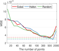
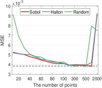
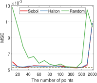
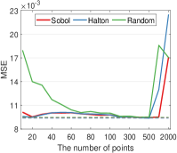
Dim=10

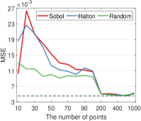
(a) $m=20$

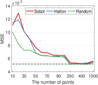
(b) $m=40$

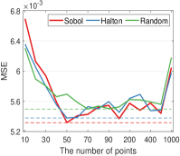
(c) $m=80$

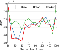
(d) $m=160$

Figure 6: Relationship between test MSE and the number of center points in local approximation using the three low-discrepancy sequences for AdaDKRR with different numbers of local machines

Simulation 1: In this simulation, we select three types of center points for local approximation, including two QMCS (Sobol points and Halton points) and one MCS (random points). The number $m$ of local machines varies from the set $\{20,40,80,160\}$. For each fixed $m$, the relation between the test MSE and the number $n$ of center points is shown in Figure 6, in which the dashed lines exhibit the best test MSEs with the optimal numbers of the three types of center points. From the above results, we have the following observations: 1) As the number of center points increases, the curves of test MSE have a trend of descending first and then ascending. This is because very few center points cannot provide satisfactory accuracy for local approximation, resulting in the approximate function based on the center points having a large deviation from the ground truth, while a large number of center points put the estimator at risk of over-fitting. 2) The optimal number of center points generally decreases as the number of local machines increases. Because a smaller $m$ indicates that there are more training samples on each local machine, more center points are required to cover these samples to obtain a satisfactory local approximation. 3) The three types of center points perform similarly on the 3-dimensional data, but Sobol points and Halton points are obviously better than random points on the 10-dimensional data, especially for larger numbers of local machines. In addition, the optimal number of random points is usually larger than the number of Sobol points and Halton points. The reason is that the discrepancy of QMCS is smaller than that of MCS, indicating that the sample distribution of QMCS is more uniform than that of MCS. Therefore, QMCS can better describe the structural information of the data and is more effective than MCS in local approximation. Since Sobol points perform similarly to Halton points, we take Sobol points as an example to demonstrate the superiority of the proposed method in the following experiments.

Simulation 2: In this simulation, we check the robustness of the proposed method concerning the number $n$ of center points, as $n$ determines the accuracy of the local approximation. We set the number $n$ in two ways: 1) by fixing $n$ as a constant (denoted by “$n=\#$”), and 2) by adaptively adjusting $n$ as the average number of training samples in each local machine (denoted by “$n=|D|/m$”). We vary the number of Sobol points from the sets $\{10,20,\cdots,100,200,\cdots,500,1000,2000\}$ and $\{10,20,\cdots,100,200,\cdots,500,1000\}$ for the 3-dimensional and 10-dimensional data, respectively, and vary the number of local machines from the set $\{20,40,80,150,300\}$. The testing RMSEs with respect to different orders of magnitude $n$ under different numbers of local machines are shown in Figure 7, where “$n$ best” represents the optimal MSE corresponding to the best $n$ chosen from the candidate set and provides a baseline for assessing the performance of the proposed method. From the results, it can be seen that the generalization performances with different orders of $n$ are all comparable with the best $n$ when $m$ is large (e.g., $m\geq 80$). Even when $m$ is small, we can also obtain a satisfactory result by simply varying a few different orders of magnitude of $n$. In addition, for different numbers of local machines, the proposed method with an adaptive number of center points shows stable performance that is comparable to the best $n$. All these results demonstrate that the proposed method is robust to the number of center points.

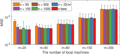
(a) Dim=3

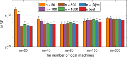
(b) Dim=10

Figure 7: Relationship between test MSE and the number of Sobol points for AdaDKRR with different numbers of local machines

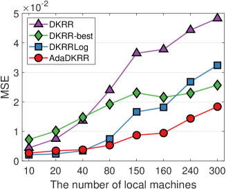
(a) Dim=3

(b) Dim=10

Figure 8: Comparisons of test MSE among the three parameter selection approaches with different numbers of local machines

Simulation 3: This simulation compares the proposed method with DKRR and DKRRLog under the condition that all training samples are uniformly distributed to local machines. The number of local machines changes from the set $\{10,20,40,80,150,160,240,300\}$. For AdaDKRR, the number $n$ of Sobol points is chosen from the set $\{50,100,500,1000\}$. The results of test MSE as a function of the number of local machines are shown in Figure 8, where “DKRR-best” denotes the best performance of local machines in DKRR. Based on the above results, we have the following observations: 1) The test MSE grows as the number of local machines increases for all methods, but the growth of AdaDKRR is much slower than that of other methods. 2) When the number of local machines is small (e.g., $m\leq 40$), DKRR-best has the worst performance; the MSE values of DKRR are smaller than those of DKRR-best, which verifies that distributed learning can fuse the information of local machines and achieve better generalization performance than each local machine; AdaDKRR performs similarly to DKRRLog, and both of them are significantly better than DKRR, which provides evidence that it is not a good choice to select parameters only based on the data in each local machine. 3) When the number of local machines increases, the generalization performance of DKRR and DKRRLog deteriorates dramatically, even worse than that of a single local machine (e.g., $m\geq 200$), whereas the test MSE of AdaDKRR grows slowly and has obvious superiority to other methods. These results show that the proposed method is effective and stable in parameter selection for distributed learning.

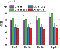
(a) $m=40$

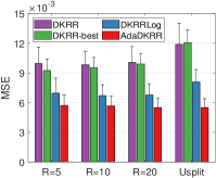
(b) $m=80$

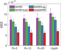
(c) $m=150$

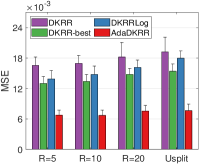
(d) $m=300$

Figure 9: Comparisons of test MSE among the three parameter selection approaches with different distribution patterns of data in local machines

Simulation 4: In this simulation, we compare the generalization performance of the three methods under non-uniform distributions of the number of training samples in local machines. Specifically, all training samples are randomly distributed to local machines, meaning the numbers of training samples in local machines are also random. In addition, we set the minimum number of training samples on each local machine so that cross-validation could be performed. For example, “$R=5$” means that the minimum number of training samples on each local machine is no less than 5. AdaDKRR uses the adaptive number of Sobol points (i.e., $n=|D|/m$) in local approximation for convenience. The number $m$ of local machines varies from the set $\{40,80,150,300\}$. For each fixed number $m$, we compare the generalization performance in four cases, including $R\in\{5,10,20\}$ and uniform split (denoted as “Usplit”), and the results are shown in Figure 9. Note that the case “Usplit” can be considered as “$R=|D|/m$”. From the results, we can see that the performance differences among the three methods in each case of the non-uniform split are similar to those in the case of the uniform split, as described in Simulation 3. Additionally, the test MSE usually increases from the case “$R=5$ to the case “Usplit”. This is because a smaller value of $R$ means that the distribution of the number of samples is more uneven, and the generalization performance of a single local machine with a large number of training samples is much better than that of a combination of several local machines with the same total number of training samples, as distributed learning shows. Compared with DKRR and DKRRLog, AdaDKRR is more robust to the split of training samples distributed to local machines, especially for the 10-dimensional data. The above results demonstrate that AdaDKRR is suitable for distributed learning with different data sizes of participants.

5.2 Real-World Applications

The mentioned parameter selection methods are tested on two real-world data sets: used car price forecasting and graphics processing unit (GPU) performance prediction for single-precision general matrix multiplication (SGEMM). Before discussing the experiments, it is important to clarify some implementation details: 1) For each data set, half of the data samples are randomly chosen as training samples, and the other half are used as testing samples to evaluate the performance of the mentioned methods. Following the typical evaluation procedure, 10 independent sets of training and testing samples are generated by running 10 random divisions on the data set. 2) For each data set, min-max normalization is performed for each attribute except the target attribute. Specifically, the minimum and maximum values of the $i$-th attribute of training samples are calculated and denoted by $F_{min}^{(i)}$ and $F_{max}^{(i)}$, respectively. The $i$-th attribute of samples is rescaled using the formula $\hat{\mathbf{x}}_{i}=\left(\mathbf{x}_{i}-F_{min}^{(i)}\right)/\left(F_{max}^{(i)}-F_{min}^{(i)}\right)$, where $\mathbf{x}_{i}$ is the $i$-th attribute vector. 3) Based on the numerical results provided in Simulation 3 of the previous subsection, we vary the number of Sobol points in the set $\{10,50,100,500\}$ and record the best result for AdaDKRR; the Gaussian kernel is used for the two data sets. 4) We consider the case that all training samples are uniformly distributed to local machines.

5.2.1 Used Car Price Forecasting

As the number of private cars increases and the used car industry develops, more and more buyers are making used cars their primary choice due to their cost-effectiveness and practicality. Car buyers usually purchase used cars from private sellers and auctions aside from dealerships, and there is no manufacturer-suggested retail price for used cars. Car sellers want to reasonably evaluate the residual value of used cars to ensure sufficient profit margins. Car buyers hope the car they buy is economical, or at least they won’t buy overpriced cars due to their unfamiliarity with the pricing of used cars. Therefore, pricing a used car can be regarded as a very important decision problem that is related to the success of the transaction between buyers and sellers. However, the sale price of used cars is very complicated, because it depends not only on the wear and tear of the car, such as usage time, mileage, and maintenance, but also on the performance of the car, such as brand, gearbox, and power, as well as on some social factors, such as car type, fuel type, and sale region. Sellers and buyers usually spend a lot of time and effort negotiating the price of used cars, so it is desirable to develop an effective pricing model from a collection of existing transaction data to provide a reliable reference for sellers and buyers and promote the success of transactions.

Figure 10: Details of the attributes of the data set CarTianchi

Table 1: The details of data binning on the data set CarTianchi

Attribute	Data binning
Usage time (day)	0: [0,90], 1: (90,180], 2: (180, 365], 3: (365,730], 4: (730,1095], 5: (1095,
	1460], 6: (1460,2190], 7: (2190,3650], 8: (3650,5475], 9: (5475,$+\infty$)
Power	0: [-19.3,1931.2], 1: (1931.2,3862.4], 2: (3862.4,5793.6], 3: (5793.6,7724.8],
	4: (7724.8,9656.0], 5: (9656.0,11587.2], 6: (11587.2,13518.4],
	7: (13518.4,15449.6], 8: (15449.6,17380.8], 9: (17380.8,19312]

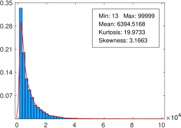
(a) Raw price

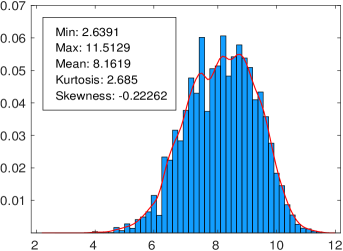
(b) Transformed price

Figure 11: The histogram of historical transaction prices

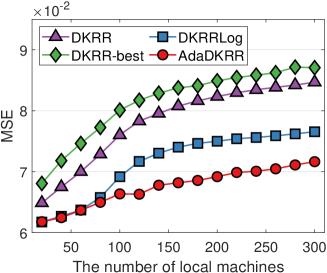
Figure 12: Comparisons of test MSE among the three parameter selection approaches with different numbers of local machines on the data set CarTianchi

The used car data on Tianchi (CarTianchi for short) provided by Alibaba Cloud comes from the used car transaction records of a trading platform, and its goal is to establish models to predict the price of used cars. The data set contains more than $400,000$ samples; each sample is described by 31 attributes, of which $15$ are anonymous and $4$ are masked to protect the confidentiality of the data. The attributes are described in detail in Figure 10, and they are grouped into four categories, including car condition, performance, social factor, and transaction. Note that the $15$ anonymous attributes are classified into the category of transaction for convenience. In the experiment, we selected a subset of $129,710$ samples with price attributes after removing samples with missing values to train and evaluate models. We use the time difference between the sales date (i.e., the create date) and the registration date as an approximation of the usage time and remove the attributes of the sale ID, create date, and registration date. Data binning is applied to the attributes of usage time and power because their values are highly dispersed, and the details are listed in Table 1. The histogram of the target attribute of prices, as well as the skewness and kurtosis, are shown in Figure 11 (a), from which it can be seen that the data distribution does not obey the normal distribution, with a sharp peak and a long tail dragging on the right. Therefore, the target attribute of price is transformed by a logarithmic operation, and the histogram of the transformed price is close to a normal distribution, as shown in Figure 11 (b). The regularization parameter $\lambda$ is chosen from the set $\{\frac{1}{3^{q}}|\frac{1}{3^{q}}\geq 10^{-10},q=0,1,2,\cdots\}$, and the kernel width $\sigma$ is chosen from 10 values that are drawn in a logarithmic, equally spaced interval $[1,10]$.

The relationship between test MSE and the number $m$ of local machines for the compared methods is shown in Figure 12, where $m$ varies from the set $\{20,40,\cdots,300\}$. From the results, we can see that DKRR-best has the worst generalization performance due to the limited number of training samples in local machines; DKRR synthesizes the estimators of local machines and thus achieves better performance than each local estimator; although the logarithmic transformation on the parameters makes DKRRLog superior to DKRR, it can still be significantly improved by AdaDKRR, especially for large numbers of local machines (e.g., $m\geq 100$). The above results demonstrate the effectiveness of the proposed parameter selection approach in distributed learning.

5.2.2 SGEMM GPU Performance Prediction

Over the past decade, GPUs have delivered considerable performance in multi-disciplinary areas such as bioinformatics, astronomy, and machine learning. However, it is still a challenging task to achieve close-to-peak performance on GPUs, as professional programmers must carefully tune their code for various device-specific problems, each of which has its own optimal parameters such as workgroup size, vector data type, tile size, and loop unrolling factor. Therefore, it is important to design effective GPU acceleration models to automatically perform parameter tuning with the data collected from the device.

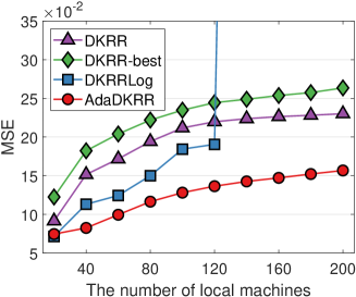
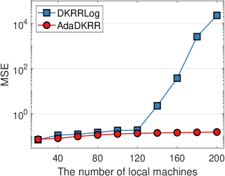
Figure 13: Comparisons of test MSE among the three parameter selection approaches with different numbers of local machines on the data set SGEMM GPU

The data set SGEMM GPU (Nugteren and Codreanu, 2015) considers the running time of dense matrix-matrix multiplication $C=\alpha A^{T}B+\beta C$, as matrix multiplication is a fundamental building block in deep learning and other machine learning methods, where $A\in\mathbb{R}^{K\times M}$, $B\in\mathbb{R}^{K\times N}$, $C\in\mathbb{R}^{M\times N}$, $M=N=K=2048$, $\alpha$ and $\beta$ are constants, and $A^{T}$ is the transpose of $A$. The data set contains $241,600$ samples; each sample includes a possible combination of $14$ parameters of the SGEMM kernel and $4$ running times for this parameter combination. The $14$ parameters and their corresponding domains are as follows:

• Per-matrix 2D tiling at workgroup-level uses the parameters $M_{wg},N_{wg}\in\{16,32,64,$ $128\}$, which correspond to the matrix dimensions of $M$ and $N$, respectively.

• The inner dimension of 2D tiling at workgroup-level uses the parameter $K_{wg}\in\{16,32\}$, which corresponds to the dimension of $K$.

• Local workgroup size uses the parameters $M_{dimC},N_{dimC}\in\{8,16,32\}$.

• Local memory shape uses the parameters $M_{dimA},N_{dimB}\in\{8,16,32\}$.

• The kernel loop unrolling factor is denoted by $K_{wi}\in\{2,8\}$.

• Per-matrix vector widths for loading and storage use parameters $M_{vec},N_{vec}\in\{1,2,4,$ $8\}$, where $M_{vec}$ is for matrices $A$ and $C$, and $N_{vec}$ is for matrix $B$.

• The enabling stride for accessing off-chip memory within a single thread is denoted by $M_{stride},N_{stride}\in\{0,1\}$, where $M_{stride}$ is for matrices $A$ and $C$, and $N_{stride}$ is for matrix $B$.

• Per-matrix manual caching of the 2D workgroup tile can be controlled by parameters $L\$_{A},L\$_{B}\in\{0,1\}$.

In the experiment, the first 14 columns of the data are used as data input, and the average time of the 4 runs is regarded as data output. Similar to the data set CarTianchi, the distribution of the average running time has a sharp peak and a long tail dragging on the right. Therefore, as suggested by Nugteren and Codreanu (2015), we also perform a logarithmic operation on the average running time. The regularization parameter $\lambda$ is chosen from the set $\{\frac{1}{5^{q}}|\frac{1}{5^{q}}\geq 10^{-10},q=0,1,2,\cdots\}$, and the kernel width $\sigma$ is chosen from 10 values that are drawn in a logarithmic, equally spaced interval $[1,100]$.

Figure 13 records the relationship between test MSE and the number of local machines for the compared methods. It can be seen that the performance of these methods on the data set SGEMM GPU is similar to that on the data set CarTianchi. The only difference is that DKRRLog performs extremely poorly in generalization when the number of local machines is larger than $120$. This is because the transformed parameters are far from the optimal parameters in some local machines. These results provide another piece of evidence that the proposed AdaDKRR is stable and effective in selecting parameters.

6 Conclusion

This paper proposed an adaptive parameter selection strategy for distributed learning to settle the data silos. Specifically, by communicating the coefficients of fixed basis functions, we obtained a good approximation of the global estimator and thus determined the algorithm parameters for the global approximation without leaking any sensitive information about the data. From a theoretical perspective, we established optimal rates of excess generalization error for the proposed method in a framework of statistical learning theory by utilizing the idea of low-discrepancy sequences and the classical radial basis function approximation. According to the theoretical findings, as long as the number of local machines is not too large, the proposed method is similar to running KRR on the whole data. The theoretical results demonstrate the efficacy of the proposed method for parameter selection in distributed learning. From an application point of view, we also applied the proposed method to several simulations and two real-world data sets, used car price forecasting and GPU performance prediction. The numerical results verify our theoretical assertions and demonstrate the feasibility and effectiveness of the proposed method in applications.

Appendix A: Training and Testing Flows of AdaDKRR

In this part, we give a detailed implementation of AdaDKRR (with cross-validation) as shown in Algorithm Appendix A: Training and Testing Flows of AdaDKRR, where steps 1–19 are the training process and steps 20–24 are the testing process for a query set. In Algorithm Appendix A: Training and Testing Flows of AdaDKRR, $\mathbb{K}_{\left|D_{j}\right|,n}\in\mathbb{R}^{\left|D_{j}\right|\times n}$ is a kernel matrix with the element in the $i$-th row and the $k$-th column being $K(x_{ij},\xi_{k})$, $\mathbb{K}_{n,n}\in\mathbb{R}^{n\times n}$ is a kernel matrix with the element in the $k$-th row and the $k^{\prime}$-th column being $K(\xi_{k},\xi_{k}^{\prime})$, and $\mathbb{I}_{D}$ is the identity matrix with size $|D|$. $\vec{y}_{D}$ is a vector composed of the outputs of data $D$. In Step 8, $\vec{a}_{j,l,\ell}^{local}:=\left(a_{j,l,1,\ell}^{local},\cdots,a_{j,l,n,\ell}^{local}\right)^{T}=\left(\mathbb{K}_{\left|D_{j,l}^{tr}\right|,n}^{T}\mathbb{K}_{\left|D_{j,l}^{tr}\right|,n}+\mu\left|D_{j,l}^{tr}\right|\mathbb{K}_{n,n}\right)^{\dagger}\mathbb{K}_{\left|D_{j,l}^{tr}\right|,n}^{T}{\vec{f}}_{j,l,\ell}^{tr}$, where $\vec{f}_{j,l,\ell}^{tr}$ is a vector composed of the outputs of data $F_{j,l,\ell}^{tr}$. In Step 11, $\left|D_{l}^{tr}\right|=\sum\limits_{j=1}^{m}\left|D_{j,l}^{tr}\right|$. In Step 13, $\vec{a}_{l,\ell}^{global}:=\left(a_{l,1,\ell}^{global},\cdots,a_{l,n,\ell}^{global}\right)^{T}$. In Step 18, $\vec{\alpha}_{D_{j}}^{\ast}:=\left(\alpha_{1j}^{\ast},\cdots,\alpha_{|D_{j}|j}^{\ast}\right)^{T}=\left(\mathbb{K}_{D_{j},D_{j}}+\lambda_{j}^{\ast}|D_{j}|\mathbb{I}_{D_{j}}\right)^{-1}\vec{y}_{D_{j}}$. Note that we retrain the local estimator $f_{D_{j},\lambda_{j}^{\ast}}$ with all training samples $D_{j}$ under the selected optimal regularization parameter $\lambda_{j}^{\ast}$ in the $j$-th local machine for $j=1,\cdots,m$ to improve the generalization performance of AdaDKRR.

  Algorithm 2  Training and testing flows of AdaDKRR (with cross-validation)

 

1: Input: Training data subset $D_{j}=\{(x_{ij},y_{ij})\}_{i=1}^{|D_{j}|}$ stored in the $j$-th local machine for $j=1,\cdots,m$, query data $D^{\prime}$, and a candidate set of the regularization parameter $\Lambda=\{\lambda_{\ell}\}_{\ell=1}^{L}$.

2: $\#$ Training process

3:for $j=1,\cdots,m$ do

4:     Generate $\iota$ groups of training and validation sets via $\iota$-fold cross validation on data

5:      $D_{j}$, and denote them as $\left\{\left(D_{j,l}^{tr},D_{j,l}^{val}\right)\right\}_{l=1}^{\iota}$. $\triangleright$ Data Split

6:     Generate the same centers $\Xi_{n}=\{\xi_{k}\}_{k=1}^{n}$ satisfying (8) and define a set of functions

7:      $B_{n,K}:=\left\{\sum_{k=1}^{n}a_{k}K_{\xi_{k}}:a_{k}\in\mathbb{R}\right\}$, where $K_{\xi}(x)=K(\xi,x)$. $\triangleright$ Basis Generation

8:end for

9:for $l=1,\cdots,\iota$ do$\triangleright$ Operate on the $l$-th Split

10:     for $j=1,\cdots,m$ do

11:         Given $\lambda_{\ell}\in\Lambda$, run KRR with data $D_{j,l}^{tr}$ to obtain $\triangleright$ Local Processing

$$f_{D_{j,l}^{tr},\lambda_{\ell}}=\arg\min\limits_{f\in\mathcal{H}_{K}}\left\{\frac{1}{\left|D_{j,l}^{tr}\right|}\sum\limits_{(x,y)\in D_{j,l}^{tr}}(f(x)-y)^{2}+\lambda_{\ell}\|f\|_{K}^{2}\right\}.$$

12:         Generate a set of points $F_{j,l,\ell}^{tr}=\left\{\left(x_{i,j},f_{D_{j,l}^{tr},\lambda_{\ell}}(x_{i,j})\right)\right\}_{i=1}^{\left|D_{j,l}^{tr}\right|}$, and run KRR with

13:           $F_{j,l,\ell}^{tr}$ to obtain an approximation of $f_{D_{j,l}^{tr},\lambda_{\ell}}$ by $\triangleright$ Local Approximation

$$\hskip 28.90755ptf_{D_{j,l}^{tr},\lambda_{\ell},n,\mu}^{local}=\arg\min\limits_{f\in B_{n,K}}\frac{1}{\left|D_{j,l}^{tr}\right|}\sum\limits_{(x,y)\in F_{j,l,\ell}^{tr}}(f(x)-y)^{2}+\mu\|f\|_{K}^{2}=\sum\limits_{k=1}^{n}a_{j,l,k,\ell}^{local}K_{\xi_{k}}.$$

14:         Transmit $\left(a_{j,l,k,\ell}^{local}\right)_{k=1,\ell=1}^{n,L}$ to the global machine. $\triangleright$ Communication(I)

15:     end for

16:     Synthesize the coefficients by $a_{l,k,\ell}^{global}=\sum\limits_{j=1}^{m}\frac{\left|D_{j,l}^{tr}\right|}{\left|D_{l}^{tr}\right|}a_{j,l,k,\ell}^{local}$, and communicate the matrix

17:      $\left(a_{l,k,\ell}^{global}\right)_{k=1,\ell=1}^{n,L}$ to each local machine. $\triangleright$ Synthesization and Communication(II)

18:     for $j=1,\cdots,m$ do

19:         Compute $L$ MSEs on the validation set $D_{j,l}^{val}$ by $\triangleright$ Local Validation

$$e_{j,l,\ell}=\frac{1}{|D_{j,l}^{val}|}\left\|\vec{y}_{D_{j,l}^{val}}-\pi_{M}\left(\mathbb{K}_{\left|D_{j,l}^{val}\right|,n}\vec{a}_{l,\ell}^{global}\right)\right\|_{2}^{2}\quad\mbox{for}\quad\ell=1,\cdots,L,$$

20:           and denote the MSE vector with size $L$ as $\vec{e}_{j,l}:=\left(e_{j,l,1},\cdots,e_{j,l,L}\right)^{T}$.

21:     end for

22:end for

23:for $j=1,\cdots,m$ do

24:     Average $\vec{e}_{j,l}$ over the $\iota$-fold, i.e., $\vec{\bar{e}}_{j}=\frac{1}{\iota}\sum\limits_{l=1}^{\iota}\vec{e}_{j,l}$, and select the optimal parameter

25:      $\lambda_{j}^{\ast}\in\Lambda$ with the minimum element in the vector $\vec{\bar{e}}_{j}$. $\triangleright$ Parameter Selection

26:     Run KRR with data $D_{j}$ under the optimal parameter $\lambda_{j}^{\ast}$ to obtain$\triangleright$ Retraining

$$f_{D_{j},\lambda_{j}^{\ast}}=\arg\min\limits_{f\in\mathcal{H}_{K}}\left\{\frac{1}{|D_{j}|}\sum\limits_{(x,y)\in D_{j}}(f(x)-y)^{2}+\lambda_{j}^{\ast}\|f\|_{K}^{2}\right\}=\sum\limits_{i=1}^{|D_{j}|}\alpha_{ij}^{\ast}K_{x_{ij}}.$$

27:end for

28: $\#$ Testing process

29:Distribute the query data $D^{\prime}$ to $m$ local machines.

30:for $j=1,\cdots,m$ do

31:     Compute a vector of size $|D^{\prime}|$ by $\pi_{M}f_{D_{j},\lambda_{j}^{\ast}}(D^{\prime})=\pi_{M}\left(\mathbb{K}_{\left|D^{\prime}\right|,\left|D_{j}\right|}\vec{\alpha}_{D_{j}}^{\ast}\right)$, and commu-

32:      nicate it to the global machine. $\triangleright$ Communication(III)

33:end for

34:Synthesize the final estimate by

$$\overline{f}^{Ada}_{D,\vec{\lambda}^{\ast}}(D^{\prime}):=\sum_{j=1}^{m}\frac{|D_{j}|}{|D|}\pi_{M}f_{D_{j},\lambda_{j}^{\ast}}(D^{\prime}).$$

$\triangleright$ Global Estimates

35: Output: The global estimate $\overline{f}^{Ada}_{D,\vec{\lambda}^{\ast}}(D^{\prime})$ for the query data $D^{\prime}$.

 

Appendix B: Proofs

In this part, we use the well-developed integral operator approach (Smale and Zhou, 2007; Lin et al., 2017; Rudi et al., 2015) to prove our main results. Our main novelty in the proof is the detailed analysis of the role of the weight $\frac{|D_{j}|}{|D|}$ in (1) and a tight bound on local approximation. Our proofs are divided into four steps: error decomposition, local approximation and global approximation, generalization error of DKRR, and generalization error of AdaDKRR.

6.1 Error decomposition based on integral operators

Let $D$ be a set of data drawn i.i.d. according to a distribution $\rho$. Denote by $S_{D}:\mathcal{H}_{K}\rightarrow\mathbb{R}^{|D|}$ the sampling operator on $\mathcal{H}_{K}$

$$S_{D}f:=\{f(x_{i})\}_{(x_{i},y_{i})\in D}.$$

Its scaled adjoint $S_{D}^{T}:\mathbb{R}^{|D|}\rightarrow\mathcal{H}_{K}$ is

$$S_{D}^{T}{\bf c}:=\frac{1}{|D|}\sum_{(x_{i},y_{i})\in D}c_{i}K_{x_{i}},\qquad{\bf c}\in\mathbb{R}^{|D|}.$$

Let $L_{K,D}$ be the empirical version of $L_{K}$ and it is defined by

$$L_{K,D}f:=S_{D}^{T}S_{D}f=\frac{1}{|D|}\sum_{(x,y)\in D}f(x)K_{x}.$$

Then we have (Smale and Zhou, 2005)

$$f_{D,\lambda}=(L_{K,D}+\lambda I)^{-1}S^{T}_{D}y_{D},$$ (25)

where $y_{D}:=(y_{1},\dots,y_{|D|})^{T}$.

To present the error decomposition of DKRR, we need the following lemma that can be easily deduced from (Guo et al., 2017a, Prop.4) or (Chang et al., 2017b, Prop.5).

Lemma 4

Let $\overline{f}_{D,\vec{\lambda}}$ be defined by (1). We have

$$E\left[\|\overline{f}_{D,\vec{\lambda}}-f_{\rho}\|_{\rho}^{2}\right]\leq 2\sum_{j=1}^{m}\frac{|D_{j}|^{2}}{|D|^{2}}E\left[\left\|f_{D_{j},\lambda_{j}}-f^{\diamond}_{D_{j},\lambda_{j}}\right\|_{\rho}^{2}\right]+2\sum_{j=1}^{m}\frac{|D_{j}|}{|D|}E\left[\left\|f^{\diamond}_{D_{j},\lambda_{j}}-f_{\rho}\right\|_{\rho}^{2}\right],$$ (26)

where

$$f^{\diamond}_{D,\lambda}:=(L_{K,D}+\lambda I)^{-1}L_{K,D}f_{\rho}$$ (27)

is the noise-free version of $f_{D,\lambda}$.

With the help of the above lemma, we can derive the following error decomposition for DKRR based on integral operators.

Proposition 5

Let $\overline{f}_{D,\vec{\lambda}}$ be defined by (1). If Assumption 2 holds with $\frac{1}{2}\leq r\leq 1$, then

$$E\left[\|\overline{f}_{D,\vec{\lambda}}-f_{\rho}\|_{\rho}^{2}\right] \leq 2\sum_{j=1}^{m}\frac{|D_{j}|}{|D|}\lambda^{2r}_{j}E\left[\mathcal{Q}_{D_{j},\lambda}^{4r}\right]\|h_{\rho}\|_{\rho}^{2}+2\sum_{j=1}^{m}\frac{|D_{j}|^{2}}{|D|^{2}}E\left[\mathcal{Q}_{D_{j},\lambda_{j}}^{4}\mathcal{P}^{2}_{D_{j},\lambda_{j}}\right],$$ (28)

where

$$\mathcal{Q}_{D,\lambda} := \left\|(L_{K,D}+\lambda I)^{-1/2}(L_{K}+\lambda I)^{1/2}\right\|,$$ (29)

$$\mathcal{P}_{D,\lambda} := \left\|(L_{K}+\lambda I)^{-1/2}(L_{K,D}f_{\rho}-S^{T}_{D}y_{D})\right\|_{K}.$$ (30)

Proof Proof. Due to (25) and (27), we obtain

$$f^{\diamond}_{D,\lambda}-f_{\rho}=((L_{K,D}+\lambda I)^{-1}L_{K,D}-I)f_{\rho}=\lambda(L_{K,D}+\lambda I)^{-1}f_{\rho}$$ (31)

and

$$f^{\diamond}_{D,\lambda}-f_{D,\lambda}=(L_{K,D}+\lambda I)^{-1}(L_{K,D}f_{\rho}-S_{D}^{T}y_{D}).$$ (32)

Then, we get from (29), (30), (32), (31) with $D=D_{j}$, $\lambda=\lambda_{j}$, and Assumption 2 with $\frac{1}{2}\leq r\leq 1$ that for any $1\leq j\leq m$, there holds

$$\|f^{\diamond}_{D_{j},\lambda_{j}}-f_{\rho}\|_{\rho}\leq\lambda_{j}\|(L_{K}+\lambda_{j}I)^{1/2}(L_{K,D_{j}}+\lambda_{j}I)^{-1}f_{\rho}\|_{K}$$

$$\leq \lambda_{j}\mathcal{Q}_{D_{j},\lambda_{j}}\|(L_{K,D_{j}}+\lambda_{j}I)^{-1/2}L_{K}^{r-1/2}\|\|h_{\rho}\|_{\rho}\leq\lambda^{r}_{j}\mathcal{Q}_{D_{j},\lambda}^{2r}\|h_{\rho}\|_{\rho}$$

and

$$\|f_{D_{j},\lambda_{j}}-f^{\diamond}_{D_{j},\lambda_{j}}\|_{\rho}\leq\|(L_{K}+\lambda_{j}I)^{1/2}(L_{K,D_{j}}+\lambda_{j}I)^{-1}(S^{T}_{D_{j}}y_{D_{j}}-L_{K,D}f_{\rho})\|_{K}\leq\mathcal{Q}_{D_{j},\lambda_{j}}^{2}\mathcal{P}_{D_{j},\lambda_{j}}.$$

Plugging the above two estimates into (26), we then obtain

$$\frac{1}{2}E\left[\|\overline{f}_{D,\vec{\lambda}}-f_{\rho}\|_{\rho}^{2}\right]\leq\sum_{j=1}^{m}\frac{|D_{j}|}{|D|}\lambda^{2r}_{j}E\left[\mathcal{Q}_{D_{j},\lambda}^{4r}\right]\|h_{\rho}\|_{\rho}^{2}+\sum_{j=1}^{m}\frac{|D_{j}|^{2}}{|D|^{2}}E\left[\mathcal{Q}_{D_{j},\lambda_{j}}^{4}\mathcal{P}^{2}_{D_{j},\lambda_{j}}\right].$$

This completes the proof of Proposition 5.  

We next derive an error decomposition for AdaDKRR in the following proposition.

Proposition 6

For any $\delta>0$ and any $\lambda\in\Lambda$, if Assumption 1 holds and $|D_{j}^{tr}|\sim|D_{j}^{val}|$, then

$$E\left[\left\|\overline{f}^{Ada}_{D,\vec{\lambda^{*}}}-f_{\rho}\right\|_{\rho}^{2}\right]\leq\frac{C^{\prime}_{1}(1+\log|\Lambda|)m}{|D|}$$ (33)

$$+ 4\min_{\lambda\in\Lambda}\left\{\sum_{j=1}^{m}\frac{|D_{j}^{tr}|}{|D^{tr}|}E\left[\left\|{f}^{global}_{D^{tr},{\lambda},n,\mu}-\sum_{j=1}^{m}\frac{|D_{j}^{tr}|}{|D^{tr|}}f_{D_{j},{\lambda}}\right\|_{\rho}^{2}\right]+E\left[\left\|\sum_{j=1}^{m}\frac{|D_{j}^{tr}|}{|D^{tr|}}f_{D_{j},{\lambda}}-f_{\rho}\right\|_{\rho}^{2}\right]\right\},$$

where $C_{1}^{\prime}$ is an absolute constant.

To prove the above proposition, we need the following lemma which can be found in (Györfi et al., 2002, Theorem 7.1) (see also (Caponnetto and Yao, 2010) for a probabilistic argument).

Lemma 7

For a given data set $D$, let $D^{tr}$ and $D^{val}$ be the training set and validation set respectively. Under Assumption 1, for any $\delta>0$ and any $\lambda\in\Lambda$, there holds

$$E\left[\left\|\pi_{M}f_{D^{tr},{\color[rgb]{1,0,0}\hat{\lambda}}}-f_{\rho}\right\|_{\rho}^{2}\right]\leq(1+\delta)\min_{\lambda\in\Lambda}E\left[\left\|\pi_{M}f_{D^{tr},\lambda}-f_{\rho}\right\|_{\rho}^{2}\right]+C^{\prime}\frac{1+\log|\Lambda|}{|D^{val}|},$$

where $C^{\prime}=M^{2}(16/\delta+35+19\delta)$.

With the help of the above lemma, we can prove Proposition 6 as follows.

Proof Proof of Proposition 6. Due to (7), we have from Lemma 7, $|D_{j}^{val}|\sim|D_{j}^{tr}|$, (6), and Jensen’s inequality that

$$E\left[\left\|\overline{f}^{Ada}_{D,\vec{\lambda^{*}}}-f_{\rho}\right\|_{\rho}^{2}\right]\leq\sum_{j=1}^{m}\frac{|D_{j}^{tr}|}{|D^{tr}|}E\left[\left\|\pi_{M}{f}^{global}_{D^{tr},\lambda^{*}_{j},n,\mu}-f_{\rho}\right\|_{\rho}^{2}\right]$$

$$\leq \sum_{j=1}^{m}\frac{|D_{j}^{tr}|}{|D^{tr}|}\left((1+\delta)\min_{\lambda\in\Lambda}E\left[\left\|\pi_{M}{f}^{global}_{D^{tr},\lambda,n,\mu}-f_{\rho}\right\|_{\rho}^{2}\right]+\frac{C^{\prime}(1+\log|\Lambda|)}{|D_{j}^{val}|}\right)$$

$$\leq (1+\delta)\sum_{j=1}^{m}\frac{|D_{j}^{tr}|}{|D^{tr}|}\min_{\lambda\in\Lambda}E\left[\left\|{f}^{global}_{D^{tr},\lambda,n,\mu}-f_{\rho}\right\|_{\rho}^{2}\right]+\frac{C^{\prime}_{1}(1+\log|\Lambda|)m}{{|D|}}$$

$$\leq \frac{C^{\prime}_{1}m(1+\log|\Lambda|)}{|D|}+2(1+\delta)\min_{\lambda\in\Lambda}\left\{\sum_{j=1}^{m}\frac{|D_{j}^{tr}|}{|D^{tr}|}E\left[\left\|{f}^{global}_{D^{tr},{\lambda},n,\mu}-\sum_{j=1}^{m}\frac{|D_{j}^{tr}|}{|D^{tr|}}f_{D_{j},{\lambda}}\right\|_{\rho}^{2}\right]\right.$$

$$\left.+E\left[\left\|\sum_{j=1}^{m}\frac{|D_{j}^{tr}|}{|D^{tr|}}f_{D_{j},{\lambda}}-f_{\rho}\right\|_{\rho}^{2}\right]\right\},$$

where we use $(a+b)^{2}\leq 2a^{2}+2b^{2}$ in the last inequality and $C^{\prime}$, $C_{1}$ are absolute constants. This completes the proof of Proposition 6 by setting $\delta=1$.  

6.2 Local approximation and global approximation

Due to Proposition 6, it is crucial to derive the error of the global approximation (5) as well as the local approximation (4). In this appendix only, we denote by ${f}^{loc}_{D,\lambda,\mu}$ the local approximation (4) with $D_{j}^{tr}=D$, $s=|D|$, and $\lambda_{\ell}=\lambda$ for the sake of brevity. The derived error of local approximation is shown in the following proposition.

Proposition 8

If (11) holds with $1/2\leq r\leq 1$, then we have

$$\left\|{f}^{loc}_{D,\lambda,\mu}-f_{D,\lambda}\right\|_{\rho}\leq\mu^{r}\left\|h_{\rho}\right\|_{\rho}\left(\left(\mathcal{Q}_{D,\mu}\mathcal{Q}_{D,\mu}^{*}+1\right)\mathcal{Q}_{\Xi_{n},\mu}^{2r}+\mathcal{Q}_{D,\mu}^{2r}\right)$$ (34)

$$+ \mu^{1/2}\left(\lambda^{-1/2}\mathcal{Q}^{2}_{D,\lambda}\mathcal{P}_{D,\lambda}+\lambda^{r-1/2}\mathcal{Q}_{D,\lambda}^{2r-1}\|h\|_{\rho}\right)\left(\mathcal{Q}_{D,\mu}+\left(\mathcal{Q}_{D,\mu}\mathcal{Q}_{D,\mu}^{*}+1\right)\mathcal{Q}_{\Xi_{n},\mu}\right),$$

where $\|\cdot\|$ denotes the operator norm and

$$\mathcal{Q}_{D,\mu}^{*}:=\left\|(L_{K}+\mu I)^{-1/2}(L_{K,D}+\mu I)^{1/2}\right\|.$$ (35)

Before providing the proof of the above proposition, we introduce several interesting tools. Let $P_{\Xi_{n}}$ be the projection from $\mathcal{H}_{K}$ to $B_{n,K}$. Then for an arbitrary $\nu>0$, there holds

$$(I-P_{\Xi_{n}})^{\nu}=I-P_{\Xi_{n}}.$$ (36)

Let $T_{\Xi_{n}}:B_{n,K}\rightarrow\mathbb{R}^{n}$ be a sampling operator defined by $T_{\Xi_{n}}f:=\{f(x_{i})\}_{x_{i}\in\Xi_{n}}$ such that the range of its adjoint operator $T^{T}_{\Xi_{n}}$ is exactly in $B_{n,K}$, and let $U\Sigma V^{T}$ be the SVD of $T_{\Xi_{n}}$. Then we have

$$V^{T}V=I,\qquad VV^{T}=P_{\Xi_{n}}.$$ (37)

Write

$$g_{\Xi_{n},\mu}(L_{K,D}):=V(V^{T}L_{K,D}V+\mu I)^{-1}V^{T}.$$ (38)

Then it can be found in (9) and (Rudi et al., 2015) that

$${f}^{loc}_{D,\lambda,\mu}=g_{\Xi_{n},\mu}(L_{K,D})L_{K,D}f_{D,\lambda}.$$ (39)

For an arbitrary bounded linear operator $B$, it follows from (37) and (38) that

$$g_{\Xi_{n},\mu}(L_{K,D})(L_{K,D}+\mu I)VBV^{T}=VBV^{T}.$$ (40)

Inserting $B=(V^{T}L_{K,D}V+\mu I)^{-1}$ into (40), it is easy to derive (Sun et al., 2021)

$$\|(L_{K,D}+\mu I)^{1/2}g_{\Xi_{n},\mu}(L_{K,D})(L_{K,D}+\mu I)^{1/2}\|\leq 1.$$ (41)

Besides the above tools, we also need the following two lemmas that can be found in (Rudi et al., 2015, Proposition 3) and (Rudi et al., 2015, Proposition 6), respectively.

Lemma 9

Let $\mathcal{H}$, $\mathcal{K}$, and $\mathcal{F}$ be three separable Hilbert spaces. Let $Z:\mathcal{H}\rightarrow\mathcal{K}$ be a bounded linear operator and $P$ be a projection operator on $\mathcal{H}$ such that $\mbox{range}P=\overline{\mbox{range}Z^{T}}$. Then for any bounded linear operator $F:\mathcal{F}\rightarrow\mathcal{H}$ and any $\lambda>0$, we have

$$\|(I-P)F\|\leq\lambda^{1/2}\left\|(Z^{T}Z+\lambda I)^{-1/2}F\right\|.$$

Lemma 10

Let $\mathcal{H}$ and $\mathcal{K}$ be two separable Hilbert spaces, $A:\mathcal{H}\rightarrow\mathcal{H}$ be a positive linear operator, $V_{\mathcal{H},\mathcal{K}}:\mathcal{H}\rightarrow\mathcal{K}$ be a partial isometry, and $B:\mathcal{K}\rightarrow\mathcal{K}$ be a bounded operator. Then for all $0\leq r^{*},s^{*}\leq 1/2$, there holds

$$\left\|A^{r^{*}}V_{\mathcal{H},\mathcal{K}}BV_{\mathcal{H},\mathcal{K}}^{T}A^{s^{*}}\right\|\leq\left\|(V_{\mathcal{H},\mathcal{K}}^{T}AV_{H,K})^{r^{*}}B(V_{\mathcal{H},\mathcal{K}}^{T}AV_{\mathcal{H},\mathcal{K}})^{s^{*}}\right\|.$$

With the help of the above lemmas and the important properties of $g_{D_{m},\mu}$ in (40) and (41), we prove Proposition 8 as follows.

Proof Proof of Proposition 8. The triangle inequality yields

$$\|f^{loc}_{D,\lambda,\mu}-f_{D,\lambda}\|_{\rho}\leq\mathcal{A}_{n}(D,\lambda,\mu)+\mathcal{C}_{n}(D,\lambda,\mu),$$ (42)

where

$$\mathcal{A}_{n}(D,\lambda,\mu) = \left\|(g_{\Xi_{n},\mu}(L_{K,D})L_{K,D}-I)P_{\Xi_{n}}f_{D,\lambda}\right\|_{\rho},$$

$$\mathcal{C}_{n}(D,\lambda,\mu) = \left\|(g_{\Xi_{n},\mu}(L_{K,D})L_{K,D}-I)(I-P_{\Xi_{n}})f_{D,\lambda}\right\|_{\rho}.$$

We first bound $\mathcal{A}_{n}(D,\lambda,\mu)$. It follows from (40) with $B=I$ that

$$P_{\Xi_{n}}=g_{\Xi_{n},\mu}(L_{K,D})(L_{K,D}+\mu I)P_{\Xi_{n}},$$

which together with the definition of $\mathcal{A}_{n}(D,\lambda,\mu)$ yields

$$\mathcal{A}_{n}(D,\lambda,\mu)=\mu\|g_{\Xi_{n},\mu}(L_{K,D})P_{\Xi_{n}}f_{D,\lambda}\|_{\rho}.$$

Then we have from the triangle inequality that

$$\mathcal{A}_{n}(D,\lambda,\mu) \leq \mu\left\|g_{\Xi_{n},\mu}(L_{K,D})P_{\Xi_{n}}f_{\rho}\right\|_{\rho}+\mu\left\|g_{\Xi_{n},\mu}(L_{K,D})P_{\Xi_{n}}(f_{D,\lambda}-f_{\rho})\right\|_{\rho}$$ (43)

$$=: \mathcal{A}_{n,1}(D,\mu)+\mathcal{A}_{n,2}(D,\lambda,\mu).$$

To bound $\mathcal{A}_{n,1}(D,\mu)$, noting that $L_{K,D}$ is a positive operator, we have $\|(V^{T}(L_{K,D}+\mu I)V)^{r-1}\|\leq\mu^{r-1}$ for $r\leq 1$ (Rudi et al., 2015). Recalling further (37) and the Cordes inequality (Bhatia, 2013)

$$\|A^{u}B^{u}\|\leq\|AB\|^{u},\qquad 0<u\leq 1$$ (44)

for arbitrary positive operators $A$ and $B$, we get from Lemma 10 with $A=(L_{K,D}+\mu I)$, $V_{\mathcal{H},\mathcal{K}}=V$, $B=(V^{T}L_{K,D}V+\mu I)^{-1}$, $r^{*}=1/2$, and $s^{*}=r-1/2$ that

$$\mathcal{A}_{n,1}(D,\mu)\leq\mu\left\|L_{K}^{1/2}g_{{\Xi_{n}},\mu}(L_{K,D})VV^{T}L_{K}^{r-1/2}\right\|\left\|h_{\rho}\right\|_{\rho}$$ (45)

$$\leq \mu\mathcal{Q}_{D,\mu}^{2r}\left\|h_{\rho}\right\|_{\rho}\left\|(L_{K,D}+\mu I)^{1/2}g_{{\Xi_{n}},\mu}(L_{K,D})VV^{T}(L_{K,D}+\mu I)^{r-1/2}\right\|$$

$$\leq \mu\mathcal{Q}_{D,\mu}^{2r}\left\|(V^{T}(L_{K,D}+\mu I)V)^{1/2}(V^{T}(L_{K,D}+\mu I)V)^{-1}(V^{T}(L_{K,D}+\mu I)V)^{r-1/2}\right\|\left\|h_{\rho}\right\|_{\rho}$$

$$\leq \mu\mathcal{Q}_{D,\mu}^{2r}\left\|(V^{T}(L_{K,D}+\mu I))^{r-1}V\right\|\left\|h_{\rho}\right\|_{\rho}$$

$$\leq \mu^{r}\mathcal{Q}_{D,\mu}^{2r}\left\|h_{\rho}\right\|_{\rho}.$$

To bound $\mathcal{A}_{n,2}(D,\lambda,\mu)$, we need the following standard estimate of $\|f_{D,\lambda}-f_{\rho}\|_{K}$ (Caponnetto and De Vito, 2007; Steinwart et al., 2009; Lin et al., 2017; Chang et al., 2017b), which can be derived in a way similar to that used to prove Proposition 5. Under (11) with $r\leq 1$, there holds

$$\|f_{D,\lambda}-f_{\rho}\|_{K}\leq\lambda^{-1/2}\mathcal{Q}^{2}_{D,\lambda}\mathcal{P}_{D,\lambda}+\lambda^{r-1/2}\mathcal{Q}_{D,\lambda}^{2r-1}\|h\|_{\rho}.$$ (46)

Then, it follows from (37), (44), and Lemma 10 with $A=(L_{K,D}+\mu I)$, $V_{H,K}=V$, $B=(V^{T}L_{K,D}V+\mu I)^{-1}$, $r^{*}=1/2$, and $s^{*}=0$ that

$$\mathcal{A}_{n,2}(D,\lambda,\mu)\leq\mu\left\|L_{K}^{1/2}g_{{\Xi_{n}},\mu}(L_{K,D})VV^{T}\right\|\left\|f_{D,\lambda}-f_{\rho}\right\|_{K}$$ (47)

$$\leq \mu\mathcal{Q}_{D,\mu}\left(\lambda^{-1/2}\mathcal{Q}^{2}_{D,\lambda}\mathcal{P}_{D,\lambda}+\lambda^{r-1/2}\mathcal{Q}_{D,\lambda}^{2r-1}\|h\|_{\rho}\right)\left\|(L_{K,D}+\mu I)^{1/2}g_{\Xi_{n},\mu}(L_{K,D})VV^{T}\right\|$$

$$\leq \mu\mathcal{Q}_{D,\mu}\left(\lambda^{-1/2}\mathcal{Q}^{2}_{D,\lambda}\mathcal{P}_{D,\lambda}+\lambda^{r-1/2}\mathcal{Q}_{D,\lambda}^{2r-1}\|h\|_{\rho}\right)\left\|(V^{T}(L_{K,D}+\mu I)V)^{-1/2}\right\|$$

$$\leq \mu^{1/2}\mathcal{Q}_{D,\mu}\left(\lambda^{-1/2}\mathcal{Q}^{2}_{D,\lambda}\mathcal{P}_{D,\lambda}+\lambda^{r-1/2}\mathcal{Q}_{D,\lambda}^{2r-1}\|h\|_{\rho}\right).$$

Plugging (45) and (47) into (43), we obtain

$$\mathcal{A}_{n}(D,\lambda,\mu)\leq\mu^{r}\mathcal{Q}_{D,\mu}^{2r}\|h_{\rho}\|_{\rho}+\mu^{1/2}\mathcal{Q}_{D,\mu}\left(\lambda^{-1/2}\mathcal{Q}^{2}_{D,\lambda}\mathcal{P}_{D,\lambda}+\lambda^{r-1/2}\mathcal{Q}_{D,\lambda}^{2r-1}\|h\|_{\rho}\right).$$ (48)

We next bound $\mathcal{C}_{n}(D,\lambda,\mu)$. Similar to the above, we have

$$\mathcal{C}_{n}(D,\lambda,\mu) \leq \left\|(g_{\Xi_{n},\mu}(L_{K,D})L_{K,D}-I)(I-P_{\Xi_{n}})f_{\rho}\right\|_{\rho}$$ (49)

$$+ \left\|(g_{\Xi_{n},\mu}(L_{K,D})L_{K,D}-I)(I-P_{\Xi_{n}})(f_{D,\lambda}-f_{\rho})\right\|_{\rho}$$

$$=: \mathcal{C}_{n,1}(D,\mu)+\mathcal{C}_{n,2}(D,\lambda,\mu).$$

Due to Lemma 9, we have

$$\left\|(I-P_{\Xi_{n}})(L_{K}+\mu I)^{1/2}\right\|\leq\mu^{1/2}\left\|(L_{K,\Xi_{n}}+\mu I)^{-1/2}(L_{K}+\mu I)^{1/2}\right\|\leq\mu^{1/2}\mathcal{Q}_{\Xi_{n},\mu}.$$ (50)

Then, it follows from (41), (44), and (36) with $\tau=2r$ that

$$\mathcal{C}_{n,1}(D,\mu)\leq\left\|L_{K}^{1/2}g_{\Xi_{n},\mu}(L_{K,D})L_{K,D}(I-P_{\Xi_{n}})L_{K}^{r-1/2}\right\|\left\|h_{\rho}\right\|_{\rho}$$ (51)

$$+ \left\|L_{K}^{1/2}(I-P_{\Xi_{n}})L_{K}^{r-1/2}\right\|\left\|h_{\rho}\right\|_{\rho}$$

$$\leq \mathcal{Q}_{D,\mu}\mathcal{Q}_{D,\mu}^{*}\left\|(L_{K,D}+\mu I)^{1/2}g_{\Xi_{n},\mu}(L_{K,D})(L_{K,D}+\mu I)^{1/2}\right\|$$

$$\times \left\|(L_{K}+\mu I)^{1/2}(I-P_{\Xi_{n}})^{2r}L_{K}^{r-1/2}\right\|\left\|h_{\rho}\right\|_{\rho}$$

$$+ \left\|(L_{K}+\mu I)^{1/2}(I-P_{\Xi_{n}})^{2r}L_{K}^{r-1/2}\right\|\left\|h_{\rho}\right\|_{\rho}$$

$$\leq \left(\mathcal{Q}_{D,\mu}\mathcal{Q}_{D,\mu}^{*}+1\right)\left\|h_{\rho}\right\|_{\rho}\left\|(L_{K}+\mu I)^{1/2}(I-P_{\Xi_{n}})\right\|\left\|(I-P_{\Xi_{n}})^{2r-1}L_{K}^{r-1/2}\right\|$$

$$\leq \left(\mathcal{Q}_{D,\mu}\mathcal{Q}_{D,\mu}^{*}+1\right)\left\|h_{\rho}\right\|_{\rho}\mu^{r}\mathcal{Q}_{\Xi_{n},\mu}^{2r}.$$

Noting (46), we get from (36), (41), (44), and (50) again that

$$\mathcal{C}_{n,2}(D,\lambda,\mu)$$

$$\leq \left\|L_{K}^{1/2}g_{\Xi_{n},\mu}(L_{K,D})L_{K,D}(I-P_{\Xi_{n}})\right\|\left(\lambda^{-1/2}\mathcal{Q}^{2}_{D,\lambda}\mathcal{P}_{D,\lambda}+\lambda^{r-1/2}\mathcal{Q}_{D,\lambda}^{2r-1}\|h\|_{\rho}\right)$$

$$+ \left\|L_{K}^{1/2}(I-P_{\Xi_{n}})\right\|\left(\lambda^{-1/2}\mathcal{Q}^{2}_{D,\lambda}\mathcal{P}_{D,\lambda}+\lambda^{r-1/2}\mathcal{Q}_{D,\lambda}^{2r-1}\|h\|_{\rho}\right)$$

$$\leq \mathcal{Q}_{D,\mu}\mathcal{Q}_{D,\mu}^{*}\left\|(L_{K,D}+\mu I)^{1/2}g_{\Xi_{n},\mu}(L_{K,D})(L_{K,D}+\mu I)^{1/2}\right\|$$

$$\times \left\|(L_{K}+\mu I)^{1/2}(I-P_{\Xi_{n}})\right\|\left(\lambda^{-1/2}\mathcal{Q}^{2}_{D,\lambda}\mathcal{P}_{D,\lambda}+\lambda^{r-1/2}\mathcal{Q}_{D,\lambda}^{2r-1}\|h\|_{\rho}\right)$$

$$+ \left\|(L_{K}+\mu I)^{1/2}(I-P_{\Xi_{n}})\right\|\left(\lambda^{-1/2}\mathcal{Q}^{2}_{D,\lambda}\mathcal{P}_{D,\lambda}+\lambda^{r-1/2}\mathcal{Q}_{D,\lambda}^{2r-1}\|h\|_{\rho}\right)$$

$$\leq \left(\mathcal{Q}_{D,\mu}\mathcal{Q}_{D,\mu}^{*}+1\right)\left(\lambda^{-1/2}\mathcal{Q}^{2}_{D,\lambda}\mathcal{P}_{D,\lambda}+\lambda^{r-1/2}\mathcal{Q}_{D,\lambda}^{2r-1}\|h\|_{\rho}\right)\left\|(L_{K}+\mu I)^{1/2}(I-P_{\Xi_{n}})\right\|$$

$$\leq \left(\mathcal{Q}_{D,\mu}\mathcal{Q}_{D,\mu}^{*}+1\right)\left(\lambda^{-1/2}\mathcal{Q}^{2}_{D,\lambda}\mathcal{P}_{D,\lambda}+\lambda^{r-1/2}\mathcal{Q}_{D,\lambda}^{2r-1}\|h\|_{\rho}\right)\mu^{1/2}\mathcal{Q}_{\Xi_{n},\mu}.$$ (53)

Inserting (51) and (6.2) into (49), we have

$$\mathcal{C}_{n}(D,\lambda,\mu) \leq \left(\mathcal{Q}_{D,\mu}\mathcal{Q}_{D,\mu}^{*}+1\right)\left(\lambda^{-1/2}\mathcal{Q}^{2}_{D,\lambda}\mathcal{P}_{D,\lambda}+\lambda^{r-1/2}\mathcal{Q}_{D,\lambda}^{2r-1}\|h\|_{\rho}\right)\mu^{1/2}\mathcal{Q}_{\Xi_{n},\mu}$$ (54)

$$+ \left(\mathcal{Q}_{D,\mu}\mathcal{Q}_{D,\mu}^{*}+1\right)\|h_{\rho}\|_{\rho}\mu^{r}\mathcal{Q}_{\Xi_{n},\mu}^{2r}.$$

Plugging (48) and (54) into (42), we get

$$\left\|{f}^{loc}_{D,\lambda,\mu}-f_{D,\lambda}\right\|_{\rho}\leq\mu^{r}\left\|h_{\rho}\right\|_{\rho}\left(\left(\mathcal{Q}_{D,\mu}\mathcal{Q}_{D,\mu}^{*}+1\right)\mathcal{Q}_{\Xi_{n},\mu}^{2r}+\mathcal{Q}_{D,\mu}^{2r}\right)$$

$$+ \mu^{1/2}\left(\lambda^{-1/2}\mathcal{Q}^{2}_{D,\lambda}\mathcal{P}_{D,\lambda}+\lambda^{r-1/2}\mathcal{Q}_{D,\lambda}^{2r-1}\|h\|_{\rho}\right)\left(\mathcal{Q}_{D,\mu}+\left(\mathcal{Q}_{D,\mu}\mathcal{Q}_{D,\mu}^{*}+1\right)\mathcal{Q}_{\Xi_{n},\mu}\right).$$

This completes the proof of Proposition 8.  

Based on Proposition 8, we can derive an error estimate for the global approximation directly.

Proposition 11

If (11) holds with $1/2\leq r\leq 1$, then

$$\left\|{f}^{global}_{D^{tr},\lambda,\mu}-\sum_{j=1}^{m}\frac{|D_{j}^{tr}|}{|D^{tr}|}f_{D_{j},\lambda}\right\|_{\rho}\leq\sum_{j=1}^{m}\frac{|D_{j}^{tr}|}{|D^{tr}|}\left[\mu^{r}\left\|h_{\rho}\right\|_{\rho}\left(\left(\mathcal{Q}_{D_{j}^{tr},\mu}\mathcal{Q}_{D_{j}^{tr},\mu}^{*}+1\right)\mathcal{Q}_{\Xi_{n},\mu}^{2r}+\mathcal{Q}_{D_{j}^{tr},\mu}^{2r}\right)\right.$$

$$+\left.\mu^{1/2}\left(\lambda^{-1/2}\mathcal{Q}^{2}_{D_{j}^{tr},\lambda}\mathcal{P}_{D_{j}^{tr},\lambda}+\lambda^{r-1/2}\mathcal{Q}_{D_{j}^{tr},\lambda}^{2r-1}\left\|h\right\|_{\rho}\right)\left(\mathcal{Q}_{D_{j}^{tr},\mu}+\left(\mathcal{Q}_{D_{j}^{tr},\mu}\mathcal{Q}_{D_{j}^{tr},\mu}^{*}+1\right)\mathcal{Q}_{\Xi_{n},\mu}\right)\right].$$

Proof Proof. It follows from (5) and Jensen’s inequality that

$$\left\|{f}^{global}_{D^{tr},\lambda,\mu}-\sum_{j=1}^{m}\frac{|D_{j}^{tr}|}{|D^{tr}|}f_{D_{j},\lambda}\right\|_{\rho}=\left\|\sum_{j=1}^{m}\frac{|D_{j}^{tr}|}{|D^{tr}|}\left({f}^{loc}_{D_{j}^{tr},\lambda,\mu}-f_{D_{j},\lambda}\right)\right\|_{\rho}\leq\sum_{j=1}^{m}\frac{|D_{j}^{tr}|}{|D^{tr}|}\left\|{f}^{loc}_{D_{j}^{tr},\lambda,\mu}-f_{D_{j},\lambda}\right\|_{\rho}.$$

But Proposition 8 with $D=D_{j}^{tr}$ for $j=1,\dots,m$ yields

$$\left\|{f}^{loc}_{D_{j}^{tr},\lambda,\mu}-f_{D_{j}^{tr},\lambda}\right\|_{\rho}\leq\mu^{r}\left\|h_{\rho}\right\|_{\rho}\left(\left(\mathcal{Q}_{D_{j}^{tr},\mu}\mathcal{Q}_{D_{j}^{tr},\mu}^{*}+1\right)\mathcal{Q}_{\Xi_{n},\mu}^{2r}+\mathcal{Q}_{D_{j}^{tr},\mu}^{2r}\right)$$

$$+ \mu^{1/2}\left(\lambda^{-1/2}\mathcal{Q}^{2}_{D_{j}^{tr},\lambda}\mathcal{P}_{D_{j}^{tr},\lambda}+\lambda^{r-1/2}\mathcal{Q}_{D_{j}^{tr},\lambda}^{2r-1}\|h\|_{\rho}\right)\left(\mathcal{Q}_{D_{j}^{tr},\mu}+\left(\mathcal{Q}_{D_{j}^{tr},\mu}\mathcal{Q}_{D_{j}^{tr},\mu}^{*}+1\right)\mathcal{Q}_{\Xi_{n},\mu}\right).$$

Combining the above two estimates proves Proposition 11.  

6.3 Proof of Theorem 1 and Corollary 2

To prove Theorem 1, it suffices to bound $E\left[\mathcal{Q}_{D_{j},\lambda}^{4r}\right]$ and $E\left[\mathcal{Q}_{D_{j},\lambda_{j}}^{4}\mathcal{P}^{2}_{D_{j},\lambda_{j}}\right]$, which requires several auxiliary lemmas. The first one focuses on bounding $\mathcal{P}_{D,\lambda}$ derived in (Caponnetto and De Vito, 2007; Lin et al., 2017).

Lemma 12

Let $D$ be a set of samples drawn i.i.d. according to $\rho$ and $0<\delta<1$. Under Assumption 1, with confidence at least $1-\delta$, there holds

$$\mathcal{P}_{D,\lambda} \leq 2M(\kappa+1)\left(\frac{1}{|D|\sqrt{\lambda}}+\sqrt{\frac{\mathcal{N}(\lambda)}{|D|}}\right)\log\frac{2}{\delta}.$$ (55)

The second one aims to bounding

$$\mathcal{R}_{D,\lambda}:=\left\|(L_{K}+\lambda I)^{-1/2}(L_{K}-L_{K,D})(L_{K}+\lambda I)^{-1/2}\right\|$$ (56)

that can be deduced from (Lin et al., 2021, Lemma 6).

Lemma 13

Let $D$ be a set of samples drawn i.i.d. according to $\rho$. If $\frac{1}{|D|}<\lambda\leq 1$ and $\mathcal{N}(\lambda)\geq 1$, then

$$P\left[\mathcal{R}_{D,\lambda}\geq\frac{1}{4}\right]\leq 4\exp\left\{-\frac{\sqrt{\lambda|D|}}{C_{1}^{*}(1+\log\mathcal{N}(\lambda))}\right\},$$ (57)

where $C_{1}^{*}:=4\max\{(\kappa^{2}+1)/3,2\sqrt{\kappa^{2}+1}\}$.

Due to the definition of $\mathcal{R}_{D,\lambda}$, the bounds of $\mathcal{Q}_{D,\lambda}$ and $\mathcal{Q}^{*}_{D,\lambda}$ can be given in the following lemma, whose proof is rather standard.

Lemma 14

If $\mathcal{R}_{D,\lambda}\leq 1/4$, there holds

$$\mathcal{Q}_{D,\lambda}\leq\frac{2\sqrt{3}}{3}$$ (58)

and

$$\mathcal{Q}^{*}_{D,\lambda}\leq\frac{\sqrt{6}}{2}.$$ (59)

Proof Proof. A direct computation yields

$$(L_{K}+\lambda I)^{1/2}(L_{K,D}+\lambda I)^{-1}(L_{K}+\lambda I)^{1/2}$$

$$= (L_{K}+\lambda I)^{1/2}[(L_{K,D}+\lambda I)^{-1}-(L_{K}+\lambda I)^{-1}](L_{K}+\lambda I)^{1/2}+I=I$$

$$+ (L_{K}+\lambda I)^{-1/2}(L_{K}-L_{K,D})(L_{K}+\lambda I)^{-1/2}(L_{K}+\lambda I)^{1/2}(L_{K,D}+\lambda I)^{-1}(L_{K}+\lambda I)^{1/2}.$$

Thus,

$$\left\|(L_{K}+\lambda I)^{1/2}(L_{K,D}+\lambda I)^{-1}(L_{K}+\lambda I)^{1/2}\right\|$$

$$\leq 1+\frac{1}{4}\left\|(L_{K}+\lambda I)^{1/2}(L_{K,D}+\lambda I)^{-1}(L_{K}+\lambda I)^{1/2}\right\|.$$

This implies

$$\|(L_{K}+\lambda I)^{1/2}(L_{K,D}+\lambda I)^{-1}(L_{K}+\lambda I)^{1/2}\|\leq\frac{4}{3}$$

and (58). Then,

$$\left\|(L_{K,D}+\lambda I)^{-1/2}(L_{K}-L_{K,D})(L_{K,D}+\lambda I)^{-1/2}\right\|\leq\mathcal{Q}_{D,\lambda}^{2}\mathcal{R}_{D,\lambda}\leq\frac{1}{3}.$$

But

$$\left\|(L_{K,D}+\lambda I)^{1/2}(L_{K}+\lambda I)^{-1}(L_{K,D}+\lambda I)^{1/2}\right\|$$

$$\leq 1+\frac{1}{3}\left\|(L_{K,D}+\lambda I)^{1/2}(L_{K}+\lambda I)^{-1}(L_{K,D}+\lambda I)^{1/2}\right\|.$$

Therefore, we have

$$\left\|(L_{K,D}+\lambda I)^{1/2}(L_{K}+\lambda I)^{-1}(L_{K,D}+\lambda I)^{1/2}\right\|\leq\frac{3}{2}.$$

This completes the proof of Lemma 14.  

For further use, we also need the following probability to expectation formula (Lin et al., 2023).

Lemma 15

Let $0<\delta<1$, and let $\xi\in\mathbb{R}_{+}$ be a random variable. If $\xi\leq\mathcal{A}\log^{b}\frac{c}{\delta}$ holds with confidence $1-\delta$ for some $\mathcal{A},b,c>0$, then

$$E[\xi]\leq c\Gamma(b+1)\mathcal{A},$$

where $\Gamma(\cdot)$ is the Gamma function.

With the help of the above lemmas, we can derive the bounds of $E\left[\mathcal{Q}_{D,\lambda}^{4}\mathcal{P}_{D,\lambda}^{2}\right]$ and $E\left[\mathcal{Q}_{D,\lambda}^{4r}\right]$ as follows.

Lemma 16

Under Assumption 1, if $\lambda|D|\geq(2vC_{1}^{*}(\log(1+\kappa)+2))^{2}\log^{4}|D|$ for some $v\geq 1$, then

$$E\left[\mathcal{Q}_{D,\lambda}^{2v}\mathcal{P}_{D,\lambda}^{v}\right] \leq C_{0}^{*}\left(\left(\frac{1}{|D|\sqrt{\lambda}}+\sqrt{\frac{\mathcal{N}(\lambda)}{|D|}}\right)^{v}+|D|^{-v/2}\right),$$ (60)

$$E\left[\mathcal{Q}_{D,\lambda}^{u}\right] \leq 5(2+\kappa)^{u/2},\qquad\forall\ 0\leq u\leq 4v,$$ (61)

$$E[(\mathcal{Q}_{D,\lambda}^{*})^{u}] \leq 5(4+\kappa)^{u/2},\qquad\forall\ 0\leq u\leq 4v,$$ (62)

where $C_{0}^{*}:=2(2(\kappa+1)M)^{v}\max\{\gamma(v+1)2^{v},2\kappa^{v}\}$.

Proof Proof. If $R_{D,\lambda}\leq 1/4$, it follows from Lemma 14 and Lemma 12 that, with confidence $1-\delta$, there holds

$$\mathcal{Q}_{D,\lambda}^{2v}\mathcal{P}^{v}_{D,\lambda}\leq\left(4M(\kappa+1)\left(\frac{1}{|D|\sqrt{\lambda}}+\sqrt{\frac{\mathcal{N}(\lambda)}{|D|}}\right)\log\frac{2}{\delta}\right)^{v}.$$

Then Lemma 15 with $\mathcal{A}=\left(4M(\kappa+1)\left(\frac{1}{|D|\sqrt{\lambda}}+\sqrt{\frac{\mathcal{N}(\lambda)}{|D|}}\right)\right)^{v}$, $b=v$, and $c=2$ implies

$$E\left[\mathcal{Q}_{D,\lambda}^{2v}\mathcal{P}_{D,\lambda}^{v}|R_{D,\lambda}\leq 1/4\right]\leq 2\Gamma(v+1)\left(4M(\kappa+1)\left(\frac{1}{|D|\sqrt{\lambda}}+\sqrt{\frac{\mathcal{N}(\lambda)}{|D|}}\right)\right)^{v}.$$ (63)

But $\lambda|D|\geq(2vC_{1}^{*}(\log(1+\kappa)+2))^{2}\log^{4}|D|$ together with Lemma 13, $\mathcal{N}(\lambda)\leq\kappa\lambda^{-1}$, and $\lambda\geq|D|^{-1}$ yields

$$P\left[R_{D,\lambda}>1/2\right]\leq 4\exp\left\{-\frac{2vC_{1}^{*}(\log(1+\kappa)+2)\log^{2}{|D|}}{C_{1}^{*}(2+\log((\kappa+1)|D|))}\right\}$$ (64)

$$\leq 4\exp\left\{-2v\log|D|\right\}=4|D|^{-2v}.$$

Therefore, we get from $\mathcal{Q}_{D,\lambda}^{2v}\mathcal{P}^{v}_{D,\lambda}\leq(2(\kappa+1)\kappa M\lambda^{-3/2})^{v}$ and (64) that

$$E\left[\mathcal{Q}_{D,\lambda}^{2v}\mathcal{P}^{v}_{D,\lambda}\right]=E\left[\mathcal{Q}_{D,\lambda_{j}}^{4}\mathcal{P}^{2}_{D,\lambda_{j}}|R_{D,\lambda}\leq 1/4\right]P[R_{D,\lambda}\leq 1/4]$$

$$+ E\left[\mathcal{Q}_{D,\lambda_{j}}^{4}\mathcal{P}^{2}_{D,\lambda_{j}}|R_{D,\lambda}>1/4\right]P[R_{D,\lambda}>1/4]$$

$$\leq 2\Gamma(v+1)\left(4M(\kappa+1)\left(\frac{1}{|D|\sqrt{\lambda}}+\sqrt{\frac{\mathcal{N}(\lambda)}{|D|}}\right)\right)^{v}+4(2(\kappa+1)\kappa M\lambda^{-3/2})^{v}|D|^{-2v}$$

$$\leq 2(2(\kappa+1)M)^{v}\max\{\Gamma(v+1)2^{v},2\kappa^{v}\}\left(\left(\frac{1}{|D|\sqrt{\lambda}}+\sqrt{\frac{\mathcal{N}(\lambda)}{|D|}}\right)^{v}+|D|^{-v/2}\right).$$

This proves (60). Noting further

$$\mathcal{Q}_{D,\lambda}\leq\sqrt{1+\kappa}\lambda^{-1/2},$$

we have from $0\leq u\leq 4v$, Lemma 14, and (64) that

$$E\left[\mathcal{Q}_{D,\lambda}^{u}\right] \leq E\left[\mathcal{Q}_{D,\lambda}^{u}|R_{D,\lambda}>1/4\right]P[R_{D,\lambda}>1/4]+E\left[\mathcal{Q}_{D,\lambda}^{u}|R_{D,\lambda}\leq 1/4\right]P[R_{D,\lambda}\leq 1/4]$$

$$\leq 4(1+\kappa)^{u/2}|D|^{u/2-2v}+2^{u/2}\leq 5(2+\kappa)^{u/2}.$$

The bound of (62) can be derived in the same way. This completes the proof of Lemma 16.  

We then turn to prove Theorem 1.

Proof Proof of Theorem 1. Noting (15) with $C_{1}:=(4C_{1}^{*}(\log(1+\kappa)+2))^{2}$, we have $\lambda|D_{j}|\geq(4C_{1}^{*}(\log(1+\kappa)+2))^{2}\log^{4}|D_{j}|$ for all $j=1,\dots,m$. Then, it follows from Lemma 16 with $v=2$, $u=4r$, (15), $r\geq 1/2$, and (16) that

$$\sum_{j=1}^{m}\frac{|D_{j}|}{|D|}\lambda_{j}^{2r}\|h_{\rho}\|_{\rho}^{2}E\left[\mathcal{Q}_{D_{j},\lambda_{j}}^{2r}\right]$$ (65)

$$\leq C_{2}^{*}\left(\sum_{j:|D_{j}|\geq|D|^{\frac{1}{2r+s}}\log^{4}|D|}\frac{|D_{j}|}{|D|}|D|^{-\frac{2r}{2r+s}}+\sum_{j:|D_{j}|\leq|D|^{\frac{1}{2r+s}}\log^{4}|D|}\frac{|D_{j}|}{|D|}|D_{j}|^{-2r}\log^{8r}|D|\right)$$

$$\leq 2C_{2}^{*}|D|^{-\frac{2r}{2r+s}},$$

where $C_{2}^{*}:=5(2+\kappa)^{2r}(4C_{1}^{*}(\log(1+\kappa)+2))^{4r}\|h_{\rho}\|_{\rho}^{2}$. Furthermore, it follows from Lemma 16 with $v=2$, Assumption 3, and (15) that

$$\sum_{j=1}^{m}\frac{|D_{j}|^{2}}{|D|^{2}}E\left[\mathcal{Q}_{D_{j},\lambda_{j}}^{4}\mathcal{P}^{2}_{D_{j},\lambda_{j}}\right]$$

$$\leq 80M^{2}(\kappa+1)^{4}\sum_{j=1}^{m}\frac{|D_{j}|^{2}}{|D|^{2}}\left(\left(\frac{1}{|D_{j}|\sqrt{\lambda_{j}}}+\sqrt{\frac{\mathcal{N}(\lambda_{j})}{|D_{j}|}}\right)^{2}+|D_{j}|^{-1}\right)$$

$$\leq 160M^{2}(\kappa+1)^{4}|D|^{-1}\sum_{j=1}^{m}\left(2|D|^{-1}\lambda_{j}^{-1}+\frac{|D_{j}|}{|D|}\mathcal{N}(\lambda_{j})\right)$$

$$\leq 160(C_{0}+2)M^{2}(\kappa+1)^{4}|D|^{-1}\sum_{j=1}^{m}\left(|D|^{-1}\lambda_{j}^{-1}+\frac{|D_{j}|}{|D|}\lambda_{j}^{-s}\right).$$

But (15) and (16) yield

$$\sum_{j=1}^{m}\left(\lambda_{j}^{-1}+\frac{|D_{j}|}{|D|}\lambda_{j}^{-s}\right)$$

$$\leq \sum_{j:|D_{j}|\geq|D|^{\frac{1}{2r+s}}\log^{4}|D|}\left(|D|^{-1}\lambda_{j}^{-1}+\frac{|D_{j}|}{|D|}\lambda_{j}^{-s}\right)$$

$$+ \sum_{j:|D_{j}|<|D|^{\frac{1}{2r+s}}\log^{4}|D|}\left(|D|^{-1}\lambda_{j}^{-1}+\frac{|D_{j}|}{|D|}\lambda_{j}^{-s}\right)$$

$$\leq (4C_{1}^{*}(\log(1+\kappa)+2))^{-2s}\left(m|D|^{\frac{-2r-s+1}{2r+s}}+|D|^{\frac{s}{2r+s}}+\log^{-4}|D|+|D|^{\frac{s}{2r+s}}\right)$$

$$\leq 4(4C_{1}^{*}(\log(1+\kappa)+2))^{-2s}|D|^{\frac{s}{2r+s}}.$$

Thus, we have

$$\sum_{j=1}^{m}\frac{|D_{j}|^{2}}{|D|^{2}}E\left[\mathcal{Q}_{D_{j},\lambda_{j}}^{4}\mathcal{P}^{2}_{D_{j},\lambda_{j}}\right]\leq C_{3}^{*}|D|^{-\frac{2r}{2r+s}},$$ (66)

where $C_{3}^{*}:=640(C_{0}+2)M^{2}(\kappa+1)^{4}(4C_{1}^{*}(\log(1+\kappa)+2))^{-2s}.$ Plugging (65) and (66) into Proposition 5, we complete the proof of Theorem 1 with $C_{2}=4C_{2}^{*}+2C_{3}^{*}$.  

The proof of Corollary 2 is almost the same as above. We present it for the sake of completeness.

Proof Proof of Corollary 2. Setting $C_{1}:=(4C_{1}^{*}(\log(1+\kappa)+2))^{2}$, we have $\lambda|D_{j}|\geq(4C_{1}^{*}(\log(1+\kappa)+2))^{2}\log^{4}|D_{j}|$ for all $j=1,\dots,m$. Then, it follows from Lemma 16 with $u=4r$ and $v=2$ that

$$\sum_{j=1}^{m}\frac{|D_{j}|}{|D|}\lambda_{j}^{2r}\|h_{\rho}\|_{\rho}^{2}E\left[\mathcal{Q}_{D_{j},\lambda}^{2r}\right]\leq C_{2}^{*}\sum_{j=1}^{m}\frac{|D_{j}|}{|D|}|D|^{-\frac{2r}{2r+s}}=C_{2}^{*}|D|^{-\frac{2r}{2r+s}}.$$

Furthermore, it follows from Lemma 16 with $v=2$, Assumption 3, and (18) that

$$\sum_{j=1}^{m}\frac{|D_{j}|^{2}}{|D|^{2}}E\left[\mathcal{Q}_{D_{j},\lambda_{j}}^{4}\mathcal{P}^{2}_{D_{j},\lambda_{j}}\right]$$

$$\leq 160(C_{0}+2)M^{2}(\kappa+1)^{4}|D|^{-1}\sum_{j=1}^{m}\left(|D|^{-1}\lambda_{j}^{-1}+\frac{|D_{j}|}{|D|}\lambda_{j}^{-s}\right)$$

$$\leq 160(C_{0}+2)M^{2}(\kappa+1)^{4}(4C_{1}^{*}(\log(1+\kappa)+2))^{-2s}|D|^{-1}\left(m|D|^{\frac{-2r-s+1}{2r+s}}+|D|^{\frac{s}{2r+s}}\right)$$

$$\leq C_{3}^{*}|D|^{-\frac{2r}{2r+s}}.$$

Plugging the above two estimates into Proposition 5 completes the proof of Corollary 2.  

6.4 Proof of Theorem 3

In this part, we use Theorem 1 and Proposition 6 to prove Theorem 3. Firstly, we present a detailed bound of the global approximation as follows.

Proposition 17

Under Assumption 1 and Assumption 2 with $1/2\leq r\leq 1$, if $\rho_{X}$ is a uniform distribution, $\mu\geq(8C_{1}^{*}(\log(1+\kappa)+2))^{2}\max_{j=1,\dots,m}\frac{\log^{4}|D_{j}^{tr}|}{|D_{j}^{tr}|}$, $\Xi_{n}$ satisfies (8) for some $c,\beta>0$, and $n$ satisfies $\mu n^{\beta}\geq 2c$, then for any $\lambda\in(\mu,1)$, there holds

$$E\left[\left\|{f}^{global}_{D^{tr},\lambda,\mu}-\sum_{j=1}^{m}\frac{|D_{j}^{tr}|}{|D^{tr}|}f_{D_{j},\lambda}\right\|_{\rho}^{2}\right]$$

$$\leq C_{4}\mu^{2r}+C_{4}\mu\left(\lambda^{2r-1}+\sum_{j=1}^{m}\frac{|D_{j}^{tr}|}{|D^{tr}|}\left(\left(\frac{1}{|D_{j}^{tr}|{\lambda}}+\sqrt{\frac{\mathcal{N}(\lambda)}{\lambda|D_{j}^{tr}|}}\right)^{2}+|D_{j}^{tr}|^{-1}\right)\right),$$

where $C_{4}$ is a constant depending only on $\|h_{\rho}\|_{\rho},M,r,c$, and $\beta$.

To prove the above proposition, we need the following preliminary lemma.

Lemma 18

If $\rho_{X}$ is a uniform distribution, $\Xi_{n}$ satisfies (8) for some $c,\beta>0$, and $n$ satisfies $\mu n^{\beta}\geq 2c$, then

$$\mathcal{Q}_{\Xi_{n},\mu}\leq\sqrt{2}.$$ (67)

Proof Proof. From the definition of the operator norm $\|\cdot\|$ and the fact $\|f\|_{K}=\sup\limits_{\|g\|_{K}\leq 1}\langle f,g\rangle_{K}$, we obtain

$$\|L_{K}-L_{K,\Xi_{n}}\|=\sup_{\|f\|_{K}\leq 1}\|((L_{K,\Xi_{n}}-L_{K})f\|_{K}=\sup_{\|f\|_{K}\leq 1}\sup_{\|g\|_{K}\leq 1}\langle(L_{K,\Xi_{n}}-L_{K})f,g\rangle_{K}$$

$$= \sup_{\|g\|_{K}\leq 1,\|f\|_{K}\leq 1}\left|\left\langle\int_{\mathcal{X}}f(x^{\prime})K_{x^{\prime}}d\rho_{X}-\frac{1}{n}\sum_{k=1}^{n}f(\xi_{k})K_{\xi_{k}},g\right\rangle_{K}\right|$$

$$= \sup_{\|g\|_{K}\leq 1,\|f\|_{K}\leq 1}\left|\int_{\mathcal{X}}f(x^{\prime})\langle K_{x^{\prime}},g\rangle_{K}d\rho_{X}-\frac{1}{n}\sum_{k=1}^{n}f(\xi_{k})\langle K_{\xi_{k}},g\rangle_{K}\right|$$

$$= \sup_{\|g\|_{K}\leq 1,\|f\|_{K}\leq 1}\left|\int_{\mathcal{X}}f(x^{\prime})g(x^{\prime})d\rho_{X}-\frac{1}{n}\sum_{k=1}^{n}f(\xi_{k})g(x_{i})\right|.$$

Then, it follows from (8) that

$$\|L_{K,\Xi_{n}}-L_{K}\|\leq cn^{-\beta}.$$

Therefore,

$$\|(L_{K}+\mu I)^{-1/2}(L_{K}-L_{K,\Xi_{n}})(L_{K}+\mu I)^{-1/2}\|\leq c\mu^{-1}n^{-\beta}.$$

Then it follows from $\mu n^{\beta}\geq 2c$ that

$$\|(L_{K}+\mu I)^{-1/2}(L_{K}-L_{K,\Xi_{n}})(L_{K}+\mu I)^{-1/2}\|\leq 1/2.$$

Noting further

$$\mathcal{Q}_{D,\Xi_{n}}^{2}=\left\|(L_{K}+\mu I)^{1/2}(L_{K,\Xi_{n}}+\mu I)^{-1}(L_{K}+\mu I)^{1/2}\right\|$$

$$\leq \left\|(L_{K}+\mu I)^{1/2}\left[(L_{K,\Xi_{n}}+\mu I)^{-1}-(L_{K}+\mu I)^{-1}\right](L_{K}+\mu I)^{1/2}\right\|+1$$

$$\leq \frac{1}{2}\mathcal{Q}_{D,\Xi_{n}}^{2}+1,$$

we then obtain $\mathcal{Q}_{D,\Xi_{n}}\leq\sqrt{2}$. This completes the proof of Lemma 18.  

With the help of the above two lemmas and Proposition 11, we are in a position to prove Proposition 17 as follows.

Proof Proof of Proposition 17. Due to Proposition 11, Hölder’s inequality, Jensen’s inequality, and the basic inequalities $(a+b)^{2}\leq 2a^{2}+2b^{2}$ and $(a+b)^{4}\leq 8a^{4}+8b^{4}$ for $a,b\geq 0$, we have

$$E\left[\left\|{f}^{global}_{D^{tr},\lambda,\mu}-\sum_{j=1}^{m}\frac{|D_{j}^{tr}|}{|D^{tr}|}f_{D_{j},\lambda}\right\|_{\rho}^{2}\right]$$

$$\leq 4\mu^{2r}\|h_{\rho}\|_{\rho}^{2}\sum_{j=1}^{m}\frac{|D_{j}^{tr}|}{|D^{tr}|}E\left[\left(\mathcal{Q}_{D_{j}^{tr},\mu}\mathcal{Q}_{D_{j}^{tr},\mu}^{*}+1\right)^{2}\mathcal{Q}_{\Xi_{n},\mu}^{4r}\right]+4\mu^{2r}\|h_{\rho}\|_{\rho}^{2}\sum_{j=1}^{m}\frac{|D_{j}^{tr}|}{|D^{tr}|}E\left[\mathcal{Q}_{D_{j}^{tr},\mu}^{4r}\right]$$

$$+ 16\mu\sum_{j=1}^{m}\frac{|D_{j}^{tr}|}{|D^{tr}|}\left(E\left[\lambda^{-2}\mathcal{Q}^{8}_{D_{j}^{tr},\lambda}\mathcal{P}^{4}_{D_{j}^{tr},\lambda}+\lambda^{4r-2}\mathcal{Q}_{D_{j}^{tr},\lambda}^{8r-4}\|h\|_{\rho}^{4}\right]\right)^{1/2}$$

$$\times \left(E\left[\mathcal{Q}_{D_{j}^{tr},\mu}^{4}+\left(\mathcal{Q}_{D_{j}^{tr},\mu}\mathcal{Q}_{D_{j}^{tr},\mu}^{*}+1\right)^{4}\mathcal{Q}^{4}_{\Xi_{n},\mu}\right]\right)^{1/2}.$$

Using (61), (62), and Lemma 18 with $u=4$ and $v=4$, we get from Hölder’s inequality and $\mu\geq(8C_{1}^{*}(\log(1+\kappa)+2))^{2}\max_{j=1,\dots,m}\frac{\log^{4}|D_{j}^{tr}|}{|D_{j}^{tr}|}$ that

$$E\left[\left(\mathcal{Q}_{D_{j}^{tr},\mu}\mathcal{Q}_{D_{j}^{tr},\mu}^{*}+1\right)^{2}\mathcal{Q}_{\Xi_{n},\mu}^{4r}\right]\leq 2^{2r+1}(1+5(2+\kappa)(4+\kappa)).$$

Moreover, it follows from (61) with $u=4r$ and $v=4$ that

$$E\left[\mathcal{Q}_{D_{j}^{tr},\mu}^{4r}\right]\leq 5(2+\kappa)^{2r}.$$

Using (60) with $v=4$ and (61) with $u=8r-4$ and $v=4$, we obtain from $\lambda\geq(8C_{1}^{*}(\log(1+\kappa)+2))^{2}\max_{j=1,\dots,m}\frac{\log^{4}|D_{j}^{tr}|}{|D_{j}^{tr}|}$ that

$$\left(E\left[\lambda^{-2}\mathcal{Q}^{8}_{D_{j}^{tr},\lambda}\mathcal{P}^{4}_{D_{j}^{tr},\lambda}+\lambda^{4r-2}\mathcal{Q}_{D_{j}^{tr},\lambda}^{8r-4}\|h\|_{\rho}^{4}\right]\right)^{1/2}$$

$$\leq \lambda^{-1}(C_{0}^{*})^{1/2}\left(\left(\frac{1}{|D_{j}^{tr}|\sqrt{\lambda}}+\sqrt{\frac{\mathcal{N}(\lambda)}{|D_{j}^{tr}|}}\right)^{2}+|D_{j}^{tr}|^{-1}\right)+\lambda^{2r-1}\|h\|_{\rho}^{2}\sqrt{5}(2+\kappa)^{2r-1}.$$

Furthermore, Lemma 16 with $u=4$ and Lemma 18 yield

$$\left(E\left[\mathcal{Q}_{D_{j}^{tr},\mu}^{4}+\left(\mathcal{Q}_{D_{j}^{tr},\mu}\mathcal{Q}_{D_{j}^{tr},\mu}^{*}+1\right)^{4}\mathcal{Q}^{4}_{\Xi_{n},\mu}\right]\right)^{1/2}$$

$$\leq \left(E\left[\mathcal{Q}_{D_{j}^{tr},\mu}^{4}\right]\right)^{1/2}+4\sqrt{2}\left(1+\left(E\left[\mathcal{Q}_{D_{j}^{tr},\mu}^{8}\right]\right)^{1/2}\left(E\left[\left(\mathcal{Q}^{*}_{D_{j}^{tr},\mu}\right)^{8}\right]\right)^{1/2}\right)^{1/2}$$

$$\leq \sqrt{5}(2+\kappa)+4\sqrt{2}+4\sqrt{2}4\sqrt{10}(2+\kappa)(4+\kappa).$$

Combining all the above estimates, we have from $\mu\geq(8C_{1}^{*}(\log(1+\kappa)+2))^{2}\max_{j=1,\dots,m}\frac{\log^{4}|D_{j}^{tr}|}{|D_{j}^{tr}|}$ that

$$E\left[\left\|{f}^{global}_{D^{tr},\lambda,\mu}-\sum_{j=1}^{m}\frac{|D_{j}^{tr}|}{|D^{tr}|}f_{D_{j},\lambda}\right\|_{\rho}^{2}\right]\leq\mu^{2r}\|h_{\rho}\|_{\rho}^{2}\left(2^{2r+3}(1+5(2+\kappa)(4+\kappa))+20(2+\kappa)^{2r}\right)$$

$$+ 16\mu\left(\sqrt{5}(2+\kappa)+4\sqrt{2}+4\sqrt{2}4\sqrt{10}(2+\kappa)(4+\kappa)\right)$$

$$\times \left(\lambda^{-1}\left(C_{0}^{*}\right)^{1/2}\sum_{j=1}^{m}\frac{|D_{j}^{tr}|}{|D^{tr}|}\left(\left(\frac{1}{|D_{j}^{tr}|\sqrt{\lambda}}+\sqrt{\frac{\mathcal{N}(\lambda)}{|D_{j}^{tr}|}}\right)^{2}+|D_{j}^{tr}|^{-1}\right)+\lambda^{2r-1}\|h\|_{\rho}^{2}\sqrt{5}(2+\kappa)^{2r-1}\right)$$

$$\leq C_{4}\mu^{2r}+C_{4}\mu\left(\lambda^{2r-1}+\sum_{j=1}^{m}\frac{|D_{j}^{tr}|}{|D^{tr}|}\left(\left(\frac{1}{|D_{j}^{tr}|{\lambda}}+\sqrt{\frac{\mathcal{N}(\lambda)}{\lambda|D_{j}^{tr}|}}\right)^{2}+|D_{j}^{tr}|^{-1}\right)\right),$$

where $C_{4}$ is a constant depending only on $\kappa$, $M$, $r$, $C_{0}^{*}$, and $\|h_{\rho}\|_{\rho}$. This completes the proof of Proposition 17.  

Finally, we prove Theorem 3.

Proof Proof of Theorem 3. Let $\bar{\lambda}:=C_{1}|D|^{-\frac{1}{2r+s}}$. We have from $|D_{j}|\geq|D|^{\frac{1}{2r+s}}\log^{4}|D|$ and Assumption 3 that

$$\sum_{j=1}^{m}\frac{|D_{j}^{tr}|}{|D^{tr}|}\left(\left(\frac{1}{|D_{j}^{tr}|{\bar{\lambda}}}+\sqrt{\frac{\mathcal{N}(\bar{\lambda})}{\bar{\lambda}|D_{j}^{tr}|}}\right)^{2}+|D_{j}^{tr}|^{-1}\right)\leq\tilde{C}_{2}m|D|^{-\frac{2r-1}{2r+s}},$$

where $\tilde{C}_{2}$ is a constant depending only on $C_{0}$ and $C_{1}$. Then it follows from Proposition 17 that, under (20), there holds

$$E\left[\left\|{f}^{global}_{D^{tr},\bar{\lambda},\mu}-\sum_{j=1}^{m}\frac{|D_{j}^{tr}|}{|D^{tr}|}f_{D_{j},\lambda}\right\|_{\rho}^{2}\right]\leq\tilde{C}_{3}\left(\mu^{2r}+\mu|D|^{-\frac{2r-1}{2r+s}}\right),$$

where $\tilde{C}_{3}$ is a constant depending only on $C_{4},C_{1}$, and $C_{0}$. Furthermore, it follows from Corollary 2 that, under (20), there holds

$$E\left[\left\|\sum_{j=1}^{m}\frac{|D_{j}^{tr}|}{|D^{tr|}}f_{D_{j},\bar{\lambda}}-f_{\rho}\right\|_{\rho}^{2}\right]\leq C_{2}|D|^{-\frac{2r}{2r+s}}.$$

Plugging the above two estimates into Proposition 6 and noting $\mu\leq|D|^{-\frac{1}{2r+s}}$, we have

$$E\left[\left\|\overline{f}^{Ada}_{D,\vec{\lambda^{*}}}-f_{\rho}\right\|_{\rho}^{2}\right]\leq C_{5}\left(m\frac{\log|\Lambda|}{|D|}+|D|^{-\frac{2r}{2r+s}}\right),$$

where $C_{5}$ is a constant depending only on $\tilde{C}_{2}$, $C_{2}$, and $C_{1}^{\prime}$. This completes the proof of Theorem 3.

References

- Balcan et al. (2012) Maria Florina Balcan, Avrim Blum, Shai Fine, and Yishay Mansour. Distributed learning, communication complexity and privacy. In Conference on Learning Theory, pages 26–1. JMLR Workshop and Conference Proceedings, 2012.
- Bhatia (2013) Rajendra Bhatia. Matrix Analysis, volume 169. Springer Science & Business Media, 2013.
- Blanchard and Krämer (2016) Gilles Blanchard and Nicole Krämer. Convergence rates of kernel conjugate gradient for random design regression. Analysis and Applications, 14(06):763–794, 2016.
- Blanchard et al. (2019) Gilles Blanchard, Peter Mathé, and Nicole Mücke. Lepskii principle in supervised learning. arXiv preprint arXiv:1905.10764, 2019.
- Caponnetto and De Vito (2007) Andrea Caponnetto and Ernesto De Vito. Optimal rates for the regularized least-squares algorithm. Foundations of Computational Mathematics, 7(3):331–368, 2007.
- Caponnetto and Yao (2010) Andrea Caponnetto and Yuan Yao. Cross-validation based adaptation for regularization operators in learning theory. Analysis and Applications, 8(02):161–183, 2010.
- Celisse and Wahl (2021) Alain Celisse and Martin Wahl. Analyzing the discrepancy principle for kernelized spectral filter learning algorithms. J. Mach. Learn. Res., 22:76–1, 2021.
- Chang et al. (2017a) Xiangyu Chang, Shao-Bo Lin, and Yao Wang. Divide and conquer local average regression. Electronic Journal of Statistics, 11:1326–1350, 2017a.
- Chang et al. (2017b) Xiangyu Chang, Shao-Bo Lin, and Ding-Xuan Zhou. Distributed semi-supervised learning with kernel ridge regression. The Journal of Machine Learning Research, 18(1):1493–1514, 2017b.
- Cucker and Zhou (2007) Felipe Cucker and Ding Xuan Zhou. Learning Theory: an Approximation Theory Viewpoint, volume 24. Cambridge University Press, 2007.
- Davenport et al. (2012) Thomas H. Davenport, Paul Barth, and Randy Bean. How ‘Big Data’ Is Different. MIT Sloan Management Review, 2012.
- De Vito et al. (2010) Ernesto De Vito, Sergei Pereverzyev, and Lorenzo Rosasco. Adaptive kernel methods using the balancing principle. Foundations of Computational Mathematics, 10(4):455–479, 2010.
- Dekel et al. (2012) Ofer Dekel, Ran Gilad-Bachrach, Ohad Shamir, and Lin Xiao. Optimal distributed online prediction using mini-batches. Journal of Machine Learning Research, 13(6):165–202, 2012.
- Dick (2011) Josef Dick. Higher order scrambled digital nets achieve the optimal rate of the root mean square error for smooth integrands. The Annals of Statistics, 39(3):1372–1398, 2011.
- Dick and Pillichshammer (2010) Josef Dick and Friedrich Pillichshammer. Digital nets and sequences: discrepancy theory and quasi–Monte Carlo integration. Cambridge University Press, 2010.
- Dicker et al. (2017) Lee H Dicker, Dean P Foster, and Daniel Hsu. Kernel ridge vs. principal component regression: Minimax bounds and the qualification of regularization operators. Electronic Journal of Statistics, 11(1):1022–1047, 2017.
- Fan et al. (2014) Jianqing Fan, Fang Han, and Han Liu. Challenges of big data analysis. National Science Review, 1(2):293–314, 2014.
- Feng et al. (2021) Han Feng, Shao-Bo Lin, and Ding-Xuan Zhou. Radial basis function approximation with distributively stored data on spheres. arXiv:2112.02499, 2021.
- Fischer and Steinwart (2020) Simon Fischer and Ingo Steinwart. Sobolev norm learning rates for regularized least-squares algorithms. J. Mach. Learn. Res., 21(205):1–38, 2020.
- Guo et al. (2017a) Zheng-Chu Guo, Shao-Bo Lin, and Ding-Xuan Zhou. Learning theory of distributed spectral algorithms. Inverse Problems, 33(7):074009, 2017a.
- Guo et al. (2017b) Zheng-Chu Guo, Lei Shi, and Qiang Wu. Learning theory of distributed regression with bias corrected regularization kernel network. Journal of Machine Learning Research, 18(1):4237–4261, 2017b.
- Guo et al. (2019) Zheng-Chu Guo, Shao-Bo Lin, and Lei Shi. Distributed learning with multi-penalty regularization. Applied and Computational Harmonic Analysis, 46(3):478–499, 2019.
- Györfi et al. (2002) László Györfi, Michael Kohler, Adam Krzyżak, and Harro Walk. A Distribution-free Theory of Nonparametric Regression, volume 1. Springer, 2002.
- Jain et al. (2016) Priyank Jain, Manasi Gyanchandani, and Nilay Khare. Big data privacy: a technological perspective and review. Journal of Big Data, 3:1–25, 2016.
- Jordan et al. (2019) Michael I. Jordan, Jason D. Lee, and Yun Yang. Communication-efficient distributed statistical inference. Journal of the American Statistical Association, 114(526):668–681, 2019.
- Lea and Nicoll (2013) Mary R Lea and Kathy Nicoll. Distributed Learning: Social and Cultural Approaches to Practice. Routledge, 2013.
- Lee et al. (2017) Jason D Lee, Qiang Liu, Yuekai Sun, and Jonathan E Taylor. Communication-efficient sparse regression. Journal of Machine Learning Research, 18(1):115–144, 2017.
- Leobacher and Pillichshammer (2014) Gunther Leobacher and Friedrich Pillichshammer. Introduction to Quasi-Monte Carlo Integration and Applications. Springer, 2014.
- Li et al. (2014) Mu Li, David G Andersen, Alexander J Smola, and Kai Yu. Communication efficient distributed machine learning with the parameter server. Advances in Neural Information Processing Systems, 27, 2014.
- Li et al. (2022) Qinbin Li, Yiqun Diao, Quan Chen, and Bingsheng He. Federated learning on non-iid data silos: An experimental study. In 2022 IEEE 38th International Conference on Data Engineering (ICDE), pages 965–978. IEEE, 2022.
- Li et al. (2020) Tian Li, Anit Kumar Sahu, Ameet Talwalkar, and Virginia Smith. Federated learning: Challenges, methods, and future directions. IEEE Signal Processing Magazine, 37(3):50–60, 2020.
- Li and Qin (2017) Xiao-Bai Li and Jialun Qin. Anonymizing and sharing medical text records. Information Systems Research, 28(2):332–352, 2017.
- Lin et al. (2020) Junhong Lin, Alessandro Rudi, Lorenzo Rosasco, and Volkan Cevher. Optimal rates for spectral algorithms with least-squares regression over hilbert spaces. Applied and Computational Harmonic Analysis, 48(3):868–890, 2020.
- Lin and Zhou (2018) Shao-Bo Lin and Ding-Xuan Zhou. Distributed kernel-based gradient descent algorithms. Constructive Approximation, 47(2):249–276, 2018.
- Lin et al. (2017) Shao-Bo Lin, Xin Guo, and Ding-Xuan Zhou. Distributed learning with regularized least squares. Journal of Machine Learning Research, 18(1):3202–3232, 2017.
- Lin et al. (2021) Shao-Bo Lin, Yu Guang Wang, and Ding-Xuan Zhou. Distributed filtered hyperinterpolation for noisy data on the sphere. SIAM Journal on Numerical Analysis, 59(2):634–659, 2021.
- Lin et al. (2023) Shao-Bo Lin, Di Wang, and Ding-Xuan Zhou. Sketching with spherical designs for noisy data fitting on spheres. arXiv preprint arXiv:2303.04550, 2023.
- Liu et al. (2022) Xiaotong Liu, Yao Wang, Shaojie Tang, and Shao-Bo Lin. Enabling collaborative diagnosis through novel distributed learning system with autonomy. Available at SSRN 4128032, 2022.
- Lu et al. (2020) Shuai Lu, Peter Mathé, and Sergei V Pereverzev. Balancing principle in supervised learning for a general regularization scheme. Applied and Computational Harmonic Analysis, 48(1):123–148, 2020.
- Lyu et al. (2020) Lingjuan Lyu, Han Yu, and Qiang Yang. Threats to federated learning: A survey. arXiv preprint arXiv:2003.02133, 2020.
- Mcdonald et al. (2009) Ryan Mcdonald, Mehryar Mohri, Nathan Silberman, Dan Walker, and Gideon Mann. Efficient large-scale distributed training of conditional maximum entropy models. Advances in Neural Information Processing Systems, 22, 2009.
- Mücke and Blanchard (2018) Nicole Mücke and Gilles Blanchard. Parallelizing spectrally regularized kernel algorithms. Journal of Machine Learning Research, 19(1):1069–1097, 2018.
- Narcowich and Ward (2004) Francis J Narcowich and Joseph D Ward. Scattered-data interpolation on : Error estimates for radial basis and band-limited functions. SIAM Journal on Mathematical Analysis, 36(1):284–300, 2004.
- Narcowich et al. (2006) Francis J Narcowich, Joseph D Ward, and Holger Wendland. Sobolev error estimates and a bernstein inequality for scattered data interpolation via radial basis functions. Constructive Approximation, 24(2):175–186, 2006.
- Nugteren and Codreanu (2015) Cedric Nugteren and Valeriu Codreanu. Cltune: A generic auto-tuner for opencl kernels. In 2015 IEEE 9th International Symposium on Embedded Multicore/Many-core Systems-on-Chip, pages 195–202, 2015. doi: 10.1109/MCSoC.2015.10.
- Raskutti et al. (2014) Garvesh Raskutti, Martin J Wainwright, and Bin Yu. Early stopping and non-parametric regression: an optimal data-dependent stopping rule. Journal of Machine Learning Research, 15(1):335–366, 2014.
- Rudi et al. (2015) Alessandro Rudi, Raffaello Camoriano, and Lorenzo Rosasco. Less is more: Nyström computational regularization. In NIPS, pages 1657–1665, 2015.
- Shi (2019) Lei Shi. Distributed learning with indefinite kernels. Analysis and Applications, 17(06):947–975, 2019.
- Smale and Zhou (2005) Steve Smale and Ding-Xuan Zhou. Shannon sampling ii: Connections to learning theory. Applied and Computational Harmonic Analysis, 19(3):285–302, 2005.
- Smale and Zhou (2007) Steve Smale and Ding-Xuan Zhou. Learning theory estimates via integral operators and their approximations. Constructive Approximation, 26(2):153–172, 2007.
- Steinwart and Christmann (2008) Ingo Steinwart and Andreas Christmann. Support Vector Machines. Springer Science & Business Media, 2008.
- Steinwart et al. (2009) Ingo Steinwart, Don R Hush, Clint Scovel, et al. Optimal rates for regularized least squares regression. In COLT, pages 79–93, 2009.
- Sun et al. (2021) Zirui Sun, Mingwei Dai, Yao Wang, and Shao-Bo Lin. Nyström regularization for time series forecasting. arXiv preprint arXiv:2111.07109, 2021.
- Tambe (2014) Prasanna Tambe. Big data investment, skills, and firm value. Management Science, 60(6):1452–1469, 2014.
- Tuor et al. (2021) Tiffany Tuor, Joshua Lockhart, and Daniele Magazzeni. Asynchronous collaborative learning across data silos. In Proceedings of the Second ACM International Conference on AI in Finance, pages 1–8, 2021.
- Wendland and Rieger (2005) Holger Wendland and Christian Rieger. Approximate interpolation with applications to selecting smoothing parameters. Numerische Mathematik, 101(4):729–748, 2005.
- Xu et al. (2019) Ganggang Xu, Zuofeng Shang, and Guang Cheng. Distributed generalized cross-validation for divide-and-conquer kernel ridge regression and its asymptotic optimality. Journal of Computational and Graphical Statistics, 28(4):891–908, 2019.
- Zhang et al. (2013) Yuchen Zhang, John C Duchi, and Martin J Wainwright. Communication-efficient algorithms for statistical optimization. Journal of Machine Learning Research, 14(1):3321–3363, 2013.
- Zhang et al. (2015) Yuchen Zhang, John Duchi, and Martin Wainwright. Divide and conquer kernel ridge regression: A distributed algorithm with minimax optimal rates. Journal of Machine Learning Research, 16(1):3299–3340, 2015.
- Zhao et al. (2019) Weihua Zhao, Fode Zhang, and Heng Lian. Debiasing and distributed estimation for high-dimensional quantile regression. IEEE Transactions on Neural Networks and Learning Systems, 31(7):2569–2577, 2019.
- Zhou and Tang (2020) Yaqin Zhou and Shaojie Tang. Differentially private distributed learning. INFORMS Journal on Computing, 32(3):779–789, 2020.