Modeling liquidity in corporate bond markets: applications to price adjustments

Abstract

To assign a value to a portfolio, it is common to use Mark-to-Market prices. But how to proceed when the securities are illiquid? When transaction prices are scarce, how to use other available real-time information? In this article dedicated to corporate bonds, we address these questions using an extension of the concept of micro-price recently introduced for assets exchanged on limit order books in the market microstructure literature and ideas coming from the recent literature on OTC market making. To account for liquidity imbalances in OTC markets, we use a novel approach based on Markov-modulated Poisson processes. Beyond an extension to corporate bonds of the concept of micro-price, we coin the new concept of Fair Transfer Price that can be used to value or transfer securities in a fair manner even when the market is illiquid and/or tends to be one-sided.

Key words: fair price, imbalance, liquidity, market making, corporate bonds.

1 Introduction

We are all used to see the real-time prices of stocks scrolling on TV or blinking on the screens of our computers and cellphones. However, we seldom ask ourselves what these prices we read are or should be. Do they correspond to the prices of the last recorded trades? Are they some form of mid-prices? From which exchange(s) or venue(s)? In fact, the very notion of real-time prices raises a lot of questions.

For liquid securities traded in limit order books (LOBs), a wide variety of concepts of real-time prices have been proposed under different names such as mid-price, efficient price, fair price, micro-price, etc. Of course, with different desired or undesired properties.

The first notion that naturally arises in the case of LOBs is that of the mid-price $\frac{S^{b}+S^{a}}{2}$, where $S^{b}$ is the best bid price and $S^{a}$ the best offer or ask price. This notion is simple but suffers from several limitations. If we think that a good notion of price should be the proceed of a nowcasting procedure, the above notion of mid-price does not use all the information available in the LOB, in particular the volumes available. Also, it evolves in a discontinuous manner and may suffer from a form of bid-ask bounce when limits are depleted by trades (though a less severe form of bid-ask bounce than in the case of last trade prices). Moreover, if an asset can be traded on several venues, the mid-price ceases to be defined in an unambiguous manner: it could be defined, for instance, as the mid-price on the main venue or as the average between the best bid prices across venues and the best ask prices across venues. Questions also arise when prices are not reliable because orders are not firm due to last look practices (a typical feature in foreign echange markets, see [29]). In spite of these problems, mid-prices are widely used and they are good enough for a large bunch of applications.

The most famous extension of mid-price is that of the weighted mid-price (also called imbalance-based mid-price) defined as $\frac{V^{a}}{V^{b}+V^{a}}S^{b}+\frac{V^{b}}{V^{b}+V^{a}}S^{a}$ where $V^{b}$ and $V^{a}$ are the volumes available in the LOB at the best bid and best ask prices respectively. This weighted mid-price is related to the saying “the price is where the volume is not” (see [14]) that has inspired a lot of the approaches discussed below. Although it suffers from numerous flaws (discontinuity, counterintuitive sensitivity to price improvement in some cases, excessive noise, etc.) this weighted mid-price is widely used. It is indeed attractive since the imbalance between the volumes posted at the best bid and at the best ask is known to be a good predictor of the price of the next trade or of the next (mid-)price move. One can cite [19] for an empirical study, [12] for a simple expression of the probability of an upward move conditional on these volumes in a simple Markovian model for the dynamics of a limit order book, and [9] for an example of use of volume imbalance in trading strategies, to only cite a few.

Measures of imbalance based on $V^{b}$ and $V^{a}$ just have to be monotone in $V^{b}/V^{a}$ and they can therefore take a variety of forms. In an attempt to generalize the price formation model of [27] to large-tick assets, Bonart and Lillo proposed in [8] an extension of the above weighted mid-price in which they replaced volumes at the best limits by their squares, i.e. $\frac{{V^{a}}^{2}}{{V^{b}}^{2}+{V^{a}}^{2}}S^{b}+\frac{{V^{b}}^{2}}{{V^{b}}^{2}+{V^{a}}^{2}}S^{a}$. They argue, based on theoretical and empirical grounds that the quadratic version is preferable to the linear one, especially for assets with bid-ask spreads (almost always) equal to one tick – so-called large-tick assets.

Many other notions of mid-price can be proposed along the above lines. One can indeed easily extend the above definitions beyond top-of-book prices and volumes, or consider several venues. Another commonly seen method consists in regressing signed cumulated volumes in the LOB on prices and to define an extended mid-price as the intersection between the regression line and the price axis. In all cases these notions are only heuristics and deserve a micro-foundation.

In the specific case of large-tick assets, different notions have also emerged in the academic literature. Delattre et al. introduced in [14] an interesting approach in which they assume that there exists an unobservable “efficient” price and deduce the location of that price through the order flow at the bid. More precisely, they consider limit orders sent with a probability that is a monotone function of the distance between that unobserved efficient price and the (observed) bid. Using historical data, they estimate in a nonparametric way that function and then deduce from the current (in fact recent) order flow an estimation of the efficient price. Two-sided extensions of this approach where one uses both the bid and the ask sides could be imagined and would share a lot with the modelling approach of the trading flow typically used in market making models. Robert and Rosenbaum proposed in [30] another route to estimate an efficient price for large-tick assets that does not rely on the volumes at the best limits in the LOB but rather on transaction prices only. The main idea underlying the approach is that if a transaction occurs and changes one of the best limits in the LOB, then the efficient price must be close enough to the transaction price. Their paper is one of the applications of the concept of uncertainty zones that has also been used for the optimal choice of tick sizes (see [13] and [2] for a recent paper).

In an attempt to provide a general framework for defining notions of real-time prices, Stoikov proposed in [32] the concept of micro-price. This micro-price is defined as the long-term expectation of the (classical) mid-price conditional on all the information currently available. In other words, it relies on a long-term limit to eliminate microstructural noise. Close ideas were present in the paper [26] by Lehalle and Mounjid who, however, restricted the conditioning to the value of the current mid-price and imbalance. The general framework proposed by Stoikov leads to various notions of prices depending on the assumptions made regarding the random variables at stake. In particular, the notions of mid-price and weighted mid-price are outcomes of the approach for simple models of the LOB dynamics. An important advantage of this approach, beyond its versatility, is that the micro-price is always, by definition, a martingale.

Many concepts have been introduced in the case of markets organized around LOBs and these concepts are commonly used by practitioners in the equity world. The case of over-the-counter (OTC) markets, however, has always attracted less research. In fact, several questions arise naturally when it comes to them, especially regarding the available information.

On some markets, post-trade transparency is enforced and both dealers and clients can have access – at least theoretically – to a consolidated tape of transactions. This is the case in the US corporate bond markets with TRACE data (see [15, 16] for relevant statistical methods to exploit TRACE data) but the situation is different in the European market in spite of recent efforts. The problem is in fact the fragmented nature of information and, as in all OTC markets, the lag in reporting.

Beyond transaction prices and volumes, clients usually have access to the prices streamed by dealers on electronic platforms. In the case of the European market for corporate bonds, which is the market of interest for this paper, the main (multi-dealer-to-client) platforms are those of Bloomberg, MarketAxess and Tradeweb. However, streamed prices are only indicative and for one given size.

As far as dealers are concerned, the information available to them depends on the market. In the case of corporate bonds, dealers do not have access to the prices streamed by competitors but they have access to composite prices provided by multi-dealer-to-client electronic platforms (CBBT for Bloomberg, CP+ for MarketAxess, etc.) or can make their own composite from multiple sources. These prices have a lot of drawbacks but they often constitute a first useful estimate. Beyond indicative prices, dealers have in fact access to a lot of information through their customer flows. In the case of corporate bond markets, requests for quotes (RFQs) probably constitute for a market maker with a decent market share the main source of information beyond composite prices. The information content of client flows is indeed very important: (i) the side / sign of RFQs (i.e. the willingness to buy or to sell) clearly indicates the sentiment of clients on each bond or more generally on the bonds with similar characteristics (sector of the issuer, maturity, etc.), and (ii) client decisions to trade or not to trade at the price answered by the dealer inform about the demand curve of clients and therefore about the current (unobservable) price or its distribution.

The use of RFQ data to estimate a real-time price in corporate bond markets is not new in the literature. A multivariate approach based on particle filtering has been proposed in [21] that exploited information from a proprietary database of RFQs sent to a dealer and trades in the dealer-to-dealer segment of the market. This particle filtering approach is interesting in that it is Bayesian and provides therefore a distribution for real-time prices.

In this paper, we propose two new ideas that both rely on a new approach to model the flow of RFQs and its complex dynamics. In classical market making models, RFQs are modelled by Poisson processes: requests arrive randomly and the probability of occurrence of an RFQ is the same at all time – we call intensity the infinitesimal probability of an RFQ occurrence per unit of time. To model varying liquidity, we assume in this paper that RFQs arrive randomly with an intensity that is itself a stochastic process: a simple continuous-time Markov chain with only a few states. In technical terms, we model the flow of RFQs at the bid and at the ask by a bidimensional Markov-modulated Poisson process (MMPP).

Our first idea consists in defining a micro-price à la Stoikov using the information contained in the flow imbalance. More precisely, we assume that the price process drifts proportionally to the difference between the intensity at the ask and the intensity at the bid. When intensities at the bid and at the ask are the same, the micro-price is nothing but the current price. However, imbalance leads to a micro-price above or below the current price depending on the side of the imbalance. The exact value of the micro-price depends of course on the proportionality factor and on the joint dynamics of intensities.

Our second idea is inspired by the recent literature on OTC market making (see the reference books [10, 22] for an overview of the recent market making literature). When two agents want to agree on a price, they can resort to a neutral third party. However, if the seller requests a price to a market maker, then they will get the bid price quoted by that market maker. If, instead, the buyer requests a price to a market maker, then they will get the ask price quoted by that market maker. If we assume that this third party is aware of the flow imbalances in the market, it is therefore natural to regard the average between these two prices as a fair price, all the more when the market maker has zero inventory.

In market making models à la Avellaneda-Stoikov [1] (see also [6, 7, 22, 23] for a presentation which is more consistent with OTC markets), trading flows depend on the distance of the dealer’s quotes to an exogenous reference price. If trading flows (or intensities in mathematical models) at the bid and at the ask are the same, then the optimal bid and ask prices of a market maker with no inventory will be symmetric around the reference price, which is therefore a fair transfer price. What happens, however, when a market maker is aware of asymmetries in the trading flows is that they skew their quotes even in the absence of inventory. As a consequence, the average between the optimal bid and ask quotes ceases to coincide with the reference price. However, it is a fair transfer price given the current context in terms of liquidity. We propose therefore an extension of existing market making models to incorporate MMPPs and obtain a new model in which the average between the bid and ask quotes (in the absence of inventory) defines a fair transfer price that can be used to value or transfer securities even when the market is illiquid and/or tends to be one-sided.

In Section 2 we introduce the modelling framework for the flow of RFQs and present the statistical estimation of the model parameters. We then deal with two important extensions that are used throughout the paper. The first one is linked to an exchangeability assumption between the intensities at the bid and at the ask. Our assumption means that there is no structural asymmetry between the bid and the ask. Liquidity can of course be asymmetric from time to time with a higher intensity on one side but this is only transitory and the same could have happened on the other side with the same probability. The second extension allows to go multi-bond and fit the model on a set of bonds rather than on single instruments. In Section 3, we present a notion of micro-price inspired by that of Stoikov, but rooted into our model for the flow of RFQs, and introduce our notion of Fair Transfer Price. Section 4 discusses numerical methods, presents many numerical examples and discusses them.

2 A modelling framework for the flow of RFQs

2.1 Introduction and notation

Corporate bond markets, like many markets, see liquidity cycles. The number of RFQs received by a dealer can be high or low. It can also be high on one side and low on the other, hence the very important role of dealers who hold inventory and bridge the gap between different phases.

To model the dynamics of liquidity, the basic idea is to regard the number of RFQs received by a dealer on a given bond at the bid and at the ask as two point processes. Of course, Poisson processes are not sufficient: the intensities $\left(\lambda^{b}_{t}\right)_{t}$ (for the bid) and $\left(\lambda^{a}_{t}\right)_{t}$ (for the ask) must be stochastic processes. In quantitative finance, the most commonly used extensions of Poisson processes are Hawkes processes. Hawkes processes are indeed very good at modelling events that may happen in clusters. However, they are self-excited processes and, in a market with limited post-trade transparency, we argue that it is odd to assume that an RFQ sent by a client is the consequence of an RFQ sent by another client. Instead of using Hawkes processes, we assume that intensities are continuous-time Markov chains with values in a finite set and use the concept of Markov-modulated Poisson process. Because liquidity shocks can sometimes be symmetric and sometimes be asymmetric, we consider more precisely a bidimensional MMPP: the intensity process $(\lambda_{t})_{t}=(\lambda^{b}_{t},\lambda^{a}_{t})_{t}$ is a continuous-time Markov chain taking values in $\{\lambda^{1,b},\ldots,\lambda^{m_{b},b}\}\times\{\lambda^{1,a},\ldots,\lambda^{m_{a},a}\}$ with transition (or rate) matrix $Q\in M_{m_{b}m_{a}}$.

In what follows, we focus on the estimation of the intensities $\lambda^{1,b},\ldots,\lambda^{m_{b},b}$ and $\lambda^{1,a},\ldots,\lambda^{m_{a},a}$ and the coefficients of $Q$. The method we propose is inspired by the EM algorithm proposed in [31] but generalized to the case of a bidimensional MMPP.

2.2 Estimation of the parameters

2.2.1 Likelihood of a sample

Our goal in the next paragraphs is to compute the likelihood of a sequence of RFQ times $t_{1}<\ldots<t_{N}$ with sides $\mathfrak{s}_{1},\ldots,\mathfrak{s}_{N}$, where the sides are encoded as elements of $\{b,a\}$ for bid and ask.

Let us denote by $(N^{\text{RFQ},b}_{t})_{t}$ and $(N^{\text{RFQ},a}_{t})_{t}$ the processes counting the number of RFQs at the bid and at the ask respectively, and let us consider the function

$$\mathcal{G}:t\mapsto(\mathcal{G}^{(j_{b}-1)m_{a}+j_{a},(k_{b}-1)m_{a}+k_{a}}(t))_{1\leq j_{b},k_{b}\leq m_{b},1\leq j_{a},k_{a}\leq m_{a}}$$

where

$$\mathcal{G}^{(j_{b}-1)m_{a}+j_{a},(k_{b}-1)m_{a}+k_{a}}(t)=\mathbb{P}(N^{RFQ,b}_{t}=0,N^{RFQ,a}_{t}=0,\lambda_{t}=(\lambda^{k_{b},b},\lambda^{k_{a},a})|\lambda_{0}=(\lambda^{j_{b},b},\lambda^{j_{a},a})).$$

We have for $h>0$, $1\leq j_{b},k_{b}\leq m_{b}$ and $1\leq j_{a},k_{a}\leq m_{a}$:

$$\mathcal{G}^{(j_{b}-1)m_{a}+j_{a},(k_{b}-1)m_{a}+k_{a}}(t+h)$$

$$= \mathbb{P}(N^{RFQ,b}_{t+h}=0,N^{RFQ,a}_{t+h}=0,\lambda_{t+h}=(\lambda^{k_{b},b},\lambda^{k_{a},a})|\lambda_{0}=(\lambda^{j_{b},b},\lambda^{j_{a},a}))$$

$$= \sum_{l_{b}=1}^{m_{b}}\sum_{l_{a}=1}^{m_{a}}\mathbb{P}(N^{RFQ,b}_{t+h}=0,N^{RFQ,a}_{t+h}=0,\lambda_{t+h}=(\lambda^{k_{b},b},\lambda^{k_{a},a}),\lambda_{t}=(\lambda^{l_{b},b},\lambda^{l_{a},a})|\lambda_{0}=(\lambda^{j_{b},b},\lambda^{j_{a},a}))$$

$$= \sum_{l_{b}=1}^{m_{b}}\sum_{l_{a}=1}^{m_{a}}\mathcal{G}^{(j_{b}-1)m_{a}+j_{a},(l_{b}-1)m_{a}+l_{a}}(t)\mathbb{P}\left(N^{RFQ,b}_{t+h}=0,N^{RFQ,a}_{t+h}=0,\lambda_{t+h}=(\lambda^{k_{b},b},\lambda^{k_{a},a})\right.$$

$$\qquad\qquad\qquad\qquad\qquad\qquad\qquad\qquad\left.|N^{RFQ,b}_{t}=0,N^{RFQ,a}_{t}=0,\lambda_{t}=(\lambda^{l_{b},b},\lambda^{l_{a},a})\right)$$

$$= \mathcal{G}^{(j_{b}-1)m_{a}+j_{a},(k_{b}-1)m_{a}+k_{a}}(t)\left(1+Q_{(k_{b}-1)m_{a}+k_{a},(k_{b}-1)m_{a}+k_{a}}h+o(h)\right)$$

$$\qquad\qquad\qquad\qquad\qquad\qquad\times\left(1-\lambda^{k_{b},b}h+o(h)\right)\left(1-\lambda^{k_{a},a}h+o(h)\right)$$

$$+\sum_{1\leq l_{b}\leq m_{b},1\leq l_{a}\leq m_{a},(l_{b},l_{a})\neq(k_{b},k_{a})}\mathcal{G}^{(j_{b}-1)m_{a}+j_{a},(l_{b}-1)m_{a}+l_{a}}(t)\left(Q_{(l_{b}-1)m_{a}+l_{a},(k_{b}-1)m_{a}+k_{a}}h+o(h)\right).$$

This leads to the following differential equation:

$$\frac{d\ }{dt}\mathcal{G}^{(j_{b}-1)m_{a}+j_{a},(k_{b}-1)m_{a}+k_{a}}(t)=\mathcal{G}^{(j_{b}-1)m_{a}+j_{a},(k_{b}-1)m_{a}+k_{a}}(t)\left(Q_{(k_{b}-1)m_{a}+k_{a},(k_{b}-1)m_{a}+k_{a}}-\lambda^{k_{b},b}-\lambda^{k_{a},a}\right)$$

$$+\sum_{1\leq l_{b}\leq m_{b},1\leq l_{a}\leq m_{a},(l_{b},l_{a})\neq(k_{b},k_{a})}\mathcal{G}^{(j_{b}-1)m_{a}+j_{a},(l_{b}-1)m_{a}+l_{a}}(t)Q_{(l_{b}-1)m_{a}+l_{a},(k_{b}-1)m_{a}+k_{a}}$$

which, in matrix form, writes

$$\mathcal{G}^{\prime}(t)=\mathcal{G}(t)\left(Q-\tilde{\Lambda}^{b}-\tilde{\Lambda}^{a}\right)$$

where $\Lambda^{b}=\text{diag}(\lambda^{1,b},\ldots,\lambda^{m_{b},b})$, $\Lambda^{a}=\text{diag}(\lambda^{1,a},\ldots,\lambda^{m_{a},a})$, $\tilde{\Lambda}^{b}=\Lambda^{b}\otimes I_{m_{a}}$ and $\tilde{\Lambda}^{a}=I_{m_{b}}\otimes\Lambda^{a}$.

As $\mathcal{G}(0)$ is the identity matrix $I_{m_{b}m_{a}}$, we conclude that

$$\mathcal{G}(t)=\exp\left(\left(Q-\tilde{\Lambda}^{b}-\tilde{\Lambda}^{a}\right)t\right).$$

By Markov property, for $s\geq 0$, if we assume that $\lambda_{s}$ is distributed according to a distribution represented by a column vector $\pi_{s}$ (in $\mathbb{R}^{m_{b}m_{a}}$), then for $1\leq j_{b}\leq m_{b},1\leq j_{a}\leq m_{a}$, $\pi_{s}^{\prime}\exp((Q-\tilde{\Lambda}^{b}-\tilde{\Lambda}^{a})t)e^{(j_{b}-1)m_{b}+j_{a}}$ is the probability that there was no RFQ between time $s$ and time $s+t$ and the intensity process is equal to $(\lambda^{j_{b},b},\lambda^{j_{a},a})$ at time $s+t$.

If we assume that $\lambda_{0}$ is distributed according to a distribution represented by a column vector $\pi_{0}$, then the likelihood of the whole sample writes

$$\mathcal{L}(Q,\Lambda^{b},\Lambda^{a}|t_{1},\ldots,t_{N},\mathfrak{s}_{1},\ldots\mathfrak{s}_{N})$$

$$= \pi_{0}^{\prime}\left(\prod_{n=1}^{N}\exp\left(\left(Q-\tilde{\Lambda}^{b}-\tilde{\Lambda}^{a}\right)(t_{n}-t_{n-1})\right)\tilde{\Lambda}^{\mathfrak{s}_{n}}\right)e$$

where $t_{0}=0$ and $e=\sum_{j_{b}=1}^{m_{b}}\sum_{j_{a}=1}^{m_{a}}e^{(j_{b}-1)m_{a}+j_{a}}=(1,\ldots,1)^{\prime}$.

Maximizing the above likelihood expression is not straightforward. Instead, we propose in the next paragraph an EM algorithm in which the hidden variable is the trajectory of the unobservable intensity process.

2.2.2 An EM algorithm

Let us consider as hidden variables a sequence of times $0=\tau_{0}<\ldots<\tau_{P}(\leq t_{N})$ corresponding to transitions of the process $(\lambda_{t})_{t}$ and a sequence of couples $(s^{b}_{0},s^{a}_{0}),\ldots,(s^{b}_{P},s^{a}_{P})$ in $\{1,\ldots,m_{b}\}\times\{1,\ldots,m_{a}\}$ such that $(\lambda^{b}_{t},\lambda^{a}_{t})=(\lambda^{s^{b}_{p},b},\lambda^{s^{a}_{p},a})$ over $(\tau_{p},\tau_{p+1}]$ (where, by convention $\tau_{P+1}=t_{N}$).

The likelihood of $t_{1}<\ldots<t_{N}$, $\mathfrak{s}_{1},\ldots\mathfrak{s}_{N}$, $\tau_{1}<\ldots<\tau_{P}$, $s^{b}_{0},\ldots,s^{b}_{P}$ and $s^{a}_{0},\ldots,s^{a}_{P}$ is

$$\mathcal{L}(Q,\Lambda^{b},\Lambda^{a}|t_{1},\ldots,t_{N},\mathfrak{s}_{1},\ldots\mathfrak{s}_{N},\tau_{1},\ldots,\tau_{P+1},s^{b}_{0},\ldots,s^{b}_{P},s^{a}_{0},\ldots,s^{a}_{P})$$

$$= (\pi_{0})_{(s^{b}_{0}-1)m_{a}+s^{a}_{0}}\left(\prod_{p=0}^{P-1}Q_{(s^{b}_{p}-1)m_{a}+s^{a}_{p},(s^{b}_{p+1}-1)m_{a}+s^{a}_{p+1}}\exp\left({Q_{(s^{b}_{p}-1)m_{a}+s^{a}_{p},(s^{b}_{p}-1)m_{a}+s^{a}_{p}}(\tau_{p+1}-\tau_{p})}\right)\right)$$

$$\times\exp\left({Q_{(s^{b}_{p}-1)m_{a}+s^{a}_{p},(s^{b}_{p}-1)m_{a}+s^{a}_{p}}(\tau_{P+1}-\tau_{P})}\right)\left(\prod_{p=0}^{P}\left(\lambda^{s^{b}_{p},b}\right)^{c^{b}_{p}}\exp\left({-\lambda^{s^{b}_{p},b}(\tau_{p+1}-\tau_{p})}\right)\right)$$

$$\times\left(\prod_{p=0}^{P}\left(\lambda^{s^{a}_{p},a}\right)^{c^{a}_{p}}\exp\left({-\lambda^{s^{a}_{p},a}(\tau_{p+1}-\tau_{p})}\right)\right)$$

where $c^{b}_{p}=\text{Card}(\{n|t_{n}\in(\tau_{p},\tau_{p+1}],\mathfrak{s}_{n}=b\})$ and $c^{a}_{p}=\text{Card}(\{n|t_{n}\in(\tau_{p},\tau_{p+1}],\mathfrak{s}_{n}=a\})$.

The associated log-likelihood writes

$$\log\left((\pi_{0})_{(s^{b}_{0}-1)m_{a}+s^{a}_{0}}\right)+\sum_{p=0}^{P-1}\log\left(Q_{(s^{b}_{p}-1)m_{a}+s^{a}_{p},(s^{b}_{p+1}-1)m_{a}+s^{a}_{p+1}}\right)$$ (1)

$$+\sum_{p=0}^{P}\left(Q_{(s^{b}_{p}-1)m_{a}+s^{a}_{p},(s^{b}_{p}-1)m_{a}+s^{a}_{p}}-\lambda^{s^{b}_{p},b}-\lambda^{s^{a}_{p},a}\right)(\tau_{p+1}-\tau_{p})+\sum_{p=0}^{P}c^{b}_{p}\log(\lambda^{s^{b}_{p},b})+\sum_{p=0}^{P}c^{a}_{p}\log(\lambda^{s^{a}_{p},b})$$

$$= \log\left((\pi_{0})_{(s^{b}_{0}-1)m_{a}+s^{a}_{0}}\right)+\sum_{\begin{subarray}{c}1\leq j_{b}\leq m_{b}\\ 1\leq j_{a}\leq m_{a}\end{subarray}}\sum_{\begin{subarray}{c}1\leq k_{b}\leq m_{b}\\ 1\leq k_{a}\leq m_{a}\\ (j_{b},j_{a})\neq(k_{b},k_{a})\end{subarray}}\tilde{n}^{(j_{b},j_{a}),(k_{b},k_{a})}\log(Q_{(j_{b}-1)m_{a}+j_{a},(k_{b}-1)m_{a}+k_{a}})$$

$$+\sum_{\begin{subarray}{c}1\leq j_{b}\leq m_{b}\\ 1\leq j_{a}\leq m_{a}\end{subarray}}\tilde{T}^{(j_{b},j_{a})}\left(Q_{(j_{b}-1)m_{a}+j_{a},(j_{b}-1)m_{a}+j_{a}}-\lambda^{j_{b},b}-\lambda^{j_{a},a}\right)$$

$$+\sum_{\begin{subarray}{c}1\leq j_{b}\leq m_{b}\\ 1\leq j_{a}\leq m_{a}\end{subarray}}\tilde{n}^{b}_{(j_{b},j_{a})}\log(\lambda^{j_{b},b})+\sum_{\begin{subarray}{c}1\leq j_{b}\leq m_{b}\\ 1\leq j_{a}\leq m_{a}\end{subarray}}\tilde{n}^{a}_{(j_{b},j_{a})}\log(\lambda^{j_{a},a})$$

$$= \log\left((\pi_{0})_{(s^{b}_{0}-1)m_{a}+s^{a}_{0}}\right)+\sum_{\begin{subarray}{c}1\leq j_{b}\leq m_{b}\\ 1\leq j_{a}\leq m_{a}\end{subarray}}\sum_{\begin{subarray}{c}1\leq k_{b}\leq m_{b}\\ 1\leq k_{a}\leq m_{a}\\ (k_{b},k_{a})\neq(j_{b},j_{a})\end{subarray}}\tilde{n}^{(j_{b},j_{a}),(k_{b},k_{a})}\log(Q_{(j_{b}-1)m_{a}+j_{a},(k_{b}-1)m_{a}+k_{a}})$$

$$-\sum_{\begin{subarray}{c}1\leq j_{b}\leq m_{b}\\ 1\leq j_{a}\leq m_{a}\end{subarray}}\left(\left(\sum_{\begin{subarray}{c}1\leq k_{b}\leq m_{b}\\ 1\leq k_{a}\leq m_{a}\\ (k_{b},k_{a})\neq(j_{b},j_{a})\end{subarray}}Q_{(j_{b}-1)m_{a}+j_{a},(k_{b}-1)m_{a}+k_{a}}\right)+\lambda^{j_{b},b}+\lambda^{j_{a},a}\right)\tilde{T}^{(j_{b},j_{a})}$$

$$+\sum_{\begin{subarray}{c}1\leq j_{b}\leq m_{b}\\ 1\leq j_{a}\leq m_{a}\end{subarray}}\tilde{n}^{b}_{(j_{b},j_{a})}\log(\lambda^{j_{b},b})+\sum_{\begin{subarray}{c}1\leq j_{b}\leq m_{b}\\ 1\leq j_{a}\leq m_{a}\end{subarray}}\tilde{n}^{a}_{(j_{b},j_{a})}\log(\lambda^{j_{a},a})$$

where:

• for $1\leq j_{b},k_{b}\leq m_{b}$ and $1\leq j_{a},k_{a}\leq m_{a}$ with $(j_{b},j_{a})\neq(k_{b},k_{a})$, $\tilde{n}^{(j_{b},j_{a}),(k_{b},k_{a})}$ is the number of transitions of the intensity process $(\lambda_{t})_{t}$ from $(\lambda^{j_{b},b},\lambda^{j_{a},a})$ to $(\lambda^{k_{b},b},\lambda^{k_{a},a})$ over the time interval $[0,t_{N}]$,

• for $1\leq j_{b}\leq m_{b}$ and $1\leq j_{a}\leq m_{a}$, $\tilde{T}^{(j_{b},j_{a})}$ is the total time spent by the intensity process $(\lambda_{t})_{t}$ in $(\lambda^{j_{b},b},\lambda^{j_{a},a})$ over the time interval $[0,t_{N}]$,

• for $1\leq j_{b}\leq m_{b}$ and $1\leq j_{a}\leq m_{a}$, $\tilde{n}_{(j_{b},j_{a})}^{b}$ and $\tilde{n}_{(j_{b},j_{a})}^{a}$ are the number of RFQs at the bid and at the ask respectively over the time interval $[0,t_{N}]$ while the intensity process $(\lambda_{t})_{t}$ is in $(\lambda^{j_{b},b},\lambda^{j_{a},a})$.

The EM algorithm consists in iteratively computing the expectation of the log-likelihood expression (1) conditionally on the real observables $t_{1}<\ldots<t_{N}$ and $\mathfrak{s}_{1},\ldots,\mathfrak{s}_{N}$ under the assumption that the unobservable variables are distributed according to the model with given values $\widehat{\Lambda^{b}}$, $\widehat{\Lambda^{a}}$ and $\widehat{Q}$ of $\Lambda^{b}$, $\Lambda^{a}$ and $Q$, and, then, carrying out a maximization of the resulting expression over the diagonal coefficients of $\Lambda^{b}$ and $\Lambda^{a}$ and the non-diagonal coefficients of $Q$ to update the values of $\widehat{\Lambda^{b}}$, $\widehat{\Lambda^{a}}$ and $\widehat{Q}$.

Ignoring the first term which contributes almost nothing, we easily see that the EM algorithm boils down to the following updates:

$$\widehat{\Lambda^{b}}_{j_{b},j_{b}}\leftarrow\frac{\sum_{j_{a}=1}^{m_{a}}\mathbb{E}_{\widehat{\Lambda^{b}},\widehat{\Lambda^{a}},\widehat{Q},t_{1},\ldots t_{N},\mathfrak{s}_{1},\ldots\mathfrak{s}_{N}}\left[\tilde{n}_{(j_{b},j_{a})}^{b}\right]}{\sum_{j_{a}=1}^{m_{a}}\mathbb{E}_{\widehat{\Lambda^{b}},\widehat{\Lambda^{a}},\widehat{Q},t_{1},\ldots t_{N},\mathfrak{s}_{1},\ldots\mathfrak{s}_{N}}\left[\tilde{T}^{(j_{b},j_{a})}\right]}\quad\text{ for }1\leq j_{b}\leq m_{b},$$

$$\widehat{\Lambda^{a}}_{j_{a},j_{a}}\leftarrow\frac{\sum_{j_{b}=1}^{m_{b}}\mathbb{E}_{\widehat{\Lambda^{b}},\widehat{\Lambda^{a}},\widehat{Q},t_{1},\ldots t_{N},\mathfrak{s}_{1},\ldots\mathfrak{s}_{N}}\left[\tilde{n}_{(j_{b},j_{a})}^{a}\right]}{\sum_{j_{b}=1}^{m_{b}}\mathbb{E}_{\widehat{\Lambda^{b}},\widehat{\Lambda^{a}},\widehat{Q},t_{1},\ldots t_{N},\mathfrak{s}_{1},\ldots\mathfrak{s}_{N}}\left[\tilde{T}^{(j_{b},j_{a})}\right]}\quad\text{ for }1\leq j_{a}\leq m_{a},$$

and, for $1\leq j_{b},k_{b}\leq m_{b}$ and $1\leq j_{a},k_{a}\leq m_{a}$ with $(j_{b},j_{a})\neq(k_{b},k_{a})$,

$$\widehat{Q}_{(j_{b}-1)m_{a}+j_{a},(k_{b}-1)m_{a}+k_{a}}\leftarrow\frac{\mathbb{E}_{\widehat{\Lambda^{b}},\widehat{\Lambda^{a}},\widehat{Q},t_{1},\ldots t_{N},\mathfrak{s}_{1},\ldots\mathfrak{s}_{N}}\left[\tilde{n}^{(j_{b},j_{a}),(k_{b},k_{a})}\right]}{\mathbb{E}_{\widehat{\Lambda^{b}},\widehat{\Lambda^{a}},\widehat{Q},t_{1},\ldots t_{N},\mathfrak{s}_{1},\ldots\mathfrak{s}_{N}}\left[\tilde{T}^{(j_{b},j_{a})}\right]}.$$

Assuming that the initial intensity is distributed according to a distribution represented by a column vector $\pi_{0}$, we get that the conditional expectation of the number of RFQs at the bid while the intensity process is equal to $(\lambda^{j_{b},b},\lambda^{j_{a},a})$ is

$$\mathbb{E}_{\widehat{\Lambda^{b}},\widehat{\Lambda^{a}},\widehat{Q},t_{1},\ldots t_{N},\mathfrak{s}_{1},\ldots\mathfrak{s}_{N}}\left[\tilde{n}_{(j_{b},j_{a})}^{b}\right]$$

$$= \sum_{r=1}^{N}1_{\mathfrak{s}_{r}=b}\mathbb{E}_{\widehat{\Lambda^{b}},\widehat{\Lambda^{a}},\widehat{Q},t_{1},\ldots t_{N},\mathfrak{s}_{1},\ldots\mathfrak{s}_{N}}\left[1_{\lambda^{b}_{t_{r}}=\lambda^{j_{b},b}}\right]$$

$$= \frac{1}{\pi_{0}^{\prime}\left(\prod_{n=1}^{N}\exp((\widehat{Q}-\widetilde{\widehat{\Lambda^{b}}}-\widetilde{\widehat{\Lambda^{a}}})(t_{n}-t_{n-1}))\widetilde{\widehat{\Lambda^{\mathfrak{s}_{n}}}}\right)e}$$

$$\quad\times\sum_{r=1}^{N}1_{\mathfrak{s}_{r}=b}\pi_{0}^{\prime}\left(\prod_{n=1}^{r}\exp((\widehat{Q}-\widetilde{\widehat{\Lambda^{b}}}-\widetilde{\widehat{\Lambda^{a}}})(t_{n}-t_{n-1}))\widetilde{\widehat{\Lambda^{\mathfrak{s}_{n}}}}\right)e^{(j_{b}-1)m_{a}+j_{a}}$$

$$\quad\times{e^{(j_{b}-1)m_{a}+j_{a}}}^{\prime}\left(\prod_{n=r+1}^{N}\exp((\widehat{Q}-\widetilde{\widehat{\Lambda^{b}}}-\widetilde{\widehat{\Lambda^{a}}})(t_{n}-t_{n-1}))\widetilde{\widehat{\Lambda^{\mathfrak{s}_{n}}}}\right)e.$$

Similarly, we have

$$\mathbb{E}_{\widehat{\Lambda^{b}},\widehat{\Lambda^{a}},\widehat{Q},t_{1},\ldots t_{N},\mathfrak{s}_{1},\ldots\mathfrak{s}_{N}}\left[\tilde{n}_{(j_{b},j_{a})}^{a}\right]$$

$$= \sum_{r=1}^{N}1_{\mathfrak{s}_{r}=a}\mathbb{E}_{\widehat{\Lambda^{b}},\widehat{\Lambda^{a}},\widehat{Q},t_{1},\ldots t_{N},\mathfrak{s}_{1},\ldots\mathfrak{s}_{N}}\left[1_{\lambda^{b}_{t_{r}}=\lambda^{j_{b},b}}\right]$$

$$= \frac{1}{\pi_{0}^{\prime}\left(\prod_{n=1}^{N}\exp((\widehat{Q}-\widetilde{\widehat{\Lambda^{b}}}-\widetilde{\widehat{\Lambda^{a}}})(t_{n}-t_{n-1}))\widetilde{\widehat{\Lambda^{\mathfrak{s}_{n}}}}\right)e}$$

$$\quad\times\sum_{r=1}^{N}1_{\mathfrak{s}_{r}=a}\pi_{0}^{\prime}\left(\prod_{n=1}^{r}\exp((\widehat{Q}-\widetilde{\widehat{\Lambda^{b}}}-\widetilde{\widehat{\Lambda^{a}}})(t_{n}-t_{n-1}))\widetilde{\widehat{\Lambda^{\mathfrak{s}_{n}}}}\right)e^{(j_{b}-1)m_{a}+j_{a}}$$

$$\quad\times{e^{(j_{b}-1)m_{a}+j_{a}}}^{\prime}\left(\prod_{n=r+1}^{N}\exp((\widehat{Q}-\widetilde{\widehat{\Lambda^{b}}}-\widetilde{\widehat{\Lambda^{a}}})(t_{n}-t_{n-1}))\widetilde{\widehat{\Lambda^{\mathfrak{s}_{n}}}}\right)e.$$

Regarding the time spent in $(\lambda^{j_{b},b},\lambda^{j_{a},a})$, we get

$$\mathbb{E}_{\widehat{\Lambda^{b}},\widehat{\Lambda^{a}},\widehat{Q},t_{1},\ldots t_{N},\mathfrak{s}_{1},\ldots\mathfrak{s}_{N}}\left[\tilde{T}^{(j_{b},j_{a})}\right]$$

$$= \int_{0}^{t_{N}}\mathbb{E}_{\widehat{\Lambda^{b}},\widehat{\Lambda^{a}},\widehat{Q},t_{1},\ldots t_{N},\mathfrak{s}_{1},\ldots\mathfrak{s}_{N}}\left[1_{(\lambda^{b}_{t},\lambda^{a}_{t})=(\lambda^{j_{b},b},\lambda^{j_{a},a})}\right]dt$$

$$= \frac{1}{\pi_{0}^{\prime}\left(\prod_{n=1}^{N}\exp((\widehat{Q}-\widetilde{\widehat{\Lambda^{b}}}-\widetilde{\widehat{\Lambda^{a}}})(t_{n}-t_{n-1}))\widetilde{\widehat{\Lambda^{\mathfrak{s}_{n}}}}\right)e}$$

$$\quad\times\int_{0}^{t_{N}}\pi_{0}^{\prime}\left(\prod_{n=1}^{n(t)}\exp((\widehat{Q}-\widetilde{\widehat{\Lambda^{b}}}-\widetilde{\widehat{\Lambda^{a}}})(t_{n}-t_{n-1}))\widetilde{\widehat{\Lambda^{\mathfrak{s}_{n}}}}\right)$$

$$\quad\quad\quad\times\exp((\widehat{Q}-\widetilde{\widehat{\Lambda^{b}}}-\widetilde{\widehat{\Lambda^{a}}})(t-t_{n(t)}))e^{(j_{b}-1)m_{a}+j_{a}}{e^{(j_{b}-1)m_{a}+j_{a}}}^{\prime}\exp((\widehat{Q}-\widetilde{\widehat{\Lambda^{b}}}-\widetilde{\widehat{\Lambda^{a}}})(t_{n(t)+1}-t))$$

$$\quad\quad\quad\times\left(\prod_{n=n(t)+2}^{N}\exp((\widehat{Q}-\widetilde{\widehat{\Lambda^{b}}}-\widetilde{\widehat{\Lambda^{a}}})(t_{n}-t_{n-1}))\widetilde{\widehat{\Lambda^{\mathfrak{s}_{n}}}}\right)e\ dt$$

where $n(t)=\max\{n,t_{n}<t\}$.

This also writes

$$\mathbb{E}_{\widehat{\Lambda^{b}},\widehat{\Lambda^{a}},\widehat{Q},t_{1},\ldots t_{N},\mathfrak{s}_{1},\ldots\mathfrak{s}_{N}}\left[\tilde{T}^{(j_{b},j_{a})}\right]$$

$$= \frac{1}{\pi_{0}^{\prime}\left(\prod_{n=1}^{N}\exp((\widehat{Q}-\widetilde{\widehat{\Lambda^{b}}}-\widetilde{\widehat{\Lambda^{a}}})(t_{n}-t_{n-1}))\widetilde{\widehat{\Lambda^{\mathfrak{s}_{n}}}}\right)e}$$

$$\quad\times\sum_{r=1}^{N}\left(\pi_{0}^{\prime}\left(\prod_{n=1}^{r-1}\exp((\widehat{Q}-\widetilde{\widehat{\Lambda^{b}}}-\widetilde{\widehat{\Lambda^{a}}})(t_{n}-t_{n-1}))\widetilde{\widehat{\Lambda^{\mathfrak{s}_{n}}}}\right)\right.$$

$$\quad\quad\quad\times\int_{t_{r-1}}^{t_{r}}\exp((\widehat{Q}-\widetilde{\widehat{\Lambda^{b}}}-\widetilde{\widehat{\Lambda^{a}}})(t-t_{r-1}))e^{(j_{b}-1)m_{a}+j_{a}}{e^{(j_{b}-1)m_{a}+j_{a}}}^{\prime}\exp((\widehat{Q}-\widetilde{\widehat{\Lambda^{b}}}-\widetilde{\widehat{\Lambda^{a}}})(t_{r}-t))dt$$

$$\quad\quad\quad\times\left.\left(\prod_{n=r+1}^{N}\exp((\widehat{Q}-\widetilde{\widehat{\Lambda^{b}}}-\widetilde{\widehat{\Lambda^{a}}})(t_{n}-t_{n-1}))\widetilde{\widehat{\Lambda^{\mathfrak{s}_{n}}}}\right)e\right).$$

Using a similar reasoning, we have

$$\mathbb{E}_{\widehat{\Lambda^{b}},\widehat{\Lambda^{a}},\widehat{Q},t_{1},\ldots t_{N},\mathfrak{s}_{1},\ldots\mathfrak{s}_{N}}\left[\tilde{n}^{(j_{b},j_{a}),(k_{b},k_{a})}\right]$$

$$= \frac{\widehat{Q}_{(j_{b}-1)m_{a}+j_{a},(k_{b}-1)m_{a}+k_{a}}}{\pi_{0}^{\prime}\left(\prod_{n=1}^{N}\exp((\widehat{Q}-\widetilde{\widehat{\Lambda^{b}}}-\widetilde{\widehat{\Lambda^{a}}})(t_{n}-t_{n-1}))\widetilde{\widehat{\Lambda^{\mathfrak{s}_{n}}}}\right)e}$$

$$\quad\times\int_{0}^{t_{N}}\pi_{0}^{\prime}\left(\prod_{n=1}^{n(t)}\exp((\widehat{Q}-\widetilde{\widehat{\Lambda^{b}}}-\widetilde{\widehat{\Lambda^{a}}})(t_{n}-t_{n-1}))\widetilde{\widehat{\Lambda^{\mathfrak{s}_{n}}}}\right)$$

$$\quad\quad\quad\times\exp((\widehat{Q}-\widetilde{\widehat{\Lambda^{b}}}-\widetilde{\widehat{\Lambda^{a}}})(t-t_{n(t)}))e^{(j_{b}-1)m_{a}+j_{a}}{e^{(k_{b}-1)m_{a}+k_{a}}}^{\prime}\exp((\widehat{Q}-\widetilde{\widehat{\Lambda^{b}}}-\widetilde{\widehat{\Lambda^{a}}})(t_{n(t)+1}-t))$$

$$\quad\quad\quad\times\left(\prod_{n=n(t)+2}^{N}\exp((\widehat{Q}-\widetilde{\widehat{\Lambda^{b}}}-\widetilde{\widehat{\Lambda^{a}}})(t_{n}-t_{n-1}))\widetilde{\widehat{\Lambda^{\mathfrak{s}_{n}}}}\right)e\ dt$$

$$= \frac{\widehat{Q}_{(j_{b}-1)m_{a}+j_{a},(k_{b}-1)m_{a}+k_{a}}}{\pi_{0}^{\prime}\left(\prod_{n=1}^{N}\exp((\widehat{Q}-\widetilde{\widehat{\Lambda^{b}}}-\widetilde{\widehat{\Lambda^{a}}})(t_{n}-t_{n-1}))\widetilde{\widehat{\Lambda^{\mathfrak{s}_{n}}}}\right)e}$$

$$\quad\times\sum_{r=1}^{N}\left(\pi_{0}^{\prime}\left(\prod_{n=1}^{r-1}\exp((\widehat{Q}-\widetilde{\widehat{\Lambda^{b}}}-\widetilde{\widehat{\Lambda^{a}}})(t_{n}-t_{n-1}))\widetilde{\widehat{\Lambda^{\mathfrak{s}_{n}}}}\right)\right.$$

$$\quad\quad\quad\times\int_{t_{r-1}}^{t_{r}}\exp((\widehat{Q}-\widetilde{\widehat{\Lambda^{b}}}-\widetilde{\widehat{\Lambda^{a}}})(t-t_{r-1}))e^{(j_{b}-1)m_{a}+j_{a}}{e^{(k_{b}-1)m_{a}+k_{a}}}^{\prime}\exp((\widehat{Q}-\widetilde{\widehat{\Lambda^{b}}}-\widetilde{\widehat{\Lambda^{a}}})(t_{r}-t))dt$$

$$\quad\quad\quad\times\left.\left(\prod_{n=r+1}^{N}\exp((\widehat{Q}-\widetilde{\widehat{\Lambda^{b}}}-\widetilde{\widehat{\Lambda^{a}}})(t_{n}-t_{n-1}))\widetilde{\widehat{\Lambda^{\mathfrak{s}_{n}}}}\right)e\right).$$

These quantities can be computed iteratively and it is noteworthy that we do not need to compute the denominators as they cancel out when we update $\widehat{\Lambda^{b}}$, $\widehat{\Lambda^{a}}$ and $\widehat{Q}$. It must also be noted that the only computational difficulty lies in finding a scaling factor to avoid ending up with very low or very high values.

2.2.3 Estimating the current state

Once an estimation of the parameters has been carried out, it is possible to estimate the state of the intensity processes at any point in time $t$. If indeed we consider a prior probability distribution for the initial value $\lambda_{0}=(\lambda^{b}_{0},\lambda^{a}_{0})$ of intensity process represented by a column vector $\pi_{0}$, then, given a sequence of observed RFQs times $0=t_{0}<t_{1}<\ldots<t_{n}(\leq t)$ prior to time $t$ along with their associated sides $\mathfrak{s}_{1},\ldots\mathfrak{s}_{n}$, the a posteriori distribution $\pi_{t}$ of $(\lambda^{b}_{t},\lambda^{a}_{t})$ writes

$$(\pi_{t})_{(j_{b}-1)m_{a}+j_{a}}\propto\pi_{0}^{\prime}\left(\prod_{r=1}^{n}\exp((Q-\tilde{\Lambda}^{b}-\tilde{\Lambda}^{a})(t_{r}-t_{r-1}))\tilde{\Lambda}^{\mathfrak{s}_{r}}\right)\exp((Q-\tilde{\Lambda}^{b}-\tilde{\Lambda}^{a})(t-t_{n}))e^{(j_{b}-1)m_{a}+j_{a}}$$

i.e.

$$\pi_{t}=\frac{\pi_{0}^{\prime}\left(\prod_{r=1}^{n}\exp((Q-\tilde{\Lambda}^{b}-\tilde{\Lambda}^{a})(t_{r}-t_{r-1}))\tilde{\Lambda}^{\mathfrak{s}_{r}}\right)\exp((Q-\tilde{\Lambda}^{b}-\tilde{\Lambda}^{a})(t-t_{n}))e^{(j_{b}-1)m_{a}+j_{a}}}{\pi_{0}^{\prime}\left(\prod_{r=1}^{n}\exp((Q-\tilde{\Lambda}^{b}-\tilde{\Lambda}^{a})(t_{r}-t_{r-1}))\tilde{\Lambda}^{\mathfrak{s}_{r}}\right)\exp((Q-\tilde{\Lambda}^{b}-\tilde{\Lambda}^{a})(t-t_{n}))e}.$$ (2)

2.3 Two important extensions

2.3.1 An exchangeability assumption to impose symmetry in the asymmetries

In the above estimation procedure, we considered two sets $\{\lambda^{1,b},\ldots,\lambda^{m_{b},b}\}$ and $\{\lambda^{1,a},\ldots,\lambda^{m_{a},a}\}$: one for the bid and one for the ask. Even if one considers $m^{b}=m^{a}=m$, when one estimates intensities on real data, there is no chance that the estimated parameters coincide between the bid and the ask. However, if parameters are close and/or if there is no reason to believe that there is a structural asymmetry between the bid and the ask, it makes sense to impose that both sides share a unique set of intensities $\{\lambda^{1},\ldots,\lambda^{m}\}$. In what follows, we shall furthermore assume, when indicated, some form of symmetry in liquidity asymmetries: there may be periods when liquidity is higher on one side than the other but the exact opposite could have happened with the same probability. In mathematical terms, this corresponds to a point-in-time exchangeability assumption. In our Markovian setup, this means that the transition matrix $Q$ of the Markov chain $(\lambda^{b}_{t},\lambda^{a}_{t})_{t}$ is also that of the Markov chain $(\lambda^{a}_{t},\lambda^{b}_{t})_{t}$. These assumptions are essential to build a model where prices are driven by imbalances. In particular, they guarantee that the price process does not drift indefinitely in such a model.

A natural question is of course that of estimating the intensities (or equivalently the diagonal matrix $\Lambda=\textrm{diag}(\lambda^{1},\ldots,\lambda^{m})$) and the transition matrix $Q\in M_{m^{2}}$ using a set of RFQs at the bid and at the ask.

The likelihood computed in Section 2.2.1 is of course valid in the specific case we consider here with $\Lambda^{b}=\Lambda^{a}=\Lambda$, but the EM algorithm has to be adapted to take into account the constraints imposed by the symmetry assumptions. The log-likelihood (1) now writes

$$\mathcal{L}(Q,\Lambda|t_{1},\ldots,t_{N},\mathfrak{s}_{1},\ldots\mathfrak{s}_{N},\tau_{1},\ldots,\tau_{P+1},s^{b}_{0},\ldots,s^{b}_{P},s^{a}_{0},\ldots,s^{a}_{P})$$

$$= \log\left((\pi_{0})_{(s^{b}_{0}-1)m+s^{a}_{0}}\right)+\sum_{\begin{subarray}{c}1\leq j_{b}\leq m\\ 1\leq j_{a}\leq m\end{subarray}}\sum_{\begin{subarray}{c}1\leq k_{b}\leq m\\ 1\leq k_{a}\leq m\\ (k_{b},k_{a})\neq(j_{b},j_{a})\end{subarray}}\tilde{n}^{(j_{b},j_{a}),(k_{b},k_{a})}\log(Q_{(j_{b}-1)m+j_{a},(k_{b}-1)m+k_{a}})$$

$$-\sum_{\begin{subarray}{c}1\leq j_{b}\leq m\\ 1\leq j_{a}\leq m\end{subarray}}\left(\left(\sum_{\begin{subarray}{c}1\leq k_{b}\leq m\\ 1\leq k_{a}\leq m\\ (k_{b},k_{a})\neq(j_{b},j_{a})\end{subarray}}Q_{(j_{b}-1)m+j_{a},(k_{b}-1)m+k_{a}}\right)+\lambda^{j_{b}}+\lambda^{j_{a}}\right)\tilde{T}^{(j_{b},j_{a})}$$

$$+\sum_{\begin{subarray}{c}1\leq j_{b}\leq m\\ 1\leq j_{a}\leq m\end{subarray}}\tilde{n}^{b}_{(j_{b},j_{a})}\log(\lambda^{j_{b}})+\sum_{\begin{subarray}{c}1\leq j_{b}\leq m\\ 1\leq j_{a}\leq m\end{subarray}}\tilde{n}^{a}_{(j_{b},j_{a})}\log(\lambda^{j_{a}})$$

and the matrix $Q$ verifies $Q_{(j_{b}-1)m+j_{a},(k_{b}-1)m+k_{a}}=Q_{(j_{a}-1)m+j_{b},(k_{a}-1)m+k_{b}}$ for $1\leq j_{b},k_{b}\leq m$ and $1\leq j_{a},k_{a}\leq m$.

Subsequently, the $M$-step (i.e. the update) is modified and becomes

$$\widehat{\Lambda}_{j,j}\leftarrow\frac{\sum_{k=1}^{m}\mathbb{E}_{\widehat{\Lambda},\widehat{Q},t_{1},\ldots t_{N},\mathfrak{s}_{1},\ldots\mathfrak{s}_{N}}\left[\tilde{n}_{(j,k)}^{b}\right]+\sum_{k=1}^{m}\mathbb{E}_{\widehat{\Lambda},\widehat{Q},t_{1},\ldots t_{N},\mathfrak{s}_{1},\ldots\mathfrak{s}_{N}}\left[\tilde{n}_{(k,j)}^{a}\right]}{\sum_{k=1}^{m}\mathbb{E}_{\widehat{\Lambda},\widehat{Q},t_{1},\ldots t_{N},\mathfrak{s}_{1},\ldots\mathfrak{s}_{N}}\left[\tilde{T}^{(j,k)}\right]+\sum_{k=1}^{m}\mathbb{E}_{\widehat{\Lambda},\widehat{Q},t_{1},\ldots t_{N},\mathfrak{s}_{1},\ldots\mathfrak{s}_{N}}\left[\tilde{T}^{(k,j)}\right]}\quad\text{ for }1\leq j\leq m,$$

and, for $1\leq j_{b},k_{b}\leq m$ and $1\leq j_{a},k_{a}\leq m$ with $(j_{b},j_{a})\neq(k_{b},k_{a})$,

$$\widehat{Q}_{(j_{b}-1)m+j_{a},(k_{b}-1)m+k_{a}}\leftarrow\frac{\mathbb{E}_{\widehat{\Lambda},\widehat{Q},t_{1},\ldots t_{N},\mathfrak{s}_{1},\ldots\mathfrak{s}_{N}}\left[\tilde{n}^{(j_{b},j_{a}),(k_{b},k_{a})}\right]\!+\!\mathbb{E}_{\widehat{\Lambda},\widehat{Q},t_{1},\ldots t_{N},\mathfrak{s}_{1},\ldots\mathfrak{s}_{N}}\left[\tilde{n}^{(j_{a},j_{b}),(k_{a},k_{b})}\right]}{\mathbb{E}_{\widehat{\Lambda},\widehat{Q},t_{1},\ldots t_{N},\mathfrak{s}_{1},\ldots\mathfrak{s}_{N}}\left[\tilde{T}^{(j_{b},j_{a})}\right]+\mathbb{E}_{\widehat{\Lambda},\widehat{Q},t_{1},\ldots t_{N},\mathfrak{s}_{1},\ldots\mathfrak{s}_{N}}\left[\tilde{T}^{(j_{a},j_{b})}\right]}$$

where the expectations are the same as in Section 2.2.2 with $\widehat{\Lambda^{b}}=\widehat{\Lambda^{a}}=\widehat{\Lambda}$.

2.3.2 A multi-bond extension

What determines liquidity in corporate bond markets? Depending on the risk aversion of market participants, the level of equity prices, those of yield curves and those of credit spreads, credit risk can be attractive or unattractive to investors. Some sectors or some ranges of maturity can also be more attractive while others may be less. In all cases, it is reasonable to believe that the interest of clients for bonds is shared across bonds having similar characteristics.

In what follows, we consider a set of $d$ bonds and propose a one-factor liquidity model that echoes in some sense the CAPM. More precisely, we consider a Markov chain similar to the one used above, but we assume that the intensity process of bond $i$ is given by $(\lambda^{i}_{t})_{t}=(\lambda^{i,b}_{t},\lambda^{i,a}_{t})_{t}=(\beta^{i,b}\lambda^{b}_{t},\beta^{i,a}\lambda^{a}_{t})_{t}$. In other words, $(\lambda_{t})_{t}=(\lambda^{b}_{t},\lambda^{a}_{t})_{t}$ represents an aggregate, while bond-level sensitivities to this aggregate are represented by coefficients $(\beta^{i,b})_{i}$ and $(\beta^{i,a})_{i}$.

To compute the likelihood of a sequence of RFQ times $t_{1}<\ldots<t_{N}$ corresponding to RFQs in bonds $i_{1},\ldots,i_{N}$ and sides $\mathfrak{s}_{1},\ldots,\mathfrak{s}_{N}$ where the sides are encoded as elements of $\{b,a\}$ as above, let us introduce two counting processes $(N^{RFQ,i,b}_{t})_{t}$ and $(N^{RFQ,i,a}_{t})_{t}$ for each bond $i$, and the function

$$\mathcal{G}:t\mapsto(\mathcal{G}^{(j_{b}-1)m_{a}+j_{a},(k_{b}-1)m_{a}+k_{a}}(t))_{1\leq j_{b},k_{b}\leq m_{b},1\leq j_{a},k_{a}\leq m_{a}}$$

where

$$\mathcal{G}^{(j_{b}-1)m_{a}+j_{a},(k_{b}-1)m_{a}+k_{a}}(t)=\mathbb{P}(\forall i,N^{RFQ,i,b}_{t}=0,N^{RFQ,i,a}_{t}=0,\lambda_{t}=(\lambda^{k_{b},b},\lambda^{k_{a},a})|\lambda_{0}=(\lambda^{j_{b},b},\lambda^{j_{a},a}))$$

Using the same reasoning as above, we obtain for $h>0$, $1\leq j_{b},k_{b}\leq m_{b}$ and $1\leq j_{a},k_{a}\leq m_{a}$:

$$\mathcal{G}^{(j_{b}-1)m_{a}+j_{a},(k_{b}-1)m_{a}+k_{a}}(t+h)$$

$$= \mathbb{P}(\forall i,N^{RFQ,i,b}_{t+h}=0,N^{RFQ,i,a}_{t+h}=0,\lambda_{t+h}=(\lambda^{k_{b},b},\lambda^{k_{a},a})|\lambda_{0}=(\lambda^{j_{b},b},\lambda^{j_{a},a}))$$

$$= \sum_{l_{b}=1}^{m_{b}}\sum_{l_{a}=1}^{m_{a}}\mathbb{P}(\forall i,N^{RFQ,i,b}_{t+h}=0,N^{RFQ,i,a}_{t+h}=0,\lambda_{t+h}=(\lambda^{k_{b},b},\lambda^{k_{a},a}),\lambda_{t}=(\lambda^{l_{b},b},\lambda^{l_{a},a})|\lambda_{0}=(\lambda^{j_{b},b},\lambda^{j_{a},a}))$$

$$= \sum_{l_{b}=1}^{m_{b}}\sum_{l_{a}=1}^{m_{a}}\mathcal{G}^{(j_{b}-1)m_{a}+j_{a},(l_{b}-1)m_{a}+l_{a}}(t)\mathbb{P}\left(\forall i,N^{RFQ,i,b}_{t+h}=0,N^{RFQ,i,a}_{t+h}=0,\lambda_{t+h}=(\lambda^{k_{b},b},\lambda^{k_{a},a})\right.$$

$$\qquad\qquad\qquad\qquad\qquad\qquad\qquad\qquad\qquad\left.\Big{|}\forall i,N^{RFQ,i,b}_{t}=0,N^{RFQ,i,a}_{t}=0,\lambda_{t}=(\lambda^{l_{b},b},\lambda^{l_{a},a})\right)$$

$$= \mathcal{G}^{(j_{b}-1)m_{a}+j_{a},(k_{b}-1)m_{a}+k_{a}}(t)\left(1+Q_{(k_{b}-1)m_{a}+k_{a},(k_{b}-1)m_{a}+k_{a}}h+o(h)\right)$$

$$\qquad\qquad\qquad\qquad\qquad\qquad\qquad\times\prod_{i=1}^{d}\left(1-\beta^{i,b}\lambda^{k_{b},b}h+o(h)\right)\left(1-\beta^{i,a}\lambda^{k_{a},a}h+o(h)\right)$$

$$+\sum_{1\leq l_{b}\leq m_{b},1\leq l_{a}\leq m_{a},(l_{b},l_{a})\neq(k_{b},k_{a})}\mathcal{G}^{(j_{b}-1)m_{a}+j_{a},(l_{b}-1)m_{a}+l_{a}}(t)\left(Q_{(l_{b}-1)m_{a}+l_{a},(k_{b}-1)m_{a}+k_{a}}h+o(h)\right).$$

This leads to the following differential equation:

$$\frac{d\ }{dt}\mathcal{G}^{(j_{b}-1)m_{a}+j_{a},(k_{b}-1)m_{a}+k_{a}}(t)$$

$$= \mathcal{G}^{(j_{b}-1)m_{a}+j_{a},(k_{b}-1)m_{a}+k_{a}}(t)\left(Q_{(k_{b}-1)m_{a}+k_{a},(k_{b}-1)m_{a}+k_{a}}-\sum_{i=1}^{d}\beta^{i,b}\lambda^{k_{b},b}-\sum_{i=1}^{d}\beta^{i,b}\lambda^{k_{a},a}\right)$$

$$+\sum_{1\leq l_{b}\leq m_{b},1\leq l_{a}\leq m_{a},(l_{b},l_{a})\neq(k_{b},k_{a})}\mathcal{G}^{(j_{b}-1)m_{a}+j_{a},(l_{b}-1)m_{a}+l_{a}}(t)Q_{(l_{b}-1)m_{a}+l_{a},(k_{b}-1)m_{a}+k_{a}}$$

which, in matrix form, writes

$$\mathcal{G}^{\prime}(t)=\mathcal{G}(t)\left(Q-\sum_{i=1}^{d}\beta^{i,b}\Lambda^{b}\otimes I_{m_{a}}-\sum_{i=1}^{d}\beta^{i,a}I_{m_{b}}\otimes\Lambda^{a}\right).$$

As $\mathcal{G}(0)=I_{m_{b}m_{a}}$, we conclude that

$$\mathcal{G}(t)=\exp\left(\left(Q-\sum_{i=1}^{d}\beta^{i,b}\Lambda^{b}\otimes I_{m_{a}}-\sum_{i=1}^{d}\beta^{i,a}I_{m_{b}}\otimes\Lambda^{a}\right)t\right)=\exp\left(\left(Q-\Lambda^{b}\otimes I_{m_{a}}-I_{m_{b}}\otimes\Lambda^{a}\right)t\right)$$

thanks to the normalization choice.

If we assume that $\lambda_{0}$ is distributed according to $\pi_{0}$, then, using the same reasoning as above, the likelihood writes

$$\mathcal{L}(Q,\Lambda^{b},\Lambda^{a}|t_{1},\ldots,t_{N},i_{1},\ldots i_{N},\mathfrak{s}_{1},\ldots\mathfrak{s}_{N})$$

$$= \pi^{\prime}\left(\prod_{n=1}^{N}\exp\left(\left(Q-\tilde{\Lambda}^{b}-\tilde{\Lambda}^{a}\right)(t_{n}-t_{n-1})\right)\beta^{i_{n},\mathfrak{s}_{n}}\tilde{\Lambda}^{\mathfrak{s}_{n}}\right)e$$

$$= \left(\prod_{i=1}^{d}(\beta^{i,b})^{K^{i,b}}\right)\left(\prod_{i=1}^{d}(\beta^{i,a})^{K^{i,a}}\right)\pi^{\prime}\left(\prod_{n=1}^{N}\exp\left(\left(Q-\tilde{\Lambda}^{b}-\tilde{\Lambda}^{a}\right)(t_{n}-t_{n-1})\right)\tilde{\Lambda}^{\mathfrak{s}_{n}}\right)e$$

where $K^{i,b}=\text{Card}(\{n,i_{n}=i,\mathfrak{s}_{n}=b\})$ and $K^{i,a}=\text{Card}(\{n,i_{n}=i,\mathfrak{s}_{n}=a\})$.

From this expression we deduce that (i) we can merge RFQs at the bid across bonds and RFQs at the ask across bonds to estimate the parameters of $Q$, $\Lambda^{b}$ and $\Lambda^{a}$ using the EM algorithm of Section 2.2 or that of Section 2.3.1, and (ii) we can separately estimate the $\beta$ coefficients. Regarding the former, the EM algorithm presented above can be used on merged data. The latter (the estimation of the sensitivities) is trivial: maximizing $\prod_{i=1}^{d}(\beta^{i,b})^{K^{i,b}}$ subject to $\sum_{i=1}^{d}\beta^{i,b}=1$ indeed boils down to setting $\beta^{i,b}$ proportional to $K^{i,b}$, i.e. $\beta^{i,b}=\frac{K^{i,b}}{\sum_{j=1}^{d}K^{j,b}}$ – and similarly we obtain $\beta^{i,a}=\frac{K^{i,a}}{\sum_{j=1}^{d}K^{j,a}}$.

3 New notions of price

3.1 A micro-price for corporate bond markets

3.1.1 Definition

In [32], Stoikov introduced the notion of micro-price for an asset traded through a limit order book. It is defined as the asymptotic value of the expected mid-price, given all the information available (in the limit order book).

It is reasonable to extend the ideas introduced in [32] to corporate bonds through the use of our model for RFQ arrival. If we consider a reference price process $(S_{t})_{t}$ that can be CBBT, CP+ or another composite, it is commonplace to assume a Brownian dynamics $dS_{t}=\sigma dW_{t}$. However, if we know the current state of liquidity, it makes more sense to consider a dynamics of the form

$$dS_{t}=\sigma dW_{t}+\kappa(\lambda^{a}_{t}-\lambda^{b}_{t})dt$$

where $\kappa$ is a nonnegative constant. Then, the micro-price at time $t$ is naturally defined by

$$S^{\text{micro}}_{t}=\lim_{T\to+\infty}\mathbb{E}[S_{T}|S_{t},\lambda^{b}_{t},\lambda^{a}_{t}]=S_{t}+\kappa\lim_{T\to+\infty}\mathbb{E}\left[\left.\int_{t}^{T}(\lambda^{a}_{s}-\lambda^{b}_{s})ds\right|\lambda^{b}_{t},\lambda^{a}_{t}\right]$$

if that limit exists.

3.1.2 Mathematical analysis

To study this notion, let us define

$$v_{T}(t,\lambda^{b},\lambda^{a})=\mathbb{E}\left[\left.\int_{t}^{T}(\lambda^{a}_{s}-\lambda^{b}_{s})ds\right|\lambda^{b}_{t}=\lambda^{b},\lambda^{a}_{t}=\lambda^{a}\right].$$

If we write $v_{T}(t)$ the vector with coordinates $(v_{T}(t,\lambda^{b,j_{b}},\lambda^{a,j_{a}}))_{1\leq j_{b}\leq m_{b},1\leq j_{a}\leq m_{a}}$ in lexicographic order, then we have that $v_{T}$ solves

$$\frac{d}{dt}v_{T}(t)+I_{m_{b}}\otimes\lambda_{\text{vec}}^{a}-\lambda_{\text{vec}}^{b}\otimes I_{m_{a}}+Qv_{T}(t)=0\quad\text{and}\quad v_{T}(T)=0$$

where $\lambda_{\text{vec}}^{b}=(\lambda^{b,1},\ldots,\lambda^{b,m_{b}})^{\prime}$ and $\lambda_{\text{vec}}^{a}=(\lambda^{a,1},\ldots,\lambda^{a,m_{a}})^{\prime}$, i.e.

$$v_{T}(t)=\int_{t}^{T}\exp(Q(s-t))(I_{m_{b}}\otimes\lambda_{\text{vec}}^{a}-\lambda_{\text{vec}}^{b}\otimes I_{m_{a}})ds.$$

Let us now assume as in Section 2.3.1 that $(\lambda^{b}_{s},\lambda^{a}_{s})_{s}$ and $(\lambda^{a}_{s},\lambda^{b}_{s})_{s}$ have the same distribution. Then, it is straightforward to see that $v_{T}(t,\lambda,\lambda)=0$ for all $\lambda\in\{\lambda^{1},\ldots,\lambda^{m}\}$. Moreover, writing $\lambda_{\text{vec}}=(\lambda^{1},\ldots,\lambda^{m})^{\prime}$, we have that $I_{m_{b}}\otimes\lambda_{\text{vec}}^{a}-\lambda_{\text{vec}}^{b}\otimes I_{m_{a}}=I_{m}\otimes\lambda_{\text{vec}}-\lambda_{\text{vec}}\otimes I_{m}$ has all coordinates corresponding to symmetric states equal to $0$. Therefore, if we denote by the superscript ${}^{\text{ns}}$ vectors and matrices where all symmetric states have been dropped, we have:

$$v^{\text{ns}}_{T}(t)=\int_{t}^{T}\exp(Q^{\text{ns}}(s-t))(I_{m}\otimes\lambda_{\text{vec}}-\lambda_{\text{vec}}\otimes I_{m})^{\text{ns}}ds.$$

If we add the assumption that the matrix $Q$ is such that, in each asymmetric state, the intensity associated with returning to at least one symmetric state is positive, then $Q^{\text{ns}}$ is a strictly diagonally-dominant matrix with negative diagonal terms and we have therefore, from Gershgorin circle theorem, that $Q^{\text{ns}}$ is invertible and that $\lim_{T\to+\infty}\exp(Q^{\text{ns}}T)=0$. We conclude that

$$v^{\text{ns}}_{T}(t) = (Q^{\text{ns}})^{-1}\exp(Q^{\text{ns}}(T-t))(I_{m}\otimes\lambda_{\text{vec}}-\lambda_{\text{vec}}\otimes I_{m})^{\text{ns}}-(Q^{\text{ns}})^{-1}(I_{m}\otimes\lambda_{\text{vec}}-\lambda_{\text{vec}}\otimes I_{m})^{\text{ns}}$$ (3)

$$\to_{T\to+\infty}-(Q^{\text{ns}})^{-1}(I_{m}\otimes\lambda_{\text{vec}}-\lambda_{\text{vec}}\otimes I_{m})^{\text{ns}}.$$

Under the above assumptions, we can therefore define $v(\lambda^{b},\lambda^{a})=\lim_{T\to+\infty}v_{T}(t,\lambda^{b},\lambda^{a})$ and write

$$S^{\text{micro}}_{t}=S_{t}+\kappa v(\lambda^{b}_{t},\lambda^{a}_{t}).$$

Of course, in practice, one never knows the current state of liquidity and rather uses a probability distribution $\pi$ over the states. Then, one gets at time $t$ a micro-price with mean

$$\bar{S}^{\text{micro}}_{t}=S_{t}+\kappa\sum_{1\leq j_{b}\leq m,1\leq j_{a}\leq m}\pi^{j_{b},j_{a}}v(\lambda^{j_{b}},\lambda^{j_{a}})$$ (4)

and standard deviation given by

$$\kappa\sqrt{\sum_{1\leq j_{b}\leq m,1\leq j_{a}\leq m}\pi^{j_{b},j_{a}}v(\lambda^{j_{b}},\lambda^{j_{a}})^{2}-\left(\sum_{1\leq j_{b}\leq m,1\leq j_{a}\leq m}\pi^{j_{b},j_{a}}v(\lambda^{j_{b}},\lambda^{j_{a}})\right)^{2}}.$$

3.1.3 Main remarks on our assumptions to obtain a micro-price

To be able to define the notion of micro-price and ensure that the limit exists, we imposed three structural assumptions to our model for the flow of RFQs. We indeed impose that:

• the set of possible intensities is shared across the bid and the ask;

• the transition matrix $Q$ is both that of $(\lambda^{b}_{t},\lambda^{a}_{t})$ and $(\lambda^{a}_{t},\lambda^{b}_{t})$ – in the case of two liquidity states, high and low, this means that the chance of any transition leading to or from an unbalanced state does not depend on the side of the imbalance;

• any unbalanced state has a chance to be followed by at least one balanced state.

These assumptions are quite light and natural. What is more questionable is the linearity assumption in the drift. It is however important to have in mind that intensities are not observed but that only the probability to be in the different states can be estimated. This results in noisy estimates of $\kappa$ as we shall see. Parsimony clearly guided our modelling choice.

3.2 A fair transfer price

3.2.1 From a market making model to a fair transfer price

We now want to go beyond the notion of micro-price and use ideas coming from the market making literature to define a fair transfer price.

We consider a theoretical market maker receiving RFQs to buy and sell a bond (for a given unique size $z$ in this model). We model the number of RFQs at the bid and at the ask by MMPPs as above and do not impose here, for the sake of generality, our symmetry assumptions that guaranteed the well-posedness of the definition of micro-price.

We consider a reference price process $(S_{t})_{t}$ and we assume that

$$dS_{t}=\sigma dW_{t}+\kappa(\lambda^{a}_{t}-\lambda^{b}_{t})dt.$$

Upon receiving at time $t$ an RFQ at the bid (resp. at the ask), the market maker answers a price $S_{t}^{b}=S_{t}-\delta_{t}^{b}$ (resp. $S_{t}^{a}=S_{t}+\delta_{t}^{a}$) and this leads to a trade with probability $f^{b}(S_{t}-S_{t}^{b})=f^{b}(\delta_{t}^{b})$ (resp. $f^{a}(S_{t}^{a}-S_{t})=f^{a}(\delta_{t}^{a})$) where $f^{b}$ (resp. $f^{a}$) is a decreasing function from $1$ to $0$ (sometimes called S-function or S-curve). The inventory process $(q_{t})_{t}$ of the market maker evolves subsequently as

$$dq_{t}=zdN^{b}_{t}-zdN^{a}_{t}.$$

The cash process $(X_{t})_{t}$ evolves therefore as

$$dX_{t}=zS^{a}_{t}dN^{a}_{t}-zS^{b}_{t}dN^{b}_{t}=-S_{t}dq_{t}+z\delta_{t}^{b}dN_{t}^{b}+z\delta_{t}^{a}dN_{t}^{a}$$

and the PnL process $(\text{PnL}_{t})_{t}=(X_{t}+q_{t}S_{t})_{t}$ as

$$d\text{PnL}_{t}=z\delta_{t}^{b}dN_{t}^{b}+z\delta_{t}^{a}dN_{t}^{a}+\sigma q_{t}dW_{t}+\kappa(\lambda_{t}^{a}-\lambda_{t}^{b})q_{t}dt.$$

A market maker wishing to capture the bid-ask spread while mitigating the risk (see [10, 11, 22]) typically maximizes, over the set of predictable processes $(\delta^{b}_{t})_{t}$ and $(\delta^{a}_{t})_{t}$, the objective function

$$\mathbb{E}\left[\int_{0}^{T}\left(z\lambda_{t}^{b}\delta_{t}^{b}f^{b}(\delta_{t}^{b})+z\lambda_{t}^{a}\delta_{t}^{a}f^{a}(\delta_{t}^{a})+\kappa(\lambda_{t}^{a}-\lambda_{t}^{b})q_{t}-\frac{\gamma}{2}\sigma^{2}q_{t}^{2}\right)dt\right]$$

for a given risk aversion parameter $\gamma>0$.

Assuming that the theoretical market maker is able to identify in which state $(\lambda^{j_{b},b},\lambda^{j_{a},a})$ the market is at any point in time, then the value functions $(\theta^{j_{b},j_{a}})_{1\leq j_{b}\leq m_{b},1\leq j_{a}\leq m_{a}}$ satisfy the following system of Hamilton-Jacobi-Bellman (HJB) equations:

$$\partial_{t}\theta^{j_{b},j_{a}}(t,q)+\kappa(\lambda^{j_{a},a}-\lambda^{j_{b},b})q-\frac{1}{2}\gamma\sigma^{2}q^{2}+\sum_{1\leq k_{b}\leq m_{b},1\leq k_{a}\leq m_{a}}Q_{(j_{b}-1)m_{a}+j_{a},(k_{b}-1)m_{a}+k_{a}}\theta^{k_{b},k_{a}}(t,q)$$

$$+z\lambda^{j_{b},b}H^{b}\left(\frac{\theta^{j_{b},j_{a}}(t,q)-\theta^{j_{b},j_{a}}(t,q+z)}{z}\right)+z\lambda^{j_{a},a}H^{a}\left(\frac{\theta^{j_{b},j_{a}}(t,q)-\theta^{j_{b},j_{a}}(t,q-z)}{z}\right)=0$$

with terminal condition $\theta^{j_{b},j_{a}}(T,q)=0$, where $H^{b/a}(p)=\underset{\delta\in\mathbb{R}}{\sup}f^{b/a}(\delta)(\delta-p).$

Under mild assumptions on the functions $f^{b}$ and $f^{a}$ (see for instance [7]), the optimal bid and ask quotes of the market maker if the current state of the market is $(\lambda^{j_{b},b},\lambda^{j_{a},a})$ write

$$\delta^{b,i,\star}_{t} =\bar{\delta}^{b}\left(\frac{\theta^{j_{b},j_{a}}(t,q_{t-})-\theta^{j_{b},j_{a}}(t,q_{t-}+z)}{z}\right)$$

$$\delta^{a,i,\star}_{t} =\bar{\delta}^{a}\left(\frac{\theta^{j_{b},j_{a}}(t,q_{t-})-\theta^{j_{b},j_{a}}(t,q_{t-}-z)}{z}\right).$$

If the matrix $Q$ is irreducible, an ergodic limit exists, i.e. there exists a constant $c$ such that we have $\lim_{T\to\infty}\theta^{j_{b},j_{a}}(t,q)-c(T-t)=\theta^{j_{b},j_{a}}_{\infty}(q)$ (see [24] for a general framework), and we can define a time-independent notion of skew by

$$\text{skew}^{j_{b},j_{a}}_{\infty}=\bar{\delta}^{a}\left(\frac{\theta^{j_{b},j_{a}}_{\infty}(0)-\theta^{j_{b},j_{a}}_{\infty}(-z)}{z}\right)-\bar{\delta}^{b}\left(\frac{\theta^{j_{b},j_{a}}_{\infty}(0)-\theta^{j_{b},j_{a}}_{\infty}(z)}{z}\right).$$

This skew “projects” the asymmetry of the market liquidity into the price space because of the market maker’s need to quote asymmetrically in order to account for that asymmetric liquidity (even in the absence of inventory).

The notion of Fair Transfer Price we propose (from now on FTP) is then defined as the mid-price of a market maker with infinite horizon and no inventory, i.e. it is defined at time $t$ by:

$$S^{\text{FTP}}_{t}=S_{t}+\frac{1}{2}\text{skew}_{\infty}.$$

It corresponds to the average between the price answered to a buyer and the price answered to a seller by a theoretical market maker with no inventory, if they were requested – hence the dimension of fairness.

Of course, in practice, one never knows the current state of liquidity and rather uses a probability distribution $\pi$ over the states. One gets at time $t$ an FTP with mean

$$\bar{S}^{\text{FTP}}_{t}=S_{t}+\frac{1}{2}\sum_{1\leq j_{b}\leq m_{b},1\leq j_{a}\leq m_{a}}\pi^{j_{b},j_{a}}\text{skew}^{j_{b},j_{a}}_{\infty}$$ (5)

and standard deviation given by

$$\frac{1}{2}\sqrt{\sum_{1\leq j_{b}\leq m_{b},1\leq j_{a}\leq m_{a}}\pi^{j_{b},j_{a}}\left(\text{skew}^{j_{b},j_{a}}_{\infty}\right)^{2}-\left(\sum_{1\leq j_{b}\leq m_{b},1\leq j_{a}\leq m_{a}}\pi^{j_{b},j_{a}}\text{skew}^{j_{b},j_{a}}_{\infty}\right)^{2}}.$$

3.2.2 Main remarks on FTP

It is a priori hard to relate our concept of FTP to those used in the case of LOBs. However, since top-of-book volumes in LOBs are inversely related to the appetite of liquidity takers (the clients in a dealer market), FTP shares a lot of good characteristics with the weighted mid-prices of LOBs. Bid/ask imbalances in LOBs are indeed comparable to bid/ask asymmetries in client flows, though in the opposite direction. A very high volume at the bid (relatively to the ask) in an LOB is similar to a situation, in a dealer market, where the clients are more willing to buy than to sell, and in this context a market maker has to skew their quotes towards the right, pushing the FTP upwards. This is in line with a weighted mid-price above the mid-price in an LOB.

At first sight, the notion of FTP depends strongly on the reference price chosen to build the market making model. This dependence is real but it is not the serious caveat it might seem. If indeed we replace $(S_{t})_{t}$ by $(S_{t}+\xi)_{t}$, then the functions $f^{b}$ and $f^{a}$ should be shifted accordingly in the estimation procedure if we assume that trading decisions depend on the absolute values (as opposed to relative) of proposed prices. Subsequently, value functions should be translated by a term $\xi q$ and it is easy to see that the FTP would be unchanged since the functions $\bar{\delta}^{b}$ and $\bar{\delta}^{a}$ are themselves translated by $\pm\xi$. Of course, this invariance is limited to constant shifts, but, still, it shows that differences between (relevant) reference prices should be partially or entirely compensated by their impact on the definition / estimation of $f^{b}$ and $f^{a}$.

In the definition of FTP, the transaction size $z$ inputted in the market making model plays a role although it might seem arbitrary. This transaction size $z$ is typically the reference size for which market makers stream prices in corporate bond markets. One can naturally generalize the concept to consider other sizes.

Another important point is that the FTP depends on the risk aversion parameter $\gamma$ inputted into the objective function. This seems to be a problem since the parameter $\gamma$ can be chosen arbitrarily. However, the choice of $\gamma$ leaves one degree of freedom, and this is rather an opportunity. In Section 4, we use $\gamma$ to calibrate the model to bid-ask spreads.

Many improvements can be made to the market making model in line with what exists in the literature, like considering several transaction sizes (see [7]), taking account of client tiering (see [4]), using the possibility to externalize part of the flow (see [4, 3]), replacing the quadratic running penalty – linked to the mean/quadratic variation objective function proposed in [11] – by a more complicated one, etc. One can also decide to use a multi-bond market making model instead of a single-bond one (see for instance [5], [6] and [23]). In fact, the notion of FTP is versatile and one can choose the market making model they want. It must be noted that the role of the market making model is, here, not to provide quotes that will be used inside a trading algorithm, but only that of projecting information regarding liquidity levels, liquidity imbalances and volatility into the price space. In particular, there is no real problem in keeping the market making model relatively simple (as soon as liquidity dynamics is taken into account), all the more since one can rely on the degree of freedom provided by the risk aversion parameter $\gamma$ to match a desired target (see Section 5).

4 From theory to practice

4.1 Introduction

In the above sections, we have extended the notion of micro-price to our OTC framework and defined the new concept of Fair Transfer Price. To be able to use these notions in practice we need to estimate several parameters.

First, we need to estimate the parameters of the MMPPs. We detailed in Section 2 some estimation procedures based on EM algorithms. Then, to compute the micro-price and/or to estimate the dynamics of the reference price in the market making model, we need to estimate the constant $\kappa$ and this is typically done with a linear regression of price moves on terms of the form $\sum_{1\leq j_{b}\leq m,1\leq j_{a}\leq m}\pi^{j_{b},j_{a}}v(\lambda^{j_{b}},\lambda^{j_{a}})$, following Eq. (4). When it comes to using FTP, the volatility parameter $\sigma$ is also necessary and classical estimators can be used for that matter. One also needs to estimate the parameters used in the modelling of the conversion of an RFQ into a trade, i.e. the parameters of $f^{b}$ and $f^{a}$ once a parametric functional form has been chosen – $f^{b}$ and $f^{a}$ are typically chosen logistic and the estimation procedure boils down to a logistic regression. In addition to the estimation of parameters, the use of FTP requires to choose a risk aversion parameter and solve an HJB equation to get optimal quotes.

In what follows, we illustrate our approach and the different concepts of prices on corporate bond data. For that purpose, we use an anonymized dataset of RFQs on high-yield corporate bonds kindly provided by J.P. Morgan. It contains, for each RFQ, the date and time of the request, the bond requested, the direction of the request (buy or sell), the notional (odd lots have been removed from the dataset), the price answered to the client, current market (in fact composite) prices at the bid and at the ask, and the status – i.e. whether the price was accepted by the client or not. Because some requests are only sent to gather information, we focused on RFQs that led to a trade with J.P. Morgan or with another dealer (this piece of information, but of course not the identity of the other dealer, is known as we focus on RFQs sent through multi-dealer-to-client platforms). Our dataset contains bonds from 4 different sectors. It covers more than half a year of trading, over the post-covid period.

4.2 Estimation of the Markov-modulated Poisson process

For the estimation of the parameters of the bidimensional Markov-modulated Poisson process, we consider the multi-bond extension (see Section 2.3.2) to carry out the process at the sector level. To be able to illustrate our notion of micro-price, we also rely on the exchangeability assumption of Section 2.3.1.

In the EM algorithm of Section 2.3.1, one must choose the number $m$ of intensities, set their initial values and those of the coefficients of the transition matrix. To obtain a first naive estimation of the intensities of the Markov-modulated Poisson processes for each sector, we start by computing the number of RFQs per day at the bid and at the ask. The results are plotted in Figures 1, 2, 3 and 4. We clearly see that liquidity is volatile and that upward or downward bumps may be simultaneous across bid and ask (see for instance what happens around $t=60$ and $t=90$ in Figure 1), but also asymmetric with one side seeing a rise or a decrease in liquidity while the other does not (see for instance what happens around $t=75$ in Figure 2).

For each sector, we decide to consider two intensities ($m=2$), and initialize them using the average over the bid and ask sides of the quantile of order 10% (for the low liquidity state) and 90% (for the high liquidity state) of the distribution of the number of RFQs per day. To initialize $Q$, we use very naive values corresponding to independence between the intensities at the bid and at the ask and a transition rate from low to high or high to low equal to $1$ (per day).

We ran the EM algorithm of Section 2.3.1 over our RFQ database, sector by sector (using the trick of the multi-bond extension – see Section 2.3.2). To normalize likelihoods, we used classical regression techniques. We noticed convergence of the values of $\lambda^{1}$, $\lambda^{2}$ and the coefficients of the matrix $Q$ after approximately 50 steps. The resulting parameters of the MMPPs are reported in Table 1. We clearly see that, for the 4 sectors, the algorithm manages to separate low liquidity from high liquidity. We also see that the transition matrices are different across sectors: high transition rates and a relatively high probability to jump from an imbalanced state to the opposite imbalanced state in the case of Sector 1, a very stable (resp. unstable) low/low-liquidity (resp. high/high-liquidity) state in the case of Sector 2, and low transition rates for Sector 4.

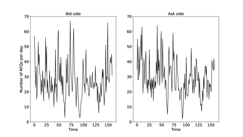
Figure 1: Number of RFQs per day at the bid and at the ask for Sector 1.

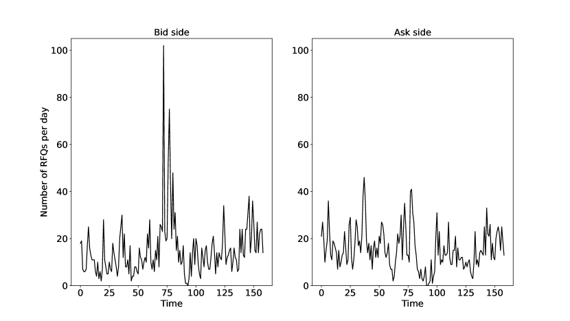
Figure 2: Number of RFQs per day at the bid and at the ask for Sector 2.

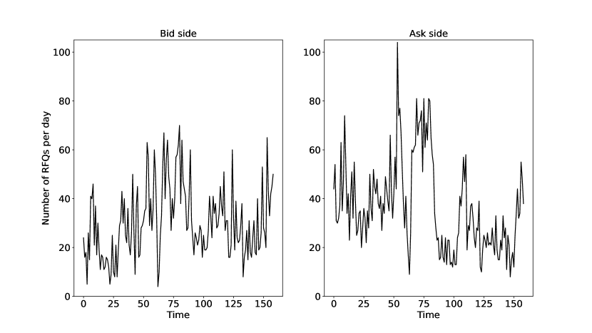
Figure 3: Number of RFQs per day at the bid and at the ask for Sector 3.

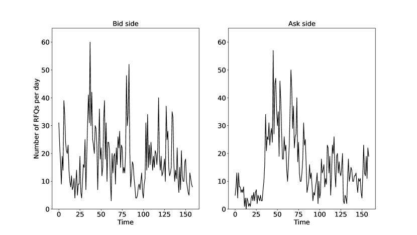
Figure 4: Number of RFQs per day at the bid and at the ask for Sector 4.

Sector	$\lambda^{1}$	$\lambda^{2}$	$Q$
Sector 1	10.83	73.03	$\begin{pmatrix}-14.01&4.37&4.37&5.27\\ 19.32&-60.91&12.54&29.05\\ 19.32&12.54&-60.91&29.05\\ 23.67&15.00&15.00&-53.67\end{pmatrix}$
Sector 2	8.44	58.28	$\begin{pmatrix}-4.55&1.00&1.00&2.55\\ 18.53&-28.31&0.13&9.65\\ 18.53&0.13&-28.31&9.65\\ 14.77&16.73&16.73&-48.23\end{pmatrix}$
Sector 3	15.73	81.78	$\begin{pmatrix}-9.98&2.79&2.79&4.40\\ 20.53&-23.73&0.02&3.18\\ 20.53&0.02&-23.73&3.18\\ 9.87&4.17&4.17&-18.21\end{pmatrix}$
Sector 4	7.33	28.32	$\begin{pmatrix}-1.67&0.48&0.48&0.71\\ 1.92&-2.02&0.00&0.10\\ 1.92&0.00&-2.02&0.10\\ 0.84&0.11&0.11&-1.06\end{pmatrix}$

Table 1: Estimated parameters of the Markov-modulated Poisson process for the four sectors.

Once the parameters of the MMPPs have been estimated, we can evaluate at each point in time the probability to be in each state (see Section 2.2.3). In Figures 5, 6, 7 and 8, we document the distribution of the values taken by the probability $\pi^{0,1}$ (resp. $\pi^{1,0}$) to be in a low/high-liquidity (resp. high/low-liquidity) state. We clearly see that high values of these probabilities are quite rare: it is hard to be certain that a desquilibrium in RFQs indeed corresponds to an underlying asymmetric regime.

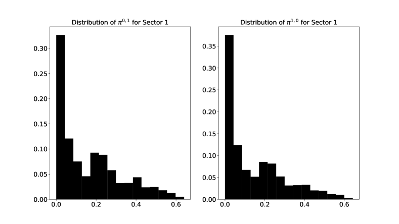
Figure 5: Distribution of the values taken by $\pi^{0,1}$ and $\pi^{1,0}$ for Sector 1.

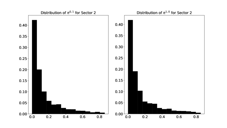
Figure 6: Distribution of the values taken by $\pi^{0,1}$ and $\pi^{1,0}$ for Sector 2.

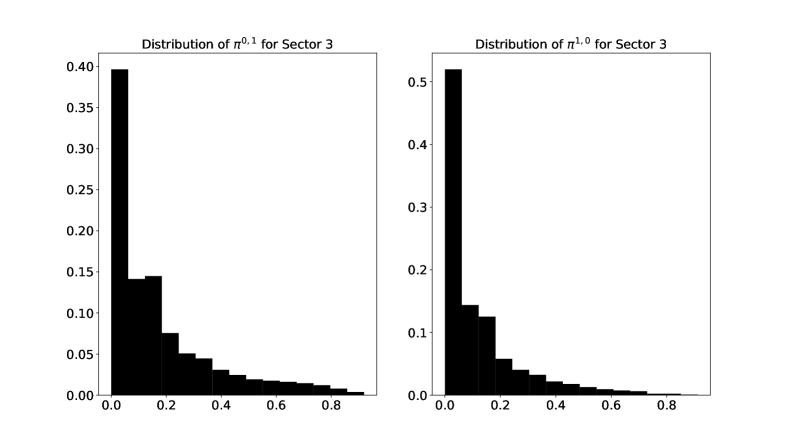
Figure 7: Distribution of the values taken by $\pi^{0,1}$ and $\pi^{1,0}$ for Sector 3.

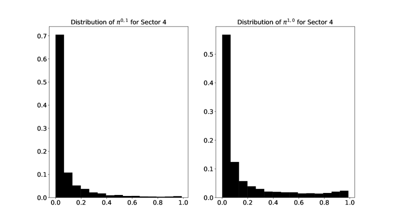
Figure 8: Distribution of the values taken by $\pi^{0,1}$ and $\pi^{1,0}$ for Sector 4.

4.3 Micro-price

4.3.1 Estimation of $\kappa$

In order to illustrate our concept of micro-price, we need first to estimate the parameter $\kappa$ in the dynamics of bond prices. For each sector, we consider 4 bonds amongst those available in the database. We first compute the functions $v$ given by Eq. (3) and then use Eq. (4) to perform a linear regression and estimate $\kappa$ for each bond. We also compute the arithmetic volatility $\sigma$ and the weight $\beta$ associated with each bond (see Section 2.3.2). The results are reported in Table 2.

The estimated values for $\kappa$ are not all significantly different for $0$ (given the standard deviations reported), but it is nevertheless interesting to notice that the figures are positive for all bonds. This tends to prove that imbalance in the flow of RFQs has a consistant predictive power on the variation of the price, hence the interest of the concept of micro-price.

4.3.2 Micro-price in practice

In Table 3, we took the last composite mid-price and bid-ask spread in the dataset for each of the 16 bonds we focus on, and computed the corresponding micro-price when we are $100\%$ sure that the market is imbalanced, one way or the other.

Of course, and this is confirmed by the above histograms, one can seldom be certain to be in any of the two imbalanced states. In practice, the micro-price must therefore be computed as an expectation over the different possible states, i.e. as a function of the current estimates of the probabilities to be in each state. In particular, the micro-prices exhibited in Table 3 correspond to theoretical bounds for the micro-price that would be used in practice.

Sector	Bond	$\beta$	$\kappa$ (stdev)	$\sigma$
1	1	0.10	2.29 (0.55)	18.39
	2	0.10	0.25 (0.49)	15.43
	3	0.06	2.83 (1.66)	22.55
	4	0.05	0.33 (2.23)	19.75
2	1	0.19	0.57 (0.19)	13.75
	2	0.14	0.90 (0.22)	16.05
	3	0.11	0.65 (0.16)	9.80
	4	0.10	0.86 (0.68)	20.36
3	1	0.11	0.61 (0.34)	9.93
	2	0.09	0.05 (0.16)	18.41
	3	0.06	0.11 (0.08)	12.23
	4	0.05	0.08 (0.11)	18.68
4	1	0.21	0.04 (0.02)	13.00
	2	0.12	0.01 (0.01)	24.09
	3	0.12	0.08 (0.04)	16.91
	4	0.07	0.09 (0.05)	12.67

Table 2: Estimations of $\beta$, $\kappa$ and $\sigma$.

Sector	Bond	Mid-price	Bid price	Ask price	Micro-price $\pi^{1,0}\!\!\!=\!\!1$	Micro-price $\pi^{0,1\!}\!\!=\!\!1$
1	1	103.593	103.098	104.088	101.652	105.534
	2	97.107	96.614	97.600	96.892	97.322
	3	99.146	98.631	99.661	96.752	101.541
	4	94.187	93.049	95.325	93.909	94.465
2	1	99.823	99.291	100.355	98.819	100.827
	2	99.270	98.603	99.936	97.700	100.840
	3	99.649	98.815	100.483	98.513	100.784
	4	98.903	97.570	100.235	97.970	99.835
3	1	95.338	94.674	96.001	93.634	97.041
	2	92.394	91.860	92.927	92.252	92.535
	3	97.137	96.484	97.790	96.819	97.455
	4	94.839	94.220	95.458	94.810	94.867
4	1	102.632	102.151	103.112	102.252	103.011
	2	104.785	104.327	105.242	104.717	104.853
	3	104.824	104.293	105.355	103.994	105.654
	4	108.438	107.991	108.884	107.500	109.375

Table 3: Micro-price for the different bonds in imbalanced states.

In what follows, we study how the micro-price evolves depending on the probabilities of the different states of the MMPP, for the first bond of each sector. Notice that, in our case, the respective values of $\pi^{0,0}$ and $\pi^{1,1}$ have no impact on the micro-price: only $\pi^{0,1}$ and $\pi^{1,0}$ matter.

In Figure 9, we plot the micro-price as a function of $\pi^{0,1}$, when $\pi^{1,0}=0.$ Figure 10 documents similarly the micro-price as a function of $\pi^{0,1}$, when $\pi^{1,0}=0.3$. To study the impact of the uncertainty on the parameter $\kappa$, we also plot the micro-prices corresponding to values of $\kappa$ one standard deviation above and below our estimation. Composite bid-ask spreads are also reported in the Figures.

Naturally, when $\pi^{0,1}=\pi^{1,0}$, the micro-price is equal to the mid-price. As expected, we also see that a rise in $\pi^{0,1}$ leads to an increase in micro-prices. In Figure 9, we see that micro-prices are within the composite bid-ask spread for moderate values of $\pi^{0,1}$ but beyond for large values (except for Bond 4.1). Values beyond the bid-ask spread could be seen as a real trading signal, but it is important to have in mind that the results obtained for high values of $\pi^{0,1}$ have to be taken with care because the linear regressions have been carried out with only a few high values for $\pi^{0,1}$ (see the above histograms). We see in Figure 10 that when $\pi^{1,0}=0.3$, most values remain inside the bid-ask spread. In fact, we see in Figures 11, 12, 13 and 14 that micro-prices are significantly outside of the bid-ask spread for extreme values of $\pi^{0,1}$ and $\pi^{1,0}$ (in opposite directions) only, i.e. when one is really sure that the flow is imbalanced.

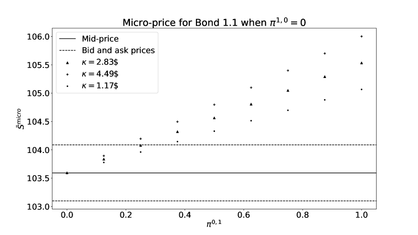
(a) Bond 1.1

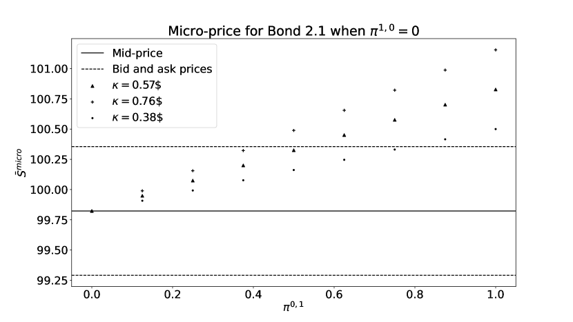
(b) Bond 2.1

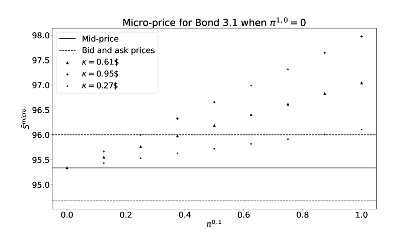
(c) Bond 3.1

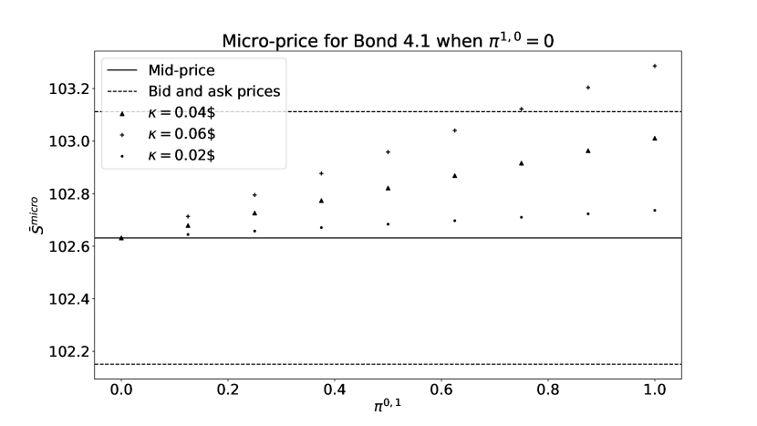
(d) Bond 4.1

Figure 9: Micro-price for different bonds as a function of $\pi^{0,1}$ when $\pi^{1,0}=0$.

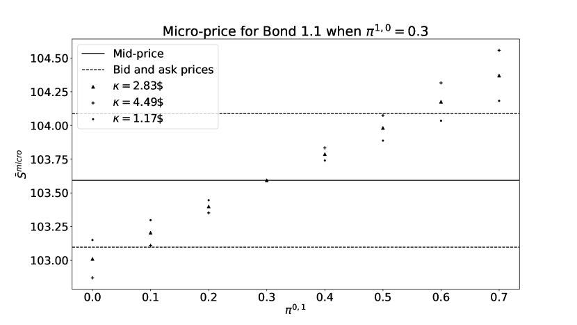
(a) Bond 1.1

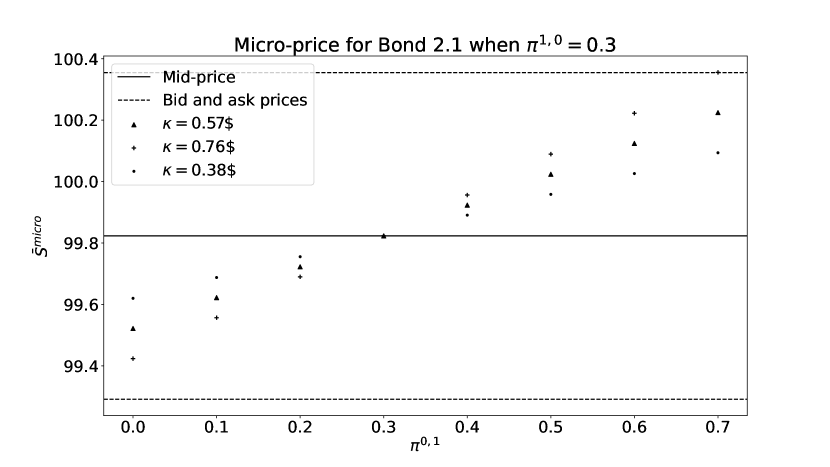
(b) Bond 2.1

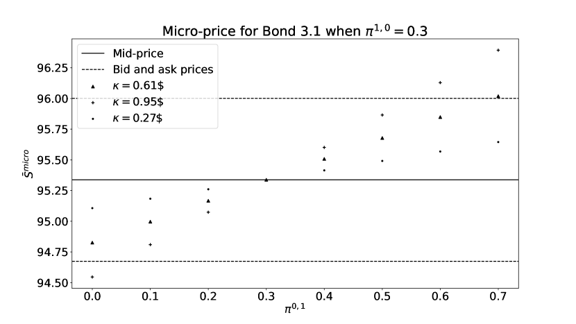
(c) Bond 3.1

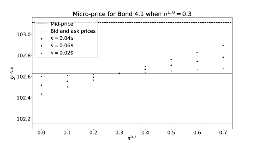
(d) Bond 4.1

Figure 10: Micro-price for different bonds as a function of $\pi^{0,1}$ when $\pi^{1,0}=0.3$.

Figure 11: Micro-price for Bond 1.1 as a function of $\pi^{0,1}$ and $\pi^{1,0}$.

Figure 12: Micro-price for Bond 2.1 as a function of $\pi^{0,1}$ and $\pi^{1,0}$.

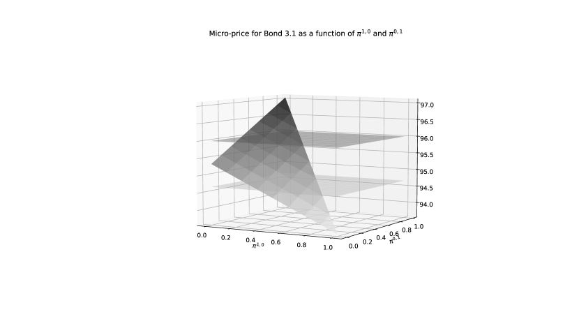
Figure 13: Micro-price for Bond 3.1 as a function of $\pi^{0,1}$ and $\pi^{1,0}$.

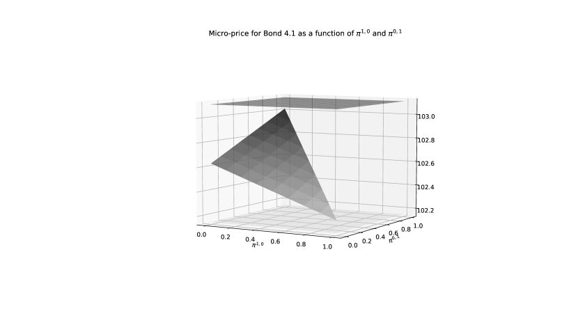
Figure 14: Micro-price for Bond 4.1 as a function of $\pi^{0,1}$ and $\pi^{1,0}$.

4.4 Fair Transfer Price

Let us now come to the case of Fair Transfer Prices. For that purpose, we need to fit S-curves, choose a risk aversion parameter and solve a HJB equation.

4.4.1 Estimation of S-curves

For the functions $f^{b}$ and $f^{a}$ defined in Section 3.2.1, we assume a logistic form. We noticed no systematic difference between the bid and ask sides. Consequently, we considered

$$f^{b}(\delta)=f^{a}(\delta)=\frac{1}{1+e^{\alpha+\frac{\beta}{\delta^{0}}\delta}}=:f(\delta),$$

where $\delta^{0}$ is the current composite bid-ask spread of the bond, and the parameters $\alpha$ and $\beta$ are estimated with a logistic regression.

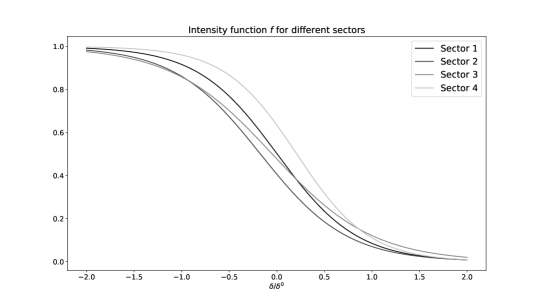
Figure 15: Intensity function $f$ for the different sectors.

With this parametrization, the functions appeared to be almost uniform accross sectors (as shown in Figure 15), and we therefore estimated, for the sake of simplicity, a single S-curve using the entire dataset, independently of the sector. We obtained the following (rounded) values: $\alpha=-0.7$ and $\beta=3.1$.

4.4.2 Solving HJB equations

Our concept of FTP relies on the bid and ask quotes of a theoretical market maker that knows the current state of the market. To solve the stochastic optimal control problem of that market maker and obtain the associated quotes, one needs to compute numerically the value functions.

Let us recall that, in the model of Section 3, the value functions $(\theta^{j_{b},j_{a}})_{1\leq j_{b}\leq m_{b},1\leq j_{a}\leq m_{a}}$ of the market maker satisfy the following system of Hamilton-Jacobi-Bellman (HJB) equations:

$$\partial_{t}\theta^{j_{b},j_{a}}(t,q)+\kappa(\lambda^{j_{a},a}-\lambda^{j_{b},b})q-\frac{1}{2}\gamma\sigma^{2}q^{2}+\sum_{1\leq k_{b}\leq m_{b},1\leq k_{a}\leq m_{a}}Q_{(j_{b}-1)m_{a}+j_{a},(k_{b}-1)m_{a}+k_{a}}\theta^{k_{b},k_{a}}(t,q)$$

$$+z\lambda^{j_{b},b}H^{b}\left(\frac{\theta^{j_{b},j_{a}}(t,q)-\theta^{j_{b},j_{a}}(t,q+z)}{z}\right)+z\lambda^{j_{a},a}H^{a}\left(\frac{\theta^{j_{b},j_{a}}(t,q)-\theta^{j_{b},j_{a}}(t,q-z)}{z}\right)=0$$

with terminal condition $\theta^{j_{b},j_{a}}(T,q)=0$.

We need to compute or approximate numerically the solution of this system of equations in order to compute FTPs. A natural approach is to use a Euler scheme, preferably implicit. In that case, relevant boundary conditions can be chosen by adding risk limits to the inventory of the theoretical market maker, and the equations become

$$\partial_{t}\theta^{j_{b},j_{a}}(t,q)+\kappa(\lambda^{j_{a},a}-\lambda^{j_{b},b})q-\frac{1}{2}\gamma\sigma^{2}q^{2}+\sum_{1\leq k_{b}\leq m_{b},1\leq k_{a}\leq m_{a}}Q_{(j_{b}-1)m_{a}+j_{a},(k_{b}-1)m_{a}+k_{a}}\theta^{k_{b},k_{a}}(t,q)$$

$$+z\lambda^{j_{b},b}\mathds{1}_{\{q+z\leq\bar{q}\}}H^{b}\left(\frac{\theta^{j_{b},j_{a}}(t,q)-\theta^{j_{b},j_{a}}(t,q+z)}{z}\right)+z\lambda^{j_{a},a}\mathds{1}_{\{q-z\geq-\bar{q}\}}H^{a}\left(\frac{\theta^{j_{b},j_{a}}(t,q)-\theta^{j_{b},j_{a}}(t,q-z)}{z}\right)=0$$

with terminal condition $\theta^{j_{b},j_{a}}(T,q)=0$, where $\bar{q}>0$ corresponds to the risk limit, i.e. the market maker refuses any trade that would bring the inventory out of the interval $[-\bar{q},\bar{q}]$. If $\bar{q}$ is large enough, this has almost no impact on the bid and ask quotes of the market maker at $q=0$ that are used to compute FTPs.

Euler schemes can be time-consuming when the number of states $m_{b}\times m_{a}$ is large, or even unfeasible if the one-asset market making model is replaced by a multi-asset one. Using the same approach as in [6], we propose in the following paragraphs a quadratic approximation of the value functions.

Let us replace the Hamiltonian functions $H^{b}$ and $H^{a}$ by the quadratic functions

$$\check{H}^{b}:p\mapsto\alpha^{b}_{0}+\alpha^{b}_{1}p+\frac{1}{2}\alpha^{b}_{2}p^{2}\quad\textrm{and}\quad\check{H}^{a}:p\mapsto\alpha^{a}_{0}+\alpha^{a}_{1}p+\frac{1}{2}\alpha^{a}_{2}p^{2}.$$

A natural choice for the functions $\check{H}^{b}$ and $\check{H}^{a}$ derives from Taylor expansions around $p=0$. In that case, we have

$$\forall i\in\{0,1,2\},\quad\alpha^{b}_{i}={H^{b}}^{(i)}(0)\quad\textrm{and}\quad\alpha^{a}_{i}={H^{a}}^{(i)}(0).$$

For $(j_{b},j_{a})\in\{1,\ldots,m_{b}\}\times\{1,\ldots,m_{a}\}$, we denote by $\check{\theta}^{j_{b},j_{a}}$ the approximation of $\theta^{j_{b},j_{a}}$ associated with the functions $\check{H}^{b}$ and $\check{H}^{a}$. The functions $(\check{\theta}^{j_{b},j_{a}})_{1\leq j_{b}m_{b},1\leq j_{a}\leq m_{a}}$ verify

$$0 = \partial_{t}\check{\theta}^{j_{b},j_{a}}(t,q)+\kappa(\lambda^{j_{a},a}-\lambda^{j_{b},b})q-\frac{1}{2}\gamma\sigma^{2}q^{2}$$

$$+\sum_{1\leq k_{b}\leq m_{b},1\leq k_{a}\leq m_{a}}Q_{(j_{b}-1)m_{a}+j_{a},(k_{b}-1)m_{a}+k_{a}}\check{\theta}^{k_{b},k_{a}}(t,q)+z\left(\lambda^{j_{b},b}\alpha^{b}_{0}+\lambda^{j_{a},a}\alpha^{a}_{0}\right)$$

$$+\left(\lambda^{j_{b},b}\alpha^{b}_{1}\left(\check{\theta}^{j_{b},j_{a}}(t,q)-\check{\theta}^{j_{b},j_{a}}(t,q+z)\right)+\lambda^{j_{a},a}\alpha^{a}_{1}\left(\check{\theta}^{j_{b},j_{a}}(t,q)-\check{\theta}^{j_{b},j_{a}}(t,q-z)\right)\right)$$

$$+\frac{1}{2z}\left(\lambda^{j_{b},b}\alpha^{b}_{2}\left(\check{\theta}^{j_{b},j_{a}}(t,q)-\check{\theta}^{j_{b},j_{a}}(t,q+z)\right)^{2}+\lambda^{j_{a},a}\alpha^{a}_{2}\left(\check{\theta}^{j_{b},j_{a}}(t,q)-\check{\theta}^{j_{b},j_{a}}(t,q-z)\right)^{2}\right),$$

and of course we consider the terminal condition $\check{\theta}^{j_{b},j_{a}}(T,q)=0$.

To write the approximations of the value functions in a simple way, let us introduce for $i\in\{0,1,2\}$ and $k\in\mathbb{N}$

$$\Delta_{i,k}^{b}=\alpha^{b}_{i}z^{k}\quad\text{and}\quad\Delta_{i,k}^{a}=\alpha^{a}_{i}z^{k}.\vspace{-0.1cm}$$

For $(j_{b},j_{a})\in\{1,\ldots,m_{b}\}\times\{1,\ldots,m_{a}\}$, let us consider three differentiable functions $A_{j_{b},j_{a}}:[0,T]\to\mathbb{R}$, $B_{j_{b},j_{a}}:[0,T]\to\mathbb{R}$, and $C_{j_{b},j_{a}}:[0,T]\to\mathbb{R}$ solutions of the system of ordinary differential equations

$$\begin{cases}\displaystyle{A_{j_{b},j_{a}}^{\prime}}(t)=&2\left(\lambda^{j_{b},b}\Delta^{b}_{2,1}+\lambda^{j_{a},a}\Delta^{a}_{2,1}\right)A_{j_{b},j_{a}}(t)^{2}-\frac{1}{2}\gamma\sigma^{2}\\ &-\sum_{1\leq k_{b}\leq m_{b},1\leq k_{a}\leq m_{a}}Q_{(j_{b}-1)m_{a}+j_{a},(k_{b}-1)m_{a}+k_{a}}A_{k_{b},k_{a}}(t)\\ {B_{j_{b},j_{a}}^{\prime}}(t)=&2\left(\lambda^{j_{b},b}\Delta^{b}_{1,1}-\lambda^{j_{a},a}\Delta^{a}_{1,1}\right)A_{j_{b},j_{a}}(t)+2\left(\lambda^{j_{b},b}\Delta^{b}_{2,2}-\lambda^{j_{a},a}\Delta^{a}_{2,2}\right)A_{j_{b},j_{a}}(t)^{2}\\ &+\kappa(\lambda^{j_{a},a}-\lambda^{j_{b},b})+2\left(\lambda^{j_{b},b}\Delta^{b}_{2,1}+\lambda^{j_{a},a}\Delta^{a}_{2,1}\right)A_{j_{b},j_{a}}(t)B_{j_{b},j_{a}}(t)\\ &-\sum_{1\leq k_{b}\leq m_{b},1\leq k_{a}\leq m_{a}}Q_{(j_{b}-1)m_{a}+j_{a},(k_{b}-1)m_{a}+k_{a}}B_{k_{b},k_{a}}(t)\\ {C_{j_{b},j_{a}}^{\prime}}(t)=&\left(\lambda^{j_{b},b}\Delta^{b}_{0,1}+\lambda^{j_{a},a}\Delta^{a}_{0,1}\right)+\left(\lambda^{j_{b},b}\Delta^{b}_{1,2}+\lambda^{j_{a},a}\Delta^{a}_{1,2}\right)A_{j_{b},j_{a}}(t)\\ &+\left(\lambda^{j_{b},b}\Delta^{b}_{1,1}-\lambda^{j_{a},a}\Delta^{a}_{1,1}\right)B_{j_{b},j_{a}}(t)+\frac{1}{2}\left(\lambda^{j_{b},b}\Delta^{b}_{2,3}+\lambda^{j_{a},a}\Delta^{a}_{2,3}\right)A_{j_{b},j_{a}}(t)^{2}\\ &+\frac{1}{2}\left(\lambda^{j_{b},b}\Delta^{b}_{2,1}+\lambda^{j_{a},a}\Delta^{a}_{2,1}\right)B_{j_{b},j_{a}}(t)^{2}+\left(\lambda^{j_{b},b}\Delta^{b}_{2,2}-\lambda^{j_{a},a}\Delta^{a}_{2,2}\right)A_{j_{b},j_{a}}(t)B_{j_{b},j_{a}}(t)\\ &-\sum_{1\leq k_{b}\leq m_{b},1\leq k_{a}\leq m_{a}}Q_{(j_{b}-1)m_{a}+j_{a},(k_{b}-1)m_{a}+k_{a}}C_{k_{b},k_{a}}(t),\end{cases}$$

with terminal conditions $A_{j_{b},j_{a}}(T)=0$, $B_{j_{b},j_{a}}(T)=0$ and $C_{j_{b},j_{a}}(T)=0$.

Then, for all $(j_{b},j_{a})\in\{1,\ldots,m_{b}\}\times\{1,\ldots,m_{a}\}$, we have:

$$\check{\theta}^{j_{b},j_{a}}(t,q)=-q^{2}A_{j_{b},j_{a}}(t)-qB_{j_{b},j_{a}}(t)-C_{j_{b},j_{a}}(t).\vspace{-0.1cm}$$

Moreover, asymptotic results on value functions continue to hold on their approximations.

This kind of approximations has been used in [4, 5] with great success in terms of risk management. We investigate the quality of the approximation in terms of FTPs below.

4.4.3 FTP in practice

To compute FTPs as proposed in Section 3.2.1, we still have to choose the risk aversion of the theoretical market maker. A natural way to choose $\gamma$ is to calibrate it to composite bid and ask prices, i.e. we assume that the quotes of the theoretical market maker correspond to that of the market when inventory is equal to $0$.

The optimal strategy of the theoretical market maker is obtained by solving numerically the HJB equation, using an implicit Euler scheme, and through a quadratic approximation of the value function. Depending on the numerical method we use, $\gamma$ calibrated to composite bid and ask prices takes different values. However, in terms of FTP, the results obtained with the two numerical methods are almost identical, as shown in Table 4 (FTP (a) corresponds to the Euler scheme and FTP (b) to the quadratic approximation). As for micro-prices, in practice, one can never be certain to be in any given state, and the FTP has to be computed as an expectation over the different possible states, depending on the current estimate. Therefore the FTPs exhibited in Table 4 correspond to bounds for the FTPs that would be used in practice. Notice that the adjustments given by FTPs are of lower magnitude than those suggested by micro-prices. As for micro-prices, we study how FTPs evolve depending on the probabilities. Figure 16 documents FTPs as a function of $\pi^{0,1}$, when $\pi^{1,0}=0$ while Figure 17 documents FTPs as a function of $\pi^{0,1}$, when $\pi^{1,0}=0.3$. We see that adjustments are always small. This is linked to the fact that, even when the market is imbalanced, market makers can slightly skew their quotes to deter risk-increasing trades and transform requests into trades when trades would result in a less risky position (less inventory in absolute value in our case). This strongly relies on our implicit assumption that S-curves are the same independently of the liquidity regime. However, we found no empirical evidence of the influence of intensities on fill rates.

Bond	$\gamma$ (a)	$\gamma$ (b)	Bid price	Ask price	$\pi^{\!1,0}\!\!=\!\!1\!\!\!$ : FTP (a)	FTP (b)	$\pi^{\!0,1}\!\!=\!\!1\!\!\!$ : FTP (a)	FTP (b)
1.1	$4.5\cdot 10^{-9}$	$5.1\cdot 10^{-9}$	103.098	104.088	103.458	103.458	103.728	103.729
1.2	$8.9\cdot 10^{-9}$	$9.1\cdot 10^{-9}$	96.514	97.600	97.092	97.092	97.122	97.122
1.3	$4.4\cdot 10^{-8}$	$5.2\cdot 10^{-8}$	98.631	99.661	99.038	99.037	99.254	99.255
1.4	$8.5\cdot 10^{-7}$	$1.6\cdot 10^{-6}$	93.049	95.325	94.167	94.172	94.207	94.202
2.1	$6.1\cdot 10^{-8}$	$6.9\cdot 10^{-8}$	99.291	100.355	99.682	99.681	99.964	99.965
2.2	$7.0\cdot 10^{-8}$	$8.3\cdot 10^{-8}$	98.603	99.936	99.106	99.104	99.433	99.435
2.3	$1.1\cdot 10^{-7}$	$1.2\cdot 10^{-7}$	98.815	100.483	99.554	99.553	99.743	99.744
2.4	$1.3\cdot 10^{-7}$	$1.6\cdot 10^{-7}$	97.570	100.235	98.824	98.824	98.981	98.981
3.1	$4.9\cdot 10^{-7}$	$5.6\cdot 10^{-7}$	94.674	96.001	95.195	95.193	95.480	95.482
3.2	$6.1\cdot 10^{-7}$	$7.6\cdot 10^{-7}$	91.860	92.927	92.364	92.365	92.423	94.422
3.3	$7.0\cdot 10^{-7}$	$9.6\cdot 10^{-7}$	96.484	97.790	97.104	97.107	97.169	97.166
3.4	$4.3\cdot 10^{-7}$	$7.7\cdot 10^{-7}$	94.220	95.458	94.815	94.824	94.860	94.851
4.1	$1.2\cdot 10^{-7}$	$1.3\cdot 10^{-7}$	102.151	103.112	102.523	102.525	102.740	102.738
4.2	$1.3\cdot 10^{-7}$	$1.7\cdot 10^{-7}$	104.327	105.242	104.691	104.701	104.878	104.868
4.3	$1.8\cdot 10^{-7}$	$2.2\cdot 10^{-7}$	104.293	105.355	104.697	104.706	104.951	104.942
4.4	$1.5\cdot 10^{-8}$	$1.6\cdot 10^{-8}$	107.991	108.884	108.377	108.377	108.498	108.498

Table 4: FTP for the different bonds in imbalanced states.

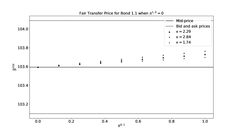
(a) Bond 1.1

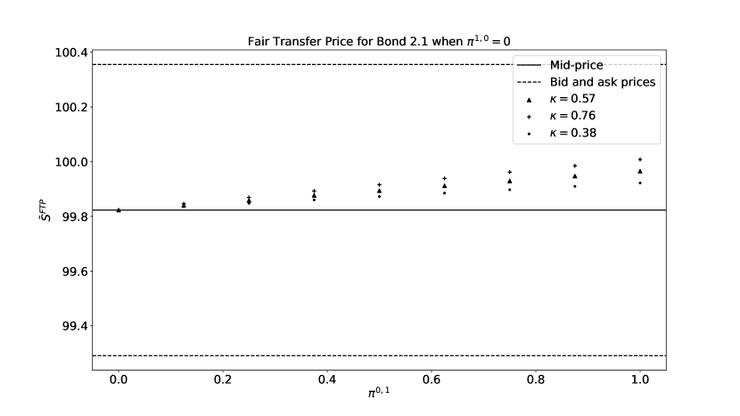
(b) Bond 2.1

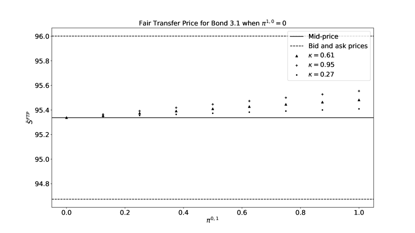
(c) Bond 3.1

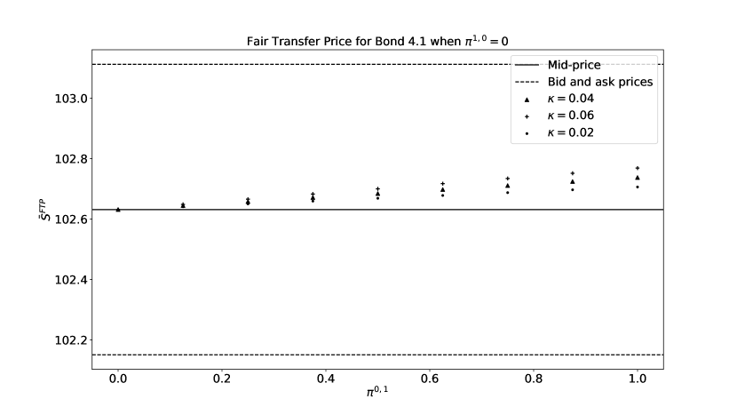
(d) Bond 4.1

Figure 16: FTP for different bonds as a function of $\pi^{0,1}$ when $\pi^{1,0}=0$.

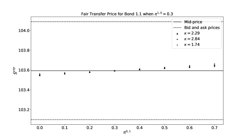
(a) Bond 1.1

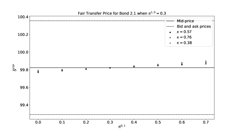
(b) Bond 2.1

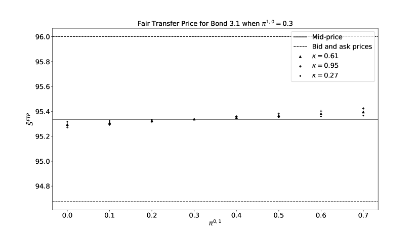
(c) Bond 3.1

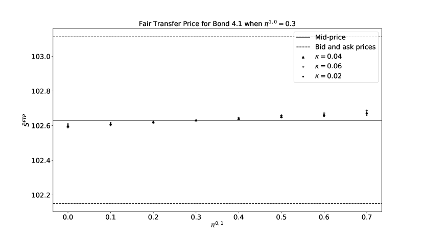
(d) Bond 4.1

Figure 17: FTP for different bonds as a function of $\pi^{0,1}$ when $\pi^{1,0}=0.3$.

Conclusion

In this paper, we developed a new approach to model liquidity in corporate bond markets. This approach, which can be used in any OTC market where clients request dealers for prices, relies on Markov-modulated Poisson processes. The statistical estimation procedure we proposed is based on an EM algorithm and can be used either at the bond level or at a more macroscopic level (at the sector level for instance). Although asymmetric states are hard to identify with great confidence, we showed that flow imbalances contain information about the evolution of the price and use flow asymmetries to generalize the notion of micro-price proposed by Stoikov in the context of markets organized around limit order books. We also coined a new concept inspired by the recent market making literature: Fair Transfer Price. It is related to the quotes proposed by a market maker who takes flow imbalances into account and therefore projects liquidity asymmetries onto the price space. We noticed that the price adjustments associated with FTP are often small, smaller than those associated with micro-prices.

Data availability statement

Due to confidentiality reasons, the data used in this article cannot be made publicly available.

References

- [1] Marco Avellaneda and Sasha Stoikov. High-frequency trading in a limit order book. Quantitative Finance, 8(3):217–224, 2008.
- [2] Bastien Baldacci, Philippe Bergault, Joffrey Derchu, and Mathieu Rosenbaum. On bid and ask side-specific tick sizes. to appear in SIAM Journal on Financial Mathematics, 2024.
- [3] Alexander Barzykin, Philippe Bergault, and Olivier Guéant. Algorithmic market making in dealer markets with hedging and market impact. Mathematical Finance, 33(1):41–79, 2023.
- [4] Alexander Barzykin, Philippe Bergault, and Olivier Guéant. Market making by an foreign exchange dealer. Risk Magazine, August 2022.
- [5] Alexander Barzykin, Philippe Bergault, and Olivier Guéant. Dealing with multi-currency inventory risk in foreign exchange cash markets. Risk Magazine, March 2023.
- [6] Philippe Bergault, David Evangelista, Olivier Guéant, and Douglas Vieira. Closed-form approximations in multi-asset market making. Applied Mathematical Finance, 28(2):101–142, 2021.
- [7] Philippe Bergault and Olivier Guéant. Size matters for otc market makers: general results and dimensionality reduction techniques. Mathematical Finance, 31(1):279–322, 2021.
- [8] Julius Bonart and Fabrizio Lillo. A continuous and efficient fundamental price on the discrete order book grid. Physica A: Statistical Mechanics and its Applications, 503:698–713, 2018.
- [9] Alvaro Cartea, Ryan Donnelly, and Sebastian Jaimungal. Enhancing trading strategies with order book signals. Applied Mathematical Finance, 25(1):1–35, 2018.
- [10] Álvaro Cartea, Sebastian Jaimungal, and José Penalva. Algorithmic and high-frequency trading. Cambridge University Press, 2015.
- [11] Álvaro Cartea, Sebastian Jaimungal, and Jason Ricci. Buy low, sell high: A high frequency trading perspective. SIAM Journal on Financial Mathematics, 5(1):415–444, 2014.
- [12] Rama Cont and Adrien De Larrard. Price dynamics in a Markovian limit order market. SIAM Journal on Financial Mathematics, 4(1):1–25, 2013.
- [13] Khalil Dayri and Mathieu Rosenbaum. Large tick assets: implicit spread and optimal tick size. Market Microstructure and Liquidity, 1(01):1550003, 2015.
- [14] Sylvain Delattre, Christian Y. Robert, and Mathieu Rosenbaum. Estimating the efficient price from the order flow: a Brownian Cox process approach. Stochastic Processes and their Applications, 123(7):2603–2619, 2013.
- [15] Jens Dick-Nielsen. Liquidity biases in TRACE. The Journal of Fixed Income, 19(2):43–55, 2009.
- [16] Jens Dick-Nielsen. How to clean enhanced TRACE data. Available at SSRN 2337908, 2014.
- [17] Wolfgang Fischer and Kathleen Meier-Hellstern. The markov-modulated poisson process (mmpp) cookbook. Performance evaluation, 18(2):149–171, 1993.
- [18] Lawrence R. Glosten and Paul R. Milgrom. Bid, ask and transaction prices in a specialist market with heterogeneously informed traders. Journal of financial economics, 14(1):71–100, 1985.
- [19] Martin D. Gould and Julius Bonart. Queue imbalance as a one-tick-ahead price predictor in a limit order book. Market Microstructure and Liquidity, 2(02):1650006, 2016.
- [20] Olivier Guéant, Charles-Albert Lehalle, and Joaquin Fernandez-Tapia. Dealing with the inventory risk: a solution to the market making problem. Mathematics and financial economics, 7(4):477–507, 2013.
- [21] Olivier Guéant and Jiang Pu. Mid-price estimation for European corporate bonds: a particle filtering approach. Market microstructure and liquidity, 4(01n02):1950005, 2018.
- [22] Olivier Guéant. The Financial Mathematics of Market Liquidity: From optimal execution to market making, volume 33. CRC Press, 2016.
- [23] Olivier Guéant. Optimal market making. Applied Mathematical Finance, 24(2):112–154, 2017.
- [24] Olivier Guéant and Iuliia Manziuk. Optimal control on graphs: existence, uniqueness, and long-term behavior. ESAIM: Control, Optimisation and Calculus of Variations, 26:22, 2020.
- [25] Thibault Jaisson. Liquidity and impact in fair markets. Market Microstructure and Liquidity, 1(02):1550010, 2015.
- [26] Charles-Albert Lehalle and Othmane Mounjid. Limit order strategic placement with adverse selection risk and the role of latency. Market Microstructure and Liquidity, 3(01):1750009, 2017.
- [27] Ananth Madhavan, Matthew Richardson, and Mark Roomans. Why do security prices change? A transaction-level analysis of NYSE stocks. The Review of Financial Studies, 10(4):1035–1064, 1997.
- [28] Kathleen S Meier-Hellstern. A fitting algorithm for markov-modulated poisson processes having two arrival rates. European Journal of Operational Research, 29(3):370–377, 1987.
- [29] Roel Oomen. Last look. Quantitative Finance, 17(7):1057–1070, 2017.
- [30] Christian Y. Robert and Mathieu Rosenbaum. A new approach for the dynamics of ultra-high-frequency data: The model with uncertainty zones. Journal of Financial Econometrics, 9(2):344–366, 2011.
- [31] Tobias Rydén. An EM algorithm for estimation in Markov-modulated Poisson processes. Computational Statistics & Data Analysis, 21(4):431–447, 1996.
- [32] Sasha Stoikov. The micro-price: a high-frequency estimator of future prices. Quantitative Finance, 18(12):1959–1966, 2018.
- [33] Sasha Stoikov, Peter Decrem, Yikai Hua, and Anne Shen. The Microstructure of Cointegrated Assets. Available at SSRN 3824298, 2021.