Symmetry-Enriched Criticality in a Coupled Spin-Ladder
Abstract
We study a one-dimensional ladder of two coupled XXZ spin chains and identify several distinct gapless symmetry-enriched critical phases. These have the same unbroken symmetries and long-wavelength description, but cannot be connected without encountering either a phase transition or other intermediate phases. Using bosonizaion, we analyze the nature of their distinction by determining how microscopic symmetries are manifested in the long-wavelength fields, the behavior of charged local and nonlocal operators, and identify the universality class of all direct continuous phase transitions between them. One of these phases is a gapless topological phase with protected edge modes. We characterize its precise nature and place it within the broader classification. We also find the occurrence of ‘multiversality’ in the phase diagram, wherein two fixed phases are separated by continuous transitions with different universality classes in different parameter regimes. We determine the phase diagram and all its aspects, as well as verify our predictions numerically using density matrix renormalization group and a mapping onto an effective spin-1 model.
I Introduction
One of the most remarkable characteristics of quantum and classical many-body physical systems is the emergence of distinct, stable phases that are divided by sharp phase transitions. There is tremendous theoretical and experimental interest in enumerating all possible phases and transitions and characterizing their properties. Symmetries have provided a guiding principle to facilitate this. It was realized that distinct phases of matter occur when microscopic symmetries are spontaneously broken at long distances [1]. The knowledge of microscopic symmetries allows us to enumerate the different ways it can be spontaneously broken, the properties of the resulting long-range order, and sometimes even the nature of the phase transition. The concept of ‘topological’ ordering that falls outside the symmetry-breaking framework [2] following the discovery of the quantum Hall effect [3] has expanded the mechanisms by which distinct phases can arise. This has spurred a flurry of intense research activity over the past decades in classifying and characterizing gapped phases of matter [4]. These new phases represent multiple ways in which symmetries can be unbroken and yet result in different phases. The distinguishing features are detectable in subtle signatures present in entanglement patterns and boundary/ topology effects.
Gapless phases, on the other hand, have been left by the wayside in these recent developments. Despite being ubiquitous in nature and making frequent appearances in the phase diagrams of many known physical systems, the mechanisms by which they arise and are stabilized are relatively unclear although various descriptive frameworks have been successfully devised to understand them. For example, when noninteracting bands of fermions are partially filled they lead to the formation of Fermi liquids [5], Dirac [6] / Weyl [7] semimetals. Using partons and emergent gauge fields to describe systems has also been useful in accessing non-Fermi-liquid phases [8, 9]. The most systematic known mechanism is arguably the spontaneous breaking of continuous symmetries, e.g., which results in the formation of superfluids. The program of classifying gapless states of matter with unbroken symmetries is still in its early stages.
Examples of gapless states hosting edge modes have been reported in various works [10, 11, 12, 13, 14, 15, 16, 17, 18, 19] and was developed into the notion of gapless symmetry protected topological (SPT) phases in refs. [15, 16]. This was generalized in ref. [18] to the concept of ‘symmetry-enriched criticality’ where the authors ask the following question— given a critical state corresponding to a fixed universality class, how many ways can an unbroken symmetry enrich it? In other words, can microscopic symmetries manifest themselves in inequivalent ways at long distances when the physics is described by conformal field theory (CFT)? The authors demonstrate that the answer is yes and that distinct symmetry-enriched critical states exist that cannot be connected without encountering an abrupt change in universality class or intermediate phases. These critical states may be topological and host edge modes, or may not.
It is desirable to study models and phase diagrams which demonstrate the existence of symmetry-enriched critical phases and transitions between them. The most common critical phases are the so-called ‘Luttinger liquids’ [20] which is described by the compact-boson CFT [21] and arise as the long-wavelength description for many one-dimensional interacting systems of bosons or fermions. Coupled Luttinger liquids, which naturally arise in spin-ladder models, provide a much richer playground and will be used in this work to investigate subtle symmetry and topological properties of gapless phases. In this paper, we study the phase diagram of a microscopic one-dimensional spin ladder that stabilizes multiple symmetry-enriched Luttinger liquid phases protected by the symmetries of the model. One of these, dubbed XY, is topological, i.e. it has stable symmetry-protected edge modes. Using Abelian bosonization, we give a comprehensive treatment of their symmetry distinction and features, as well as describe local and nonlocal observables that can differentiate between them. We also study this rich variety of phases and phase transitions numerically using density matrix renormalization group (DMRG) as well as an effective low-energy mapping to spin-1 Hamiltonians. We also discuss additional interesting features of the phase diagram such as the presence of ‘multiversality’ [22, 23] wherein the same two phases (Haldane and trivial) are separated by different stable universality classes in different parameter regimes.
The paper is organized as follows — in Section II, we introduce our model, list its symmetries, summarize the phase diagram and its important elements. We use Abelian bosonization in Section III to establish the symmetry distinction between various gapless phases and in Section IV to analyze the topological Luttinger liquid phase XY. We numerically analyze our model in Section V and reproduce aspects of our phase diagram using an effective spin -1 model in Section VI. Various additional details are relegated to Appendices A, B and C.
II Model Hamiltonian and phase diagram
II.1 Two presentations of the model
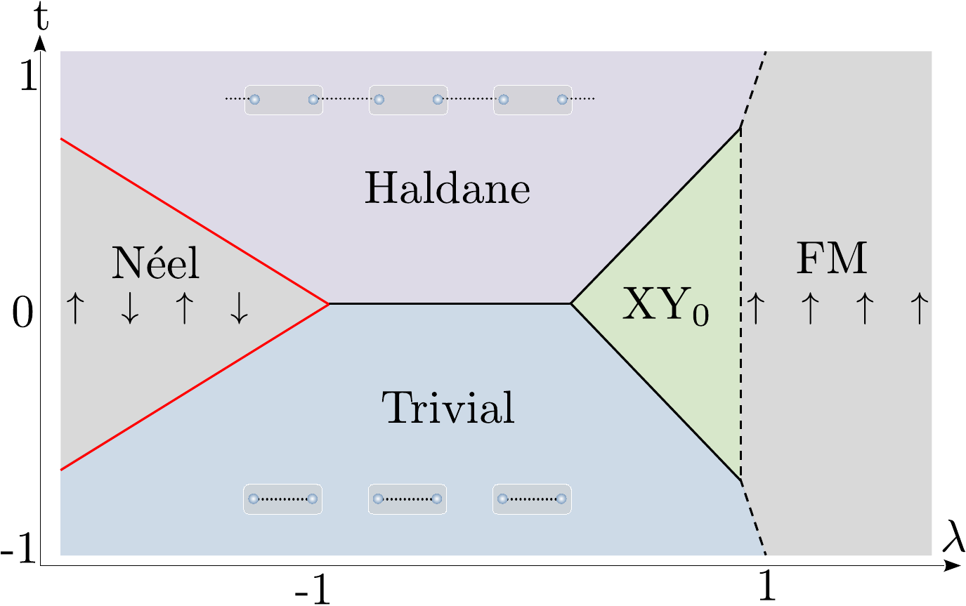
We study a one-dimensional chain of qubits (spin halves). There are two ways to view the system. The first, shown in the top panel of Fig. 1 is to regard the system as a single chain where the Hamiltonian can be written as an XXZ chain with alternating bond strength and next-nearest-neighbor coupling as follows (the coupling constants and are reversed in sign compared to the usual convention for convenience)
| (1) |
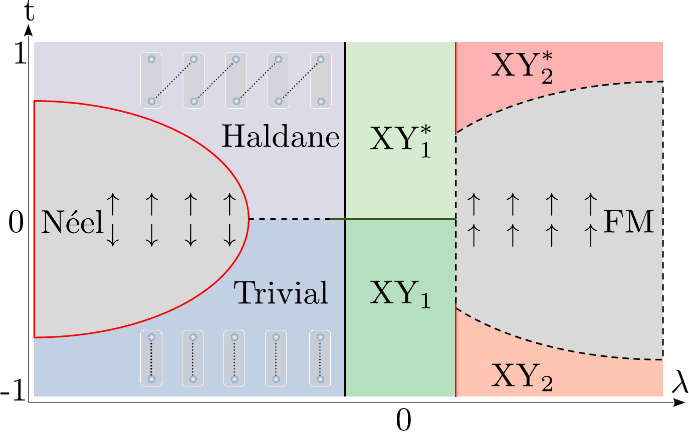
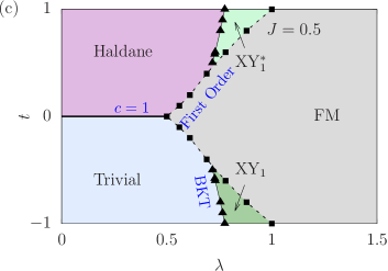
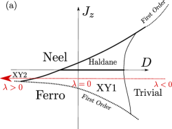
are spin operators, defined as usual in terms of Pauli matrices: . The model has four parameters: and . We will be interested in two-dimensional phase diagrams varying and with and fixed. The representation in Eq. 1 appropriate in the limit of small when the next-nearest neighbor (nnn) term can be regarded as a perturbation of the bond-dimerized XXZ spin chain. The phase diagram in this limit is well known [24, 23], and is schematically shown in Fig. 2. We are interested in the gapless Luttinger liquid phase labeled XY0 which can be adiabatically connected to the one found in the phase diagram of the XXZ model (i.e. for ).
 |
 |
For large , the Hamiltonian is appropriately visualized as a two-rung spin ladder as shown in the bottom panel of Fig. 1, with the following presentation:
| (2) | ||||
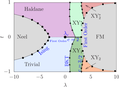
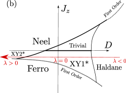
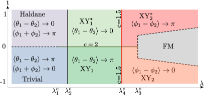
labels the rungs of the ladder and contains, respectively, the even and odd lattice spins of Eq. 1. represents the intra-rung and represent the inter-rung XXZ couplings. In this limit, it is appropriate to treat as perturbations to . The schematic phase diagram in this limit which we find is shown in Fig. 2. Our prime interest in this phase diagram are the four Luttinger liquid phases labelled XY1, XY, XY2 and XY. We will show that all five gapless phases found in the large and small phase diagrams are distinct from each other meaning they cannot be connected without encountering a phase transition. Furthermore, we will also show that one of these, XY is a topological Luttinger liquid containing stable edge modes [14, 19, 18]. A positive finite , introduces intra-chain ferromagnetic correlations, which is crucial to open up various gapless phases as will be discussed in detail.
Parts of the large- phase diagram have appeared in previous studies [25, 26, 27, 28, 29, 30, 31, 32]. However, the complete set of gapless phases, their symmetry distinction and topological properties have not been identified to the best of our knowledge. This will be the focus of our work. We will understand these (a) using bosonization in Sections III and IV, (b)numerically, using density matrix renormalization group (DMRG) in Section V and (c) by mapping Eq. 2 to effective spin-1 models in Section VI.
II.2 Symmetries
| Symmetry | Small | Large |
|---|---|---|
| spin rotations | ||
| spin reflection | ||
| lattice parity | ||
| lattice translation |
Global symmetries of the system will play an important role. Four symmetries are sufficient to characterize all phases and transitions: (i) on-site symmetry that corresponds to spin rotations, (ii) on-site spin reflections (iii) lattice symmetry that corresponds to a bond-centred reflection in the small- version and site-centred reflection followed by layer-exchange in the large- version, (iv) lattice translations. The symmetry action on spin operators is shown in Table 1. Altogether, the full symmetry group is 111The and symmetries do not commute and together form the non-abelian group . Additional symmetries are present in the model (eg: time-reversal) but are not needed for our purposes. In other words, they can be explicitly broken without changing the nature of the phase diagram.
II.3 Phases and transitions
The main focus of our work are the five symmetry enriched Luttinger liquid phases XY0, XY1,2 and XY shown in Fig. 2. At long distances, all five of these are described by a compact boson conformal field theory with central charge . However, the presence of global symmetries results in distinctions between them. The microscopic symmetries shown in Section II.2 are imprinted on the long-wavelength degrees of freedom in different ways in each of the five phases, and as a consequence, they cannot be connected without encountering a phase transition or an intermediate phase. Conversely, the distinction can be eliminated between the phases, and they can be connected by explicitly breaking appropriate symmetries. This will be explained in detail using bosonization analysis in Section III.
More operationally, we will show that the distinction between these phases can be demonstrated using appropriate local and string operators. While XY0, XY1 and XY can be distinguished by local operators only, XY2 is distinguished from XY using string operators. This is comparable to the situation with gapped phases, where symmetry protected topological (SPT) phases [34] are distinguished by string operators. The phase diagrams shown in Fig. 2 contain a non-trivial SPT phase, the Haldane phase, which is distinguished from the trivial paramagnet using an appropriate string operator. We will see that the same string operator can be used to distinguish between XY2 and XY. Furthermore, like the Haldane phase, the XY phase will also contain protected edge modes but with reduced degeneracy. This will also be explained in Section IV using bosonization and confirmed numerically in Section V.
We are also interested in the phase transitions between the gapless phases shown in Fig. 2. These are summarized below along with the universality class.
-
•
XY1 to XY: c = 2 theory of two compact bosons.
-
•
XY1 to XY2 and XY to XY: c= theory of a compact boson CFT combined with a Ising CFT.
The second order transitions out of the gapless phases to either the Haldane or trivial phase in Fig. 2 is of the BKT type, when the value of the Luttinger parameter is such that the perturbation that drives the gapped phase becomes relevant. We will also understand these using bosonization in Appendix B and confirm them numerically in Section V.
Finally, the gapped phases present in Fig. 2 (Haldane SPT, trivial paramagnet and symmetry breaking Néel and ferromagnet) as well as transitions between them are well understood. We mention them for completeness– The Haldane and trivial phases are separated by a compact boson CFT for small and by a first-order transition for large . The Néel phase is separated from the trivial and Haldane phases by an Ising CFT and its symmetry-enriched variant, respectively [18] for both small and large . Finally, the FM is separated from the Haldane and Trivial phases through a first-order transition for small .
III Bosonization analysis I: characterizing the gapless phases
In this section, we will study the properties of various gapless phases and transitions between them using abelian bosonization. We begin by reviewing the framework applicable to the parameter regimes for small and large and then proceed to understand the various gapless phases in two ways: (i) by using the effective action of microscopic symmetries on the CFT and (ii) the behavior of local and non-local operators carrying appropriate symmetry charges. We delay a thorough analysis of the topological aspects of the XY phase to Section IV.
III.1 Bosonization formulas for small and large and conventional description of phases
For small , the Hamiltonian shown in Eq. 1, can be treated as a single XXZ spin chain with perturbations. In the regime of our interest, it can be bosonized using standard arguments [20, 35] as follows (see Appendix A for more details)
| (3) |
and are canonically conjugate compact boson fields with unit radii satisfying the algebra [21]
| (4) |
and etc are bosonization prefactors whose precise values are not important. The Luttinger parameter and the velocity are related to the Hamiltonian parameters [36] (see Appendix A). The bosonized forms of the spin operators are
| (5) |
Equation 3 is a compact boson conformal field theory (CFT) with central charge perturbed by vertex operators with scaling dimensions [37, 21]
| (6) |
Note that we have only shown the most relevant operators, with the smallest scaling dimensions in Eq. 3. The ellipses represent other operators that are not important for our purposes. The the small- phase diagram shown in Fig. 2 can be qualitatively reproduced from Eq. 5 by tracking the relevance 222Recall that a scaling operator is relevant in d+1 dimensions if its scaling dimensions satisfies . of (see Appendix B for a detailed discussion). Bond dimerization introduces the vertex operator and the interaction while introduces . For now, we note that in the regime when , all perturbations are irrelevant and correspond to the XY0 gapless phase.
A different starting point is useful in the large limit. We now interpret the Hamiltonian in Eq. 2 as two XXZ spin chains with intra- and inter-rung perturbations. Each leg can be bosonized appropriately to obtain the following two-component compact-boson theory [35]
| (7) |
where and are compact boson fields satisfying
| (8) |
and are again unimportant bosonization prefactors and we have only shown the most important operators. The bosonized forms of the spin operators are
| (9) |
The above theory represents a CFT with perturbations. We have only retained primary [21, 37] scaling operators in Eq. 9. This is sufficient to determine the structure of the phases and transitions, which is our focus. However, it is known [39] that descendant operators must be considered to understand certain incommensurability aspects of correlations. The large- phase diagram can be qualitatively reproduced using Eq. 9 by carefully tracking the relevance of the operators , and (details of this can be found in Appendix B). Here, we again focus only on how the four gapless phases can emerge. An important fact is that the scaling dimensions of the various operators listed above are not all independent. In particular, we have . Therefore, it is impossible for both and to be irrelevant at the same time, and for any , the theory is unstable and flows to a Luttinger liquid phase with or a gapped phase [26, 27, 35] as seen in Fig. 2. The first, which is of our main interest, occurs when all other operators, especially are irrelevant. The nature of the resulting gapless phase depends on: (i) which among and has the smaller scaling dimensions at . This dominates long-distance physics for resulting in the pinning of either or and (ii) the value to which or is pinned, depending on the sign of and . The four possibilities result in the four gapless phases shown in the large- phase diagram of Fig. 2 as follows.
-
1.
XY1: ,
-
2.
XY: ,
-
3.
XY2: ,
-
4.
XY: , .
There are two critical scenarios which we now discuss: when , the theory flows to a theory corresponding to a compact boson with Ising CFT [40]. For corresponds to a phase transition described by the parent two-component compact boson theory when the pinned value of the appropriate fields changes. At this stage, let us point out elements of the discussion above that already exist in the literature. The competition between and leading to different phases was discussed in refs. [40, 27, 35]. The importance of the precise values to which the fields are pinned was appreciated relatively recently [14, 19, 18] where it was shown that produces a gapless phase with edge modes.
However, we must be careful in using these pieces of information to conclude that we have distinct phases of matter. It was recently pointed out that this kind of distinction can disappear suddenly [22, 23, 41]. A more robust characterization arises out of symmetry considerations which we now turn to. We do this in two complementary ways. First, we establish the fate of the microscopic symmetries shown in Tables 1 and 2 in the deep IR for each of the gapless phases. The effective theory for all of them is that of a single compact boson. We show that in each of the five phases, the microscopic symmetries act in inequivalent ways that cannot be deformed into each other. Second, we study how appropriately charged local and nonlocal operators behave in the different phases and show a complete list of operators with distinct charges that can serve as order parameters to distinguish the different gapless phases. Our work therefore characterizes a rather subtle interplay of symmetries and topology leading to the emergence of novel gapless phases.
III.2 Multiversality along the surface
An interesting feature of the phase diagrams shown in Fig. 2 is the nature of transition separating the Haldane and Trivial phases along parts of the surface. In the small- limit, we see from Eq. 3 that the critical theory corresponds to a compact boson CFT with central charge . In the large- diagram, the situation is different. Consider the effective theory in Eq. 7 and set . This is a CFT with perturbations and describes various transitions and phases along the surface. In particular, the transition between XY1 and XY corresponds to the theory when all perturbations are irrelevant or tuned away. As we move along this surface, the operator becomes relevant and gives us a gapped theory with two ground states which precisely correspond to those of the Haldane and trivial phases and therefore represent a first-order transition between them (see Appendix B for a detailed discussion). Now consider the transition between XY1 and the trivial phase. This is driven by the operator becoming relevant. Since has a smaller scaling dimension than , the XX1 -to- trivial critical line strikes the line well before the first-order transition sets in. The same is true for the XY -to- Haldane transition. Consequently, we expect that a segment of the transition (close to the gapless phases) between the Haldane and the trivial phase will also be described by the CFT before becoming first-order as shown in Fig. 2. This situation is unusual because it is a different universality class (with a different central charge) compared to the small- transition between the same phases. Furthermore, in both cases, the transitions are reached by tuning only a single parameter, without additional fine-tuning.
The presence of multiple stable universality classes that separate the same two phases has been termed ‘multiversality’ [22, 23]. Although there are no physical reasons forbidding multiversality, models that exhibit it are surprisingly rare. We see that the spin ladder model considered in this work exhibits the phenomenon under relatively generic conditions and symmetries (compare this to the example in Ref.[23] where multiversality was observed under more restrictive symmetries and destroyed when symmetries were reduced).
III.3 Distinguishing gapless phases through effective symmetries
| Small | Large | |
|---|---|---|
We begin this subsection by listing the action of symmetries listed in Table 1 on the compact boson fields in both the small and large versions [42, 35]. This is shown in Table 2 and is obtained by comparing the action on the lattice operators shown in Table 1 with the dictionary shown in Eqs. 5 and 9 (see Appendix A for more details). We want to understand the fate of these symmetries in various gapless phases. The long wavelength physics of each of these gapless phases is identical and corresponds to that of a single compact boson with a Hamiltonian of the form
| (10) |
How do the microscopic symmetries act on the long wavelength effective fields? Observe that the compact boson theory itself has various symmetries such as
| (11) |
which form the group 333The two symmetries also contains a well known mixed anomaly [89]. The full collection of symmetries of the compact boson CFT is larger and contains the group of conformal transformations as well as other generators that may not even form a group structure [90, 91]. For our purposes, the ones listed in Eq. 11 that form are sufficient..
The action of symmetries can also be studied in the spectrum of local scaling operators with scaling dimensions where and are integers. These read as follows
| (12) |
The question we are interested in is how the microscopic symmetries of spins listed in Table 1 attach themselves to those of compact boson degrees of freedom, . In other words, we we are interested in the homomorphisms . Distinct homomorphisms will lead to inequivalent symmetry enriched Luttinger liquids that cannot be adiabatically connected. We will determine this for each phase one-by-one to confirm this.
III.3.1 Effective symmetries of XY0
Let us begin with the gapless phase seen in the small- limit, XY0. The effective action of symmetries were already obtained using the bosonization formulas as listed in Table 2. This can also be used to determine the action on various scaling operators as shown in Table 3. We see that the microscopic attaches itself to , to a simultaneous action of and , and to a composite action of simultaneous rotation of and action while UV lattice translations have no effect in the IR.
III.3.2 Effective symmetries of XY1 and XY
| XY1 | |||
| XY | |||
We now consider the gapless phases in the large- limit obtained when dominates at long distances pinning . To determine the nature of the resulting compact boson CFT the system flows to, we perform the following transformation which preserves the unit compactification radius of the fields as well as the canonical commutation relation Eq. 8
| (13) |
When is pinned, its conjugate is disordered and we obtain physics at long distances by setting
| (14) |
The effective theory is simply that of the unpinned canonically conjugate pair of fields, = and with a Hamiltonian of the form shown in Eq. 10.
Using Eq. 14 and the action of the symmetries on the compact bosons obtained from bosonization at large shown in Table 2, we can read off the effective symmetry action on the and as well as on the spectrum of scaling operators as shown in Table 4. First, compare these with Table 3. We see that the actions of and are identical in all three phases. However, the action of distinguishes XY0 from the other two. Finally, the symmetry action of depends on the value of and distinguishes between XY1 () and XY (). Observe that both electric scaling operators (i.e., those carrying charge) with the smallest scaling dimensions, and are pseudo-scalars for XY1 and scalars in XY respectively. Thus, we have succeeded in establishing that XY0, XY1 and XY are distinct from each other.
III.3.3 Effective symmetries of XY2 and XY
| XY2 | |||
| XY | |||
Finally, we turn to the large- gapless phases obtained when dominates at long distances and pins . To get the effective symmetries of the resulting compact boson CFT the system flows to, we perform a different transformation from Eq. 13
| (15) |
When is pinned, its conjugate is disordered and we obtain the long distance physics by setting
| (16) |
The effective theory is simply that of the unpinned fields and with an effective Hamiltonian of the form shown in Eq. 10.
Using Eq. 16 the symmetry action on the effective low-energy fields and on the spectrum of operators can be read off from Table 2 and is summarized in Table 5. The most striking feature is that the field is a charge 2 operator for the symmetry. Consequently, the smallest charge carried by the spectrum of scaling operators is . This immediately shows that XY2 and XY are distinct from XY0, XY1 and XY. Let us now focus on the effective action of which seemingly depends on the value of and distinguishes XY2 from XY. This is not true– the symmetry actions are merely related by a change of basis. However, keeping track of other symmetry charges exposes the distinction. Consider magnetic scaling operators (those without any charge) with the smallest scaling dimensions, and . We see that in XY2, the operator with charge () transforms as a scalar under whereas the operator without charge () transforms as a pseudoscalar. This situation is precisely reversed for XY where the charged operator is a pseudoscalar, whereas the neutral operator is a scalar. This completes the proof that the five gapless phases are distinct.
III.3.4 Explicit symmetry breaking
Observe that all four microscopic symmetries were important in establishing these distinctions. Explicitly breaking certain symmetries eliminates the distinction between certain phases and opens a potential path to connect them without phase transitions or intermediate phases. Let us look at a few instances.
-
1.
If we break , the distinction between XY2 and XY is eliminated and reduces five phases to four: XY0, XY1, XY and (XY XY).
-
2.
If we break , the distinction between and XY is eliminated, as well as between and XY and reduces the five phases to three: XY0, ( XY XY) and (XY XY).
-
3.
If we only preserve and break all other symmetries, the five phases reduce to two: (XY XY XY) and (XY XY).
III.4 Local and non-local observables
| XY0 | XY1 | XY | XY2 | XY | |
| alg | exp | alg | exp | exp | |
| alg | alg | exp | exp | exp | |
| 0 | 0 | 0 | 0 | 0 |
We now turn to how we can physically characterize various gapless phases using local and non-local observables. We will use the previously determined effective symmetry action listed in Tables 3, 4 and 5 to guide us in this. We will focus on two local operators and a non-local string operator defined as follows (in both the small () and large () representations)
| (17) | ||||
| (18) | ||||
| (19) |
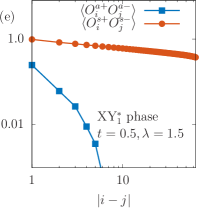
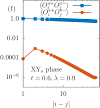
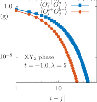
The nature of two-point correlation functions of the local operators and the expectation value of the string operator are summarized in Table 6 and completely characterize the phases. We see in Table 6 that local operators uniquely identify the XY0, XY1 and XY2 phases but cannot distinguish between the XY2 and XY phases, which the nonlocal operator can. In this section, we will see how this behavior can be determined using the bosonization formulas as well as using the effective symmetry action shown in Tables 3, 4 and 5. These predictions will also be confirmed numerically in Section V.
III.4.1 Local operator behavior from bosonization
Let us begin with XY0 where, using Eq. 5 the local operators can be bosonized as
| (20) |
In Eq. 20, we have suppressed the bosonization prefactors and retained only the most relevant scaling operators the lattice operators have an overlap with. Clearly, the two point functions of and are expected to have algebraic decay governed by the parameters of the effective compact-boson CFT that describe the phase at long distances. Recall that for a CFT, the correlation functions of the scaling operators with scaling dimensions scale as
| (21) |
Thus, at long distances , we expect
| (22) |
Let us now consider the large- phases where, using Eq. 9, we get
| (23) |
We have again suppressed bosonization prefactors and retained only the most relevant scaling operators. When we have the full theory along the line shown in Fig. 15 we see that both local operators have algebraic correlations. However, for , when or are relevant resulting in the different gapless phases, this changes. Consider the case where is the most relevant operator and pins . We can use the transformation shown in Eq. 13 and Eq. 14 to obtain the following.
| (24) |
We see that for each case , only one of the two operators / has vanishing overlap with scaling operators and has algebraic correlations whereas the other has exponential correlations:
| (25) |
is the effective Luttinger parameter shown in Eq. 10 that characterizes the effective compact boson CFT at long distances. We may wonder if the calculations above are modified if we include the corrections to the bosonization formulas represented by ellipses in Eq. 9. It turns out that the answer is no and can be verified by including all higher terms explicitly. A more powerful way is using symmetries, as will be discussed in the next subsection.
We now turn to the phases obtained when is dominant and pins . Using the transformation shown in Eq. 15 as well as Eq. 16, we get
| (26) |
We see that both and have no overlap with any scaling functions and therefore their correlation functions decay exponentially
| (27) |
We can check that this behaviour does not change even when corrections represented by ellipses in Eq. 9 are included. This can also be justified using symmetry arguments as we will now see.
III.4.2 Local operator behaviour from effective symmetry action
The correlations of local operators shown in Table 6 can also be understood directly by using symmetries. Let us begin by noting down the transformations of the local operators under the , and symmetries. This is shown in Table 7. At this point, let us remark that all local operators are charged under various internal symmetries. The non-local operator, on the other hand, although is neutral overall, has end points that carry charge. This is important to establish the topological nature of phases and will be discussed in Section IV. Now, we can ask if the transformations shown in Table 7 can be obtained in each of the five gapless phases using combinations of the scaling operators whose transformations are shown in Tables 3, 4 and 5. If the answer is yes, it will mean that the local operator will have algebraic correlations at long distances with the exponent determined by the scaling dimensions of the said operators with smallest scaling dimensions. If not, then the operators will have exponentially decaying correlations
XY0: Comparing the transformations shown in Table 7 and Table 3 tells us that and can have overlap with . Comparing the action tells us that the smallest operators that transform correctly are
| (28) | ||||
| (29) |
which is precisely what was obtained from the bosonization formulas in Eq. 20 and Eq. 22. This combination also transforms correctly under .
XY1 and XY: Comparing the transformations shown in Table 7 and Table 4 again tells us that and can overlap with . It is easy to check that no combination of scaling operators can simultaneously reproduce the and transformations of (for that is, XY1) and (for that is, XY) and therefore have correlations that decay exponentially. On the other hand, has the right transformation properties as (for i.e. XY1) and (for i.e. XY). This reproduces Eqs. 24 and 25.
XY2 and XY: The effective transformations in Table 5 tell us that all scaling operators have a minimum charge of and therefore there are no combinations of scaling operators that have the transformation properties of and and that have a unit charge as seen in Table 7. Consequently, the correlations of and have exponential decay in both XY2 and XY phases 444Note that lattice operators with charge 2 such as will have algebraic correlations in XY2 and XY phases as shown in [40].. This reproduces Eqs. 26 and 27.
III.4.3 Behaviour of the non-local operator
We now turn to the nonlocal string operator defined in Eq. 19 which can be bosonized in both the small- () and large- () limits as follows (see Appendix C for details)
| (30) | |||
| (31) |
where we have only shown operators with the smallest scaling dimensions and are non-zero coefficients whose values we do not fix. It is now easy to verify how behaves at large . From Eq. 30, we have
| (32) |
Therefore, when , we have . Among the phases without spontaneous symmetry breaking, this happens when for small and for large . From Figs. 14 and 15, we see that in the Haldane and XY phases whereas in the trivial gapped phase and other gapless phases XY0, XY1 and XY, for sufficiently large . This confirms the remaining entries of Table 6.
IV Bosonization analysis II: the topological nature of XY
We now focus on the XY gapless phase and study its topological nature. First, we show that it has protected edge modes and then discuss the nature of the topological phase. In particular, we show that the gapless topological phase is not ‘intrinsically gapless’ and briefly discuss a related model where it is.
IV.1 Edge modes
A hallmark of gapped symmetry protected topological phases such as topological insulators and superconductors is the presence of protected edge modes degenerate with the ground state, which have exponentially small splitting at finite system sizes. Gapless topological phases are defined as those that have edge modes protected by symmetries and can be sharply identified at finite volumes by exponential or algebraic splitting with coefficients different from bulk states [14, 19, DHLee_Gapless_jiang2017symmetry, 15, 16] . Recall that XY was characterized by a nonzero expectation value of the string operator whose endpoints were charged under . The following argument presented in [19, 18] shows that this automatically implies the presence of edge modes. Let us first present the argument using lattice operators and then using bosonization.
IV.1.1 Argument using lattice operators
Let be the ground state of the XY Luttinger liquid which has string order
| (33) |
We also know that is invariant under the symmetries shown in Table 1. Let us consider rotation by angle generated by the following operator (we only consider the large notation for convenience).
| (34) |
This operator acts on a finite chain of length with unit cells labeled . Let us now consider the action of the string operator defined on the full length of the chain, i.e.
| (35) |
We use this along with to get the following result.
| (36) |
By cluster decomposition, we have
| (37) |
This proves that when we have string order, we also have edge magnetization. Since and are charged under symmetry , we can interpret this result as spontaneously breaking the symmetry at the edges and resulting in degenerate edge modes.
IV.1.2 Argument using bosonization
It is nice to obtain the same result using bosonization. Let us first write down the bosonized version of (see Appendix C)
| (38) | ||||
| (39) |
In the phases with , letting the string operator span the length of the system setting we have
| (40) |
By cluster-decomposition, we get
| (41) |
Using Eqs. 31 and 39, this reduces to
are some constants whose precise values are irrelevant. We see that are proper local operators (without fractional coefficients) carrying charge. Therefore, we have spontaneous symmetry breaking at the edges and associated boundary degeneracy whenever we have and unbroken symmetry, such as the Haldane and XY phases.
IV.2 Why XY is not an intrinsically gapless topological phase?
In the taxonomy of gapless topological phases [14, 19, 17, 15, 16], a special role is played by so-called intrinsically gapless topological phases [19, 45, 46]. These are gapless phases with stable edge modes protected by symmetries that do not allow gapped topological phases. In this sense, the topological nature is intrinsically gapless. Phase diagrams in which intrinsically gapless topological phases can be found cannot, by definition, contain gapped topological phases. Therefore, the phase diagrams shown in Fig. 2 that contain the Haldane phase, which is a gapped topological phase, make it clear that the XY phase is not intrinsically gapless. This is because the symmetries of the model protect both gapless and gapped topological phases. We can ask whether we can break certain symmetries to preserve only the gapless topological phase but eliminate the gapped one. We now show using bosonization that this too is not possible.
Let us focus on the large limit where XY is present. From Fig. 15, we see that the gapped Haldane phase is obtained when whereas the XY obtains when . Let us consider the possibility of eliminating the Haldane phase that has a gap while preserving XY by adding an operator that ensures that can be tuned smoothly to zero, while can only be pinned to or . The operator that achieves this is
| (42) |
However, note that the addition of Eq. 42 simultaneously breaks both and symmetries. Therefore, any lattice operator that produces Eq. 42 also generically produces an operator of the form
| (43) |
which smoothly tunes the pinned value of to zero and therefore eliminates XY 555Note that Eq. 43 that breaks but preserves can be introduced to eliminate XY but preserve the Haldane phase. But this is not interesting..
IV.3 A related model where XY is an intrinisically gapless topological phase
We now present a model where XY is an intrinsically gapless topological phase. We work in the large- limit and modify the Hamiltonian in Eq. 2 as follows
| (44) | ||||
The presence of the new term, preserves all original symmetries shown in Table 1 but importantly introduces a new on-site symmetry which exchanges the two legs. The action on spin operators and large- bosonized variables is as follows.
| (45) |
Remarkably, the bosonized version of Eq. 44 is identical to Eq. 9 and therefore should contain the same phases although in different parameter regimes. Let us now consider including lattice operators that explicitly break the and symmetries but preserve the new symmetry shown in Eq. 45. In the continuum limit, this introduces only the perturbation shown in Eq. 42 but not Eq. 43 since the latter breaks . As explained above, this eliminates the Haldane phase. The equivalent of XY phase in this model is an intrinsically gapless topological phase. Indeed, the residual on-site unitary symmetry is known to not host any gapped symmetry protected topological phases in one dimension [48]. We leave the numerical study of the model in Eq. 44 to future work.
V Numerical Analysis
In this section, we numerically analyze the system at hand and validate the analytical results predicted above. We map the spin system to hard-core bosons, where the on-site occupancy is restricted to . The Hamiltonian in terms of hard core bosons (see Eq. 2) becomes
| (46) |
where () annihilation (creation) operators and with being the number operator for site . The ground state of the model Hamiltonian is computed using the Density Matrix Renormalization Group (DMRG) method [49, 50, 51]. The bond dimension is taken to be , which is sufficient for convergence for typical system sizes where is the total number of sites in the system. Unless otherwise stated, sites are labeled using a single-site label convention of Eq. 1.
V.1 Diagnostics, Phases and Phase transitions
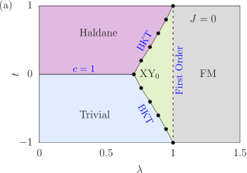
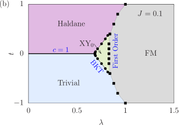
We explore the parameter space in the plane with fixed and identify the phases and their transitions. The most illustrative limit is to first investigate when [52] where the system, in the absence of any dimerization (), undergoes a first order phase transition at (see Fig. 4(a)). engineers gapped phases between , however is trivial and is topological (Haldane phase) in nature. A gapless phase (XY0) opens between where both perturbations and are irrelevant. Introducing a small finite , not unexpectedly, only renormalizes the phase boundaries (see phase diagram in Fig. 4(b)) reducing the size of the gapless XY0 phase. A further increase in leads to the emergence of two new gapless phases (XY1) and XY as XY0 disappears (see Fig. 4(c)) and we get the large picture.
To explore the large phase diagram schematically shown in Fig. 2, a particularly illustrative parameter choice is to explore the phase diagram for fixed as shown in Fig. 5 (). Four distinct symmetry enriched critical phases are clearly obtained. To conclusively characterize the phase boundaries and the nature of their transitions, we use a host of diagnostics which we now discuss.
V.1.1 BKT Transitions
Transitions from the trivial gapped phase to XY1 and the Haldane phase to XY belong to the BKT universality class. To characterize these transitions, it is useful to note that in the (hard-core) bosonic language, the XY1 and XY phases are -superfluids (SF()) phases [53, 54]. In such systems, the momentum distribution is given by
| (47) |
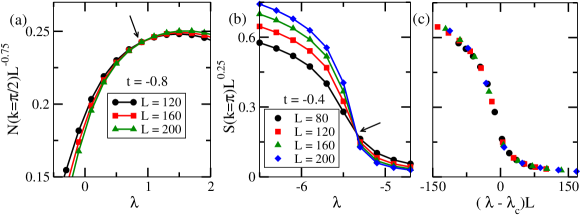
(where ) and is expected to show a sharp peak at . At the transition itself, the finite-size scaling of carries the signature of an underlying BKT transition. For example, at the critical point, the BKT ansatz predicts which can be used to extract the value of [55, 56]. The perfect crossing of the data for different lengths at as shown in Fig. 6(a) indicates a BKT transition which has the Luttinger parameter of value as expected from Section III (see also Appendix A). This is found to be true for all values of using which the phase boundaries to the SF() (XY1) phase of Fig. 5 have been obtained.
V.1.2 Ising transitions
The transitions from the Néel to trivial and Haldane (circles), from XY1 to XY2, and from XY to XY phase are found to be of Ising type (see Fig. 5). Such Ising transitions can be characterized by analysing the finite size scaling of the structure factor defined by
| (48) |
In the Néel state, shows a peak at signalling antiferromagnetic correlations. At the Ising transitions, it is known that follows a scaling ansatz such that at the critical point is invariant for different with exponents and [57, 58]. The perfect crossing of as shown in Fig. 6(b), and eventual collapse of all the data points, shown in Fig. 6(c), for different in vs. plane near the transition point implies an Ising phase transition at with a critical point . We use the same approach to calculate the Ising phase boundaries in the phase diagram (Fig. 5).
V.1.3 transition between gapless phases
Unlike the previous Ising transitions where one transits from a gapless to a gapped phase, the Ising transitions that appear between XY1 to XY2 and XY to XY are gapless-to-gapless transitions. Since this CFT appears in addition to the existing compact boson, the total central charge of the transition is expected to be . Phase transition points are quantified by analyzing fidelity susceptibility () where
| (49) |
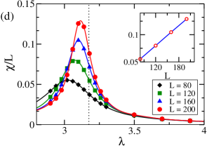
where is the ground state at . At the phase transition point, develops a peak, and the height of the peak diverges linearly with for the Ising transition [59, 60, 61]. In Fig. 6(d), we plot for different system sizes, which shows an increase in the peak height with . The inset of Fig. 6(d) shows the linear divergence of the peak height, implying the Ising transition. The critical point of the transition is determined by extrapolating the position of the peak to the thermodynamic limit, which is marked by the dashed line in Fig. 6(d).
V.1.4 Multiversality along the line
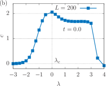
On line, the gapless phase with starts at which is a BKT transition point that can be calculated using finite size scaling of single particle excitation gap [57]. The excitation gap at half-filling can be defined as,
| (50) |
where and is the number of particles in an excitation. The invariance of with at the critical point and the collapse of all the data in vs. plane, where
| (51) |
at and near the critical point with a suitable choice of constants and predicts the BKT transition point (see Fig. 8).
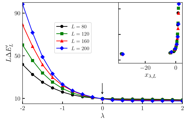
From Fig. 5, we see that the line separates the gapless phases XY1 and XY as well as the trivial and Haldane gapped phases. The latter phases are separated by a different universality class with for small . This is a numerical confirmation of the ‘multiversality’ [23, 22] phenomenon discussed in Sections III and A.
V.1.5 First order transitions
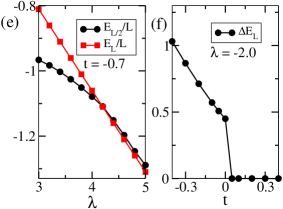
Finally, the transition between the trivial and the Haldane gapped phase for negative values of at large , or that between any of the phases to FM is first-order in nature. These can be characterized by analyzing the level crossings between eigenstate energies. For instance, in the case of transitions to the FM phase, we plot the ground state energy at boson half-filling (), which corresponds to zero magnetization sector, and completely filled (), which is equivalent to fully magnetized case (FM phase) across the boundary in Fig. 6(e). The crossing between and determines the first-order transition points, which are marked by squares in the phase diagram (Fig. 5). On the other hand, the sharp jump in single particle excitation gap (Eq. 50 with ) at for the transition between the trivial gapped to Haldane gapped phase, as shown in Fig. 6(f), signifies a first-order transition (also see Fig. 5).
V.1.6 Central charge
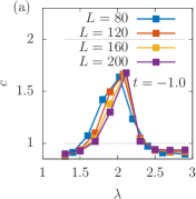
Now we want to give numerical evidence for the central charge predicted by the bosonization analysis. We find the central charge () by fitting the bipartite Von-Neumann entanglement entropy () to its conformal expression [62]
| (52) |
Figure 7(a) show how changes at the transition between XY1 and XY2 phases according to Fig. 5. In Fig. 7(b), we represent along the line that cuts through the interface between the XY1 and XY2 phases. As discussed above in the analytical analysis, we find from the numerical analysis, although not exactly, that the is close to in the XY1 XY transition and at the Ising transition point between the phases XY1 and XY2, the is close to (upto finite size effects).
V.2 Characterising gapless phases
Since the gapped phases and particularly ordered phases are well understood and can be easily characterized by conventional order parameters, here we will focus our discussion on the gapless phases and their characterization.
V.2.1 String Order Parameter
A particularly useful tool, which also helps in distillation of the topological features of the gapless phases, is the string order parameter (see equivalently Eq. 19 upto a phase) where
| (53) |
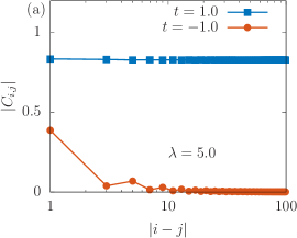
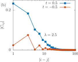
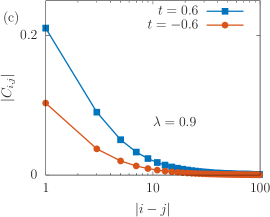
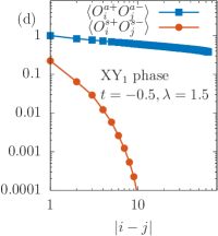
and . The string order parameter , not unexpectedly, shows a finite value in the Haldane (gapped) phases in the system (not shown) [63, 58]. Interestingly, the same order parameter also takes nontrivial values in XY, proving that it is a gapless topological phase. In Fig. 9(a) the behavior of is shown for both XY2 (circles) and XY (squares) - one finds that, unlike XY2, in XY, takes a finite value that does not decay with . Similarly in Fig. 9(b) we plot within the phase XY1 (circles) and XY (squares), and in Fig. 9(c), we plot it in the XY0 phase. In both plots, the string-order parameter vanishes, showing that these phases are trivial in nature.
V.2.2 Local Order Parameters
The nature of long-range correlations can also distinguish between the different phases, as shown in Table 6. To this end, we calculate and where and to distinguish between the trivial, XY1, XY and XY0 phases. The results are shown in Fig. 9(d-g) for all the gapless phases. We see a contrast in the nature of these correlations in two phases. The () falls exponentially (algebraically) with distance in the XY1 phase. Whereas, in the XY phase, the behavior flips. However, in XY0 and XY2, both correlation functions are algebraic or exponential, as shown in Figs. 9(f) and (g), respectively.
V.2.3 Edge states
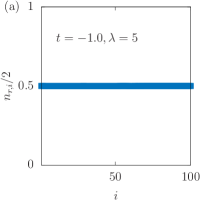
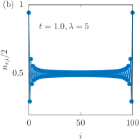
The topological XY phase exhibits edge states, a hallmark property of such topological phases. In Fig. 10(a) and Fig. 10(b), we plot the number of particles in strong rungs, where the hopping and interaction coupling are large (even or odd rungs) according to the construction of the system, for the phases XY2 and XY, respectively. For XY, two edge sites do not belong to the strong bond where we plot . We can see that, only for the XY phase (Fig. 10(b)), the system exhibits exponentially localized occupied edge states.
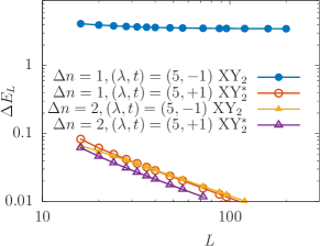
The edge states manifest gapless excitations at the edges of the system. To confirm this property, we plot the energy gap for the excitation (Eq. 50) at half-filling. In Fig. 11 we plot for (circles) and (triangles) in the phases XY2 (solid symbols) and XY (empty symbols). In both phases, the elementary excitation in bulk is (a pair of particles on the strong rungs), which is gapless. This can be confirmed from the algebraic decay of . In the XY phase, due to the presence of edge states, which can be occupied by a single particle, we see algebraic decay of even with . In the XY2 phase, however, single particle excitation is gapped where saturates to a finite value.
VI Mapping to effective spin–1 models
The connection between phase diagrams of spin ladders and higher-spin chains is rather well known [40]. Certain parts of the phase diagram shown in Fig. 2 too can be determined using a mapping to an effective spin 1 model. This provides both consistency checks and physical insights into the phases. To do this, let us begin with the Hamiltonian in Eq. 2 and perform a change of basis
| (54) |
which results in the following change in and
| (55) |
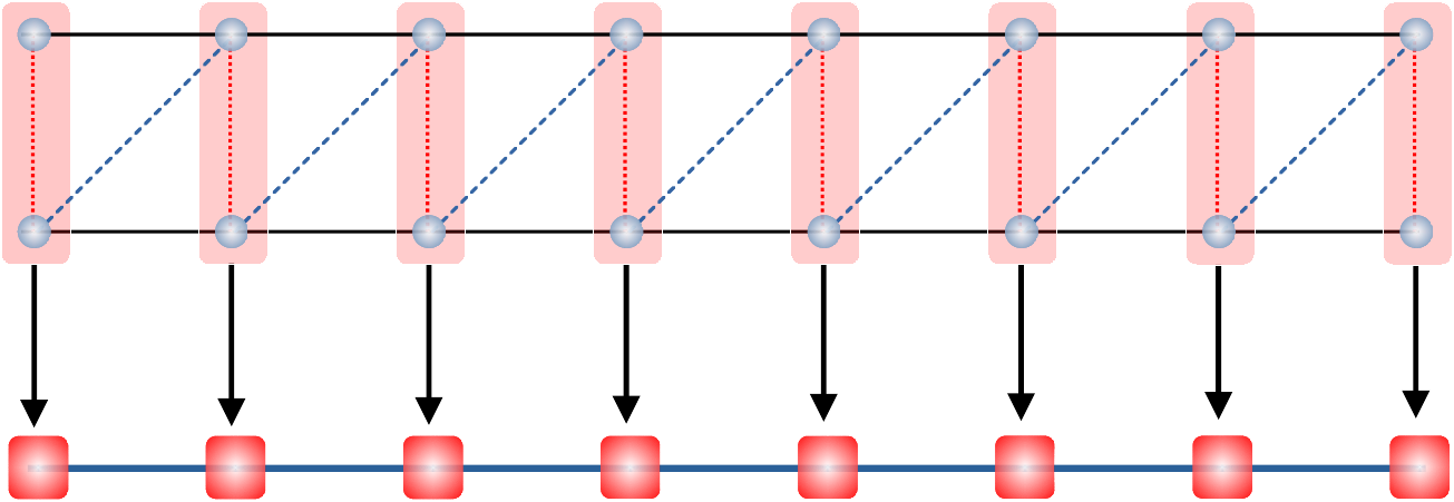
Let us first consider the parameter regime when is dominant, i.e. . Since decouples into disjoint pieces each of which has support on two spins living on vertical bonds as shown in Fig. 12 and takes the form
| (56) |
it can be easily diagonalized as follows (suppressing site labels for clarity)
| (57) |
and represent eigenstates of with eigenvalues respectively. We see that for all values of , have the lowest energies. We can project the two-spin Hilbert space on the vertical bonds of every site onto this three-dimensional subspace using the following projection operator
| (58) |
as schematically shown in the top figure of Fig. 12 to get an effective spin-1 chain with Hamiltonian
| (59) |
where
| (60) |
are the spin 1 representations of the angular momentum algebra with representations
| (61) |
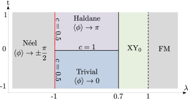
The Hamiltonian in Eq. 59 is the familiar spin-1 XXZ model with uniaxial single-ion-type anisotropy whose phase diagram is known [64] and is schematically reproduced in Fig. 13. For the parameter regime close to , the phases and transitions of the Hamiltonian in Eq. 2 are qualitatively reproduced by that of Eq. 59. For example, consider the limit when Eq. 59 reduces to
| (62) |
If is fixed to a small value, as is tuned, we see from Fig. 13 that Eq. 62 passes through the large-D (trivial), XY1, XY2 and the Ferromagnetic phases– the same as what is seen in Fig. 2. It is worth emphasizing the crucial role of which builds residual ferromagnetic correlations between effective spin-1s, thus leading to the realization of interesting gapless phases. Through the spin-1 mapping we are able to see that in order to access the XY2 phase, we need to fix to be small as was done in our numerical investigations.
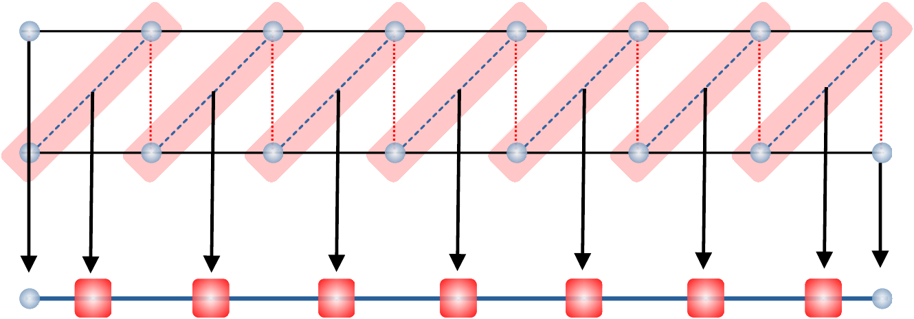
Let us now consider the limit when the Hamiltonian Eq. 2 is dominated by . First, let us observe that with periodic boundary conditions, is induced by a unitary transformation generated by a single-site translation on one of the legs of the ladder . As a result, the phase diagram for Eq. 2 is perfectly symmetric under . The identity of the phases, however, can change under this map. In particular, the unitary transformation is ill defined with open boundary conditions and therefore it is conceivable that the distinction between the regions related by , is topological in nature. We will now map the dominant Hamiltonian to a spin 1 chain. To do this, we repeat the steps above and observe that with periodic boundary conditions, decouples into disjoint pieces, each of which has support on two spins, this time living on the diagonal bonds as schematically shown in the bottom figure of Fig. 12. We again perform a convenient change of basis similar to Eq. 55 to get the following local term
| (63) |
This is easily diagonalized as
| (64) |
where and are as defined as in Eq. 57. Projecting onto the low-energy Hilbert space spanned by on each diagonal bond, we again get an effective spin-1 chain with the following Hamiltonian
| (65) |
with
| (66) |
We have denoted the bond between spins and by . So far, Eq. 65 looks identical to Eq. 59 with the replacement . However, a change occurs with open boundary conditions. There is no natural association of the boundary qubits with any diagonal bond. As a result, it survives the the projection and remains as a qubit on the ends of the chain. The effective Hamiltonian with open boundary conditions is thus
| (67) |
where and are the same as in Eq. 66. is the effective boundary Hamiltonian,
| (68) |
where the coupling constants to the boundary qubits and are
| (69) |
The picture above suggests an interesting alternative method of analysis to the abelian bosonization of Section III by treating the boundary spin 1/2 as a quantum impurity [65], however, we will not pursue this route in this work and leave it for future work.
Let us make a few comments on the limitations and utility of the mapping to a spin 1 chain before we proceed to a discussion of the phases in the effective Hamiltonian for the limit. Recall that for the limit, the phase diagram for the spin 1 XXZ chain accurately reproduces the phases of the spin ladder. To identify the phases of the spin 1 XXZ with that of Eq. 2 in the limit, we need additional tools, although plausible arguments can be made, especially for the gapped phases. For instance, it is clear that the identity of the Ferromagnet obtained for large remains the same in Eqs. 67 and 59 as can be easily seen by taking to a large value in Eq. 2. The identities of the large-D and Haldane phase in Eq. 59 are reversed in Eq. 67 and can be understood from the effect of additional end qubits appearing with open boundary conditions. On the one hand, the qubit hybridizes with the edge mode of the Haldane phase and gaps out the edge degeneracy, rendering it a trivial phase. On the other hand, the same qubits contribute to the edge degeneracy to the large D phase where the gapped bulk protects the hybridization between qubits on opposite ends of the chain, thus converting it to a topological phase. The effect of the qubits on the gapless phases is not straightforward to determine. One could extend the previous argument to justify the mapping of the XY2 phase to the topological XY phase, which has edge modes, but the absence of a bulk gap makes it heuristic at best. Indeed, the mapping of XY1 to a different gapless phase XY which does not have edge modes, is not easily explained within the spin 1 mapping. We need more sophisticated tools, such as bosonization and numerical analysis, to nail down the precise identity and nature of gapless phases, as has been achieved in the previous sections.
In summary, spin 1 mapping presents an independent confirmation of distinct phases in the limits . It also guides us to fix the parameters to open up various gapless phases, especially XY2. It also confirms that the topology of the phase diagram is identical to that of . However, additional analysis, as has been shown in the previous sections, is needed to determine the identity of phases in the latter limit although heuristic arguments are consistent with detailed analysis.
VII Summary and Outlook
In this work we have studied a coupled spin model hosting several symmetry enriched gapless phases that exhibit an intricate interplay of symmetries, strong correlations, and topological features. Our multipronged approach, which includes bosonization (Sections III and IV), DMRG studies (Section V) and effective low-energy modelling (Section VI) provides a comprehensive understanding of all aspects of the phase diagram. Our study points out that even the well-known Luttinger liquid state can appear in the form of distinct phases based on how the microscopic UV symmetries inherited from the underlying spin model get reflected in the low-energy IR (see Section III.3). Among these phases is an interesting gapless topological phase XY that hosts symmetry-protected edge modes. Finally, our mapping to a Spin 1 XXZ chain (Section VI) provides an alternative view point to understand the nature of the gapless phases and their transitions. We also find the presence of multiple stable universality classes – ‘multiversality’ along the critical surface separating the gapped trivial and Haldane phases.
There are many generalizations that can follow from our work. First, it would be useful to use more sophisticated tools of boundary CFT [16, 66] to gain insight into the gapless phases seen in this work. Second, although in this work we have focused on a two-chain ladder, we believe that as the number of chains increases, a much wider variety of symmetry-enriched criticality may be realizable in such systems, leading to a host of unique gapless phases and transitions [67, 68]. Another interesting direction is to couple such one-dimensional chains to realize possibly novel two-dimensional gapless states [69, 70, 71, 72] mimicking the success of gapped topological phases [73, 74, 75, 76]. Finally, it would be interesting to see if the symmetry enriched gapless phenomena investigated in this work can be observed in Rydberg simulators [77] where other gapless phenomena have been postulated to exist [78, 79, 80, 81]. We leave these and other questions to future work.
Acknowledgements
We thank Masaki Oshikawa, Siddharth Parameswaran, Nick Bultinck, Sounak Biswas, Michele Fava, Nick Jones, Yuchi He and Diptarka Das for useful discussions. We are especially grateful to Fabian Essler for collaboration in the early stages of this work. During the initial stages of this work, A.P. was supported by a grant from the Simons Foundation (677895, R.G.) through the ICTS-Simons postdoctoral fellowship. He is currently funded by the European Research Council under the European Union Horizon 2020 Research and Innovation Programme, Grant Agreement No. 804213-TMCS and the Engineering and Physical Sciences Research Council, Grant number EP/S020527/1. SM acknowledges funding by the Deutsche Forschungsgemeinschaft (DFG, German Research Foundation) – 436382789, 493420525 via large-equipment grants (GOEGrid cluster). AA acknowledges support from IITK Initiation Grant (IITK/PHY/2022010). TM acknowledges support from DST-SERB, India through Project No. MTR/2022/000382. The authors acknowledge the hospitality of ICTS-TIFR, Bangalore, and ICTP, Trieste, where discussions and parts of this work were carried out.
Appendix A Additional bosonization details
The subject of bosonization has been extensively discussed in several excellent books and reviews. In this appendix, we review a few details that are subtle and are easy to miss. The CFT term in Eqs. 3 and 7 is determined using standard techniques [35] from the XXZ Hamiltonian. The various perturbations can be determined from the bosonized form of the spin operators shown in Eqs. 5 and 9 in a straightforward manner for the most part. Cases involving coincident field operators should be treated with care employing a ‘point-splitting’ device to determine how coincident vertex operators are multiplied. Let us review this in the single component/ small limit:
| (70) |
This is determined using an integrated version of Eqs. 4 and 8
| (71) |
using which we get
| (72) |
Equation 72 is needed to obtain the correct bosonized form for operators involving products of such as the bond-dimerization term in Eq. 1. Another important place where point splitting is needed is in determining the correct symmetry action. The and actions are easy to read off by directly comparing the action on the lattice operators shown in Table 1 with Eqs. 5 and 9. The action of lattice parity on the bosonized variables, on the other hand, needs some care. Let us review this again in the small , single component version. Recall that the action of is bond inversion, which can be thought of as a composite of site inversion and single-site translation. Since translation is straightforward by direct comparison, let us focus on site inversion . On the continuum operators and simple vertex operators, this naively acts as
| (73) |
Let us look at how this naive action is reflected on products of non-commuting operators,
| (74) |
| (75) |
We can now read off the symmetry action corresponding to site reflection from Eq. 75 as
| (76) |
Combining Eq. 76 with the action of translation shown in Table 2, we get the final effective action of shown in Table 2.
Appendix B Phase diagrams from bosonization
In this appendix, we use bosonization to obtain the qualitative details of the phase diagrams shown in the main text in both the small and large limits.
B.1 The small- phase diagram
 |
Let us write down the form of the Hamiltonian at small shown in Eq. 1
| (77) |
and its bosonized version shown in Eq. 3,
| (78) |
The Luttinger parameter and velocity depend on Hamiltonian parameters and can be determined from the Bethe ansatz solution of the XXZ spin chain [36]
| (79) |
Let us comment on a few limits of Eq. 77. If we switch off both the nnn coupling and dimerization , we have the XXZ model, which can be solved by Bethe ansatz [82, 83, 84] with the phases shown in the line of the figure in Fig. 2. The phase diagram with and can be easily understood as a perturbation of the XXZ spin chain [24] using the bosonized Hamiltonian shown in Eq. 78. This is done by tracking the relevance (in the RG sence) of the two vertex operators and which have scaling dimensions and , respectively, as follows:
The XY0 phase: In the regime when , which corresponds to from the formula in Eq. 79, both and are irrelevant, and we get a gapless phase, XY0.
The Haldane and Trivial phases: When which corresponds to , is relevant while is irrelevant. Therefore, we get gapped phases for where for corresponds to the Haldane phase and for corresponds to the trivial phase.
The Néel phase: When which corresponds to , both and are relevant. When is dominant (eg: when ), we get a Néel phase with . The transition between the Haldane/ trivial phase and Néel phase is second-order and corresponds to the Ising universality class. See [85] for an explanation of this.
The Ferromagnet: As , we get and and the Luttinger liquid description becomes invalid as the system transitions to a ferromagnet through a first-order transition.
Putting these various pieces together, we reproduce the topology of the small- phase diagram seen for small . This is shown in Fig. 14.
B.2 The large- phase diagram
 |
Let us now write down the Hamiltonian form appropriate for large-
| (80) | ||||
and its bosonized form
| (81) |
We now reproduce qualitative features of its diagram shown in Fig. 2. We will focus on the phases surrounding the line over which we have good analytical control. The leading term in Eq. 81 is a c=2 CFT of two identical compact bosons. The operator has scaling dimensions and is therefore exactly marginal. It generates motion in the space of CFTs where the compact bosons are no longer identical and have different compactification radii. We also have operators , and whose scaling dimensions can be obtained perturbatively to the leading order in as [35]
| (82) |
where, again, relationship of the Luttinger parameter and velocity with the parameters in the Hamiltonian is determined from the Bethe ansatz solution of the XXZ spin chain [36] as
| (83) |
Note that we have . As a result, it is impossible for both and to be irrelevant at the same time. Consequently, for any , the theory is unstable and flows a gapless phase with or a gapped phase [26, 27, 35] as seen in Fig. 2.
B.2.1 The phases and transitions
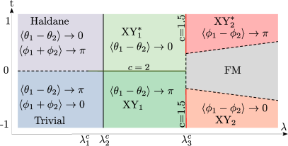
Let us begin in the limit in Eq. 81 when is irrelevant, giving us a theory. Recall that one of the two operators or is always relevant and, therefore, for , the theory flows to either a gapless state with or gaps out completely. We are interested in the case where the system does not gap out completely which occurs when is irrelevant and the theory flows to effective single-component Luttinger liquid gapless phases. The nature of the phase depends on (i) which among and dominates at large distances, pinning or and (ii) the sign of which determines the value to which the fields are pinned or . We label these four cases XY1,2 and XY as shown in Fig. 15. All four are distinct phases. The universality class of a direct continuous transition between XY1/2 and XY is the parent theory obtained by tuning . The transition between XY1 and XY2 or between XY and XY corresponds to a compact boson plus Ising CFT with central charge [86, 40, 23]. In the parameter regime we study the model numerically, a direct transition between XY2 and XY is not observed.
When we are in the XY1 or XY phases where pins the value of , a transition to a gapped phase can occur when also becomes relevant. The gapped phases resulting when and are pinned correspond to the Haldane or trivial phase [27] as shown in Fig. 15. A different transition can occur when we are in any of the four gapless phases, XY1,2 and XY and the Luttinger velocity vanishes, resulting in a first-order transition to a FM similar to the single-component small- case.
B.2.2 The line and its proximate phases
We now analyze the line and its proximity in detail. First, let us analyse which gapless phase results when is switched on. This is determined by which operator or has the smaller scaling dimension. In the parameter regime we studied numerically, we only find the former situation as shown in Fig. 15. When becomes relevant along with , we see that results in gapped phases. Let us denote as the location along the line when is marginal, i.e. where the XY1 to the trivial phase boundary and the XY -to- Haldane phase boundary meets the line at .
Now, as seen in Eq. 81, the theory is destroyed by either (i) the composite operator becomes relevant leading to a gapped state with two degenerate vaccua or (ii) the Luttinger velocity for one of the sectors vanishes rendering the continuum description invalid and we get a first-order transition to a FM. Let us denote the critical values of that result in each of these as and respectively. From the perturbative result shown in Eq. 82, we can get rough estimates for although these estimates are not very reliable when they result in large values of where the validity of perturbation theory no longer holds.
The nature of the phase transition between the trivial and Haldane phases that occurs at depends on whether we are at or . As shown in Fig. 15, the latter results in a first-order phase transition in which the vacua of the Haldane and the trivial phase are degenerate whereas the former results in a second-order transition with . Putting all this together, we get the form shown in Fig. 15.
B.2.3 Multiversality
A curious observation is that although the small- and large- gapped Haldane and trivial phases are adiabatically connected, the nature of the second-order transitions between them is different at small- and large-. For small , it is a critical theory whereas for large- it is . Both are obtained by tuning a single parameter and are therefore generic. This phenomenon, called multiversality, has received attention in recent studies [22, 23] although microscopic models that exhibit them are rare.
B.2.4 A nice possible proximate phase diagram
 |
In the parameter regime when is irrelevant, we previously argued that close to the line resulted in a gapless XY1 or (t0) XY (t0) phases if and XY2 (t0) or XY (t0) phases if . If the c=2 theory survived as (at some putative value , say) then it would open a direct transition between the phases XY2 and XY. The lines discussed previously that separated the phases XY1 and XY2 (t0) and XY and XY (t0) would meet the line at this point . Alternatively, the gapless theory becomes unstable before this can happen, giving us the situation shown in Fig. 15 which we observe in our numerical investigation. We postulate that there is some proximate parameter regime of our microscopic Hamiltonian where can be realized. In this case, we should see a phase diagram as shown in Fig. 16 which contains all the same phases as in Fig. 15 but also a direct transition between XY2 and XY.
Appendix C Bosonizing string operators
C.1 Bosonizing for small
Bosonizing string order parameters is known to be tricky and rife with ambiguities [87, 88]. Let us try to naively apply Eq. 5 to bosonize the string operator in Eq. 19 in the small - limit.
| (84) |
Equation 84 leads to the conclusion that anytime , in particular both in the Haldane and in the trivial phases. This is incorrect. We now use symmetries to identify the correct bosonized form of . We begin by postulating the following general bosonized form for
| (85) | ||||
| (86) |
While the form in Eq. 92 appears as though the string operator has been written in terms of local operators with support at and , this is not so. The half-integer prefactor to the fields ensures that the operators in are not part of the spectrum of local operators and are therefore nonlocal. Furthermore, we have used the fact that to restrict the coefficients to multiples of . We now impose constraints on using symmetry. First, observe that the end-points of defined in terms of spin operators as shown in Eq. 19 are charged under (). Using the action of on the boson fields shown in Table 2, we obtain a constraint on as
| (87) |
We now impose the action of shown in Table 7 on the bosonized form of using Table 2 which gives a relationship between and as
| (88) |
Using Eqs. 87 and 88 in Eq. 86, we get the final bosonized form for with and
| (89) |
where the coefficients are linear combinations of . This correctly reproduces the numerically observed behaviour of , which is nonzero when such as in the Haldane phase but not when such as in the trivial phase.
C.2 Bosonizing for large
We now bosonize the string operator in the large- version. We follow the same line of reasoning as shown previously for the small version. Let us begin by attempting to bosonize using the formulas shown in Eq. 9:
| (90) |
We may just as well have gone a different route to get
| (91) |
The bosonized expressions in Eqs. 90 and 91 lead to very different physics. We have when according to Eq. 90 and when according to Eq. 91 which corresponds to very different phases as seen in Fig. 15. Now we use symmetries to write down the correct bosonized form of . We again begin by postulating the following form for
| (92) | ||||
| (93) |
We now impose constraints on using symmetry. First, we use the fact that the end-points of are charged under (). Using the action of on the boson fields shown in Table 2, we get
| (94) |
We now impose the action of shown in Table 7 on the bosonized form of using Table 2 which gives a relationship between and as
| (95) |
Equations 94 and 95 are mutually compatible for non-zero iff is even. Note that we have allowed a sign ambiguity in the action of , which results in a harmless overall multiplicative sign factor in the final answer. Using these in Eq. 93, we obtain the final bosonized form of with and
| (96) |
where we have only shown operators with the smallest scaling dimensions and the coefficients are linear combinations of . This reproduces the observations in Section V that when i.e. in the Haldane and XY phases.
C.3 Bosonizing
We can obtain the bosonized form of the symmetry operator defined on a finite interval , used in the main text using arguments similar to the above by treating it as a string operator defined for any interval. In the small- limit, we can postulate the following form
| (97) | ||||
| (98) |
Unlike which has charged end-points, do not carry any charge. Thus, we have
| (99) |
Imposing the action under , we get
| (100) |
| (101) |
where we have shown only the operator with the smallest scaling dimensions, and is some combination of . In the large limit, we can postulate the form
| (102) | ||||
| (103) |
Again, imposing invariance of the endpoints, we get
| (104) |
The action of further gives us
| (105) |
Again, Eqs. 104 and 105 are mutually compatible for non-zero B iff is even and we have retained the sign ambiguity in the action of as before when we bosonized . Using these in Eq. 97, we get the final form with and
| (106) |
where we have only shown operators with the smallest scaling dimensions, and the coefficients are linear combinations of .
References
- Landau and Lifshitz [2013] L. D. Landau and E. M. Lifshitz, Statistical Physics: Volume 5, Vol. 5 (Elsevier, 2013).
- Wen [1990] X.-G. Wen, Topological orders in rigid states, International Journal of Modern Physics B 4, 239 (1990).
- Cage et al. [2012] M. E. Cage, K. Klitzing, A. Chang, F. Duncan, M. Haldane, R. B. Laughlin, A. Pruisken, and D. Thouless, The quantum Hall effect (Springer Science & Business Media, 2012).
- Haldane [2017] F. D. M. Haldane, Nobel lecture: Topological quantum matter, Rev. Mod. Phys. 89, 040502 (2017).
- Lifshitz and Pitaevskii [2013] E. M. Lifshitz and L. P. Pitaevskii, Statistical physics: theory of the condensed state, Vol. 9 (Elsevier, 2013).
- Wehling et al. [2014] T. Wehling, A. Black-Schaffer, and A. Balatsky, Dirac materials, Advances in Physics 63, 1 (2014), https://doi.org/10.1080/00018732.2014.927109 .
- Burkov [2018] A. Burkov, Weyl metals, Annual Review of Condensed Matter Physics 9, 359 (2018), https://doi.org/10.1146/annurev-conmatphys-033117-054129 .
- Sachdev [2018] S. Sachdev, Topological order, emergent gauge fields, and fermi surface reconstruction, Reports on Progress in Physics 82, 014001 (2018).
- Schulz [1995] H. J. Schulz, Fermi liquids and non–fermi liquids (1995), arXiv:cond-mat/9503150 [cond-mat] .
- Kestner et al. [2011] J. P. Kestner, B. Wang, J. D. Sau, and S. Das Sarma, Prediction of a gapless topological haldane liquid phase in a one-dimensional cold polar molecular lattice, Phys. Rev. B 83, 174409 (2011).
- Fidkowski et al. [2011] L. Fidkowski, R. M. Lutchyn, C. Nayak, and M. P. A. Fisher, Majorana zero modes in one-dimensional quantum wires without long-ranged superconducting order, Phys. Rev. B 84, 195436 (2011).
- Cheng and Tu [2011] M. Cheng and H.-H. Tu, Majorana edge states in interacting two-chain ladders of fermions, Phys. Rev. B 84, 094503 (2011).
- Ruhman et al. [2012] J. Ruhman, E. G. Dalla Torre, S. D. Huber, and E. Altman, Nonlocal order in elongated dipolar gases, Phys. Rev. B 85, 125121 (2012).
- Keselman and Berg [2015] A. Keselman and E. Berg, Gapless symmetry-protected topological phase of fermions in one dimension, Phys. Rev. B 91, 235309 (2015).
- Scaffidi et al. [2017] T. Scaffidi, D. E. Parker, and R. Vasseur, Gapless symmetry-protected topological order, Phys. Rev. X 7, 041048 (2017).
- Parker et al. [2018] D. E. Parker, T. Scaffidi, and R. Vasseur, Topological luttinger liquids from decorated domain walls, Phys. Rev. B 97, 165114 (2018).
- Jiang et al. [2018] H.-C. Jiang, Z.-X. Li, A. Seidel, and D.-H. Lee, Symmetry protected topological luttinger liquids and the phase transition between them, Science Bulletin 63, 753 (2018).
- Verresen et al. [2021] R. Verresen, R. Thorngren, N. G. Jones, and F. Pollmann, Gapless topological phases and symmetry-enriched quantum criticality, Phys. Rev. X 11, 041059 (2021).
- Thorngren et al. [2021] R. Thorngren, A. Vishwanath, and R. Verresen, Intrinsically gapless topological phases, Phys. Rev. B 104, 075132 (2021).
- Haldane [1981a] F. D. M. Haldane, Luttinger liquid theory of one-dimensional quantum fluids. i. properties of the luttinger model and their extension to the general 1d interacting spinless fermi gas, Journal of Physics C: Solid State Physics 14, 2585 (1981a).
- Ginsparg [1988] P. Ginsparg, Applied conformal field theory, (1988), arXiv:hep-th/9108028 [hep-th] .
- Bi and Senthil [2019] Z. Bi and T. Senthil, Adventure in topological phase transitions in -d: Non-abelian deconfined quantum criticalities and a possible duality, Phys. Rev. X 9, 021034 (2019).
- Prakash et al. [2023] A. Prakash, M. Fava, and S. A. Parameswaran, Multiversality and unnecessary criticality in one dimension, Phys. Rev. Lett. 130, 256401 (2023).
- Kohmoto et al. [1981] M. Kohmoto, M. den Nijs, and L. P. Kadanoff, Hamiltonian studies of the ashkin-teller model, Phys. Rev. B 24, 5229 (1981).
- Haldane [1982] F. D. M. Haldane, Spontaneous dimerization in the heisenberg antiferromagnetic chain with competing interactions, Phys. Rev. B 25, 4925 (1982).
- Strong and Millis [1992] S. P. Strong and A. J. Millis, Competition between singlet formation and magnetic ordering in one-dimensional spin systems, Phys. Rev. Lett. 69, 2419 (1992).
- Orignac and Giamarchi [1998] E. Orignac and T. Giamarchi, Weakly disordered spin ladders, Phys. Rev. B 57, 5812 (1998).
- Somma and Aligia [2001] R. D. Somma and A. A. Aligia, Phase diagram of the xxz chain with next-nearest-neighbor interactions, Phys. Rev. B 64, 024410 (2001).
- Hirata and Nomura [2000] S. Hirata and K. Nomura, Phase diagram of chain with next-nearest-neighbor interaction, Phys. Rev. B 61, 9453 (2000).
- Jiang et al. [2002] X.-F. Jiang, Q. Jiang, and D. Xing, Elementary excitation and ground-state properties of dimerized xxz chain with frustration, physica status solidi (b) 229, 1451 (2002).
- Furukawa et al. [2012] S. Furukawa, M. Sato, S. Onoda, and A. Furusaki, Ground-state phase diagram of a spin- frustrated ferromagnetic xxz chain: Haldane dimer phase and gapped/gapless chiral phases, Phys. Rev. B 86, 094417 (2012).
- Sato et al. [2011] M. Sato, S. Furukawa, S. Onoda, and A. Furusaki, Competing phases in spin- j1-j2 chain with easy-plane anisotropy, Modern Physics Letters B 25, 901 (2011).
- Note [1] The and symmetries do not commute and together form the non-abelian group .
- Chen et al. [2011] X. Chen, Z.-C. Gu, and X.-G. Wen, Complete classification of one-dimensional gapped quantum phases in interacting spin systems, Phys. Rev. B 84, 235128 (2011).
- Giamarchi [2004] T. Giamarchi, Quantum physics in one dimension, International series of monographs on physics (Clarendon Press, Oxford, 2004).
- Haldane [1981b] F. Haldane, Demonstration of the “luttinger liquid” character of bethe-ansatz-soluble models of 1-d quantum fluids, Physics Letters A 81, 153 (1981b).
- Francesco et al. [2012] P. Francesco, P. Mathieu, and D. Sénéchal, Conformal field theory (Springer Science & Business Media, 2012).
- Note [2] Recall that a scaling operator is relevant in d+1 dimensions if its scaling dimensions satisfies .
- Nersesyan et al. [1998] A. A. Nersesyan, A. O. Gogolin, and F. H. L. Eßler, Incommensurate spin correlations in spin- frustrated two-leg heisenberg ladders, Phys. Rev. Lett. 81, 910 (1998).
- Schulz [1986] H. J. Schulz, Phase diagrams and correlation exponents for quantum spin chains of arbitrary spin quantum number, Phys. Rev. B 34, 6372 (1986).
- He et al. [2023] Y. He, D. M. Kennes, C. Karrasch, and R. Rausch, Terminable transitions in a topological fermionic ladder, (2023), arXiv:2302.14085 [cond-mat.str-el] .
- He et al. [2021] Y. He, D. Pekker, and R. S. K. Mong, One-dimensional repulsive hubbard model with mass imbalance: Orders and filling anomaly, Phys. Rev. B 104, 195126 (2021).
- Note [3] The two symmetries also contains a well known mixed anomaly [89]. The full collection of symmetries of the compact boson CFT is larger and contains the group of conformal transformations as well as other generators that may not even form a group structure [90, 91]. For our purposes, the ones listed in Eq. 11 that form are sufficient.
- Note [4] Note that lattice operators with charge 2 such as will have algebraic correlations in XY2 and XY phases as shown in [40].
- Li et al. [2022] L. Li, M. Oshikawa, and Y. Zheng, Symmetry protected topological criticality: Decorated defect construction, signatures and stability, (2022), arXiv:2204.03131 [cond-mat.str-el] .
- Wen and Potter [2023] R. Wen and A. C. Potter, Bulk-boundary correspondence for intrinsically gapless symmetry-protected topological phases from group cohomology, Phys. Rev. B 107, 245127 (2023).
- Note [5] Note that Eq. 43 that breaks but preserves can be introduced to eliminate XY but preserve the Haldane phase. But this is not interesting.
- Chen et al. [2013] X. Chen, Z.-C. Gu, Z.-X. Liu, and X.-G. Wen, Symmetry protected topological orders and the group cohomology of their symmetry group, Phys. Rev. B 87, 155114 (2013).
- White [1992] S. R. White, Density matrix formulation for quantum renormalization groups, Phys. Rev. Lett. 69, 2863 (1992).
- Schollwöck [2011] U. Schollwöck, The density-matrix renormalization group in the age of matrix product states, Annals of Physics 326, 96 (2011), january 2011 Special Issue.
- Schollwöck [2005] U. Schollwöck, The density-matrix renormalization group, Rev. Mod. Phys. 77, 259 (2005).
- Yoshida and Okamoto [1989] S. Yoshida and K. Okamoto, Phase diagram of spin-1/2 alternating ferromagnetic chain with xy-like anisotropy, Journal of the Physical Society of Japan 58, 4367 (1989), https://doi.org/10.1143/JPSJ.58.4367 .
- Mishra et al. [2015] T. Mishra, S. Greschner, and L. Santos, Frustration-induced supersolids in the absence of intersite interactions, Phys. Rev. B 92, 195149 (2015).
- Greschner and Mishra [2019] S. Greschner and T. Mishra, Interacting bosons in generalized zigzag and railroad-trestle models, Phys. Rev. B 100, 144405 (2019).
- Dhar et al. [2012] A. Dhar, M. Maji, T. Mishra, R. V. Pai, S. Mukerjee, and A. Paramekanti, Bose-hubbard model in a strong effective magnetic field: Emergence of a chiral mott insulator ground state, Phys. Rev. A 85, 041602 (2012).
- Mondal et al. [2019] S. Mondal, S. Greschner, and T. Mishra, Three-body constrained bosons in a double-well optical lattice, Phys. Rev. A 100, 013627 (2019).
- Mishra et al. [2011] T. Mishra, J. Carrasquilla, and M. Rigol, Phase diagram of the half-filled one-dimensional -- model, Phys. Rev. B 84, 115135 (2011).
- Mondal et al. [2022] S. Mondal, A. Padhan, and T. Mishra, Realizing a symmetry protected topological phase through dimerized interactions, Phys. Rev. B 106, L201106 (2022).
- [59] S.-J. GU, Fidelity approach to quantum phase transitions, International Journal of Modern Physics B , 4371.
- Singh et al. [2018] M. Singh, S. Greschner, and T. Mishra, Anomalous pairing of bosons: Effect of multibody interactions in an optical lattice, Phys. Rev. A 98, 023615 (2018).
- Lahiri et al. [2020] S. Lahiri, S. Mondal, K. Pandey, and T. Mishra, Correlated photon pair propagation in circuit qed with superconducting processors, Phys. Rev. A 102, 043710 (2020).
- Calabrese and Cardy [2009] P. Calabrese and J. Cardy, Entanglement entropy and conformal field theory, Journal of physics a: mathematical and theoretical 42, 504005 (2009).
- Hida [1992] K. Hida, Crossover between the haldane-gap phase and the dimer phase in the spin-1/2 alternating heisenberg chain, Phys. Rev. B 45, 2207 (1992).
- Chen et al. [2003] W. Chen, K. Hida, and B. C. Sanctuary, Ground-state phase diagram of chains with uniaxial single-ion-type anisotropy, Phys. Rev. B 67, 104401 (2003).
- Affleck [2008] I. Affleck, Quantum impurity problems in condensed matter physics 10.48550/ARXIV.0809.3474 (2008).
- Yu et al. [2022] X.-J. Yu, R.-Z. Huang, H.-H. Song, L. Xu, C. Ding, and L. Zhang, Conformal boundary conditions of symmetry-enriched quantum critical spin chains, Phys. Rev. Lett. 129, 210601 (2022).
- Cabra et al. [1998] D. C. Cabra, A. Honecker, and P. Pujol, Magnetization plateaux in -leg spin ladders, Phys. Rev. B 58, 6241 (1998).
- Cabra et al. [1997] D. C. Cabra, A. Honecker, and P. Pujol, Magnetization curves of antiferromagnetic heisenberg spin- ladders, Phys. Rev. Lett. 79, 5126 (1997).
- Mukhopadhyay et al. [2001] R. Mukhopadhyay, C. L. Kane, and T. C. Lubensky, Sliding luttinger liquid phases, Phys. Rev. B 64, 045120 (2001).
- Sondhi and Yang [2001] S. L. Sondhi and K. Yang, Sliding phases via magnetic fields, Phys. Rev. B 63, 054430 (2001).
- Emery et al. [2000] V. J. Emery, E. Fradkin, S. A. Kivelson, and T. C. Lubensky, Quantum theory of the smectic metal state in stripe phases, Phys. Rev. Lett. 85, 2160 (2000).
- Vishwanath and Carpentier [2001] A. Vishwanath and D. Carpentier, Two-dimensional anisotropic non-fermi-liquid phase of coupled luttinger liquids, Phys. Rev. Lett. 86, 676 (2001).
- Yakovenko [1991] V. M. Yakovenko, Quantum hall effect in quasi-one-dimensional conductors, Phys. Rev. B 43, 11353 (1991).
- Neupert et al. [2014] T. Neupert, C. Chamon, C. Mudry, and R. Thomale, Wire deconstructionism of two-dimensional topological phases, Phys. Rev. B 90, 205101 (2014).
- Meng et al. [2015] T. Meng, T. Neupert, M. Greiter, and R. Thomale, Coupled-wire construction of chiral spin liquids, Phys. Rev. B 91, 241106 (2015).
- Liu et al. [2023] Y. Liu, N. Tantivasadakarn, K. Slagle, D. F. Mross, and J. Alicea, Assembling kitaev honeycomb spin liquids from arrays of 1d symmetry protected topological phases (2023), arXiv:2305.11221 [cond-mat.str-el] .
- Morgado and Whitlock [2021] M. Morgado and S. Whitlock, Quantum simulation and computing with Rydberg-interacting qubits, AVS Quantum Science 3, 023501 (2021), https://pubs.aip.org/avs/aqs/article-pdf/doi/10.1116/5.0036562/14572456/023501_1_online.pdf .
- Tsitsishvili et al. [2022] M. Tsitsishvili, T. Chanda, M. Votto, P. Fromholz, M. Dalmonte, and A. Nersesyan, Phase diagram of rydberg-dressed atoms on two-leg square ladders: Coupling supersymmetric conformal field theories on the lattice, Phys. Rev. B 105, 155159 (2022).
- Eck and Fendley [2023a] L. Eck and P. Fendley, From the xxz chain to the integrable rydberg-blockade ladder via non-invertible duality defects, (2023a), arXiv:2302.14081 [cond-mat.stat-mech] .
- Eck and Fendley [2023b] L. Eck and P. Fendley, Critical lines and ordered phases in a rydberg-blockade ladder, (2023b), arXiv:2304.08484 [cond-mat.str-el] .
- Fromholz et al. [2022] P. Fromholz, M. Tsitsishvili, M. Votto, M. Dalmonte, A. Nersesyan, and T. Chanda, Phase diagram of rydberg-dressed atoms on two-leg triangular ladders, Phys. Rev. B 106, 155411 (2022).
- Orbach [1958] R. Orbach, Linear antiferromagnetic chain with anisotropic coupling, Phys. Rev. 112, 309 (1958).
- Yang and Yang [1966a] C. N. Yang and C. P. Yang, One-dimensional chain of anisotropic spin-spin interactions. i. proof of bethe’s hypothesis for ground state in a finite system, Phys. Rev. 150, 321 (1966a).
- Yang and Yang [1966b] C. N. Yang and C. P. Yang, One-dimensional chain of anisotropic spin-spin interactions. ii. properties of the ground-state energy per lattice site for an infinite system, Phys. Rev. 150, 327 (1966b).
- Delfino and Mussardo [1998] G. Delfino and G. Mussardo, Non-integrable aspects of the multi-frequency sine-gordon model, Nuclear Physics B 516, 675 (1998).
- Lecheminant et al. [2002] P. Lecheminant, A. O. Gogolin, and A. A. Nersesyan, Criticality in self-dual sine-gordon models, Nuclear Physics B 639, 502 (2002).
- Kim et al. [2000] E. H. Kim, G. Fáth, J. Sólyom, and D. J. Scalapino, Phase transitions between topologically distinct gapped phases in isotropic spin ladders, Phys. Rev. B 62, 14965 (2000).
- Nakamura [2003] M. Nakamura, Identification of topologically different valence bond states in spin ladders, Physica B: Condensed Matter 329-333, 1000 (2003), proceedings of the 23rd International Conference on Low Temperature Physics.
- Fradkin [2021] E. Fradkin, Quantum field theory: an integrated approach (Princeton University Press, 2021).
- Thorngren and Wang [2021] R. Thorngren and Y. Wang, Fusion category symmetry ii: Categoriosities at c = 1 and beyond, (2021), arXiv:2106.12577 [hep-th] .
- Choi et al. [2022] Y. Choi, C. Córdova, P.-S. Hsin, H. T. Lam, and S.-H. Shao, Noninvertible duality defects in dimensions, Phys. Rev. D 105, 125016 (2022).