Surface sensitivity of magnetization in the mesoscopic regime

Abstract

We find that in the mesoscopic regime modification of the material’s surface can induce an extensive change of the material’s magnetic moment. In other words, perturbation of order $N^{2}$ atoms on the surface of a 3-dimensional solid can change the magnetic moment proportionally to $N^{3}$. When the solid’s surface is perturbed, it triggers two changes in the magnetization. One arises from variations of the electron wavefunction and energy, while the other arises from a modification in the kinetic angular momentum operator. In the macroscopic regime of our model, these two bulk effects cancel each other, resulting in no impact of the surface perturbation on the magnetization — consistent with prior work. In the mesoscopic regime, we find a departure from this behavior, as the cancelation of two terms is not complete.

In a ferromagnet, the magnetic moment primarily arises from the unequal population of electrons with different spin states. A smaller, but significant contribution, known as orbital magnetization, originates from the microscopic spatial motion of electrons throughout the material. Some of these microscopic orbital electron currents flow around individual atoms in the bulk, while other currents traverse the surface of the sample, as demonstrated in Ref. 1 using a framework of localized Wannier states. Although only a fraction of electrons participate in surface currents, their collective effect contributes to the magnetic dipole moment, scaling with the volume of the sample (area in two dimensions).

The question then arises whether the magnetic moment of the ferromagnet could be modified by perturbing surface of the material? For instance, one may wonder if adsorbing atoms to the surface of a solid could induce currents and consequently change the magnetic dipole of the solid, in proportion to the volume of the solid? In other words, we are asking whether perturbing order $N^{2}$ atoms on the surface of a 3-dimensional solid could change the magnetic moment proportional to $N^{3}$? Or, similarly, whether perturbing order $N$ atoms on the edge of a 2-dimensional solid could change the magnetic moment in proportion to $N^{2}$?

The seminal work from Ref. 1 demonstrated that none of these scenarios are possible for insulating systems. In an insulating system, the surface currents are quite remarkably determined by the material properties deep in the bulk of the material! Intuitively, one would expect such a statement to also extend to metallic cases. Reference 2 gives heuristic reasons why magnetization in a metal is equally well determined by the properties of the bulk of the material, as in the case of an insulator. (The same was also suggested for topological insulators in Refs. 2, 3, 4.) Additional support is given by the semiclassical formulation of orbital magnetization from Ref. 5 as well as the long-wave perturbation from Ref. 6. A more recent proof that orbital magnetization in a metal is a bulk property relies on a local measure of the orbital moment from Refs. 7, 8, 9.

In this paper, our focus lies on a distinct range of length and temperature scales, one that complements the scope of previous investigations. Previous studies can be applied to the macroscopic regime, which we define as,

$$\frac{L}{v_{\rm F}}\gg\frac{\hbar}{k_{\rm B}T}.$$ (1)

Here $v_{\rm F}$ is the electron’s Fermi velocity and $L$ is a length of the sample. In other words, in the macroscopic regime, the electron’s time of flight across the sample ($L/v_{\rm F}$) exceeds the time scale associated with the thermal energy $k_{\rm B}T$. In the macroscopic regime our findings corroborate the conclusions drawn in Refs. 5, 1, 2, 6, 3, 7, 8, 9, 4. Specifically, the surface modifications does not lead to extensive change in the magnetization.

Nevertheless, an intriguing situation emerges when we shift to the opposite regime,

$$\frac{L}{v_{\rm F}}<\frac{\hbar}{k_{\rm B}T},$$ (2)

which we refer to as the mesoscopic regime. Our work shows that in the mesoscopic regime the surface can indeed change the overall magnetic moment of the sample, in proportion to the volume of the sample.

Before introducing our numerical model, we first motivate it by considering a continuous one-particle effective Hamiltonian, denoted $H^{0}_{\rm c}$, for a periodic infinite solid. For simplicity we work in two dimensions, but generalization to higher dimensions is straightforward. When dealing with the two-dimensional models, we will refer to the boundary of this model as edge instead of surface, which we reserve for three-dimensional solids. To simplify our analysis, throughout this work we neglect spin, self-consistency, many-electron effects, and disorder. Our system is assumed to be in thermal equilibrium. We ignore any temperature effects beyond electron occupation smearing.

The complete basis of the eigenstates of $H^{0}_{\rm c}$ can be expressed in the Bloch form, $\psi_{\bm{k}}({\bm{r}})=e^{i{\bm{k}}\cdot{\bm{r}}}u_{\bm{k}}({\bm{r}})$. However, not every eigenstate of $H^{0}_{\rm c}$ has the Bloch form. Generally, we can construct arbitrary linear combinations of states that share the same eigenvalue $E_{\bm{k}}=E$, and the resulting function

$$\phi_{E}({\bm{r}})=\int_{0}^{1}e^{if(s)}\psi_{\bm{k}(s)}({\bm{r}})ds$$ (3)

is a valid eigenstate of $H^{0}_{\rm c}$. Here $s\rightarrow{\bm{k}}(s)$ is a continuous parameterization of a curve in the Brillouin zone along which $E_{{\bm{k}}(s)}=E$. For now we limit $f(s)$ so that $f(0)=f(1)$. We choose $f(s)$ so that $\phi_{E}({\bm{r}})$ is as localized as possible in the real space. By selecting a fixed $f(s)$, we create a family of functions, $\phi_{mE}$, for any integer $m$, defined as follows,

$$\phi_{mE}({\bm{r}})=\int_{0}^{1}e^{i2\pi ms}e^{if(s)}\psi_{\bm{k}(s)}({\bm{r}})ds.$$ (4)

Note, trivially, that $\braket{\phi_{mE}}{\phi_{m^{\prime}E^{\prime}}}=\delta_{mm^{\prime}}\delta_{EE^{\prime}}$. Therefore, $\phi_{mE}$ for all $m$ and $E$ span the same vector space as the Bloch states. Let us now take $H^{0}_{\rm c}$ to correspond to the free-electron system with mass $m_{\rm e}$. In this case $\phi_{mE}({\bm{r}})$ in cylindrical coordinates is simply $\sim e^{im\varphi}J_{m}\left(\frac{\sqrt{2m_{\rm e}E}}{\hbar}r\right)$. Here $J_{m}$ is the Bessel function of the first kind.

Trivially, the expectation value of the angular momentum operator $L_{z}$ is

$$\bra{\phi_{mE}}L_{z}\ket{\phi_{mE}}=\hbar m.$$ (5)

Therefore, each state $\phi_{mE}$ carries angular momentum $\hbar m$, and orbital magnetic moment $\mu_{\rm B}m$. Let us now confine our system to a circular region with radius $R$. From elementary properties of Bessel functions it follows that states with large enough $m$, close to $R\frac{\sqrt{2m_{\rm e}E}}{\hbar}$, are localized near the edge of the sample ($r\approx R$). Edge states therefore carry an angular momentum $\hbar m\sim R^{1}$. The number of states near the edge also scales as $\sim R^{1}$. Therefore, one might ask whether tweaking the electron potential $V^{\rm edge}$ near the edge of the sample could modify edge states and induce a net orbital moment that scales as $\sim R^{2}$? If one could construct an edge potential $V^{\rm edge}$ satisfying

$$\bra{\phi_{mE}}V^{\rm edge}\ket{\phi_{m^{\prime}E}}\sim m\delta_{mm^{\prime}}$$ (6)

then this would be a good candidate edge perturbation, as it breaks the time-reversal symmetry by differently acting on state with different $m$. For example, one of the effects of this perturbation would be to push $m<0$ states below the Fermi level, and $m>0$ states above the Fermi level, thus inducing a net magnetic dipole.

We now attempt to create edge potential satisfying Eq. 6 in a concrete finite-size model using a numerically convenient tight-binding approach. To construct the tight-binding model, we project our continuous free-electron Hamiltonian $H^{0}_{\rm c}$ on the basis of a $N\times N$ square mesh of s-like orbitals separated by a distance $a$ (orbitals are sketched as black circles in Fig. 1). We label the orbital at site $i$ as $\ket{i}$. For the position operators $x$ and $y$, we assume $\bra{i}x\ket{j}=x_{i}\delta_{ij}$ and $\bra{i}y\ket{j}=y_{i}\delta_{ij}$. For convenience, we work with the centered operators $\tilde{x}=x-\sum_{i}x_{i}/N^{2}$ and $\tilde{y}=y-\sum_{i}y_{i}/N^{2}$. We also define the following quantity $\tilde{L}(A)$ for any operator $A$,

$$\tilde{L}(A) =\frac{im_{\rm e}}{\hbar}\left(\tilde{x}[A,\tilde{y}]-\tilde{y}[A,\tilde{x}]\right)$$

$$=\frac{im_{\rm e}}{\hbar}\left(\tilde{x}A\tilde{y}-\tilde{y}A\tilde{x}\right).$$ (7)

Clearly $\tilde{L}(H)$ corresponds to the angular momentum operator for a system described by the Hamiltonian $H$.

Our general procedure to construct edge potential $V^{\rm edge}$ for any bulk hamiltonian $H^{0}$ consists of the following five steps.

$${\rm Step\ 1:\ choose\ }H^{0}.$$

$${\rm Step\ 2:\ construct\ }H^{\rm comm}{\rm\ from\ }H^{0}.$$

$${\rm Step\ 3:\ construct\ }V^{\rm edge}{\rm\ from\ }\tilde{L}(H^{0}).$$

$${\rm Step\ 4:\ diagonalize\ }H=H^{0}+H^{\rm comm}+V^{\rm edge}.$$

$${\rm Step\ 5:\ compute\ }m_{\rm dip}=\frac{e}{2m_{\rm e}}\sum_{n}\bra{\psi_{n}}\tilde{L}(H)\ket{\psi_{n}}f_{n}.$$

In step 1 of our procedure, for now we choose the simplest $H^{0}$, where $H^{0}_{ij}=\bra{i}H^{0}\ket{j}=t<0$ for the nearest-neighbor orbitals $i$ and $j$, and $0$ for any other pair of orbitals (represented by black lines in Fig. 1).

Now we want to construct an edge potential with the property given in Eq. 6. At first it is not clear how to satisfy Eq. 6 in our model, as eigenvectors of $H^{0}$ don’t have a well-defined angular momentum (our tight-binding model is projected into a finite square mesh of orbitals which breaks continuous rotational symmetry). Therefore, before discussing the edge perturbation, we in step 2 of our procedure, construct a commutator correction term $H^{\rm comm}$ which ensures that total bulk Hamiltonian,

$$H^{\rm bulk}=H^{0}+H^{\rm comm},$$ (8)

at least approximately commutes with the angular momentum operator, $\tilde{L}(H^{\rm bulk})$. The straightforward but tedious construction of $H^{\rm comm}$ is given in the supplement.

The energy spectrum of $H^{0}$ as a function of $N$ exhibits some regularity by having spikes in the density of states separated by $\Delta\sim 1/N$. However, the number of states in between spikes is not strictly zero, and these states don’t follow an obvious pattern as a function of increasing $N$. If we include the $H^{\rm comm}$ in our Hamiltonian, we find that it redistributes the spectrum of the system, creating small gaps in the spectrum (scaling as $\Delta\sim 1/N$), as shown in the supplement. We find that placing a Fermi level $E_{\rm F}$ within one of these gaps has the additional benefit of stabilizing the finite-size effects in our calculations. Related finite-size effects for Landau diamagnetism have also been reported in Refs. 14, 15, 16, 17, 18.

Step 3: we now construct edge perturbation

$$V^{\rm edge}_{ij}=-\frac{eB}{2m_{\rm e}}S_{ij}\tilde{L}_{ij}(H^{0}).$$ (9)

This term introduces complex phases to the hopping elements on the edge of the model. See panel (a) of Fig. 1 for a sketch of the alternating magnetic flux applied to the edge of the sample.

The $S_{ij}$ term in Eq. 9 ensures that the perturbing potential $V^{\rm edge}$ is zero in the bulk and non-zero only on the edges. Without including $S_{ij}$ in $V^{\rm edge}$, the resulting $V^{\rm edge}_{ij}$ would represent an approximate interaction term of the orbital magnetic moment with a spatially uniform external magnetic field $B$, as in the study of Landau diamagnetism. Trivially, the matrix element of such a perturbation is proportional to $m$, as in Eq. 6.

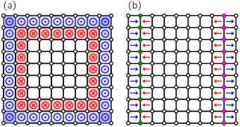
Figure 1: (a) Perturbation $V^{\rm edge}$, given by Eq. 9, induces complex phases on hopping elements near the edge. Blue and red colors represent different signs of effective local magnetic field on the edge. (b) Perturbation $V^{\prime\rm edge}$, given by Eq. 16, changes the onsite energies of green and purple orbitals on the left and right edges. Arrows represent directions of effective local electric field at the edge. In both cases (a) and (b) magnitude of effective magnetic and electric fields on the edge is independent of $N$.

Step 4: diagonalizing our full Hamiltonian, which includes both bulk and edge contribution,

$$\left(H^{\rm bulk}+V^{\rm edge}\right)\ket{\psi_{n}}=E_{n}\ket{\psi_{n}}$$ (10)

we obtain a set of eigenstates $\ket{\psi_{n}}$. The largest model we used has $N=100$, corresponding to a system with 10,000 orbitals. We set the Fermi level $E_{\rm F}$ to $-2.55\,|t|$, placing it within a small energy gap $\Delta$ in the spectrum.

Step 5: the magnetic dipole moment we compute as

$$m_{\rm dip} =\frac{e}{2m_{\rm e}}\sum_{n}\bra{\psi_{n}}\tilde{L}(H)\ket{\psi_{n}}f_{n}.$$ (11)

Here $f_{n}$ is the Fermi-Dirac distribution with effective smearing of electron occupation by $k_{\rm B}T$. Figure 2 shows the calculated $m_{\rm dip}$ as a function of $N$. The computed $m_{\rm dip}$ is clearly extensive for our two-dimensional model, as it scales nearly perfectly as $N^{2}$.

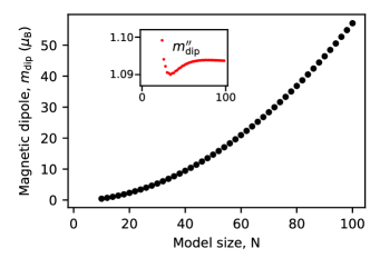
Figure 2: Changing order $N$ terms in our two-dimensional model induces $N^{2}$ change in the computed magnetic dipole $m_{\rm dip}$. Here, the temperature $k_{\rm B}T$ in the Fermi-Dirac distribution is set to $0$. $B$ is chosen so that $a^{2}B=0.2\hbar/e$. Fermi level $E_{\rm F}$ is set to $-2.55\,|t|$ so that the electron density is $\approx 0.12/a^{2}$. The parameters $t$ and $a$ are set so that the effective mass at low doping is the same as the free electron mass. The inset shows that the second derivative of $m_{\rm dip}$ with respect to $N$ (scaled by $10^{2}$) is constant.

However, as we show in the supplement, we find numerically that the $N^{2}$ scaling persists only when

$$k_{\rm B}T\lesssim 0.2\,\Delta\approx 0.6\,\frac{|t|}{N}.$$ (12)

Since $|t|\sim v_{\rm F}$ and $N\sim L$ clearly Eq. 12 is equivalent to the definition of the mesoscopic regime given by Eq. 2. In other words, $N^{2}$ scaling of $m_{\rm dip}$ in our model persists only in the mesoscopic regime.

Furthermore, we find that $m_{\rm dip}$ can be fitted well to the following functional form, either in the macroscopic or the mesoscopic regime,

$$m_{\rm dip}\sim\frac{N^{2}}{1+\exp\left[3.8\displaystyle\frac{k_{\rm B}T}{|t|}\left(N-0.6\displaystyle\frac{|t|}{k_{\rm B}T}\right)\right]}.$$ (13)

From this functional form it is clear that $m_{\rm dip}\sim N^{2}$ in the mesoscopic regime. More precisely, the following mesoscopic limit

$$\lim_{N\rightarrow\infty}\lim_{T\rightarrow 0^{+}}\frac{m_{\rm dip}}{N^{2}}\neq 0$$ (14)

is non-zero. In other words, the $N^{2}$ scaling of the magnetic moment continues for all $N$, as long as the temperature is small enough. On the other hand, if we swap the order of limits, the resulting macroscopic limit

$$\lim_{T\rightarrow 0^{+}}\lim_{N\rightarrow\infty}\frac{m_{\rm dip}}{N^{2}}=0$$ (15)

is now zero. In other words, for any fixed small positive $T$ there is an $N$ beyond which the magnetic dipole no longer scales as $N^{2}$.

In the supplementary material, we provide explicit numerical values of Hamiltonian matrix elements $H_{ij}$ for different values of $N$, as well as a computer code that diagonalizes Eq. 10, computes Eq. 11, and performs a range of consistency checks on $H_{ij}$.

In hindsight, our finding that $m_{\rm dip}$ in a metal is edge sensitive is perhaps not that surprising considering that a similar dependence was found for the electric dipole $d_{\rm dip}$ of a metal. [23] However, importantly, the electric dipole $d_{\rm dip}$ is edge sensitive in a metal even in a macroscopic regime. Therefore, we can naturally ask why, in the macroscopic regime, $m_{\rm dip}$ from our model behaves differently from $d_{\rm dip}$?

To establish a parallel between the electric and magnetic dipole, it is instructive to construct an edge potential $V^{\prime\rm edge}$ that changes the bulk electric dipole, in analogy to how $V^{\rm edge}$ changed the bulk magnetic dipole. To achieve this, we use the following procedure.

$${\rm Step\ 1^{\prime}:\ choose\ }H^{0}.$$

$${\it Step\ 2^{\prime}:\ (commutator\ correction\ term\ not\ needed.)}$$

$${\rm Step\ 3^{\prime}:\ construct\ }V^{\prime\rm edge}{\rm\ from\ }\tilde{x}.$$

$${\rm Step\ 4^{\prime}:\ diagonalize\ }H=H^{0}+V^{\prime\rm edge}.$$

$${\rm Step\ 5^{\prime}:\ compute\ }d_{\rm dip}=e\sum_{n}\bra{\psi_{n}}\tilde{x}\ket{\psi_{n}}f_{n}.$$

In step $1^{\prime}$, we take the same $H^{0}$ as before. Step $2^{\prime}$ is not needed, as we find that a numerically robust $N^{2}$ scaling of $d_{\rm dip}$ is present even without commutator correction.

The important difference is in step $3^{\prime}$. Earlier, in the case of the magnetic dipole, we constructed $V^{\rm edge}$ from the angular momentum operator $\tilde{L}(H^{0})$, which induced an effective alternating magnetic field at the edge. Now, by analogy, in step $3^{\prime}$ we construct the edge potential from the position operator,

$$V^{\prime\rm edge}_{ij}=-e{\cal E}S_{i}\tilde{x}_{i}\delta_{ij},$$ (16)

which induced effective electric fields on the edge, proportional to ${\cal E}$. Panel (b) of Fig. 1 shows the sketch of the effective electric fields near the edge induced by $V^{\prime\rm edge}$. In Eq. 16 we use $S_{i}$ to ensure that the perturbation potential $V^{\prime\rm edge}$ is zero in the bulk.

In the final step ($5^{\prime}$) of our procedure, we now compute the expectation value of the electric dipole moment, $d_{\rm dip}=e\sum_{n}\bra{\psi_{n}}\tilde{x}\ket{\psi_{n}}f_{n}.$ As shown in the supplement, we find that $d_{\rm dip}$ scales as $\sim N^{2}$, even in the macroscopic regime, as expected based on Ref. [23].

We assign a different behavior of an electrical dipole to that of a magnetic dipole due to the fact that the magnetic dipole in step $5$ is computed as a trace over operator $\tilde{L}(H)$ which explicitly includes the edge perturbation $V^{\rm edge}$ itself,

$$\tilde{L}(H)=\tilde{L}(H^{\rm bulk})+\tilde{L}(V^{\rm edge}).$$ (17)

Therefore, the magnetic dipole $m_{\rm dip}$ can be decomposed into two contributions. The first is a partial trace of $\tilde{L}(H^{\rm bulk})$

$$m_{\rm dip}^{\rm st} =\frac{e}{2m_{\rm e}}\sum_{n}\bra{\psi_{n}}\tilde{L}(H^{\rm bulk})\ket{\psi_{n}}f_{n},$$ (18)

and it arises from changes to the electron state (wavefunction and energy) due to edge perturbation $V^{\rm edge}$. The second term is a partial trace of $\tilde{L}(V^{\rm edge})$

$$m_{\rm dip}^{\rm op} =\frac{e}{2m_{\rm e}}\sum_{n}\bra{\psi_{n}}\tilde{L}(V^{\rm edge})\ket{\psi_{n}}f_{n}.$$ (19)

and it originates from the change in the angular momentum operator by inclusion of perturbation $V^{\rm edge}$ in the total Hamiltonian. This term, in the lowest order of perturbation theory, can be computed already from the unperturbed electron wavefunction and energy.

On the contrary, the electric dipole is calculated in step $5^{\prime}$ as a trace over the position operator $\tilde{x}$, which clearly does not depend on the edge perturbation $V^{\prime\rm edge}$. Therefore, the electric dipole is induced in the model only by changes in the electron wavefunction and energy (analogous to $m_{\rm dip}^{\rm st}$). In the case of the electric dipole, there are no terms analogous to $m_{\rm dip}^{\rm op}$.

Interestingly, we find that both $m_{\rm dip}^{\rm st}$ and $m_{\rm dip}^{\rm op}$ are extensive in the macroscopic regime, on their own. However, in the macroscopic regime, these two terms exactly cancel each other, resulting in a nonextensive magnetic dipole in the macroscopic regime. In contrast, in the case of the electric dipole, there is only one contribution (the one coming from changes in the electron’s state), so there is no cancelation, and the electric dipole remains edge-sensitive in the macroscopic regime.

In our work, we focus on the simplest choice of $H^{0}$, which corresponds to a square lattice with first-neighbor hoppings. However, the procedure presented in this paper can be done for any $H^{0}$. An interesting case is the Haldane model in a topologically nontrivial insulator phase with a nonzero Chern number.[25] Here, even when the Fermi level is within the bulk gap and crosses the topologically protected edge states, we find $m_{\rm dip}\sim N^{2}$. This is numerically robust even without including the commutator correction term $H^{\rm comm}$.

in 1,2,3,4,5,6,7,8,9,10 See pages \x, of supp.pdf