Disk Wind Feedback from High-mass Protostars. III. Synthetic CO Line Emission

Abstract

To test theoretical models of massive star formation it is important to compare their predictions with observed systems. To this end, we conduct CO molecular line radiative transfer post-processing of 3D magneto-hydrodynamic (MHD) simulations of various stages in the evolutionary sequence of a massive protostellar core, including its infall envelope and disk wind outflow. Synthetic position-position-velocity (PPV) cubes of various transitions of ¹²CO, ¹³CO, and C¹⁸O emission are generated. We also carry out simulated Atacama Large Millimeter/submillimeter Array (ALMA) observations of this emission. We compare the mass, momentum and kinetic energy estimates obtained from molecular lines to the true values, finding that the mass and momentum estimates can have uncertainties of up to a factor of four. However, the kinetic energy estimated from molecular lines is more significantly underestimated. Additionally, we compare the mass outflow rate and momentum outflow rate obtained from the synthetic spectra with the true values. Finally, we compare the synthetic spectra with real examples of ALMA-observed protostars and determine the best fitting protostellar masses and outflow inclination angles. We then calculate the mass outflow rate and momentum outflow rate for these sources, finding that both rates closely match theoretical protostellar evolutionary tracks.

1 Introduction

During the process of star formation, protostars launch energetic, collimated bipolar outflows that expel high-velocity gas into the surrounding molecular cloud, injecting significant amounts of mass, momentum and energy into their environment (e.g., Frank et al., 2014; Bally, 2016). Several theoretical models have been proposed to explain the mechanism behind these outflows, including the X-wind model (Shu et al., 1994), pure stellar winds (Mestel, 1968), the magnetic tower model (Lynden-Bell, 1996), and the magnetocentrifugal disk wind model, which is perhaps the most popular (Blandford & Payne, 1982; Pudritz & Norman, 1983, 1986; Ferreira, 1997). According to this mechanism, gas in the surface layers of a Keplerian accretion disk is threaded by open magnetic field lines, and the centrifugal force flings material outwards along these lines to form a bipolar outflow that includes a highly collimated fast jet and a slower, wider-angle component (Matzner & McKee, 1999). In addition to its impact on the surrounding environment, the outflow also extracts angular momentum from the disk, which is a crucial part of the accretion process. A large number of magnetohydrodynamic (MHD) simulations of disk wind outflows, with a variety of included physics, have been presented (e.g., Ouyed et al., 2003; Staff et al., 2010, 2015; Gressel et al., 2015; Klassen et al., 2016; Staff et al., 2019, 2023; Mattia & Fendt, 2020; Rosen, 2022).

Observational studies (e.g., Bjerkeli et al., 2016; Lee et al., 2017; Zhang et al., 2018; de Valon et al., 2020, 2022; López-Vázquez et al., 2023) have provided evidence that supports the disk wind model in low- and intermediate-mass protostellar systems. One of the key pieces of evidence supporting this model is the observation that outflowing gas is expelled from a range of locations along the disk and displaced from the central star by up to $\sim$25 AU in some cases, indicating that disk winds are the probable cause, rather than stellar or X-winds. López-Vázquez et al. (2023) have recently suggested that the outflow from the Class I source CB26 rotates in the same direction as the edge-on disk, further strengthening the case for the magnetocentrifugal disk wind model. de Valon et al. (2022) utilized ALMA ¹²CO ($J=2-1$) observations to analyze the morphology and kinematics of the DG Tau B outflow and disk using a tomographic method. Their study concluded that wind-driven shell models, which attribute the observed substructures to swept-up material resulting from the interaction between an inner jet or wide-angle wind and the infalling envelope or parent core, are insufficient to explain the observed characteristics. However, a steady MHD disk wind model successfully accounts for both the morphology and kinematics of the conical flow, which suggests that the molecular outflows, particularly at their base, trace matter directly ejected from the disk through thermal or magnetic processes. Furthermore, the large CO wind mass flux observed in DG Tau B could be explained if the MHD disk wind removed most of the angular momentum required for steady disk accretion (de Valon et al., 2022).

The formation process of high-mass stars and their associated feedback mechanisms remain less well understood than those of their low- and intermediate-mass counterparts, owing to both the relative dearth of nearby high-mass protostellar systems and the limitations of theoretical models. Observationally, bipolar jets and outflows have been detected emanating from massive protostars (e.g., Hirota et al., 2017; Fedriani et al., 2019; Zhang et al., 2019a), and are believed to be scaled-up versions of those observed in low- and intermediate-mass stars (e.g., Caratti o Garatti et al., 2015). In terms of theoretical models, three main competing models are currently being debated for the formation of massive stars: core accretion, competitive accretion and protostellar collisions. Core accretion, an extension of the low-mass star formation theory, proposes that dense gas cores formed from clump fragmentation undergo gravitational collapse to form a single star (or small $N$ multiple system via disk fragmentation) (McKee & Tan, 2003). In competitive accretion, a massive protostar accretes material more chaotically from a surrounding, infalling clump, without forming a massive coherent core, resulting in the contemporaneous formation of a massive star and a cluster of low-mass protostars (Bonnell & Bate, 2006; Grudić et al., 2022). Finally, protostellar collisions occur in very dense stellar systems, where the most massive stars are formed through a combination of gas accretion and stellar mergers (Bonnell & Bate, 2002).

In previous papers of this series, Staff et al. (2019, 2023) (Papers I and II) conducted 3D MHD simulations of disk wind outflows originating from a massive protostar forming via turbulent core accretion (McKee & Tan, 2003). In particular, these simulations consider star formation from an initial 60 $M_{\mathord{\odot}}$ core with its structure set assuming it is embedded in a surrounding clump with a mass surface density $\Sigma_{\rm cl}=1\,{\rm g\,cm^{-2}}$, which sets its initial radius to be about 12,000 au. The simulations of Paper II trace the protostellar evolutionary sequence continuously, wherein the mass of the central star, $m_{*}$ grows from 1 $M_{\mathord{\odot}}$ to more than 24 $M_{\mathord{\odot}}$via accretion of core material. The focus of the simulation is on the evolution of the disk wind and its interaction with the envelope material over a period of 94,000 yr, providing a continuous model with many snapshots in time that can be compared with observations.

In this paper, Paper III of the series, we post-process the MHD simulations of Staff et al. (2023) using radiative transfer techniques to create synthetic observational data for molecular lines, such as ¹²CO, ¹³CO, and C¹⁸O. The resulting synthetic data is then analyzed in similar ways as real systems to understand how well certain intrinsic properties can be measured. In adddition, the results are also compared with observations of actual massive protostars. A brief overview of the MHD simulations and the details of the methodology for generating synthetic observations are explained in §2. In §3, we analyze the molecular lines to estimate the outflow mass, momentum and energy and compare it with the actual properties in the simulation. We compare the synthetic spectra with the observed outflow spectra obtained from ALMA in §4. Finally, §5 summarizes the conclusions of our study.

2 Data and Method

2.1 Magnetohydrodynamics Simulations

We analyze the 3D ideal MHD simulations by Staff et al. (2023), which utilized the ZEUS-MP (Norman, 2000) code to simulate the disk wind outflow from a massive protostar forming from a 60 $M_{\mathord{\odot}}$ core embedded in a clump with mass surface density of $\Sigma_{\rm cl}=1,{\rm g,cm^{-2}}$ following the Turbulent Core Accretion (TCA) model (McKee & Tan, 2003). The simulations are designed to follow the protostellar evolutionary sequence self-consistently, with the central protostellar mass $m_{*}$ growing from 1 $M_{\mathord{\odot}}$ to over 24 $M_{\mathord{\odot}}$over a period of about 100,000 years. The simulated outflow is limited to one hemisphere, with the domain extending from 100 au above the disk midplane, where the disk wind is injected, to 26,500 au along the outflow ($x_{1}$) axis, and out to $\pm$16,000 au perpendicular to the outflow axis (i.e., parallel to the accretion disk axes, $x_{2}$ and $x_{3}$). In this analysis, we include the missing side of the outflow by mirroring the domain across the disk midplane (i.e. $x_{1}=0$), resulting in a bipolar outflow extending to $\pm$26,500 au along the outflow axis. Further details on the setup of MHD simulations are described by Staff et al. (2023).

2.2 Radiative Transfer Post-Processing

2.2.1 Dust Temperature

We use radmc-3d (Dullemond et al., 2012) to calculate the dust temperature structures of the simulations. The full details of these calculations and their results for protostellar images and spectral energy distributions (SEDs) are presented by Ramsey et al. (in prep.). Here we give a brief overview of the methods used in these calculations. The models assume a blackbody for the protostellar input spectrum, with radius and total luminosity at a given mass prescribed by the evolutionary tracks of Zhang et al. (2014). A gas-to-dust mass ratio of 100 is adopted. The dust opacities employed in the dust temperature calculation are taken from Zhang & Tan (2011) and Zhang et al. (2013), albeit only for the components included in the simulations of Staff et al. (2023), i.e., the outflow and envelope components. Within the simulation domain, cells are defined to be part of the outflow if they have a forward ($x_{1}$) velocity exceeding 100 km  s^-1. This division based on velocity was confirmed to give a good match to outflow structures identified in maps of the density structure.

Two choices of dust distribution in the outflow cavity have been investigated by Ramsey et al. (in prep.), i.e., dusty and dust-free scenarios. In the dusty case, dust is assumed to have a standard gas-to-dust mass ratio of 100 everywhere in the outflow cavity. In the dust-free case it is assumed that there is effectively no dust in the outflow cavity (for practical purposes, the dust density in the outflow cavity is actually reduced by a factor of $10^{6}$ from the standard value).

However, we consider that a model with standard dust in the outflow is the more realistic scenario. In the semi-analytic models of Zhang et al. (2018) a boundary between dusty and dust-free outflow was set to be the streamline in the disk wind that originated from the disk surface where the temperature was equal to the dust sublimation temperature. This led to a relatively narrow dust-free region along the axis of the outflow, but with most of the volume of the outflow cavity occupied by the dusty streamlines. Thus, the approximation of a fully dusty outflow cavity is closer to the models of Zhang et al. (2018). Therefore, we have chosen to utilize the dust temperature obtained from the dusty scenario as the fiducial model of our paper. As described below, we will assume that the gas has the same temperature as the dust.

The distributions of dust (and gas) temperatures in example slices through the simulation domain for various evolutionary stages are shown in Figure 1. In general, the material in the more optically thin outflow cavity is much warmer ($\gtrsim 100\>$K) than that in the infall envelope ($\sim 10-50\>$K). In addition, as the protostellar mass increases, outflow and infall envelope components are heated to higher temperatures.

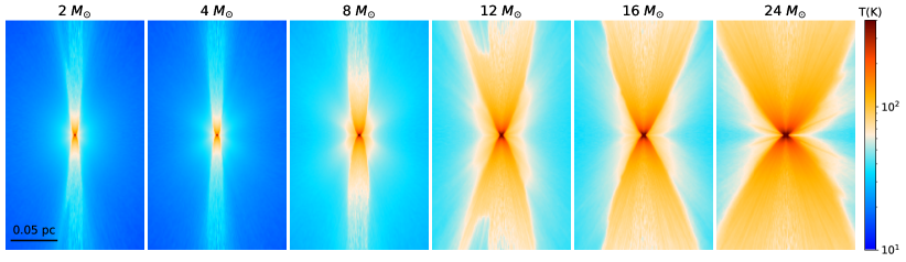
Figure 1: Temperatures of dust in a slice along the outflow axis for different protostellar masses.

2.2.2 ¹²CO, ¹³CO and C¹⁸O Emission

In order to model the line emission of multiple ¹²CO, ¹³CO, and C¹⁸O rotational transitions from the simulated outflows, we employ the publicly available radiation transfer code radmc-3d  (Dullemond et al., 2012). radmc-3d calculates level populations in accordance with the local density and temperature. The main simplifying assumptions we adopt in this modeling are that gas kinetic temperature is equal to the dust temperature, calculated above, and that the abundance of CO and its isotopologues is spatially constant. The assumption that the gas kinetic temperature is well-coupled to the dust temperature is generally expected to be the case in molecular clouds with densities $n_{\rm H}\gtrsim 10^{5}\>{\rm cm}^{-3}$, which applies to most of the regions in the simulation domain.

However, in photo-dissociation regions (PDRs) we expect there to be greater difference between dust and gas temperatures, as well as large variations in CO abundance. Full PDR modeling of the outflow structures has been carried out by Oblentseva et al. (in prep.) using a modified version of 3D-PDR (Bisbas et al. 2012). The importance of the PDR becomes greater at later evolutionary stages. The results presented in our paper should be considered the limiting cases when the PDR has only minor impact. A full comparison of our results with the PDR modeling results will be presented by Oblentseva et al. (in prep.).

We adopt a microturbulent line width of 1 km s^-1 to correspond to the typical turbulent velocity of a 60 $M_{\mathord{\odot}}$ pre-stellar core in the TCA model. Instead of performing a complete non-LTE radiative transfer calculation, radmc-3d employs an approximate Large Velocity Gradient (LVG) method (Ossenkopf, 1997) to solve the statistical equilibrium equation at each position. The density, temperature and velocity distributions used as inputs to radmc-3d  are derived from the simulation data and the dust radiative transfer calculations (see above). We assume that H₂ is the dominant collisional partner of CO, set the abundance ratios of ¹²CO/ H nuclei to a fiducial value of $10^{-4}$, and the ratio of the isotopologues ¹³CO and C¹⁸O to ¹²COto fiducial values of 62 and 500, respectively (Arce & Sargent, 2006).

3 Results

3.1 Synthetic ¹²CO, ¹³CO and C¹⁸O Maps

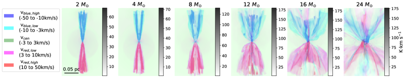
Figure 2: Synthetic ¹²CO(2-1) emission of outflows at different evolutionary stages, i.e., different protostellar mass, and viewed at an inclination angle of 58^∘to the outflow axis. Different colors indicate different velocity ranges of the integrated emission: blue-shifted high-velocity component (-50 to -10 km s^-1); blue-shifted low-velocity component (-10 to -3 km s^-1); central velocity component (-3 to 3 km s^-1); red-shifted low-velocity component (3 to 10 km s^-1); and red-shifted high-velocity component (10 to 50 km s^-1). The scalebar shows the grayscale intensity scale for each color map, and all colors in a given panel are assigned the same range of values.

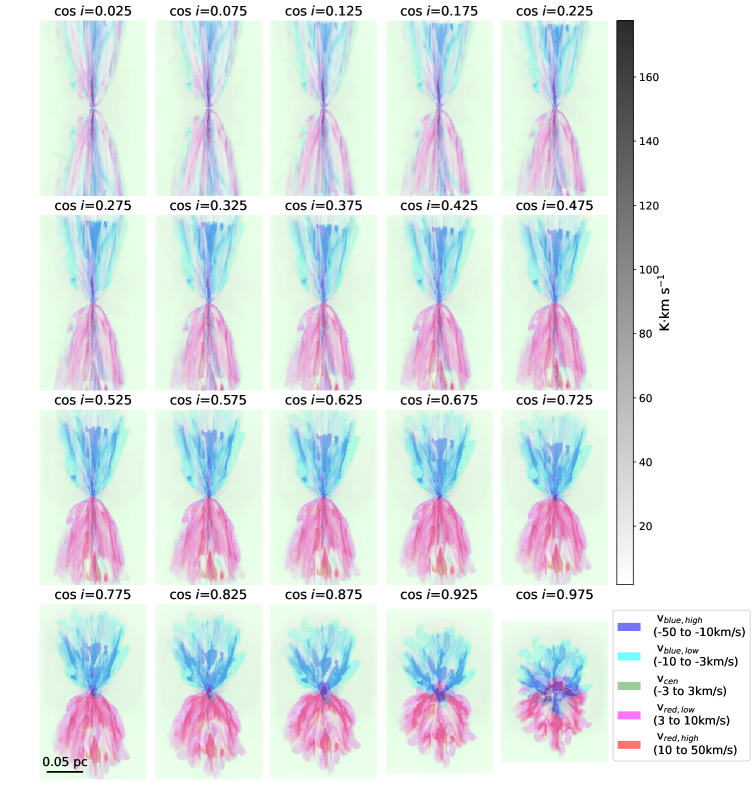
Figure 3: Synthetic ¹²CO (2-1) emission of the outflow from a 12 $M_{\mathord{\odot}}$ protostar at different inclination angles. The color description is the same as Figure 2. $\cos i=1$ corresponds to looking along the outflow (“face-on”), while $\cos i=0$ is looking across the outflow (“edge-on”).

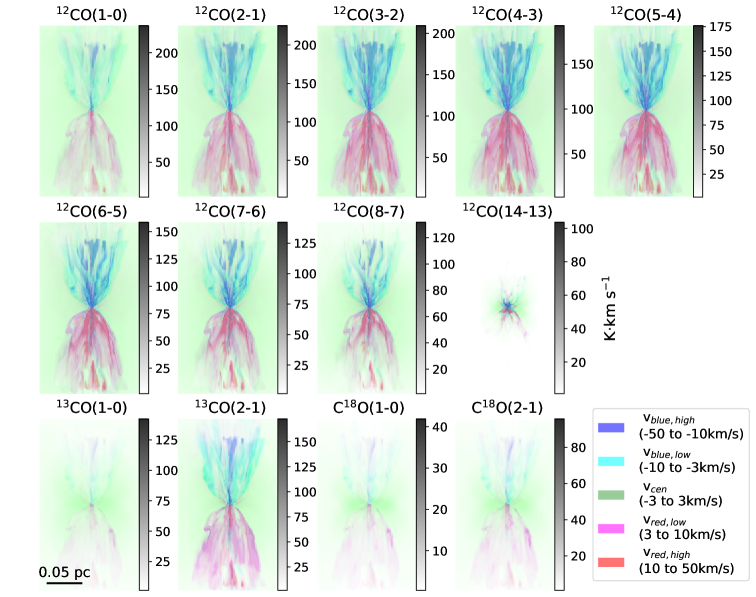
Figure 4: Synthetic emission maps for multiple transitions of ¹²CO, ¹³CO  and C¹⁸O  from a 12 $M_{\mathord{\odot}}$ star outflow at an inclination angel of 58^∘. The color description is the same as Figure 2.

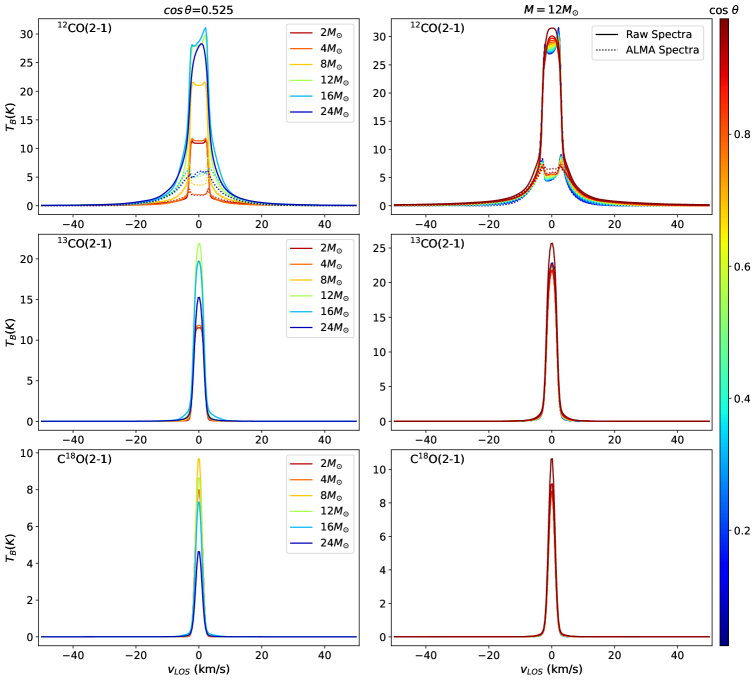
Figure 5: (a) Left column: Synthetic ¹²CO(2-1), ¹³CO(2-1), and C¹⁸O(2-1) spectra of outflows at different evolutionary stages viewed at an inclination angle of 58^∘. (b) Right column: Synthetic ¹²CO(2-1), ¹³CO(2-1), and C¹⁸O(2-1) spectra of outflows from a 12 $M_{\mathord{\odot}}$ protostellar mass viewed at different inclination angles, as labeled by the color bar. The solid lines represent the raw synthetic spectra, whereas the dotted line represents the synthetic ALMA spectra post-processed with CASA.

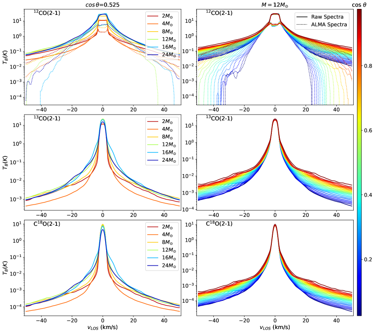
Figure 6: Similar to Figure 5, but uses a logarithmic scale.

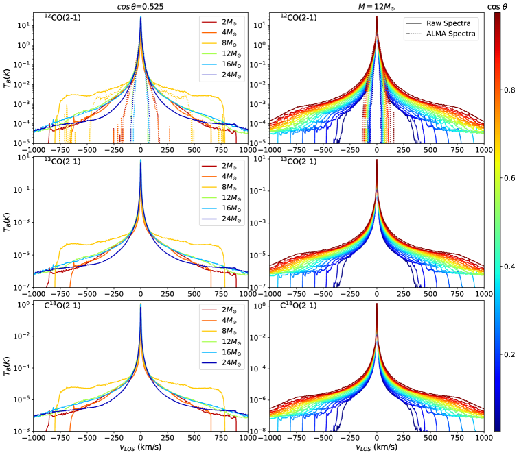
Figure 7: Similar to Figure 5, but with a broader velocity range.

We present the results of the radiative transfer calculations for 20 different inclination angles, with the cosine values of inclination angle evenly spaced between 0.025 and 0.975. This choice is the same as that used in the continuum radiative transfer model grid of Zhang & Tan (2018). Figure 2 shows the synthetic ¹²CO(2-1) emission for the outflows at different evolutionary stages, i.e., different protostellar masses, with an inclination angle of 58^∘. To facilitate the visualization of different velocity components of the outflow emission, we divide the velocity channels into five parts: the blue-shifted high-velocity component (-50 to -10 km s^-1), the blue-shifted low-velocity component (-10 to -3 km s^-1), the central velocity component (-3 to 3 km s^-1), the red-shifted low-velocity component (3 to 10 km s^-1), and the red-shifted high-velocity component (10 to 50 km s^-1). As the protostellar mass increases, the opening angle of the outflow cavity increases, as do the overall velocities in the outflow (see Staff et al., 2023). Our synthetic ¹²CO emission maps reproduce these trends.

In Figure 3, we present synthetic ¹²CO(2-1) emission of the outflow from the 12 $M_{\mathord{\odot}}$ protostar at various inclination angles. Our results indicate that, as the observed inclination angle decreases, the visible high-velocity components of the emission become more prominent and exhibit a wider-angle, more overlapping spatial distribution. This is to be expected, as the majority of the momentum in the outflow is along the outflow axis and, at lower inclinations, more and more of this velocity is along the line of sight.

In Figure 4, we present synthetic maps of multiple transitions of ¹²CO, ¹³CO and C¹⁸O, for the outflow from a 12 $M_{\mathord{\odot}}$ protostar at a fixed inclination angle of 58^∘. Note that the emission from the ground transition $J=1-0$ of ¹²CO exhibits a greater contribution from the ambient gas compared to the other ¹²CO transitions. The morphology of the outflow appears consistent across various ¹²CO transitions, except for the extreme case of the ¹²CO($J=14-13$) transition. In contrast to the other transitions, the ¹²CO(14-13) transition shows a more centralized morphology, indicating that this highly excited gas is concentrated close to the central star. This behavior can be attributed to the high kinetic temperature needed to excite ¹²CO to such high energy levels.

Figures 5a, 6a and 7a display the simulated ¹²CO(2-1), ¹³CO(2-1), and C¹⁸O(2-1) spectra of the outflows at various evolutionary stages, viewed at a fixed inclination angle of 58^∘to the outflow axis. In Figure 5a the spectra span a velocity range of -50 to 50 km s^-1, with a spectral resolution of 0.39 km s^-1, while Figure 6a shows the same information, but with a logarithmic intensity scale. As the mass of the star increases, there is a noticeable broadening of the high-velocity component. The emission at the ambient velocity of the core infall envelope also brightens as the protostellar mass increases, which is due to the warmer temperatures achieved at the later evolutionary stages. To examine the visibility of very high-velocity gas in the outflows, we present the outflow spectra with an extended velocity range of -1000 to 1000 km s^-1, with a velocity resolution of 3.9 km s^-1, in Figure 7a. Notably, when the protostellar mass exceeds 12 $M_{\mathord{\odot}}$, there is still emission present from very high-velocity gas at approximately $\pm$1000 km s^-1.

Figures 5b, 6b and 7b meanwhile show the simulated ¹²CO(2-1), ¹³CO(2-1), and C¹⁸O(2-1) spectra of the outflow from a 12 $M_{\mathord{\odot}}$ protostar at varying inclination angles. A decrease in the inclination angle also results in wider line wings, indicating an increase in the amount of high-velocity gas along the line of sight.

In Appendix A, a collection of moment maps for the synthetic outflows is displayed.

3.2 Synthetic ALMA Observations

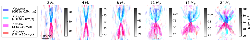
Figure 8: Same as Figure 2, but post-processed with CASA and now not displaying the ambient gas.

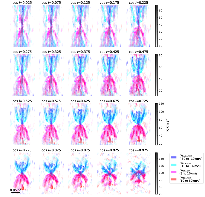
Figure 9: Same as Figure 3, but post-processed with CASA.

To replicate the type of observations made by ALMA, we utilized CASA/simalma to post-process the synthetic molecular line data of ¹²CO(2-1) generated in §3.1. Our synthetic interferometry observations were conducted using the C36-3 12-m array configuration, which was also employed in the observations described in §4. We maintained consistency by employing the same integration time of 210 seconds, and we assumed that the source was located at a distance of 2 kpc. The default value of 0.5 mm is chosen for the Precipitable Water Vapor. The resolution of the cell is set to match our simulation at 0.1 arcsec. Figure 8 illustrates the synthetic ALMA observations of ¹²CO (2-1) for outflows at different evolutionary stages, each with an inclination angle of 58^∘. The figure reveals the presence of artificial patterns resulting from the imperfect coverage in visibility space plus the CLEAN reconstruction process. It is important to note that interferometric observations typically filter out the emission from the ambient gas located at the central (or systemic) velocity, which we have omitted from the figure.

In addition, we present in Figure 9 the synthetic ALMA observations of ¹²CO (2-1) from the outflow from a 12 $M_{\mathord{\odot}}$ star at different inclination angles. As also seen in Figure 3, we observe here that the high-velocity components of the emission become increasingly prominent as the inclination angle decreases.

Figures 5, 6 and 7 display the ¹²CO(2-1) spectra of outflows at various evolutionary stages post-processed using CASA/simalma in dotted lines for the case of an inclination angle of 58^∘. These figures also show the post-processed ¹²CO(2-1) spectra of the outflow from a protostar of 12 $M_{\mathord{\odot}}$ at different inclination angles in dotted lines. Similar to the raw synthetic spectra without post-processing using CASA/simalma, we observe a broader high-velocity component in the spectra as the protostellar mass increases, and wider line wings as the inclination angle decreases. Additionally, it is important to note that the drop in emission near the central velocity is a result of missing flux due to incomplete coverage of the $uv$-plane, i.e., missing short baselines. We also see a considerable intensity drop in the high-velocity channels when compared to the raw spectra. This drop is attributed to the weak emission near the noise level at these high-velocity channels, rendering them unobservable.

3.3 Estimating the Mass, Momentum and Energy of Synthetic Outflows

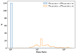
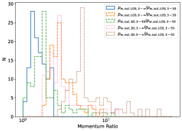
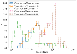
Figure 10: (a) Left: Histogram showing the ratios of outflow mass for different LOS velocity cuts. (b) Middle: Histogram showing the ratios of outflow momentum for different LOS velocity cuts and 3D velocity cuts. (c) Middle: Histogram showing the ratios of outflow energy for different LOS velocity cuts and 3D velocity cuts.

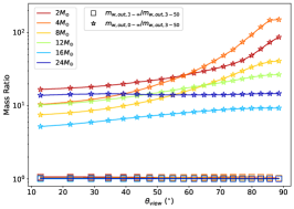
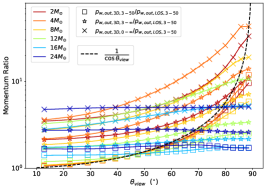
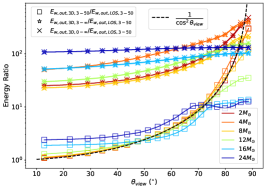
Figure 11: (a) Left: Variation of the ratios of outflow mass for different LOS velocity cuts as a function of inclination of viewing angle $\theta_{\rm view}$. (b) Middle: Variation of the ratios of outflow momentum for different LOS velocity cuts as a function of inclination of viewing angle $\theta_{\rm view}$. (c) Middle: Variation of the ratios of outflow energy for different LOS velocity cuts as a function of inclination of viewing angle $\theta_{\rm view}$.

In this section, we assess the estimation of outflow mass, momentum and energy derived from synthetic molecular line emission and compare it with the true values obtained from simulations. First, we investigate the impact of a line-of-sight (LOS) velocity cut on the estimation of outflow mass, momentum, and energy. We perform this analysis using only the simulation data without incorporating synthetic observations. In the simulations, the outflow gas can be defined as the gas moving outward from the central source above some given velocity threshold. In real observations, it can be difficult to distinguish between the ambient gas and the outflow gas when the LOS velocity is close to the turbulent velocity of the cloud. In addition, it can be challenging to cover the entire velocity range of the outflow in the spectra with enough signal to noise to measure the highest velocity components. To address these issues, we apply LOS velocity cuts as masks on the outflow gas and define the observed outflow mass as $m_{\rm w,out,LOS,3-50}$, representing the mass of outflowing gas with an absolute LOS velocity between 3 and 50 km s^-1. We also define $m_{\rm w,out,LOS,3-\infty}$ as the outflow mass with an absolute LOS velocity over 3 km s^-1, which helps quantify the missing mass at $v_{\rm LOS}>50$ km s^-1. Furthermore, we define the total outflow mass, denoted as $m_{\rm w,out,LOS,0-\infty}$, which encompasses the outflow gas covering the entire velocity range. The ratio $\rm m_{\rm w,out,LOS,0-\infty}/m_{\rm w,out,LOS,3-50}$ provides insights into the missing mass near the rest frame velocity at $v_{\rm LOS}<3$ km s^-1 and at $v_{\rm LOS}>50$ km s^-1.

Figure 10a presents the distribution of $m_{\rm w,out,LOS,3-\infty}/m_{\rm w,out,LOS,3-50}$ and $m_{\rm w,out,LOS,0-\infty}/m_{\rm w,out,LOS,3-50}$. Table 1 displays the statistical values for these ratios. It is evident that the outflow gas mass with LOS velocities exceeding 50 km s^-1 is negligible compared to the mass with LOS velocities ranging from 3 to 50 km s^-1. However, there is a substantial amount of mass, approximately a factor of 10 or more, that is being overlooked near the rest frame velocity ($v_{\rm LOS}<3$ km s^-1).

We then establish the definition for observed outflow LOS momentum, denoted as $p_{\rm w,out,LOS,3-50}$, which encompasses outflow gas with an absolute LOS velocity ranging from 3 to 50 km s^-1. Additionally, $p_{\rm w,out,LOS,3-\infty}$ is defined as the outflow LOS momentum derived from gas with an absolute LOS velocity over 3 km s^-1, while $p_{\rm w,out,LOS,0-\infty}$ represents the total outflow LOS momentum. Considering that outflowing gas moves in 3D space and not solely along the LOS direction, we also define the outflow 3D momentum, denoted as $p_{\rm w,out,3D,3-50}$, $p_{\rm w,out,3D,3-\infty}$, and $p_{\rm w,out,3D,0-\infty}$, representing the outflow 3D momentum with different LOS velocity cutoffs. Analogously, we define the outflow LOS energy and outflow 3D energy.

Figure 10b illustrates the distribution of outflow momentum ratios. The ratio $p_{\rm w,out,LOS,3-\infty}/p_{\rm w,out,LOS,3-50}$ denotes the missing outflow LOS momentum due to the high-velocity cutoff ($v_{\rm LOS}>50$ km s^-1). On the other hand, $p_{\rm w,out,LOS,0-\infty}/p_{\rm w,out,LOS,3-50}$ indicates the missing outflow LOS momentum from the gas near the rest frame velocity ($v_{\rm LOS}<3$ km s^-1) and at high velocities ($v_{\rm LOS}>50$ km s^-1). Additionally, $p_{\rm w,out,3D,3-50}/p_{\rm w,out,LOS,3-50}$ signifies the conversion factor between the outflow 3D momentum and the 1D LOS momentum for the observed outflow gas with an absolute velocities from 3 and 50 km s^-1. Finally, $p_{\rm w,out,3D,0-\infty}/p_{\rm w,out,LOS,3-50}$ represents the total conversion factor between the outflow total 3D momentum and the observed 1D LOS momentum. We observed that the high-velocity gas with $v_{\rm LOS}>50$ km s^-1, while having almost negligible outflow mass, carries a noticeable amount of momentum due to its high velocity. Conversely, the gas near the rest frame velocity ($v_{\rm LOS}<3$ km s^-1), which accounts for a factor of ten or more in mass compared to the observed mass, contributes to the momentum by only a factor of 2. Overall, when estimating the total 3D momentum from the LOS momentum with an absolute LOS velocity ranging from 3 to 50 km s^-1, there is a likely underestimation of the total 3D momentum by a factor of 4 and up to 40.

Figure 10c displays the distribution of outflow energy ratios. Notably, the high-velocity gas with $v_{\rm LOS}>50$ km s^-1 carries a significant amount of energy, while the gas near the rest frame velocity ($v_{\rm LOS}<3$ km s^-1) contributes negligible outflow energy. In general, when estimating the total 3D energy from the LOS energy with an absolute LOS velocity ranging from 3 to 50 km s^-1, there is a likely underestimation of the total 3D energy by a factor of 50 and up to 500. We present the statistical values for all the ratios discussed above in Table 1.

Table 1: Table of mass, momentum and energy ratios for different LOS velocity cuts

Ratios	Mean	Median	Min	Max	Std
$m_{\rm w,out,LOS,3-\infty}/m_{\rm w,out,LOS,3-50}$	1.025	1.020	1.003	1.072	0.019
$m_{\rm w,out,LOS,0-\infty}/m_{\rm w,out,LOS,3-50}$	23.68	14.71	5.207	150.5	24.33
$p_{\rm w,out,LOS,3-\infty}/p_{\rm w,out,LOS,3-50}$	1.563	1.473	1.085	2.308	0.340
$p_{\rm w,out,LOS,0-\infty}/p_{\rm w,out,LOS,3-50}$	3.151	2.790	1.781	8.766	1.323
$p_{\rm w,out,3D,3-50}/p_{\rm w,out,LOS,3-50}$	2.270	1.725	1.060	11.90	1.712
$p_{\rm w,out,3D,3-\infty}/p_{\rm w,out,LOS,3-50}$	3.506	2.744	1.703	13.99	2.320
$p_{\rm w,out,3D,0-\infty}/p_{\rm w,out,LOS,3-50}$	7.892	5.055	2.763	43.29	7.265
$E_{\rm w,out,LOS,3-\infty}/E_{\rm w,out,LOS,3-50}$	21.23	16.50	2.375	92.08	17.44
$E_{\rm w,out,LOS,0-\infty}/E_{\rm w,out,LOS,3-50}$	21.38	16.66	2.748	92.15	17.40
$E_{\rm w,out,3D,3-50}/E_{\rm w,out,LOS,3-50}$	17.63	3.945	1.088	301.0	44.22
$E_{\rm w,out,3D,3-\infty}/E_{\rm w,out,LOS,3-50}$	98.82	83.54	22.64	439.3	72.24
$E_{\rm w,out,3D,0-\infty}/E_{\rm w,out,LOS,3-50}$	101.5	85.24	22.76	480.3	77.30

We then investigate how the viewing angle $\theta_{\rm view}$ affects the previously studied ratios. Figure 11 illustrates the variation of the ratios of outflow mass, momentum, and energy for different LOS velocity cuts as a function of the viewing angle $\theta_{\rm view}$. As $\theta_{\rm view}$ increases, there is an increase in the amount of missed mass, momentum, and energy, primarily caused by most of the outflowing gas moving perpendicular to the LOS, making them unobservable in spectra with a LOS velocity between 3 and 50 km s^-1. It is important to highlight that the cases involving 16 $M_{\mathord{\odot}}$ and 24 $M_{\mathord{\odot}}$ stars exhibit a more flattened trend in the ratios with respect to $\theta_{\rm view}$. This behavior can be attributed to the larger opening angle in these cases compared to the lower mass ones. As a result, the velocity distribution becomes more isotropic, with multiple launching directions rather than a single dominant one. By analyzing Figure 11, we can derive correction factors to adjust the true 3D values based on the observed 1D LOS values for different outflows with various inclination angles and evolutionary stages.

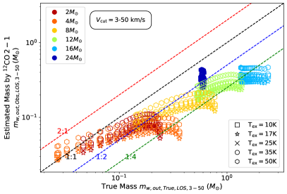
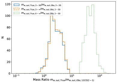
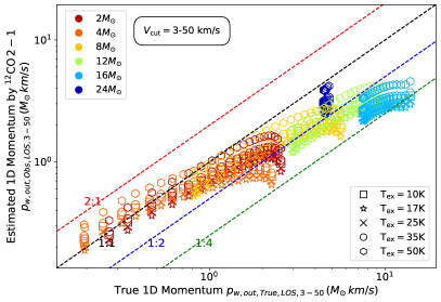
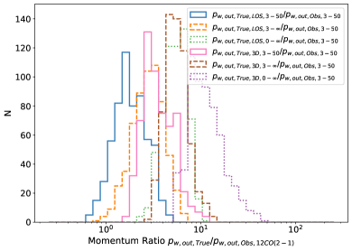
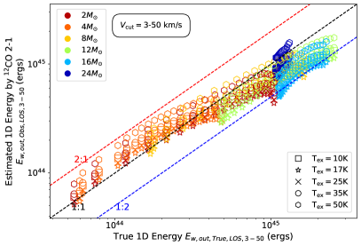
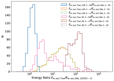
Figure 12: Left column: Comparison of the mass ($1^{st}$ row), momentum ($2^{nd}$ row) and energy ($3^{rd}$ row) estimates obtained for different inclination angles using ¹²CO(2-1) with a LOS velocity cutoff between 3 to 50 km s^-1, and the corresponding true outflow values with the same velocity cutoff. Right column: the ratios between ¹²CO(2-1) calculated mass ($1^{st}$ row), momentum ($2^{nd}$ row) and energy ($3^{rd}$ row) and the true simulation-derived values for different LOS velocity cuts.

We next determine the outflow mass, momentum and energy from the raw synthetic molecular spectra and compared it to the true outflow values obtained from simulations. To ensure a fair comparison, only the mass, momentum and energy with a LOS velocity above a certain threshold were considered in the true outflow values. This means that to obtain the total outflow mass momentum and energy, we must account for the missing fraction as previously mentioned. Our primary goal in this study is to assess the uncertainty in estimating outflow mass momentum and energy from molecular spectra.

The column density of CO molecules that are in the upper level of a transition from level $u\rightarrow l$ can be expressed as

$$N_{u,\rm CO}=\frac{8\pi k\nu^{2}}{hc^{3}A_{ul}}\int T_{b}(V)dV$$ (1)

where $k$ is Boltzmann’s constant, $\nu$ is the frequency of the transition from level $u\rightarrow l$, $h$ is Planck’s constant, $c$ is the speed of light, $A_{ul}$ is the spontaneous decay rate from upper level $u$ to lower level $l$, and $T_{b}$ is the brightness temperature. The total CO column density $N_{\rm tot}$ is related to the upper level column density $N_{u}$ through

$$N_{\rm tot,CO}=f_{u}f_{b}N_{u,\rm CO}.$$ (2)

In the equation above, the level correction factor $f_{u}$ can be determined analytically under the assumption of local thermodynamic equilibrium (LTE) as

$$f_{u}=\frac{Q(T_{\rm ex})}{g_{u}\exp\left(-\frac{h\nu}{kT_{\rm ex}}\right)}$$ (3)

where $g_{u}$ is the statistical weight of the upper-level. $T_{\rm ex}$ is the excitation temperature and $Q(T_{\rm ex})=kT_{\rm ex}/hB_{0}$ is the LTE partition function, with $B_{0}$ being the rotational constant. The correction for the background is given by

$$f_{b}=\left[1-\frac{e^{\frac{h\nu}{kT_{\rm ex}}}-1}{e^{\frac{h\nu}{kT_{\rm bg}}}-1}\right]^{-1}$$ (4)

where $T_{\rm bg}$ is the background temperature, assumed to be 2.7K. The final mass is calculated as follows:

$$m_{\rm tot}=\sum_{i}\mu m_{\rm H}d^{2}\frac{N_{\rm tot,CO}}{X_{\rm CO-H}},$$ (5)

where $\mu=1.4$ takes into account the mass of helium per H-nucleus, $m_{\rm H}$ is the mass of an H-nucleus, $d$ represents the physical scale of each pixel in the map, $X_{\rm CO-H}$ is the abundance ratio between CO and H-nuclei, and $\sum_{i}$ indicates the summation over all pixels.

The 1D LOS momentum and energy of outflows are calculated using the following equations:

$$p=\sum_{i,j,k}{X_{\rm CO-H}}m_{{\rm CO},i,j,k}|v_{i,j,k}-\overline{v_{\rm c}}|,$$ (6)

$$E=\sum_{i,j,k}\frac{1}{2}{X_{\rm CO-H}}m_{{\rm CO},i,j,k}(v_{i,j,k}-\overline{v_{\rm c}})^{2},$$ (7)

where $m_{{\rm CO},i,j,k}$ represents the mass of CO in the $(i,j,k)$ grid cell in the position-position-velocity (ppv) cube, $X_{\rm CO-H}$ is the abundance ratio between CO and H-nuclei, $v_{i,j,k}$ represents the LOS velocity of the CO in that grid cell, and $\overline{v_{\rm c}}$ is the global central LOS velocity of the outflow.

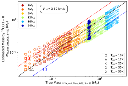
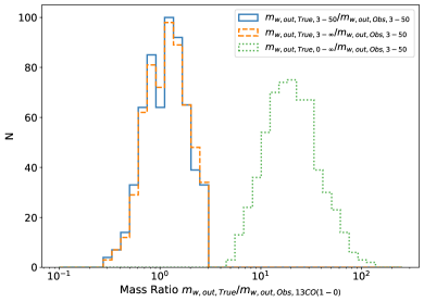
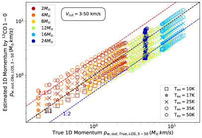
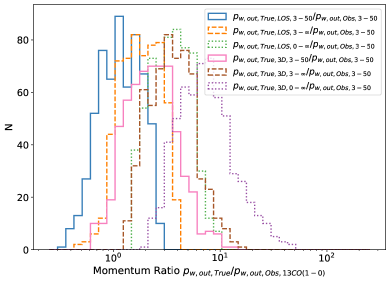
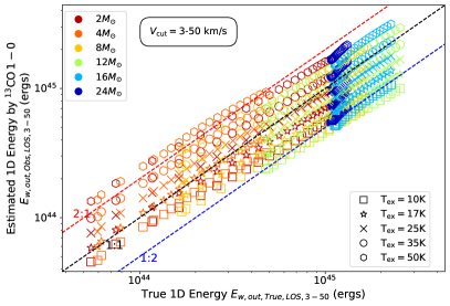
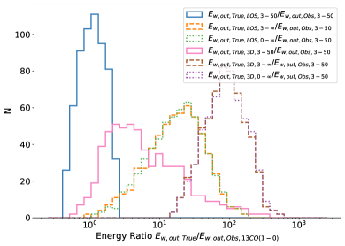
Figure 13: Left column: Comparison of the mass ($1^{st}$ row), momentum ($2^{nd}$ row) and energy ($3^{rd}$ row) estimates obtained for different inclination angles using ¹³CO(1-0) with a LOS velocity cutoff between 3 to 50 km s^-1, and the corresponding true outflow values with the same velocity cutoff. Right column: the ratios between ¹³CO(1-0) calculated mass ($1^{st}$ row), momentum ($2^{nd}$ row) and energy ($3^{rd}$ row) and the true simulation-derived values for different LOS velocity cuts.

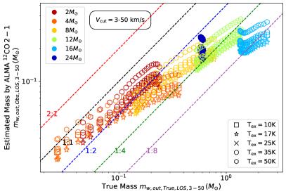
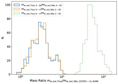
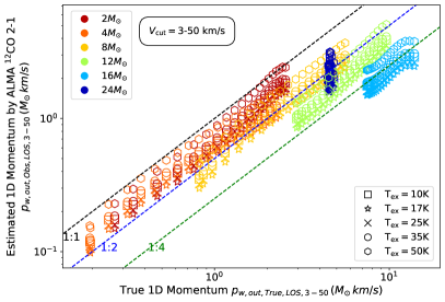
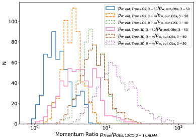
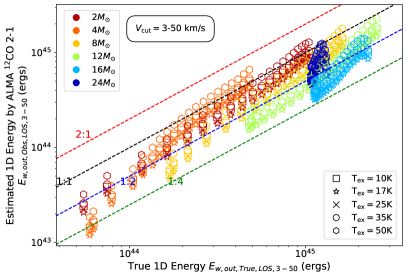
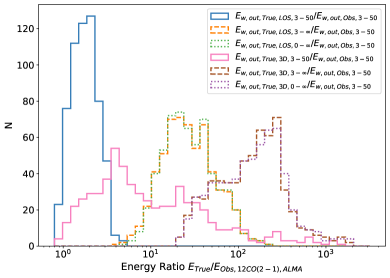
Figure 14: Left column: Comparison of the mass ($1^{st}$ row), momentum ($2^{nd}$ row) and energy ($3^{rd}$ row) estimates obtained for different inclination angles using synthetic ALMA ¹²CO(2-1) post-processed with CASA/simalma with a LOS velocity cutoff between 3 to 50 km s^-1, and the corresponding true outflow values with the same velocity cutoff. Right column: the ratios between synthetic ALMA ¹²CO(2-1) calculated mass ($1^{st}$ row), momentum ($2^{nd}$ row) and energy ($3^{rd}$ row) and the true simulation-derived values for different LOS velocity cuts.

We determine the mass of the outflow using ¹²CO(2-1) and ¹³CO(1-0) lines separately. Since it is not possible to determine the excitation temperature based on a single molecular line observation, certain assumptions must be made regarding the excitation temperature. We consider multiple excitation temperatures for the outflow gas, ranging from 10 K to 50 K. Our analysis reveals that assuming an excitation temperature of 17 K for ¹²CO(2-1) leads to the lowest estimation of the outflow mass. On the other hand, when using ¹³CO(1-0), the estimated mass of the outflow increases as the excitation temperature increases.

Figure 12 presents a comparison between the true outflow mass, momentum, and energy and the corresponding estimated values obtained from ¹²CO(2-1) lines. The estimation is carried out using a LOS velocity cutoff between 3 and 50 km s^-1. The choice of 3 km s^-1 as the lower cutoff mainly excludes the ambient gas, which exhibits a turbulent velocity of approximately 1 km s^-1. On the other hand, the upper cutoff of 50 km s^-1 is selected since most outflow observations cover the velocity range up to 50 km s^-1, and beyond this limit, the outflow gas emission becomes too faint to be detected, as evident from the spectra of the three sources in §4. The estimated outflow mass and momentum using ¹²CO(2-1) spectra show a scatter within a factor of 4 compared to the true values. However, for higher outflow mass and momentum, there is a noticeable underestimation. This suggests that ¹²CO(2-1) may be optically thick for certain outflow gas, leading to the trapping of emission and resulting in lower measured mass values. In contrast, the estimated outflow energy using ¹²CO(2-1) spectra demonstrates a scatter within a factor of 2 compared to the true values. This indicates that the relatively low-velocity gas is likely to be optically thick, while the high-velocity gas is optically thin. The optically thin high-velocity gas significantly contributes to the outflow energy. Figure 12 also presents the distribution of outflow mass, momentum, and energy ratios between the true values and the observed values from ¹²CO(2-1). Notably, the outflow gas at high-velocity channels ($v_{\rm LOS}>50$ km s^-1) contributes negligible mass but significant momentum and energy. In summary, the true outflow mass is underestimated by approximately a factor of 50 when compared to the mass calculated from ¹²CO(2-1) spectra with a LOS velocity between 3 and 50 km s^-1. The true 3D outflow momentum is approximately 10 times larger than the LOS momentum calculated from ¹²CO(2-1) spectra with the same velocity cutoff. The true 3D outflow energy is approximately 150 times larger than the LOS energy calculated from ¹²CO(2-1) spectra with a LOS velocity between 3 and 50 km s^-1.

Figure 13 presents a comparison between the true outflow mass, momentum, and energy and the corresponding estimated values obtained from ¹³CO(1-0) lines. The estimated outflow mass, momentum and energy using ¹³CO(1-0) spectra show a scatter within a factor of 2 compared to the true values. And there is no significant underestimation when the outflow mass is high, which implies that ¹³CO(1-0) is more optically thin compared to ¹²CO(2-1). In addition we find that an assumption between 17 to 35 K is likely sufficient for accurately deriving the outflow mass, momentum and energy from ¹³CO(1-0) spectra. Figure 13 also presents the distribution of outflow mass, momentum, and energy ratios between the true values and the observed values from ¹³CO(1-0). In summary, the true outflow mass is underestimated by approximately a factor of 20 when compared to the mass calculated from ¹³CO(1-0) spectra with a LOS velocity between 3 and 50 km s^-1. The true 3D outflow momentum is approximately 7 times larger than the LOS momentum calculated from ¹³CO(1-0) spectra with the same velocity cutoff. The true 3D outflow energy is approximately 100 times larger than the LOS energy calculated from ¹³CO(1-0) spectra with a LOS velocity between 3 and 50 km s^-1.

In Figure 14, we compare the true outflow mass, momentum, and energy with the corresponding estimated values obtained from synthetic ALMA ¹²CO(2-1) observations generated in §3.2. The estimated outflow mass using synthetic ALMA ¹²CO(2-1) spectra shows a scatter within a factor of 8 compared to the true values. Likewise, the estimated outflow momentum and energy using synthetic ALMA ¹²CO(2-1) spectra show a scatter within a factor of 4 compared to the true values. However, it is worth noting that there is a systematic underestimation of mass, momentum, and energy when using synthetic ALMA ¹²CO(2-1) spectra compared to the raw ¹²CO(2-1) spectra in Figure 12. This discrepancy is likely due to the interferometry missing flux of the gas with a LOS velocity between 3 and 50 km s^-1, especially near 3 km s^-1. Figure 14 also presents the distribution of outflow mass, momentum, and energy ratios between the true values and the observed values from synthetic ALMA ¹²CO(2-1) spectra. In summary, the true outflow mass is underestimated by approximately a factor of 50 when compared to the mass calculated from synthetic ALMA ¹²CO(2-1) spectra with a LOS velocity between 3 and 50 km s^-1. The true 3D outflow momentum is approximately 15 times larger than the LOS momentum calculated from synthetic ALMA ¹²CO(2-1) spectra with the same velocity cutoff. The true 3D outflow energy is approximately 250 times larger than the LOS energy calculated from synthetic ALMA ¹²CO(2-1) spectra with a LOS velocity between 3 and 50 km s^-1.

Furthermore, we provide mass, momentum and energy estimates for synthetic outflows utilizing the ¹²CO(1-0) line emission and assess their precision compared to the true values attained from simulations in Appendix B.

3.4 Estimating the Mass Outflow Rate and Momentum Outflow Rate

In this section, we assess the mass outflow rate and momentum outflow rate using synthetic ALMA ¹²CO(2-1) data. Initially, we quantify the true values of these rates by calculating the mass and momentum flux across a plane at specific heights from the central stars, as obtained from simulations. The mass and momentum flux are measured at a height of 25,000 au, i.e., at the top of the simulation domain. Table 2 presents a summary of the mass outflow rates and momentum outflow rates, measured at 25,000 AU, along with the injection rates of the primary outflow reported in Staff et al. (2023). Note that the mass outflow rate includes entrained gas, i.e., primary outflow gas launched directly by the disk wind plus swept-up secondary outflow material. As emphasized in Staff et al. (2023), the entrained gas can be up to nine times larger than the directly injected mass from the central source. On the other hand, due to the conservation of momentum, the momentum outflow rate is a more direct tracer of the input disk wind properties, i.e., momentum injection rate of the primary outflow.

Table 2: Summary of mass outflow rate and momentum outflow rate^a

$m_{*}$	$h_{\rm max}$	$\dot{m}_{\rm w,out}$	$\dot{m}_{\rm w,inj}$	$\dot{p}_{\rm w,out}$	$\dot{p}_{\rm w,inj}$	$\dot{m}_{\rm w,out}/\dot{m}_{\rm w,inj}$	$\dot{p}_{\rm w,out}/\dot{p}_{\rm w,inj}$
($M_{\odot}$)	($10^{3}\>$AU)	($10^{-5}\,M_{\odot}{\rm yr}^{-1}$)	($10^{-5}\,M_{\odot}{\rm yr}^{-1}$)	($10^{-3}\,M_{\odot}{\rm km\,s^{-1}\,yr}^{-1}$)	($10^{-3}\,M_{\odot}{\rm km\,s^{-1}\,yr}^{-1}$)
2	25.0	6.9	1.4	10.5	9.9	4.98	1.06
4	25.0	2.9	2	8.8	9.4	1.5	0.94
8	25.0	3.2	2.7	12.4	14.2	1.2	0.87
12	25.0	11.0	-	27.4	-	-	-
16	25.0	13.0	3.2	45.0	41.2	4.1	1.09
24	25.0	19.6	3.3	55.3	49.5	5.9	1.12
Notes:
a Outflow mass injection rate ($\dot{m}_{\rm w,inj}$) and outflow momentum injection rate ($\dot{p}_{\rm w,inj}$) are reported in Staff et al. (2023). The mass outflow rate ($\dot{m}_{\rm w,out}$) and momentum outflow rate ($\dot{p}_{\rm w,out}$) are measured at the maximum height in the simulation domain that captures the entire outflow moving across a surface in the $z$ direction (reported in the second column).

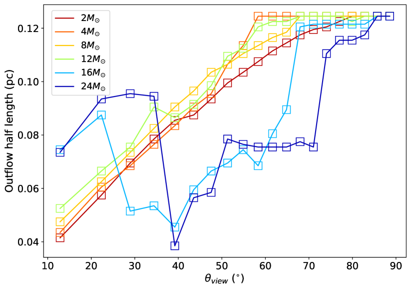
Figure 15: Variation of the outflow length (half-length, i.e., one side) as a function of inclination of viewing angle $\theta_{\rm view}$.

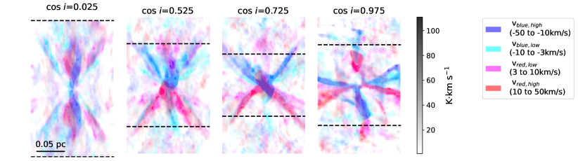
Figure 16: Synthetic ALMA ¹²CO(2-1) emission of the outflow from a 24 $M_{\mathord{\odot}}$ protostar at different inclination angles. The black dashed lines represent the boundaries of the outflow length. The color description is the same as Figure 2.

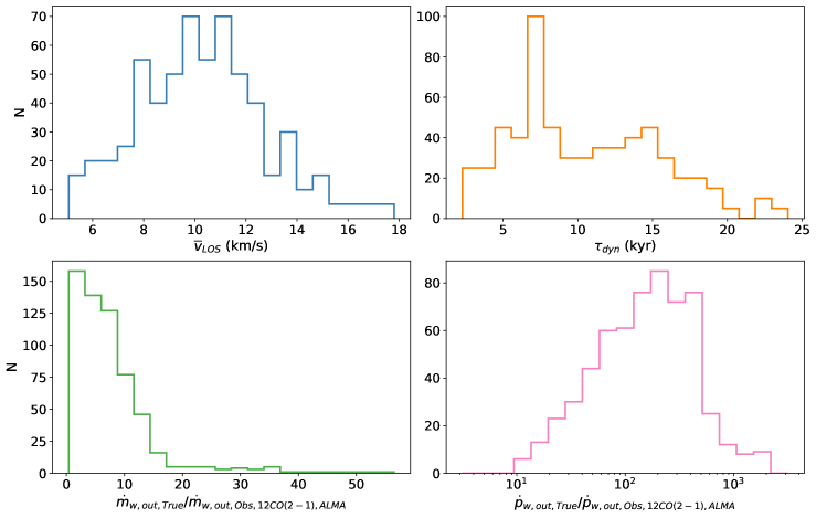
Figure 17: Upper left: Histogram depicting the mass-weighted mean LOS velocity of the outflow. Upper right: Histogram showing the outflow dynamic timescale. Lower left: Histogram displaying the ratio between the true mass outflow rate and the observed mass outflow rate. Lower right: Histogram presenting the ratio between the true momentum outflow rate and the observed momentum outflow rate.

To estimate the mass outflow rate and momentum outflow rate from synthetic ALMA ¹²CO(2-1) data, we adopt a similar observational approach as in Zhang et al. (2019a). We first determine the outflow length based on the integrated intensity of the synthetic ALMA ¹²CO(2-1) data, considering only emission above 3$\sigma$ as valid. Using a box to enclose the outflow emission, we obtain the length of the box, representing the outflow length derived from synthetic ALMA ¹²CO(2-1) data. Figure 15 displays the variation of the outflow length (considering one sided lobe of the outflow, i.e., a half-length) as a function of the inclination angle $\theta_{\rm view}$. We observe that for protostellar masses between 2 $M_{\mathord{\odot}}$ and 12 $M_{\mathord{\odot}}$, the outflow length increases with $\theta_{\rm view}$. However, we observe a non-uniform trend for the 16 $M_{\mathord{\odot}}$ and 24 $M_{\mathord{\odot}}$ cases, likely due to the large opening angle of the outflow, where the cavity wall is distinct, but the emission inside the cavity remains unobserved. An example of this behavior for the 24 $M_{\mathord{\odot}}$ case at several different viewing angles is shown in Figure 16.

Next, we compute the mass-weighted mean LOS velocity of the outflow using the formula:

$$\overline{v}_{\rm LOS}=p_{\rm w,out,obs,12CO(2-1),ALMA}/m_{\rm w,out,obs,12CO(2-1),ALMA},$$ (8)

where $m_{\rm w,out,obs,12CO(2-1),ALMA}$ represents the observed outflow mass, and $p_{\rm w,out,obs,12CO(2-1),ALMA}$ is the observed 1D LOS momentum. Furthermore, we estimate the dynamical timescale $\tau_{\rm dyn}$ of the outflow by calculating the ratio between the half length of the outflow and the mass-weighted mean LOS velocity. Consequently, we can determine the observed mass outflow rate and momentum outflow rate by dividing $m_{\rm w,out,obs,12CO(2-1),ALMA}$ by $\tau_{\rm dyn}$ and $p_{\rm w,out,obs,12CO(2-1),ALMA}$ by $\tau_{\rm dyn}$, respectively.

Figure 17 illustrates the distribution of the mass-weighted mean LOS velocity and the dynamical timescale of outflows, estimated from synthetic ALMA ¹²CO(2-1) data. The average mass-weighted mean LOS velocity is approximately 10 km s^-1, which is slightly lower than the observational estimate of 13 km s^-1 reported in Zhang et al. (2019a) for G339.88. Additionally, the typical dynamical timescale of the outflows is around 7 kyr, which is shorter than the value of 12 kyr reported in Zhang et al. (2019a). It is important to consider that the dynamical timescale of the outflows can be sensitive to the chosen length of the outflow. In our study, our half domain is limited to 25,000 AU, which represents the lower limit of typical outflows. This choice results in a notably shorter dynamical timescale of the outflows.

Figure 17 also displays the distribution of the ratio between the true mass outflow rate and the observed estimate of the mass outflow rate from ¹²CO(2-1). Similarly, the figure also shows the ratio between the true momentum outflow rate and the observed estimate of the momentum outflow rate from¹²CO(2-1). In general, the true mass outflow rate is about 7 times larger (but with wide variation in this factor, i.e., depending on viewing angle and $m_{*}$) than the observed mass outflow rate calculated from synthetic ALMA ¹²CO(2-1) data. Similarly, the true momentum outflow rate is about 200 times larger (but with wide variation in this factor, i.e., depending on viewing angle and $m_{*}$) than the observed momentum outflow rate calculated from synthetic ALMA ¹²CO(2-1) data.

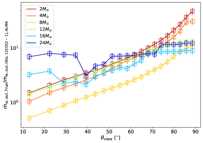
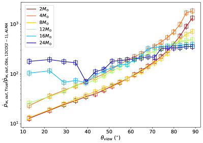
Figure 18: Left (a): Variation of the ratio between the true mass outflow rate and the observed mass outflow rate as a function of inclination of viewing angle $\theta_{\rm view}$. Right (b): Variation of the ratio between the true momentum outflow rate and the observed momentum outflow rate as a function of inclination of viewing angle $\theta_{\rm view}$. The error bars represent the standard deviation of the ratio obtained using different assumptions of excitation temperatures.

Figure 18a demonstrates the impact of the viewing angle and protostellar mass on the ratio between the true mass outflow rate and the observed mass outflow rate. As the viewing angle increases, there is a significant rise in this ratio. This ratio remains relatively stable in the case of a 24 $M_{\mathord{\odot}}$ protostellar mass, which possesses a wider opening angle, making it less influenced by the viewing angle. For relatively early evolutionary stages, i.e., $m_{*}\lesssim 12\>M_{\odot}$, there is a relatively tight relation between the mass flux correction factor and viewing angle, with a typical intermediate value of $\sim 10$. Figure 18b demonstrates a similar trend for the ratio between the true momentum outflow rate and the observed momentum outflow rate. Like the mass outflow rate, this ratio increases with the viewing angle, with relatively simple monotonic behavior for $m_{*}\lesssim 12\>M_{\odot}$. For typical viewing angles, i.e., $\sim 60^{\circ}$, the momentum flux correction factor is $\sim 100$.

4 Comparison to ALMA Observations of Outflows

4.1 Overview of CO Morphologies of G35.30, G45.47 and G338.88

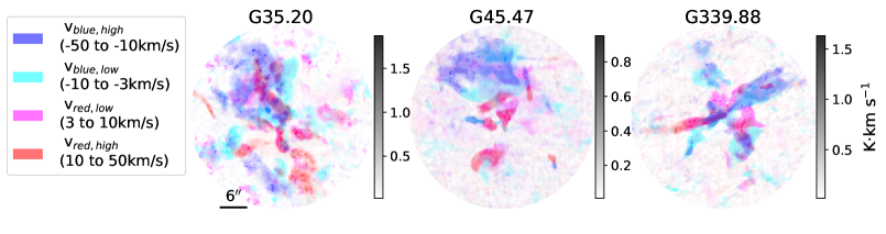
Figure 19: ¹²CO(2-1) emission of three observed outflows G35.20 (Zhang et al., 2022), G45.47 (Zhang et al., 2019b), and G339.88 (Zhang et al., 2019a). The color description is the same as Figure 8.

In order to compare the simulated CO emissions with observational data, we show ¹²CO(2-1) emission maps of outflows from three massive protostellar objects, G35.20$-$0.74N (hereafter G35.20; Sánchez-Monge et al. 2013; Zhang et al. 2022), G45.47+0.05 (hereafter G45.47; Zhang et al. 2019b), and G339.88$-$1.26 (hereafter G339.88; Zhang et al. 2019a). The distances to G35.20, G45.47, and G339.88 are 2.2 kpc, 8.4 kpc, and 2.1 kpc, respectively.

The presented ¹²CO(2-1) data were obtained with ALMA in the C36-3 configurations on September 8 (G35.20), April 24 (G45.47), and April 4 (G339.88) of 2016 (ALMA project ID: 2015.1.01454.S) with baselines ranging from 15 m to 463 m. The integration time for each source was 3.5 min. The ¹²CO(2-1) data of G35.20 and G339.88 were previously presented by Zhang et al. (2022, 2019a), and the continuum data of G45.47 obtained in the same observation were presented by Zhang et al. (2019b). We refer the reader to these papers for more details of the observations.

The ¹²CO(2-1) data were calibrated and imaged in CASA. After pipeline calibration, self-calibration using the continuum data was performed and applied to the CO line data. The CASA tclean task was used to image the data, using Briggs weighting with the robust parameter set to 0.5. For G35.20, G45.47, and G339.88, the synthetic beams of the ¹²CO images are Gaussian with a size of 0.″25. Figure 19 shows the integrated ¹²CO emissions of these sources in a similar way as the simulated emission maps presented above.

4.2 Comparison of Observational and Synthetic Outflow ¹²CO (2-1) Spectra

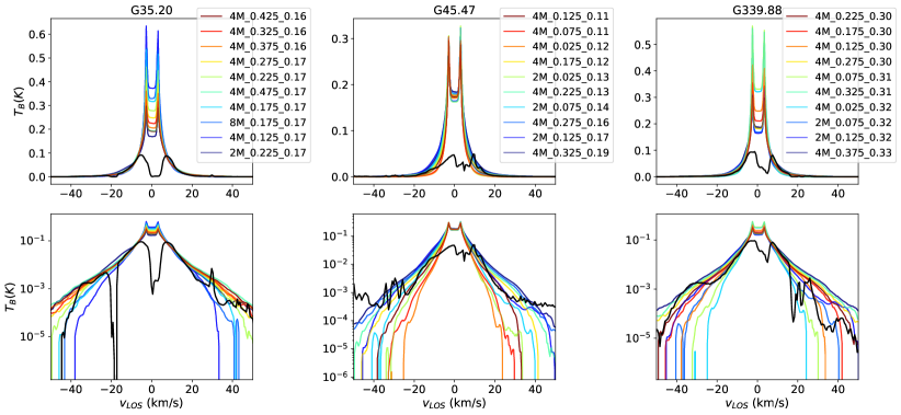
Figure 20: Fitting between the observed ¹²CO (2-1) outflows and the synthetic ALMA ¹²CO (2-1) spectra post-processed with CASA/simalma. The observed outflow ¹²CO (2-1) spectra are depicted using black lines. The legends present the top ten best fitting results, where the first number corresponds to the protostellar mass, the middle number represents the cosine value of the inclination angle, and the last number denotes the $\chi^{2}$ value.

In this section, we conduct $\chi^{2}$ fittings of the observed outflow ¹²CO(2-1) spectra with our synthetic ALMA ¹²CO(2-1) spectra. To avoid the missing flux issue near the central velocity, we restrict our fitting to spectra with an absolute LOS velocity exceeding 6 km s^-1. Additionally, since accurately determining the central velocity is challenging, we introduce a free parameter $v_{\rm offset}$ to the fitting process. This parameter is restricted to within $\pm$6 km/s. Another free parameter $f_{\rm scale}$ is used to set the emission scale of the synthetic spectrum. Thus, we only have two free parameters in the $\chi^{2}$ fitting process for each protostellar mass and inclination angle. We obtain the minimum $\chi^{2}$ for each protostellar mass and inclination angle and subsequently arrange the $\chi^{2}$ values to identify the best-fitting parameters. The results of fitting the observed outflows and our synthetic spectra are presented in Figure 20. The ten best fitting results, along with their respective $\chi^{2}$ values, are listed in the figure legend. It is important to mention that the initial core mass in the simulation is fixed at 60 $M_{\mathord{\odot}}$, while in reality, initial core masses may vary. In order to ensure a fair comparison, we employ the ratio between the protostellar mass and the initial core mass, denoted as $m_{*}/M_{c}$, as a criterion to compare our fitting outcomes with those obtained from spectral energy distribution (SED) fitting results presented in Fedriani et al. (2023).

Our fitting analysis suggests that the protostellar mass of G35.20 likely falls within the range of 2 $M_{\mathord{\odot}}$ to 8 $M_{\mathord{\odot}}$, corresponding to a $m_{*}/M_{c}$ ratio between 0.033 and 0.13. Moreover, the inclination angle is more likely to be oriented in a more edge-on configuration, with $\theta_{\rm view}$ exceeding 60 degrees. In contrast, in the study by Fedriani et al. (2023), the protostellar mass of G35.20 was determined to be within the range of 13 $M_{\mathord{\odot}}$ to 28 $M_{\mathord{\odot}}$, with an inclination angle of $\theta_{\rm view}=62^{\circ}\pm 17^{\circ}$. Notably, the SED fitting conducted by Fedriani et al. (2023) constrained the initial core mass of G35.20 to be between 79 $M_{\mathord{\odot}}$ and 189 $M_{\mathord{\odot}}$, resulting in a $m_{*}/M_{c}$ range between 0.069 and 0.35. Thus we find that the $m_{*}/M_{c}$ and $\theta_{\rm view}$ values obtained from our ¹²CO(2-1) spectra fitting are consistent with the results of the SED fitting in Fedriani et al. (2023) for G35.20.

According to our fitting analysis, the protostellar mass of G45.47 likely lies within the range of 2 $M_{\mathord{\odot}}$ to 4 $M_{\mathord{\odot}}$, corresponding to a $m_{*}/M_{c}$ ratio between 0.033 and 0.067. Additionally, the inclination angle is more likely to be oriented in a more edge-on configuration, with $\theta_{\rm view}$ exceeding 70 degrees. In contrast, in the study by Fedriani et al. (2023), the protostellar mass of G45.47 was determined to be within the range of 23 $M_{\mathord{\odot}}$ to 53 $M_{\mathord{\odot}}$, with an inclination angle of $\theta_{\rm view}=61^{\circ}\pm 18^{\circ}$. The SED fitting conducted by Fedriani et al. (2023) constrained the initial core mass of G45.47 to be between 228 $M_{\mathord{\odot}}$ and 444 $M_{\mathord{\odot}}$, resulting in a $m_{*}/M_{c}$ range between 0.052 and 0.23. The values of $m_{*}/M_{c}$ and $\theta_{\rm view}$ obtained from our ¹²CO(2-1) spectra fitting are consistent with the results of the SED fitting in Fedriani et al. (2023) for G45.47.

Regarding G339.88, our fitting analysis indicates that the protostellar mass is likely to be in the range of 2 $M_{\mathord{\odot}}$ to 4 $M_{\mathord{\odot}}$, corresponding to a $m_{*}/M_{c}$ ratio between 0.033 and 0.067. Moreover, the inclination angle is likely to be more edge-on, with $\theta_{\rm view}$ exceeding 67 degrees. On the other hand, in the study conducted by Fedriani et al. (2023), the protostellar mass of G339.88 was determined to be within the range of 11 $M_{\mathord{\odot}}$ to 42 $M_{\mathord{\odot}}$, with an inclination angle of $\theta_{\rm view}=65^{\circ}\pm 16^{\circ}$. The SED fitting in Fedriani et al. (2023) constrained the initial core mass of G339.88 to be between 112 $M_{\mathord{\odot}}$ and 288 $M_{\mathord{\odot}}$, resulting in a $m_{*}/M_{c}$ range between 0.038 and 0.38. The values of $m_{*}/M_{c}$ and $\theta_{\rm view}$ obtained from our ¹²CO(2-1) spectra fitting are in agreement with the results of the SED fitting in Fedriani et al. (2023) for G339.88.

In conclusion, the results of our ¹²CO(2-1) spectra fitting for the three sources, G35.20, G45.47, and G339.88, are consistent with the values of $m_{*}/M_{c}$ and $\theta_{\rm view}$ constrained by SED fitting in Fedriani et al. (2023).

4.3 Estimating the Mass Outflow Rate and Momentum Outflow Rate in Observations

Table 3: Summary of outflow properties for G35.20, G45.47 and G339.88^a

	$m_{\rm w,out}$	$p_{\rm w,out}$	$E_{\rm w,out}$	$\overline{v}$	$L_{\rm out,half}$	$\tau_{\rm dyn}$	$\dot{m}_{\rm w,out}$	$\dot{p}_{\rm w,out}$
	($M_{\odot}$)	($M_{\odot}\,{\rm km\,s^{-1}}$)	($10^{45}$ ergs)	(km s-1)	($10^{4}$ AU)	($10^{4}$ yr)	($10^{-5}\,M_{\odot}\,{\rm yr}^{-1}$)	($10^{-4}\,4M_{\odot}\,{\rm km\,s^{-1}\,yr}^{-1}$)
G35.20	0.37$\pm$0.06	3.97$\pm$0.61	1.27$\pm$0.20	10.72	3.30	1.46	2.53$\pm$0.39	2.72$\pm$0.42
G45.47	2.53$\pm$0.39	29.95$\pm$4.63	11.94$\pm$1.84	11.85	12.60	5.04	5.01$\pm$0.77	5.94$\pm$0.92
G339.88	0.26$\pm$0.04	2.64$\pm$0.41	0.92$\pm$0.14	10.05	3.15	1.49	1.76$\pm$0.27	1.77$\pm$0.27
Notes:
a The uncertainty in the estimates represents the standard deviation of the values obtained when using different excitation temperatures ranging from 10 to 50 K.

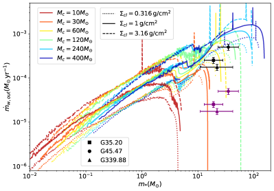
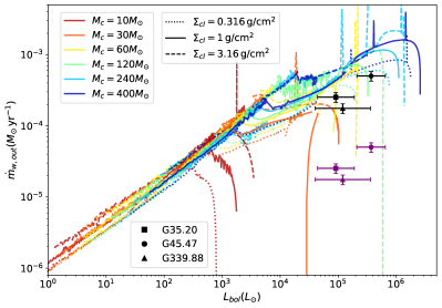
Figure 21: Evolution of mass outflow rate as a function of protostellar mass $m_{*}$ (left) and bolometric luminosity $L_{\rm bol}$ (right) along various protostellar evolutionary sequences. These sequences are characterized by different clump mass surface densities $\Sigma_{\rm cl}$ and initial core masses $M_{c}$ (Zhang & Tan, 2018). The square, circle, and triangle symbols represent the data points for G35.20, G45.47, and G339.88, respectively. The purple symbols represent the raw values of the mass outflow rates, while the black symbols represent the corrected values after applying a correction factor of 10 to the mass outflow rates.

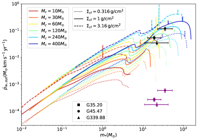
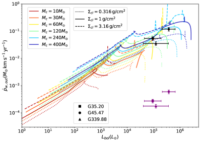
Figure 22: Evolution of momentum outflow rate as a function of protostellar mass $m_{*}$ (left) and bolometric luminosity $L_{\rm bol}$ (right) along various protostellar evolutionary sequences. These sequences are characterized by different clump mass surface densities $\Sigma_{\rm cl}$ and initial core masses $M_{c}$ (Zhang & Tan, 2018). The square, circle, and triangle symbols represent the data points for G35.20, G45.47, and G339.88, respectively. The purple symbols represent the raw values of the momentum outflow rates, while the black symbols represent the corrected values after applying a correction factor of 200 to the momentum outflow rates.

In this section, we calculate the mass outflow rate and momentum outflow rate for the three observed outflows. The method used for these calculations follows the approach described in § 3.3. Additionally, we determine the mass-weighted mean LOS velocity and dynamical timescale of these outflows, using the procedure explained in § 3.4. For estimating the typical outflow length, we assume a one-sided lobe of the outflow corresponding to a half-length of approximately 15 arcseconds (Zhang et al., 2019a). The obtained mass outflow rates and momentum outflow rates for the three outflows are summarized in Table 3.

In §4.2, we determined the inclination angle of the three outflows, and all of them are likely to have an inclination angle exceeding 60 degrees. When the inclination angle falls within the range of 60 to 70 degrees, the conversion factor between the true mass outflow rate and the observed mass outflow rate is approximately 10, while the conversion factor between the true momentum outflow rate and the observed momentum outflow rate is around 200. Based on this, we derived the final estimates for the mass outflow rates of G35.20, G45.47, and G339.88 as $2.53\times 10^{-4}M_{\odot}\,{\rm yr}^{-1}$, $5.01\times 10^{-4}M_{\odot}\,{\rm yr}^{-1}$, and $1.76\times 10^{-4}M_{\odot}\,{\rm yr}^{-1}$, respectively. Additionally, our final estimations for the momentum outflow rates of G35.20, G45.47, and G339.88 are $5.43\times 10^{-2}M_{\odot}{\rm km\,s^{-1}\,yr}^{-1}$, $1.19\times 10^{-1}M_{\odot}{\rm km\,s^{-1}\,yr}^{-1}$, and $3.55\times 10^{-2}M_{\odot}{\rm km\,s^{-1}\,yr}^{-1}$, respectively.

We then place the values for the three sources on the protostellar evolutionary tracks obtained from Zhang & Tan (2018). The protostellar mass $m_{*}$ and bolometric luminosity $L_{\rm bol}$ are determined from SED fitting as reported in Fedriani et al. (2023). Figure 21 illustrates the evolution of mass outflow rate as a function of $m_{*}$ and $L_{\rm bol}$ along various protostellar evolutionary sequences. After applying a correction factor of 10 to the observed mass outflow rate, the final mass outflow rate aligns more closely with the theoretical protostellar evolutionary tracks, though some potential underestimation is still apparent. Figure 22 presents the evolution of momentum outflow rate as a function of $m_{*}$ and $L_{\rm bol}$ along various protostellar evolutionary sequences. After correcting the observed momentum outflow rate by a factor of 200, the final momentum outflow rate closely follows the theoretical protostellar evolutionary tracks. Thus these measurements can help to constrain intrinsic protostellar properties, complementing SED fitting methods, which suffer from significant degeneracies (e.g., Fedriani et al., 2023).

5 Conclusions

In this study, we have used radmc-3d and CASA/simalma to perform radiative transfer and generate synthetic molecular line emission images from 3D MHD simulations of a disk wind outflow. The main results are summarized as follows:

1. We have presented synthetic observations of the outflows for multiple transitions of ¹²CO, ¹³CO, and C¹⁸O. Our analysis shows that the observed opening angle of the outflow cavity increases as the protostellar mass increases. Moreover, the high-velocity components of the outflow are located closer to the outflow launching axis than the low-velocity components. As the inclination angle decreases, more of the outflow forward velocity falls along the line-of-sight, and the high-velocity components become more prominent and adopt a larger spatial distribution.

2. Synthetic interferometric observations of ¹²CO(2-1) outflows were simulated using CASA/simalma, and these synthetic ALMA ¹²CO(2-1) spectra were then compared with three observed ALMA ¹²CO(2-1) spectra. The fitting results provide constraints on the protostellar mass-to-initial core mass ratio and the inclination angle of these outflows, which are found to be consistent with estimates obtained through other methods.

3. We quantify the unobservable outflow mass and compare it with the observable mass. While outflow gas with LOS velocities exceeding 50 km s^-1 is negligible compared to that with LOS velocities between 3 and 50 km s^-1, a significant amount of mass, about ten times or more, is overlooked near the rest frame velocity ($v_{\rm LOS}<3$ km s^-1).

4. We analyze the conversion factor between the total 3D momentum and kinetic energy and the 1D LOS momentum and kinetic energy. Although the high-velocity gas ($v_{\rm LOS}>50$ km s^-1) has negligible mass, it significantly contributes to the overall momentum and energy. Consequently, when estimating the total 3D momentum and energy from the LOS momentum with an absolute LOS velocity ranging from 3 to 50 km s^-1, there is a probable underestimation of the total 3D momentum and 3D energy by a factor of 4 and 50, respectively.

5. The estimated outflow masses derived from the raw ¹²CO(2-1), ¹³CO(1-0), and synthetic ALMA ¹²CO(2-1) spectra show a scattering factor of 4, 2, and 8, respectively, when compared to the true values obtained from the simulation.

6. The estimated outflow momentum and energy derived from the raw ¹²CO(2-1), ¹³CO(1-0), and synthetic ALMA ¹²CO(2-1) spectra show a scatter within a factor of 4 when compared to the true values obtained from the simulation.

7. We have quantified the mass outflow rate and momentum outflow rate from the synthetic ALMA ¹²CO(2-1) spectra and compared them with the true values derived from simulations. Generally, a conversion factor of 10 is needed to obtain the true mass outflow rate, and a conversion factor of 200 is required for the true momentum outflow rate from the synthetic ALMA ¹²CO(2-1) spectra. Furthermore, we have examined the variation of these conversion factors as a function of viewing inclination angles.

8. We computed the mass outflow rate and momentum outflow rate for the three sources, G35.20, G45.47, and G339.88. After applying correction factors of 10 and 200 to the observed mass outflow rate and momentum outflow rate, respectively, both rates closely align with the theoretical protostellar evolutionary tracks. Thus these measurements can help to constrain intrinsic protostellar properties, as a complement to SED fitting.

D.X. and J.P.R. acknowledge support from the Virginia Initiative on Cosmic Origins (VICO). J.C.T. acknowledges support from NSF grant AST-2009674 and ERC Advanced Grant MSTAR. JPR is supported in part by NSF grants AST-1910106, AST-1910675, and NASA grant 80NSSC20K0533. The authors acknowledge Research Computing at The University of Virginia for providing computational resources and technical support that have contributed to the results reported within this publication. The authors further acknowledge the use of NASA High-End Computing (HEC) resources through the NASA Advanced Supercomputing (NAS) division at Ames Research Center to support this work.

Appendix A Moment Maps of Synthetic Outflows

In this section, we present a gallery of moment maps of synthetic outflows as shown in Figure 23-25.

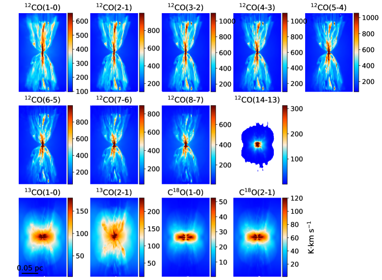
Figure 23: Moment zero maps (integrated intensity) of multiple transitions of ¹²CO, ¹³CO  and C¹⁸O  of the outflow from a 12 $M_{\mathord{\odot}}$ star at an inclination angle of 58^∘.

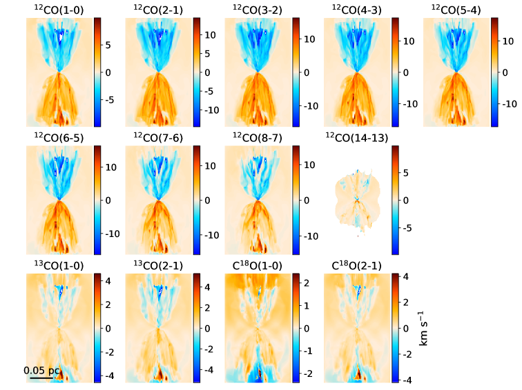
Figure 24: Moment one maps (velocity field) of multiple transitions of ¹²CO, ¹³CO  and C¹⁸O  of the outflow from a 12 $M_{\mathord{\odot}}$ star at an inclination angle of 58^∘.

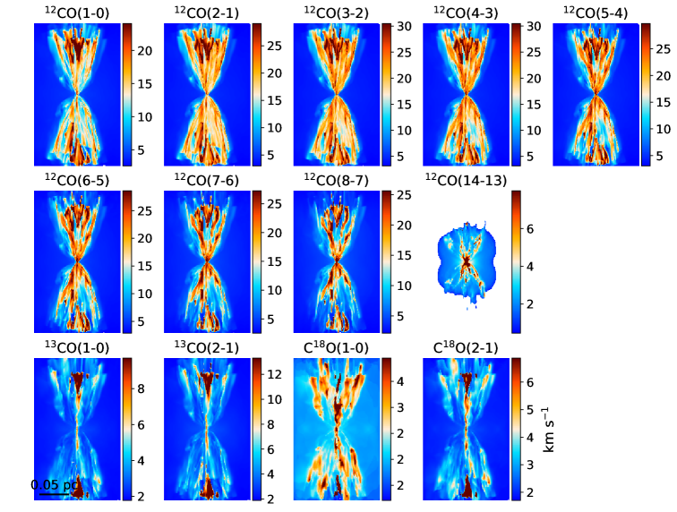
Figure 25: Full width at half maximum (FWHM) maps of multiple transitions of ¹²CO, ¹³CO  and C¹⁸O  of the outflow from a 12 $M_{\mathord{\odot}}$ star at an inclination angle of 58^∘.

Appendix B Estimates of Mass, Momentum, and Energy of Synthetic Outflows using ¹²CO (1-0)

In this section, we report the mass, momentum, and energy estimates of synthetic outflows based on the ¹²CO (1-0) line emission and evaluate their accuracy against the actual values obtained directly from the simulations. The comparison between the ¹²CO (1-0) estimates and the actual values is illustrated in Figure 26.

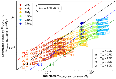
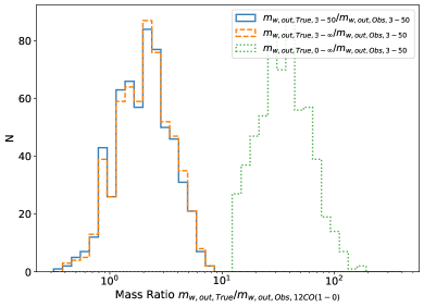
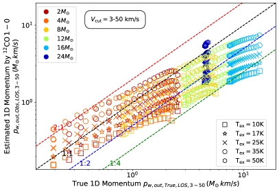
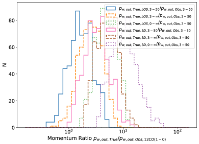
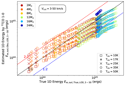
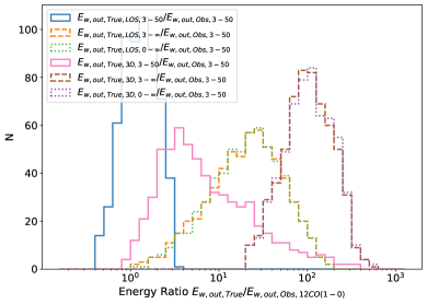
Figure 26: Left column: Comparison of the mass ($1^{st}$ row), momentum ($2^{nd}$ row) and energy ($3^{rd}$ row) estimates obtained for different inclination angles using ¹²CO(1-0) with a LOS velocity cutoff between 3 to 50 km s^-1, and the corresponding true outflow values with the same velocity cutoff. Right column: the ratios between ¹²CO(1-0) calculated mass ($1^{st}$ row), momentum ($2^{nd}$ row) and energy ($3^{rd}$ row) and the true simulation-derived values for different LOS velocity cuts.

References

- Arce & Sargent (2006) Arce, H. G., & Sargent, A. I. 2006, ApJ, 646, 1070, doi: 10.1086/505104
- Bally (2016) Bally, J. 2016, ARA&A, 54, 491, doi: 10.1146/annurev-astro-081915-023341
- Bjerkeli et al. (2016) Bjerkeli, P., van der Wiel, M. H. D., Harsono, D., Ramsey, J. P., & Jørgensen, J. K. 2016, Nature, 540, 406, doi: 10.1038/nature20600
- Blandford & Payne (1982) Blandford, R. D., & Payne, D. G. 1982, MNRAS, 199, 883, doi: 10.1093/mnras/199.4.883
- Bonnell & Bate (2002) Bonnell, I. A., & Bate, M. R. 2002, MNRAS, 336, 659, doi: 10.1046/j.1365-8711.2002.05794.x
- Bonnell & Bate (2006) —. 2006, MNRAS, 370, 488, doi: 10.1111/j.1365-2966.2006.10495.x
- Caratti o Garatti et al. (2015) Caratti o Garatti, A., Stecklum, B., Linz, H., Garcia Lopez, R., & Sanna, A. 2015, A&A, 573, A82, doi: 10.1051/0004-6361/201423992
- de Valon et al. (2020) de Valon, A., Dougados, C., Cabrit, S., et al. 2020, A&A, 634, L12, doi: 10.1051/0004-6361/201936950
- de Valon et al. (2022) —. 2022, A&A, 668, A78, doi: 10.1051/0004-6361/202141316
- Dullemond et al. (2012) Dullemond, C. P., Juhasz, A., Pohl, A., et al. 2012, RADMC-3D: A multi-purpose radiative transfer tool, Astrophysics Source Code Library, record ascl:1202.015. http://ascl.net/1202.015
- Fedriani et al. (2019) Fedriani, R., Caratti o Garatti, A., Purser, S. J. D., et al. 2019, Nature Communications, 10, 3630, doi: 10.1038/s41467-019-11595-x
- Fedriani et al. (2023) Fedriani, R., Tan, J. C., Telkamp, Z., et al. 2023, ApJ, 942, 7, doi: 10.3847/1538-4357/aca4cf
- Ferreira (1997) Ferreira, J. 1997, A&A, 319, 340, doi: 10.48550/arXiv.astro-ph/9607057
- Frank et al. (2014) Frank, A., Ray, T. P., Cabrit, S., et al. 2014, in Protostars and Planets VI, ed. H. Beuther, R. S. Klessen, C. P. Dullemond, & T. Henning, 451–474, doi: 10.2458/azu_uapress_9780816531240-ch020
- Gressel et al. (2015) Gressel, O., Turner, N. J., Nelson, R. P., & McNally, C. P. 2015, ApJ, 801, 84, doi: 10.1088/0004-637X/801/2/84
- Grudić et al. (2022) Grudić, M. Y., Guszejnov, D., Offner, S. S. R., et al. 2022, MNRAS, 512, 216, doi: 10.1093/mnras/stac526
- Hirota et al. (2017) Hirota, T., Machida, M. N., Matsushita, Y., et al. 2017, Nature Astronomy, 1, 0146, doi: 10.1038/s41550-017-0146
- Klassen et al. (2016) Klassen, M., Pudritz, R. E., Kuiper, R., Peters, T., & Banerjee, R. 2016, ApJ, 823, 28, doi: 10.3847/0004-637X/823/1/28
- Lee et al. (2017) Lee, C.-F., Ho, P. T. P., Li, Z.-Y., et al. 2017, Nature Astronomy, 1, 0152, doi: 10.1038/s41550-017-0152
- López-Vázquez et al. (2023) López-Vázquez, J. A., Zapata, L. A., & Lee, C.-F. 2023, arXiv e-prints, arXiv:2301.07877, doi: 10.48550/arXiv.2301.07877
- Lynden-Bell (1996) Lynden-Bell, D. 1996, MNRAS, 279, 389, doi: 10.1093/mnras/279.2.389
- Mattia & Fendt (2020) Mattia, G., & Fendt, C. 2020, ApJ, 900, 59, doi: 10.3847/1538-4357/aba9d7
- Matzner & McKee (1999) Matzner, C. D., & McKee, C. F. 1999, ApJ, 526, L109, doi: 10.1086/312376
- McKee & Tan (2003) McKee, C. F., & Tan, J. C. 2003, ApJ, 585, 850, doi: 10.1086/346149
- Mestel (1968) Mestel, L. 1968, MNRAS, 138, 359, doi: 10.1093/mnras/138.3.359
- Norman (2000) Norman, M. L. 2000, in Revista Mexicana de Astronomia y Astrofisica Conference Series, Vol. 9, Revista Mexicana de Astronomia y Astrofisica Conference Series, ed. S. J. Arthur, N. S. Brickhouse, & J. Franco, 66–71, doi: 10.48550/arXiv.astro-ph/0005109
- Ossenkopf (1997) Ossenkopf, V. 1997, New A, 2, 365, doi: 10.1016/S1384-1076(97)00026-2
- Ouyed et al. (2003) Ouyed, R., Clarke, D. A., & Pudritz, R. E. 2003, ApJ, 582, 292, doi: 10.1086/344507
- Pudritz & Norman (1983) Pudritz, R. E., & Norman, C. A. 1983, ApJ, 274, 677, doi: 10.1086/161481
- Pudritz & Norman (1986) —. 1986, ApJ, 301, 571, doi: 10.1086/163924
- Rosen (2022) Rosen, A. L. 2022, ApJ, 941, 202, doi: 10.3847/1538-4357/ac9f3d
- Sánchez-Monge et al. (2013) Sánchez-Monge, Á., Cesaroni, R., Beltrán, M. T., et al. 2013, A&A, 552, L10, doi: 10.1051/0004-6361/201321134
- Shu et al. (1994) Shu, F., Najita, J., Ostriker, E., et al. 1994, ApJ, 429, 781, doi: 10.1086/174363
- Staff et al. (2015) Staff, J. E., Koning, N., Ouyed, R., Thompson, A., & Pudritz, R. E. 2015, MNRAS, 446, 3975, doi: 10.1093/mnras/stu2392
- Staff et al. (2010) Staff, J. E., Niebergal, B. P., Ouyed, R., Pudritz, R. E., & Cai, K. 2010, ApJ, 722, 1325, doi: 10.1088/0004-637X/722/2/1325
- Staff et al. (2023) Staff, J. E., Tanaka, K. E. I., Ramsey, J. P., Zhang, Y., & Tan, J. C. 2023, ApJ, 947, 40, doi: 10.3847/1538-4357/acbd47
- Staff et al. (2019) Staff, J. E., Tanaka, K. E. I., & Tan, J. C. 2019, ApJ, 882, 123, doi: 10.3847/1538-4357/ab36b3
- Zhang & Tan (2011) Zhang, Y., & Tan, J. C. 2011, ApJ, 733, 55, doi: 10.1088/0004-637X/733/1/55
- Zhang & Tan (2018) —. 2018, ApJ, 853, 18, doi: 10.3847/1538-4357/aaa24a
- Zhang et al. (2014) Zhang, Y., Tan, J. C., & Hosokawa, T. 2014, ApJ, 788, 166, doi: 10.1088/0004-637X/788/2/166
- Zhang et al. (2013) Zhang, Y., Tan, J. C., & McKee, C. F. 2013, ApJ, 766, 86, doi: 10.1088/0004-637X/766/2/86
- Zhang et al. (2018) Zhang, Y., Higuchi, A. E., Sakai, N., et al. 2018, ApJ, 864, 76, doi: 10.3847/1538-4357/aad7ba
- Zhang et al. (2019a) Zhang, Y., Tan, J. C., Sakai, N., et al. 2019a, ApJ, 873, 73, doi: 10.3847/1538-4357/ab0553
- Zhang et al. (2019b) Zhang, Y., Tanaka, K. E. I., Rosero, V., et al. 2019b, ApJ, 886, L4, doi: 10.3847/2041-8213/ab5309
- Zhang et al. (2022) Zhang, Y., Tanaka, K. E. I., Tan, J. C., et al. 2022, ApJ, 936, 68, doi: 10.3847/1538-4357/ac847f